Reconstruction and Simulation of Elastic Objects with Spring-Mass 3D Gaussians

Abstract

Reconstructing and simulating elastic objects from visual observations is crucial for applications in computer vision and robotics. Existing methods, such as 3D Gaussians, provide modeling for 3D appearance and geometry but lack the ability to simulate physical properties or optimize parameters for heterogeneous objects. We propose Spring-Gaus, a novel framework that integrates 3D Gaussians with physics-based simulation for reconstructing and simulating elastic objects from multi-view videos. Our method utilizes a 3D Spring-Mass model, enabling the optimization of physical parameters at the individual point level while decoupling the learning of physics and appearance. This approach achieves great sample efficiency, enhances generalization, and reduces sensitivity to the distribution of simulation particles. We evaluate Spring-Gaus on both synthetic and real-world datasets, demonstrating accurate reconstruction and simulation of elastic objects. This includes future prediction and simulation under varying initial states and environmental parameters. Project page: https://zlicheng/spring_gaus.

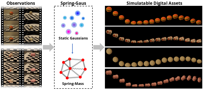
Figure 1: Spring-Gaus identifies the intrinsic physical properties of elastic objects from video observations, learning a physical model over an abstracted spatial representation through explicit spring-mass modeling. The model’s output can be regarded as simulatable digital assets, enabling capabilities such as future prediction and simulation under different initial states and scene parameters.

1 Introduction

Reconstructing and simulating elastic objects from visual observations is a fundamental challenge in computer vision and robotics, with applications in virtual reality, augmented reality, and robotic manipulation. Accurately modeling object elasticity is crucial for creating immersive experiences and enabling embodied agents to understand and interact with the challenging yet common elastic objects encountered in our daily lives.

Existing methods for dynamic scene reconstruction, such as 3D Gaussians and their dynamic extensions [14, 26, 44, 49], have made significant progress in capturing the appearance and geometry of objects from multi-view images. However, these methods often lack the ability to capture the physical properties of the reconstructed objects, thus limiting their ability to simulate object motion and their application in interactive environments. While some approaches, such as PhysGaussian [46] and PAC-NeRF [18], attempt to integrate physics into the reconstruction process, they face challenges in optimizing physical parameters for individual object elements, especially in the case of heterogeneous objects. Moreover, the implicit representation used in PAC-NeRF can lead to a degradation of appearance over time.

In this paper, we propose Spring-Gaus, a novel framework that addresses these limitations by integrating 3D Gaussians with physics-based simulation for reconstructing and simulating elastic objects from multi-view videos (Fig. 1). Our method utilizes a 3D Spring-Mass Model for simulating object deformation, which enables optimization of physical parameters at the individual point level. By decoupling physics learning from appearance learning, Spring-Gaus preserves the geometric shapes and appearance features of the reconstructed objects during training, even in the presence of image errors. The abstract and physics-integrated nature of our simulation approach grants Spring-Gaus significant sample efficiency, enhanced generalization capabilities, and reduced sensitivity to the number and spatial distribution of simulation particles.

We evaluate the effectiveness of Spring-Gaus on both synthetic and real-world datasets, demonstrating its ability to accurately reconstruct and simulate elastic objects. Our method can predict future deformations and perform simulations under varying initial states and environmental parameters, showcasing its potential for applications in predictive visual perception and immersive experiences. In summary, the main contributions of this work are threefold:

• We propose Spring-Gaus, a novel framework that integrates 3D Gaussians with physics-based simulation for the reconstruction and simulation of elastic objects from multi-view videos.

• We incorporate a 3D Spring-Mass Model for simulating object deformation, enabling the optimization of physical parameters at the individual point level while decoupling the learning of physics and appearance.

• We demonstrate the effectiveness of Spring-Gaus on both synthetic and real-world datasets, showcasing accurate reconstruction and simulation of elastic objects. This includes capabilities for future prediction and simulation under varying initial configurations.

2 Related Work

3D Neural Scene Representations:  Scene Representation Networks (SRNs) [38] and DeepSDF [29] represent significant advancements in scene representation, treating scenes as continuous functions that map world coordinates to a feature representation of local scene properties. Over the past few years, NeRF [28] and its successors [50, 2, 1, 25, 47] have demonstrated the efficacy of neural networks in capturing continuous 3D scenes through implicit representation. DirectVoxGO [40] accelerates NeRF’s approach by substituting the MLP with a voxel grid. Furthermore, 3D Gaussian Splatting [14] has emerged as a method for real-time differentiable rendering, representing scenes with 3D Gaussians. Extending this approach, DreamGaussian [41] applies 3D Gaussian Splatting for 3D content generation. Additionally, PhysGaussian [46] integrates physical information into 3D Gaussians using a customized Material Point Method. Unlike these approaches, our method focuses on identifying 3D digital assets from multi-view videos through a 3D Gaussian representation, offering a novel perspective on digital asset acquisition.

Dynamic Reconstruction:  The modeling of dynamic scenes has seen significant progress with the adoption of NeRF [32, 18, 22, 42, 30, 10, 20, 8, 23, 51, 43, 31] and 3D Gaussian [26, 49, 44, 24, 52, 12, 16, 48] representations. D-NeRF [32] introduces an extension to NeRF, capable of modeling dynamic scenes from monocular views by optimizing an underlying deformable volumetric function. Furthermore, Dynamic 3D Gaussians [26] focus on optimizing the motion of Gaussian kernels for each frame, presenting an efficient method to capture scene dynamics. Deformable 3D Gaussians [49] propose a novel approach by learning Gaussian distributions in a canonical space, complemented with a deformation field for modeling monocular dynamic scenes. Meanwhile, 4D Gaussian Splatting [44] introduces a hybrid model combining 3D Gaussians with 4D neural voxels. PAC-NeRF [18] delves into the integration of Lagrangian particle simulation with Eulerian scene representation, exploring a new aspect in scene dynamics. In this paper, we introduce a simulation pipeline that operates directly on abstracted spatial representations based on 3D Gaussian kernels from a Lagrangian perspective, furthering the capabilities in dynamic physical scene reconstruction.

Physics-Informed Learning:  Physics-Informed Learning has emerged as a prominent research direction since the introduction of Physics-Informed Neural Networks (PINNs) [33]. Li et al. [21] and Sanchez-Gonzalez et al. [34] introduced Graph Network-based simulators within a machine learning framework. INSR-PDE [3] tackles time-dependent partial differential equations (PDEs) using implicit neural spatial representations. NCLaw [27] focuses on learning neural constitutive laws for PDE dynamics. DiffPD [9] presents a differentiable soft-body simulator. Li et al. [19] have made strides in learning preconditioners for conjugate gradient PDE solvers. Chu et al. [4] modeled smoke in neural density and velocity fields. Neural Flow Maps [7] integrate fluid simulation with neural implicit representations. Deng et al. [6] introduced a novel differentiable vortex particle method for fluid dynamics inference. DANOs [17] stores objects’ geometry in a neural density field. PAC-NeRF [18] learns physical parameters used in MPM simulations. Our work extends the application of physics-informed learning to 3D Gaussian kernels, enabling the reconstruction and simulation of dynamic scenes with physical properties.

3 Preliminary

This section introduces 3D Gaussian Splatting [14], the foundational method underlying our approach. Gaussian Splatting employs a set of 3D Gaussian kernels to represent a scene. These kernels are characterized by a full 3D covariance matrix $\Sigma$, defined in world space and centered at point $\bm{\mu}$:

$$G(\bm{x})=e^{-\frac{1}{2}(\bm{x})^{T}\Sigma^{-1}(\bm{x})},$$ (1)

where $\bm{\mu}$ is the mean of the Gaussian distribution, and $\bm{x}$ is the independent variable of the Gaussian distribution. The covariance matrix $\Sigma$ can be decomposed into a rotation matrix $R$ and a scaling matrix $S$, such that $\Sigma=RSS^{T}R^{T}$.

The Splatting process, designed to render Gaussian kernels into a 2D image, involves two main steps: (1) projecting the Gaussian kernels into camera space, and (2) rendering the projected kernels into image space. The projection process is defined as:

$$\Sigma^{\prime}=JW\Sigma W^{T}J^{T},$$ (2)

where $\Sigma^{\prime}$ represents the covariance matrix in camera coordinates, $W$ is the transformation matrix, and $J$ denotes the Jacobian of the affine approximation of the projective transformation. The rendered color $C$ of each pixel is computed as:

$$C=\sum_{i\in N}T_{i}\alpha_{i}\bm{c_{i}},$$ (3)

where $T_{i}$ represents the transmittance, defined as $\Pi_{j=1}^{i-1}\alpha_{j}$. The term $\alpha_{i}$ denotes the alpha value for each Gaussian, which is calculated using the expression $1-e^{-\sigma_{i}\delta_{i}}$, where $\sigma_{i}$ is the opacity factor. Additionally, $\bm{c_{i}}$ refers to the color of the Gaussian along the ray within the interval $\delta_{i}$.

The learnable parameters for each Gaussian kernel include a point center $\bm{\mu}$, a 3D scaling vector $\bm{s}$, a quaternion $\bm{q}$, a color $\bm{c}$, an opacity factor $\sigma$, and a set of spherical harmonics (SH) coefficients. These SH coefficients are employed to represent the view-dependent component of the radiance field.

4 Approach

We propose Spring-Gaus that integrates a 3D Spring-Mass model with 3D Gaussians for elastic object reconstruction and simulation. We show an overview in Fig. 2. In the following, we elaborate each component of our approach.

4.1 Static Reconstruction

Given a set of posed videos captured by $n$ cameras over $f$ frames, denoted as $\{{I_{i,j}}\}_{i=0,j=0}^{n,f}$, we utilize the first frame from each sequence, $\{I_{i,0}\}_{i=0}^{n}$, to reconstruct the initial static scene. In our formulation, we assume all Gaussian kernels are isotropic, simplifying our model by omitting the quaternion $\bm{q}$ and spherical harmonics (SH) coefficients. Consequently, we transform the scaling vector $\bm{s}\in\mathbb{R}^{3}$ into a scalar $s\in\mathbb{R}$. For each kernel, the learnable parameters include a point center $\bm{\mu}$, a scaling scalar $s$, a color vector $\bm{c}$, and an opacity value $\sigma$.

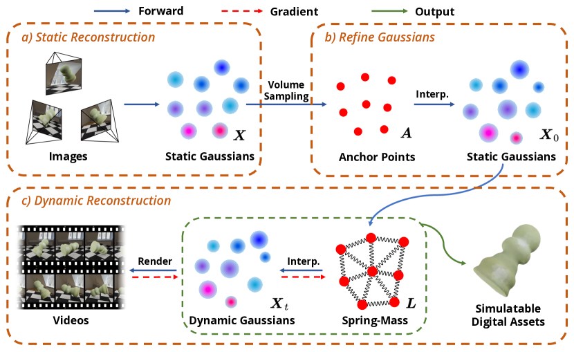
Figure 2: Pipeline of Spring-Gaus: (a) Static Scene Reconstruction: Initially, we extract static 3D Gaussians from the first frame of the video. (b) Refining 3D Gaussians: During the dynamic process, the center positions of Gaussian kernels, derived from anchor points, slightly deviate from static reconstruction results. To correct this, we adjust the kernels’ color, scale, and opacity values, refining the 3D Gaussians for accurate rendering. (c) Dynamic Reconstruction: We employ a specialized Spring-Mass model to simulate anchor points and concurrently update the positions of Gaussian kernels. Upon completion of training, we obtain a simulatable digital object that accurately reflects dynamic behaviors.

4.2 Dynamic Reconstruction

Building on the static scene reconstruction, we obtain a set of Gaussian kernels $\{G_{i}\}_{i=1}^{N}$, complete with corresponding point centers $\bm{X}=\{\bm{\mu}_{i}\}_{i=1}^{N}$, scaling scalars $\{s_{i}\}_{i=1}^{N}$, color vectors $\{\bm{c}_{i}\}_{i=1}^{N}$, and opacity values $\{\sigma_{i}\}_{i=1}^{N}$.

To manage complexity, we introduce volume sampling to generate a set of anchor points $\bm{A}=\{\bm{x}_{i}\}_{i=1}^{N_{A}}$, defined by:

$$\bm{A}=\{\bm{x}_{i}\}_{i=1}^{N_{A}}=\mathcal{V}(\bm{X}),$$ (4)

where $N_{A}$ represents the number of anchors, and $\mathcal{V}$ symbolizes the sampling function. We adopt a Spring-Mass model which can simulate the motion of anchor points $\bm{A}$, assuming each anchor has a mass $m_{i}$ and an initial velocity $\bm{v}_{i}$. Each anchor $\bm{x}_{i}$ connects to its $n_{k}$ nearest neighbors $\bm{N}_{i}=\{\bm{x}_{i,j}\}_{j=1}^{n_{k}}$ through springs $\bm{L}$, defined as:

$$\bm{L}=\{l_{i,j}\}_{i=1,j=1}^{N_{A},n_{k}}=\mathrm{knn}(\bm{A},\bm{A},n_{k}),$$ (5)

where $l_{i,j}$ signifies the spring’s length between $\bm{x}_{i}$ and $\bm{x}_{i,j}$, and $\mathrm{knn}$ denotes the k-nearest neighbors function. Each spring is characterized by a stiffness $k_{i,j}$ and a damping factor $\zeta_{i,j}$.

To adjust the Gaussian kernels’ positions, we initially measure the distance between each kernel center and its $n_{b}$ nearest anchors at the dynamic simulation’s onset:

$$\{d_{i,j}\}_{i=1,j=1}^{N,n_{b}}=\mathrm{knn}(\mathcal{X},\mathcal{A},n_{b}).$$ (6)

For each timestep $t$, the forces $\bm{F}_{i}^{t}$ acting on each anchor point $\bm{x}_{i}^{t}$ are calculated as follows:

$$\bm{F}_{i}^{t}={\bm{F_{k}}}_{i}^{t}+{\bm{F_{\zeta}}}_{i}^{t}+m_{i}\bm{g},$$ (7)

where ${\bm{F_{k}}}_{i}^{t}$, ${\bm{F_{\zeta}}}_{i}^{t}$ and $\bm{g}$ represent the spring force, the damping force and gravitational acceleration, respectively.

To address the significant impact that the value of $n_{k}$ has on the simulation—where a smaller value of $n_{k}$ leads to a noticeably softer behavior of the point cloud—we introduce a mitigation strategy by applying a soft vector $\eta=[\eta_{0},\eta_{1},...,\eta_{n_{k}}]$. This vector controled by a learnable parameter $\kappa$ is used to modulate the number of connected springs, thereby adjusting the system’s response to different object, while we do not expect the chosen of $n_{k}$ will limit the generalization ability of the model. The soft vector $\eta$ is calculated as:

$$\eta_{i}=\left\{\begin{aligned} &1&&i\leq n_{c},\\ &\mathrm{clamp}(2-\exp(\mathrm{softplus}(\kappa))^{i-n_{c}},0,1)&&n_{c}<i\leq n_{k}.\end{aligned}\right.$$ (8)

Then, for each spring $\bm{L}_{i,j}$, the spring force ${\bm{F_{k}}}_{i,j}^{t}$ and damping force ${\bm{F_{\zeta}}}_{i,j}^{t}$ are determined by:

$${\bm{F_{k}}}_{i,j}^{t}=-\eta_{j}\cdot k_{i,j}\left(\left\|\bm{x}_{i}^{t}-\bm{x}_{i,j}^{t}\right\|-l_{i,j}\right)\frac{\bm{x}_{i}^{t}-\bm{x}_{i,j}^{t}}{\left\|\bm{x}_{i}^{t}-\bm{x}_{i,j}^{t}\right\|}\cdot{\Big{|}\left\|\bm{x}_{i}^{t}-\bm{x}_{i,j}^{t}\right\|-l_{i,j}\Big{|}}^{p_{k}},$$ (9)

$${\bm{F_{\zeta}}}_{i,j}^{t}=\left(-\zeta_{i,j}\left(\bm{v}_{i}^{t}-\bm{v}_{i,j}^{t}\right)\frac{\bm{x}_{i}^{t}-\bm{x}_{i,j}^{t}}{\left\|\bm{x}_{i}^{t}-\bm{x}_{i,j}^{t}\right\|}\right)\cdot\frac{\bm{x}_{i}^{t}-\bm{x}_{i,j}^{t}}{\left\|\bm{x}_{i}^{t}-\bm{x}_{i,j}^{t}\right\|},$$ (10)

where, when $p_{k}$ is set to $0$, Eq. 9 becomes the Hooke’s law, and for positive values of $p_{k}$, the spring force becomes a nonlinear function of the spring’s length. The cumulative forces acting on each anchor point $\bm{x}_{i}^{t}$ are expressed as:

$$\bm{F}_{i}^{t}=\sum_{j=1}^{n_{k}}{\bm{F_{k}}}_{i,j}^{t}+\sum_{j=1}^{n_{k}}{\bm{F_{\zeta}}}_{i,j}^{t}+m_{i}\bm{g}.$$ (11)

Anchor points $\bm{A}$’s positions and velocities are updated using semi-implicit Euler integration:

$$\bm{v}_{i}^{t+1}=\bm{v}_{i}^{t}+\frac{\bm{F}_{i}^{t}}{m_{i}}\Delta t,$$ (12)

$$\bm{x}_{i}^{t+1}=\bm{x}_{i}^{t}+\bm{v}_{i}^{t+1}\Delta t,$$ (13)

and a boundary condition $\mathcal{BC}$ is applied to anchor points $\bm{A}$ to ensure physical plausibility:

$$\bm{x}_{i}^{t+1},\bm{v}_{i}^{t+1}=\mathcal{BC}(\bm{x}_{i}^{t+1},\bm{v}_{i}^{t+1}).$$ (14)

The position of each Gaussian kernel $\bm{\mu}_{i}$ is updated through Inverse Distance Weighting (IDW) interpolation to reflect the dynamic changes accurately:

$$\bm{\mu}_{i}^{t+1}=\frac{\sum_{j=1}^{n_{b}}{\bm{x}_{i,j}^{t+1}}\cdot(1/{(d_{i,j}^{t+1})}^{p_{b}})}{\sum_{j=1}^{n_{b}}(1/{(d_{i,j}^{t+1})}^{p_{b}})},$$ (15)

where $p_{b}$ is a positive real number that determines the diminishing influence of anchor points with distance. To render the image $\hat{I}$ at a specific camera and frame, we use the updated positions of the Gaussian kernels following the rendering equation Eq. 3.

4.3 Optimization

Optimizing all unknown parameters simultaneously in a highly abstract and complex model like ours is inadvisable, as it often leads to suboptimal solutions. Furthermore, the intricacy of our model makes optimization challenging. To address this, we propose a strategy to streamline the model by reducing the number of learnable parameters without altering the underlying calculation process.

In our simplified approach, we standardize the mass of every anchor to a constant value $m_{0}$, and control all damping factors using a singular parameter $\zeta_{0}$. These two parameters are fixed, eliminating their variability from the optimization process. Furthermore, we introduce a unified parameter $k_{i}$ for each anchor $\bm{x}_{i}$ to control the spring stiffness of the springs connected to it, simplifying the model without compromising its functional integrity. The spring stiffness $k_{i,j}$ and damping factor $\zeta_{i,j}$ are thus calculated as follows:

$$k_{i,j}=k_{i}/l_{i,j},$$ (16)

$$\zeta_{i,j}=\zeta_{0}/l_{i,j}.$$ (17)

Summarized, the learnable parameters in our model now include:

• $\bm{v}_{0}$: the initial velocity vector, providing a baseline movement pattern for the simulation;

• $\{{k_{i}}\}_{i=1}^{N_{A}}$: the individual stiffness parameters for each anchor, allowing for localized adjustments to spring stiffness;

• $\kappa$: a parameter governing the modulation of the soft vector, facilitating fine-tuned control over the spring dynamics;

• $\Theta(\mathcal{BC(\cdot)})$: parameters defining the boundary conditions, such as the friction coefficient, which influence the simulation’s physical realism.

By strategically reducing the number of learnable parameters, our model maintains computational efficiency and ease of optimization, while still capturing the essential dynamics of the system under study.

Same with 3D Gaussian Splatting [14], we define our loss function as a weighted combination of the $\mathcal{L}_{1}$ norm and the Structural Similarity Index Measure (D-SSIM) $\mathcal{L}_{\mathit{d-ssim}}$, applied between the input images $I$ and the rendered images $\hat{I}$. This is formally expressed as:

$$\mathcal{L}=(1-\lambda_{\mathit{d-ssim}})\mathcal{L}_{1}+\lambda_{\mathit{d-ssim}}\mathcal{L}_{d-ssim},$$ (18)

where $\lambda_{\mathit{d-ssim}}$ is a weighting coefficient that balances the contribution of the $\mathcal{L}_{1}$ norm and the D-SSIM term to the overall loss. Inspired by PAC-NeRF [18], we first independently optimize the initial velocity vector $\bm{v}_{0}$, utilizing only the few frames captured before the object interacts with the environment.

In terms of the Gaussian kernels’ parameters, we optimize all of them during static scene reconstruction while maintaining a constant scaling scalar $s_{0}$ for all kernels. We have found that uniform scaling across all kernels in static scene reconstruction results in a more evenly distributed point cloud and anchor points. This consistency markedly improves the dynamic model’s simulation capabilities by enhancing spatial distribution. During dynamic simulation, the points center $\bm{\mu}$ is computed as outlined in Eq. 15, which exhibits slight deviations from the static reconstruction results. Therefore, we refine the parameters of the Gaussian kernels—scaling scalar $s$, color vector $\bm{c}$, and opacity value $\sigma$, excluding points center $\bm{\mu}$—before dynamic simulation at the first frame. This refinement ensures the Gaussian kernels adhere to the IDW interpolation results. It is important to note that we DO NOT preserve the scaling scalar as constant $s_{0}$ during this refinement phase. Instead, we assign a unique scaling scalar $s_{i}$ to each Gaussian kernel, given that the anchor points are already established.

5 Experiment

5.1 Datasets

Synthetic Data.  We evaluate Spring-Gaus using a synthetic dataset. We first collected lots of 3D models, including point clouds and meshes, to use as initial point clouds for our simulations. Some of the them are sourced from PAC-NeRF [18] and OmniObject3D [45]. We employ the Material Point Method (MPM) [39, 11] to simulate the behavior of elastic objects derived from point clouds. Our dataset features elastic objects that exhibit a range of softness levels and diverse geometric forms. Multi-view RGB videos are generated using Blender [5], with each sequence comprising 10 viewpoints and 30 frames at a resolution of 512$\times$512. The initial 20 frames are utilized for dynamic reconstruction, while the subsequent 10 frames are dedicated to evaluating future prediction performance.

Real-World Data.  In addition to synthetic datasets, we further assess Spring-Gaus using a few of real-world samples. Our collection process distinguishes between static scenes and dynamic multi-view videos. For static scenes, we position each object on a table and capture 50-70 images from various viewpoints within the upper hemisphere surrounding the object. To obtain camera poses for static scenes, we utilize the off-the-shelf Structure-from-Motion toolkit COLMAP [35, 36]. The dynamic aspect of our dataset is represented through multi-view RGB videos, recorded from three distinct viewpoints using the SONY ILCE-7RM4A camera, at a resolution of 1920$\times$1080. The camera parameters for dynamic scenes are computed from the calibration chessboard. Segment-Anything [15] is used to obatin masks for real world samples.

5.2 Implementation Details

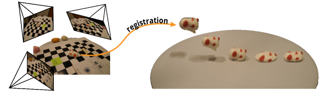
Figure 3: Registration from static scene to dynamic scene for real-world sample.

We train our model on a single NVIDIA RTX 3090 GPU. For static scene reconstruction, we follow to the configuration prescribed by 3D Gaussian Splatting [14], which requires approximately 10 minutes for synthetic data. We train our dynamic model for 300 iterations, taking around 1 hour for synthetic data. We employ 2048 anchor points for our Spring-Mass Model, with each anchor linked to $n_{k}=256$ neighbors through springs. We roughly set $n_{b}=16$ and $n_{c}=16$. For each sequence, we assume mass $m_{0}=1$ and damping factor $\zeta_{0}=0.1$. The weighting coefficient for the D-SSIM term $\lambda_{\mathit{d-ssim}}$ is configured to $0.2$ for static reconstruction and $0.05$ for dynamic reconstruction. In our experiments, we use a nonlinear spring force, setting $p_{k}=0.5$, and for Inverse Distance Weighting (IDW) interpolation, we arbitrarily choose $p_{b}=0.5$.

For real-world samples, we collect static and dynamic scenes separately because three viewpoints are insufficient for effective 3D Gaussian Splatting [14]. This results in the Gaussian kernels for static and dynamic scenes being in different coordinate systems. Therefore, for real samples, we employ a registration network before dynamic reconstruction to align the Gaussian kernels from static scene coordinates to dynamic scene coordinates, as shown in Fig. 3. Specifically, we optimize an additional scale factor $s_{r}$, a translation vector $\bm{t_{r}}$, and a rotation vector $\bm{r_{r}}$. We represent 3D rotations using a continuous 6D vector $\bm{r_{r}}\in\mathbb{R}^{6}$, which has been shown to be more conducive for learning [53].

However, slight deformations of objects and variations in lighting conditions and exposure times during data capture are inevitable. These variations can result in color discrepancies that significantly affect the efficiency of image-based optimization strategies. To mitigate these effects, we refine our approach by computing the loss function between mask images, incorporating both mask center loss and perceptual loss into our model. Consequently, the revised loss function for real samples is expressed as:

$$\mathcal{L}=(1-\lambda_{\mathit{d-ssim}})\mathcal{L}_{1}+\lambda_{\mathit{d-ssim}}\mathcal{L}_{d-ssim}+\lambda_{\mathit{center}}\mathcal{L}_{center}+\lambda_{\mathit{percep}}\mathcal{L}_{percep},$$ (19)

where $\lambda_{\mathit{d-ssim}}=0.8$, $\lambda_{\mathit{center}}=1.0$, and $\lambda_{\mathit{percep}}=0.1$ are the weighting coefficients. Here, $\mathcal{L}_{percep}$ quantifies the discrepancy between the center coordinates of the rendered and ground truth images, while $\mathcal{L}_{percep}$ represents the perceptual loss [13], which is based on the VGG16 architecture [37].

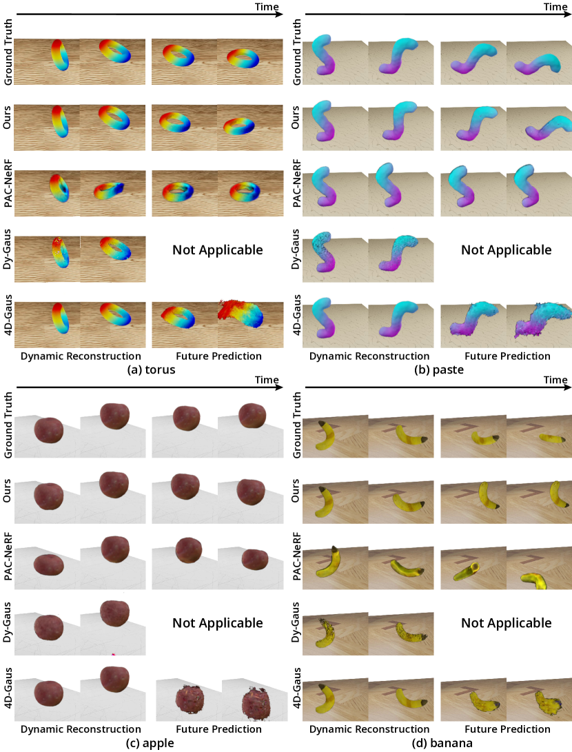
Figure 4: Qualitative results on MPM simulation datas. Compared with PAC-NeRF [18], Dynamic 3D Gaussians [26] and 4D Gaussian Splatting [44].

5.3 Qualitative and Quantitative Results

We assess the performance of Spring-Gaus using both synthetic and real-world datasets. Initially, we validate the effectiveness of our method on synthetic datasets, utilizing the first 20 frames as our observation set for training dynamic modeling capabilities. For evaluating simulatability, we employ the subsequent 10 frames, comparing the ground truth with our model’s predictions of future frames. Additionally, we benchmark Spring-Gaus against key related works in dynamic scene modeling and physics-informed learning methods, including PAC-NeRF [18], Dynamic 3D Gaussians [26], and 4D Gaussian Splatting [44].

		torus	cross	cream	apple	paste	chess	banana	Mean
CD$\downarrow$	Spring-Gaus (ours)	2.38	1.57	2.22	1.87	7.03	2.59	18.48	5.16
	PAC-NeRF [18]	2.47	3.87	2.21	4.69	37.70	8.20	66.43	17.94
EMD$\downarrow$	Spring-Gaus (ours)	0.087	0.051	0.094	0.076	0.126	0.095	0.135	0.095
	PAC-NeRF [18]	0.055	0.111	0.083	0.108	0.192	0.155	0.234	0.134
PSNR$\uparrow$	Spring-Gaus (ours)	16.83	16.93	15.42	21.55	14.71	16.08	17.89	17.06
	PAC-NeRF [18]	17.46	14.15	15.37	19.94	12.32	15.08	16.04	15.77
SSIM$\uparrow$	Spring-Gaus (ours)	0.919	0.940	0.862	0.902	0.872	0.881	0.904	0.897
	PAC-NeRF [18]	0.913	0.906	0.858	0.878	0.819	0.848	0.866	0.870

Table 1: Quantitative results of short-term future prediction on MPM simulation data.

		torus	cross	cream	apple	paste	chess	banana	Mean
CD$\downarrow$	Spring-Gaus (ours)	0.17	0.48	0.36	0.38	0.19	1.80	2.60	0.85
	PAC-NeRF [18]	4.92	1.10	0.77	1.11	3.14	0.96	2.77	2.11
	Dy-Gaus [26]	579	773	479	727	2849	764	2963	1305
	4D-Gaus [44]	11.12	1.77	2.87	2.23	1.95	3.97	7.13	4.43
EMD$\downarrow$	Spring-Gaus (ours)	0.040	0.037	0.031	0.033	0.022	0.063	0.052	0.040
	PAC-NeRF [18]	0.056	0.052	0.041	0.045	0.054	0.052	0.062	0.052
	Dy-Gaus [26]	0.857	0.955	0.783	0.903	1.739	0.985	1.591	1.116
	4D-Gaus [44]	0.130	0.078	0.089	0.088	0.070	0.097	0.112	0.095

Table 2: Quantitative results of dynamic reconstruction on MPM simulation data.

The qualitative results are presented in Fig. 4. We also report quantitative results by computing the Chamfer Distance (CD) and Earth Mover’s Distance(EMD). In all tables, the Chamfer Distance is measured based on squared distance, with units expressed as $1\times 10^{3}mm^{2}$. The quantitative analysis of dynamic modeling, shown in Tab. 2, reveals that Spring-Gaus can accurately learn motions from MPM simulated data.

In Tab. 1, we showcase our method’s capability in predicting future frames. Our method outperforms PAC-NeRF across CD, EMD, Peak Signal-to-Noise Ratio (PSNR), and Structural Similarity Index (SSIM) metrics. Although 4D-Gaus was not specifically designed for future prediction, we tested this approach by inputting a future timestamp into the neural network, which yielded suboptimal results shown in Fig. 4.

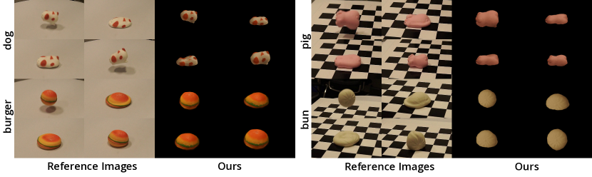
Figure 5: Results on real world samples.

We also evaluate Spring-Gaus on real world samples. It is difficult for both NeRF [28] and 3D Gaussian Splatting [14] to reconstruct the correct geometric information under extremely sparse camera views. However, thanks to 3D Gaussians’ explicit representation, we could reconstruct static scene and dynamic scene in a different coordinate system and then align them using a registration network mentioned in Sec. 5.2, which is hard to do under a implicit representation. We show the registration process in Fig. 3. Results can be found in Fig. 5 and Fig. 1.

5.4 Simulatable Digital Assets

In addition to future prediction. We also demonstrate the capability of our method to simulate digital assets. In Fig. 6, we edit the boundary conditions. In Fig. 7, we edit initialization conditions and environment conditions. Please refer to our supplementary materials for more results.

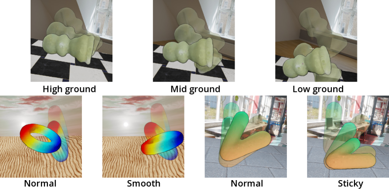
Figure 6: We edit boundary conditions in these demos. Changing grounds’ position and use smooth or sticky ground.

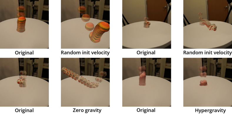
Figure 7: We edit initial velocities, and edit gravity conditions in these demos.

	dynamic reconstruction			future prediction
	CD$\downarrow$	PSNR$\uparrow$	SSIM$\uparrow$	CD$\downarrow$	PSNR$\uparrow$	SSIM$\uparrow$
Spring-Gaus (ours)	0.18	27.08	0.967	2.04	17.63	0.927
Spring-Gaus w/o soft vector $\eta$	0.56	25.36	0.959	13.28	13.91	0.881
Spring-Gaus, single $k$	3.22	23.02	0.940	6.56	14.45	0.892
PAC-NeRF [18]	8.66	19.87	0.916	5.70	15.65	0.894

Table 3: Ablation study. We demonstrate the importance of optimizing parameters for each anchor point individually as well as using a soft vector $\eta$.

5.5 Ablation Study

Figure 8: Ablation study of the effectiveness of optimizing physical parameters for each particle rather than optimizing a single global parameter, on a heterogeneity object.

In our approach, we employ a soft vector $\eta$ to dynamically regulate both the quantity and intensity of springs linked to the anchor points. This strategy is illustrated in Tab. 3, showcasing its effectiveness. Our method’s capability to simulate using very sparse anchors allows for the individual optimization of physical parameters for each anchor point. This contrasts with PAC-NeRF, which utilizes tens of thousands of particles, rendering the optimization of physical parameters for each particle infeasible. Consequently, PAC-NeRF faces limitations in accurately modeling objects composed of inhomogeneous materials. In contrast, our methodology is adept at handling such complexities. As depicted in Fig. 8 and Tab. 3, we present the outcomes on a heterogeneous object that is segmented into various sections, each with distinct physical properties, thereby demonstrating our model’s superior adaptability in capturing the nuanced dynamics of objects with variable material composition.

6 Limiation

In this section, we address the limitations of our approach and outline avenues for future research. Currently, Spring-Gaus is constrained to modeling elastic objects due to the static nature of spring lengths in our formulation; these lengths are constants established at the onset of dynamic simulation. Future work should aim to incorporate plastic deformation into the framework. This would involve developing a method to dynamically adjust the original lengths of the springs during the simulation, allowing for the accurate modeling of materials that exhibit both elastic and plastic behavior.

7 Conclusion

In this paper, we introduce Spring-Gaus, a novel framework designed to acquire simulatable digital assets of elastic objects from video observations. By merging a special 3D Spring-Mass Model with Gaussian kernels, we have modeled dynamic scenes and simulated them within a differentiable pipeline. A key feature of our approach is the distinct separation between the learning processes for appearance and physics, thereby circumventing potential issues with optimization interference. The abstract modeling approach of Spring-Gaus, coupled with its modest requirements on particle distribution and count, endows it with a good capacity for dynamic modeling. We evaluate Spring-Gaus on both synthetic and real-world datasets, demonstrating its capability to reconstruct spatial geometry, temporal dynamics, and appearance while preserving simulatability. Moreover, Spring-Gaus’s proficiency in predicting short-term future dynamics and modifying environmental variables showcases its advanced capabilities in dynamic modeling and physical property identification from observational data.

References

- [1] Barron, J.T., Mildenhall, B., Tancik, M., Hedman, P., Martin-Brualla, R., Srinivasan, P.P.: Mip-NeRF: A multiscale representation for anti-aliasing neural radiance fields. In: CVPR (2021)
- [2] Chen, A., Xu, Z., Zhao, F., Zhang, X., Xiang, F., Yu, J., Su, H.: Mvsnerf: Fast generalizable radiance field reconstruction from multi-view stereo. In: ICCV (2021)
- [3] Chen, H., Wu, R., Grinspun, E., Zheng, C., Chen, P.Y.: Implicit neural spatial representations for time-dependent pdes. In: ICML (2023)
- [4] Chu, M., Liu, L., Zheng, Q., Franz, E., Seidel, H.P., Theobalt, C., Zayer, R.: Physics informed neural fields for smoke reconstruction with sparse data. ACM TOG 41(4) (jul 2022). https://doi.org/10.1145/3528223.3530169
- [5] Community, B.O.: Blender - a 3D modelling and rendering package. Blender Foundation, Stichting Blender Foundation, Amsterdam (2018), http://www.blender.org
- [6] Deng, Y., Yu, H.X., Wu, J., Zhu, B.: Learning vortex dynamics for fluid inference and prediction. In: ICLR (2023)
- [7] Deng, Y., Yu, H.X., Zhang, D., Wu, J., Zhu, B.: Fluid simulation on neural flow maps. ACM TOG 42(6) (2023)
- [8] Driess, D., Huang, Z., Li, Y., Tedrake, R., Toussaint, M.: Learning multi-object dynamics with compositional neural radiance fields. In: Conference on Robot Learning. pp. 1755–1768. PMLR (2023)
- [9] Du, T., Wu, K., Ma, P., Wah, S., Spielberg, A., Rus, D., Matusik, W.: Diffpd: Differentiable projective dynamics. ACM TOG 41(2) (nov 2021). https://doi.org/10.1145/3490168
- [10] Guan, S., Deng, H., Wang, Y., Yang, X.: Neurofluid: Fluid dynamics grounding with particle-driven neural radiance fields. In: ICML (2022)
- [11] Hu, Y., Fang, Y., Ge, Z., Qu, Z., Zhu, Y., Pradhana, A., Jiang, C.: A moving least squares material point method with displacement discontinuity and two-way rigid body coupling. ACM TOG 37(4) (jul 2018). https://doi.org/10.1145/3197517.3201293
- [12] Huang, Y.H., Sun, Y.T., Yang, Z., Lyu, X., Cao, Y.P., Qi, X.: Sc-gs: Sparse-controlled gaussian splatting for editable dynamic scenes. CVPR (2024)
- [13] Johnson, J., Alahi, A., Fei-Fei, L.: Perceptual losses for real-time style transfer and super-resolution. In: ECCV (2016)
- [14] Kerbl, B., Kopanas, G., Leimkühler, T., Drettakis, G.: 3d gaussian splatting for real-time radiance field rendering. ACM TOG 42(4) (July 2023)
- [15] Kirillov, A., Mintun, E., Ravi, N., Mao, H., Rolland, C., Gustafson, L., Xiao, T., Whitehead, S., Berg, A.C., Lo, W.Y., Dollár, P., Girshick, R.: Segment Anything. arXiv preprint arXiv:2304.02643 (2023)
- [16] Kratimenos, A., Lei, J., Daniilidis, K.: Dynmf: Neural motion factorization for real-time dynamic view synthesis with 3d gaussian splatting. arXiv preprint arXiv:2312.00112 (2023)
- [17] Le Cleac’h, S., Yu, H.X., Guo, M., Howell, T., Gao, R., Wu, J., Manchester, Z., Schwager, M.: Differentiable physics simulation of dynamics-augmented neural objects. IEEE Robotics and Automation Letters 8(5), 2780–2787 (2023)
- [18] Li, X., Qiao, Y.L., Chen, P.Y., Jatavallabhula, K.M., Lin, M., Jiang, C., Gan, C.: PAC-NeRF: Physics augmented continuum neural radiance fields for geometry-agnostic system identification. In: ICLR (2023)
- [19] Li, Y., Chen, P.Y., Du, T., Matusik, W.: Learning preconditioners for conjugate gradient pde solvers. In: ICML (2023)
- [20] Li, Y., Li, S., Sitzmann, V., Agrawal, P., Torralba, A.: 3d neural scene representations for visuomotor control. In: Conference on Robot Learning. pp. 112–123. PMLR (2022)
- [21] Li, Y., Wu, J., Tedrake, R., Tenenbaum, J.B., Torralba, A.: Learning particle dynamics for manipulating rigid bodies, deformable objects, and fluids. arXiv preprint arXiv:1810.01566 (2018)
- [22] Li, Z., Niklaus, S., Snavely, N., Wang, O.: Neural scene flow fields for space-time view synthesis of dynamic scenes. In: CVPR (2021)
- [23] Li, Z., Wang, Q., Cole, F., Tucker, R., Snavely, N.: Dynibar: Neural dynamic image-based rendering. In: Proceedings of the IEEE/CVF Conference on Computer Vision and Pattern Recognition. pp. 4273–4284 (2023)
- [24] Lin, Y., Dai, Z., Zhu, S., Yao, Y.: Gaussian-flow: 4d reconstruction with dynamic 3d gaussian particle. arXiv preprint arXiv:2312.03431 (2023)
- [25] Liu, Y., Peng, S., Liu, L., Wang, Q., Wang, P., Christian, T., Zhou, X., Wang, W.: Neural rays for occlusion-aware image-based rendering. In: CVPR (2022)
- [26] Luiten, J., Kopanas, G., Leibe, B., Ramanan, D.: Dynamic 3d gaussians: Tracking by persistent dynamic view synthesis. In: 3DV (2024)
- [27] Ma, P., Chen, P.Y., Deng, B., Tenenbaum, J.B., Du, T., Gan, C., Matusik, W.: Learning neural constitutive laws from motion observations for generalizable pde dynamics. In: ICML (2023)
- [28] Mildenhall, B., Srinivasan, P.P., Tancik, M., Barron, J.T., Ramamoorthi, R., Ng, R.: NeRF: Representing scenes as neural radiance fields for view synthesis. In: ECCV (2020)
- [29] Park, J.J., Florence, P., Straub, J., Newcombe, R., Lovegrove, S.: Deepsdf: Learning continuous signed distance functions for shape representation. In: CVPR (2019)
- [30] Park, K., Sinha, U., Barron, J.T., Bouaziz, S., Goldman, D.B., Seitz, S.M., Martin-Brualla, R.: Nerfies: Deformable neural radiance fields. In: ICCV (2021)
- [31] Park, K., Sinha, U., Hedman, P., Barron, J.T., Bouaziz, S., Goldman, D.B., Martin-Brualla, R., Seitz, S.M.: Hypernerf: A higher-dimensional representation for topologically varying neural radiance fields. arXiv preprint arXiv:2106.13228 (2021)
- [32] Pumarola, A., Corona, E., Pons-Moll, G., Moreno-Noguer, F.: D-NeRF: Neural Radiance Fields for Dynamic Scenes. In: CVPR (2021)
- [33] Raissi, M., Perdikaris, P., Karniadakis, G.: Physics-informed neural networks: A deep learning framework for solving forward and inverse problems involving nonlinear partial differential equations. Journal of Computational Physics 378, 686–707 (2019). https://doi.org/https://doi.org/10.1016/j.jcp.2018.10.045
- [34] Sanchez-Gonzalez, A., Godwin, J., Pfaff, T., Ying, R., Leskovec, J., Battaglia, P.W.: Learning to simulate complex physics with graph networks. In: ICML (2020)
- [35] Schönberger, J.L., Frahm, J.M.: Structure-from-motion revisited. In: CVPR (2016)
- [36] Schönberger, J.L., Zheng, E., Pollefeys, M., Frahm, J.M.: Pixelwise view selection for unstructured multi-view stereo. In: ECCV (2016)
- [37] Simonyan, K., Zisserman, A.: Very deep convolutional networks for large-scale image recognition. arXiv preprint arXiv:1409.1556 (2014)
- [38] Sitzmann, V., Zollhöfer, M., Wetzstein, G.: Scene representation networks: Continuous 3d-structure-aware neural scene representations. In: NeurIPS (2019)
- [39] Stomakhin, A., Schroeder, C., Chai, L., Teran, J., Selle, A.: A material point method for snow simulation. ACM TOG 32(4) (jul 2013). https://doi.org/10.1145/2461912.2461948
- [40] Sun, C., Sun, M., Chen, H.: Direct voxel grid optimization: Super-fast convergence for radiance fields reconstruction. In: CVPR (2022)
- [41] Tang, J., Ren, J., Zhou, H., Liu, Z., Zeng, G.: Dreamgaussian: Generative gaussian splatting for efficient 3d content creation. ICLR (2024)
- [42] Tretschk, E., Tewari, A., Golyanik, V., Zollhöfer, M., Lassner, C., Theobalt, C.: Non-rigid neural radiance fields: Reconstruction and novel view synthesis of a dynamic scene from monocular video. In: ICCV (2021)
- [43] Wang, C., MacDonald, L.E., Jeni, L.A., Lucey, S.: Flow supervision for deformable nerf. In: Proceedings of the IEEE/CVF Conference on Computer Vision and Pattern Recognition. pp. 21128–21137 (2023)
- [44] Wu, G., Yi, T., Fang, J., Xie, L., Zhang, X., Wei, W., Liu, W., Tian, Q., Xinggang, W.: 4d gaussian splatting for real-time dynamic scene rendering. In: CVPR (2024)
- [45] Wu, T., Zhang, J., Fu, X., Wang, Y., Ren, J., Pan, L., Wu, W., Yang, L., Wang, J., Qian, C., Lin, D., Liu, Z.: OmniObject3D: Large-vocabulary 3d object dataset for realistic perception, reconstruction and generation. In: CVPR (2023)
- [46] Xie, T., Zong, Z., Qiu, Y., Li, X., Feng, Y., Yang, Y., Jiang, C.: Physgaussian: Physics-integrated 3d gaussians for generative dynamics. In: CVPR (2024)
- [47] Xu, Q., Xu, Z., Philip, J., Bi, S., Shu, Z., Sunkavalli, K., Neumann, U.: Point-NeRF: Point-based neural radiance fields. In: CVPR (2022)
- [48] Yang, Z., Yang, H., Pan, Z., Zhang, L.: Real-time photorealistic dynamic scene representation and rendering with 4d gaussian splatting. In: ICLR (2024)
- [49] Yang, Z., Gao, X., Zhou, W., Jiao, S., Zhang, Y., Jin, X.: Deformable 3d gaussians for high-fidelity monocular dynamic scene reconstruction. In: CVPR (2024)
- [50] Yu, A., Ye, V., Tancik, M., Kanazawa, A.: pixelNeRF: Neural radiance fields from one or few images. In: CVPR (2021)
- [51] Yu, H., Julin, J., Milacski, Z.Á., Niinuma, K., Jeni, L.A.: Cogs: Controllable gaussian splatting. arXiv preprint arXiv:2312.05664 (2023)
- [52] Yu, H., Julin, J., Milacski, Z.A., Niinuma, K., Jeni, L.A.: Cogs: Controllable gaussian splatting. arXiv preprint arXiv:2312.05664 (2023)
- [53] Zhou, Y., Barnes, C., Lu, J., Yang, J., Li, H.: On the continuity of rotation representations in neural networks. In: CVPR (2019)