Efficient Transferability Assessment for Selection of Pre-trained Detectors

Abstract

Large-scale pre-training followed by downstream fine-tuning is an effective solution for transferring deep-learning-based models. Since finetuning all possible pre-trained models is computational costly, we aim to predict the transferability performance of these pre-trained models in a computational efficient manner. Different from previous work that seek out suitable models for downstream classification and segmentation tasks, this paper studies the efficient transferability assessment of pre-trained object detectors. To this end, we build up a detector transferability benchmark which contains a large and diverse zoo of pre-trained detectors with various architectures, source datasets and training schemes. Given this zoo, we adopt 7 target datasets from 5 diverse domains as the downstream target tasks for evaluation. Further, we propose to assess classification and regression sub-tasks simultaneously in a unified framework. Additionally, we design a complementary metric for evaluating tasks with varying objects. Experimental results demonstrate that our method outperforms other state-of-the-art approaches in assessing transferability under different target domains while efficiently reducing wall-clock time 32$\times$ and requires a mere 5.2% memory footprint compared to brute-force fine-tuning of all pre-trained detectors.

1 Introduction

Under a paradigm of large-scale model pre-training [25, 26, 51, 55, 24, 7, 19, 9] and downstream fine-tuning [21, 57, 8], starting from a good pre-trained model is crucial. Nevertheless, it is too costly to perform selection of pre-trained models by brute-forcibly fine-tuning all available pre-trained models on a given downstream task [63, 30]. Fortunately, existing works have shown the advantages to efficiently evaluate the transferability of pre-trained models with specific design for image classification [38, 33, 64, 65, 47, 14, 40] and semantic segmentation [40, 2] tasks without fine-tuning. They usually estimate the transferability by measuring the class separation of representations extracted by different pre-trained models [38, 14, 40, 2]. While previous works consider estimating the transferability of classification or segmentation task, this paper aims to rank the transferablity of pretrained models for object detection, as shown in Figure 1. Since object detection methods address both classification and regression sub-tasks together in the same scheme, most assessment methods based on class-separation can hardly be applied, especially for the single-class object detection.

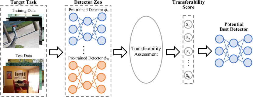
Figure 1: Illustration for selection of pre-trained detectors. The selection is performed by efficient transferability assessment.

To evaluate transferability assessment of object detection, we build up a challenging yet practical experimental setup with a zoo of diverse pretrained detectors. Specifically, we collect $33$ large-scale pre-trained object detectors including two-stage [43, 4], single-stage [35, 50], and transformer [70, 12] based detection architectures. Meanwhile, they are equipped with different backbones, varying in ResNets [25], ResNeXts [58], and RegNets [42] and pre-trained with various datasets [36, 32, 13]. Moreover, we adopt $6$ downstream tasks from $5$ diverse domains under different scenarios including general objects [16], driving [10, 23], dense prediction [46], Unmanned Aerial Vehicle (UAV) [69] and even medical lesions [60]. In contrast, previous classification assementment methods usually simultaneously rank over 10$\sim$20 pretrained models and test on datasets from at most 3 domains [38, 14, 40]. Upon the detection transferability benchmark, we propose to assess classification and regression sub-tasks simultaneously in a unified framework. Moreover, a complementary metric is designed for better assess tasks with various object scales.

Our main contributions are summarized as:

• This paper studies a crucial yet underexplored problem: efficient transferability assessment of pre-trained detectors.

• We build up a challenging detection transferability benchmark, containing $33$ pre-trained detectors with different architectures, different source datasets and training schemes, and evaluating on diverse downstream target tasks. A series of metrics are designed to effectively assess these pre-trained detectors.

• Extensive experimental results upon this challenging transferability benchmark show the effectiveness and robustness of the proposed assessment framework compared with previous SOTA methods. Most importantly, it achieves over $32\times$ wall-clock time speedup and only $5.2\%$ memory footprint requirement compared with brute-force fine-tuning.

2 Related Work

2.1 Transferability of Pre-trained Models

Assessing the transferability of pre-trained models is an essential and crucial task. Early works [63, 30] have studied the transferability of the neural networks based on various layers within a single model and various models within a model zoo while the conclusions were drawn from too expensive fine-tuning (see Sec. 5.4), which is not affordable. Further, the transferability of deep knowledge was studied by evaluating the task relatedness [66, 15, 54, 52] and building attribution graphs [48, 49]. But these solutions still need costly downstream training and they are not applicable when meeting multi-scale features, multiple sub-tasks, and diverse detection heads, which are the key components in object detection.

Recently, several papers introduced efficient transferability metrics for classification. LEEP [38] proposed to efficiently evaluate the transferability of pre-trained models for supervised classification tasks by calculating the log expectation of the empirical predictor. However, the performance of LEEP degrades when the number of classes within the source data is less than that of the target task. A series of following works [33, 2] further improve LEEP for multi-class classification and pixel-level classification (i.e., semantic segmentation). $\mathcal{N}$-LEEP [33] tried to improve LEEP with Principal Component Analysis on the model outputs. and established a neural checkpoint ranking benchmark for classification. To better assess multi-class classification, Ding et al.[14] proposed a series of Cross Entropy (CE) based metrics for pre-trained classification models. Pándy et al.[40] proposed to estimate the pairwise Gaussian class separability using the Bhattacharyya coefficient, which could be applicable for both classification and segmentation. In SFDA [47], the authors aimed to leverage the fine-tuning dynamics into transferability measurement in a self-challenging fisher space, which degraded the efficiency.

Different from previous works designed for image-level or pixel-level classification, this paper aims to tackle more challenging pre-trained detector assessment. We thus build up a detector transferability benchmark, which simultaneously ranks 33 pre-trained models over 6 target datasets from 5 diverse domains, comparing with $10\!\!\!\!\sim\!\!\!\!20$ pre-trained models and 3 target domains in classification scenarios. Moreover, assessing pre-trained detectors should consider both classification and regression sub-tasks together. LogME [64, 65] first extends the transferability assessment from classification to regression and thus can be used as a baseline to assess the transferability of pre-trained detectors. However, it is designed for general regression task, without considering the multi-scale characteristics and inherent relation between coordinates in bounding box regression sub-task. To address these issues, we extend LogME to a series of metrics with special design for object detection.

2.2 Object Detection

Object detection is a practical computer vision task that aims to detect the objects and recognize the corresponding classes from an input image. The object detectors are always trained under supervised [43, 4, 35, 53, 70] and self-supervised [56, 61, 12, 3] schemes on the large-scale datasets [36, 32, 22, 45, 13]. The supervised detectors are trained with ground truth bounding boxes and class labels while the self-supervised ones can only access the training images. Regarding the design of different detection architectures, there are three main streams, including two-stage [43, 4, 67], single-stage [35, 53, 50], and transformer [70, 12, 3] based detectors. A typical two-stage detector [43] works with $1$st-stage proposal generator and $2$nd stage bounding box refinement and class recognition while a single-stage detector [35] aims to perform dense predictions for the object location and class. Recent transformer based end-to-end detectors [5, 70] consider the object detection task as a direct set prediction problem optimized with Hungarian algorithm [31], in which lots of human-designed complex components are removed. With these large-scale pre-trained object detectors, how to figure out a good one for a given downstream detection task is crucial but underexplored. In this work, we aim to tackle the efficient transferability assessment for pre-trained detectors, which infers the true fine-tuning performance on a give downstream task.

3 Detector Transferability Benchmark

In this work, we construct a zoo of different detectors pre-trained with various source datasets and and thus build up a transferability benchmark to measure different assessment metrics. In what follows, we will provide details of the detector transferability benchmark.

Problem Setup.

With a given downstream detection task and a detection model zoo consisting of $N$ pre-trained models $\{\mathcal{F}_{n}\}_{n=1}^{N}$, the aim of model transferability assessment is to produce a transferability score for every pre-trained detector, and then find the best one for further fine-tuning according to the score ranking.

Table 1: Pre-training schemes, source datasets and detection architectures used in this work. We include two-stage, single-stage, and transformer based detectors to build a pre-trained detector zoo. These detectors are equipped with different backbones, e.g., ResNets [25], ResNeXts [58], and RegNets [42].

Scheme	Dataset	Type	Detector	Backbone
Supervised	COCO [36]	two-stage	FRCNN [43]	R50 [25] [t]
				R101 [25]
				X101-32x4d [25]
				X101-64x4d [25] [b]
			Cascade RCNN [4]	R50 [25] [t]
				R101 [25]
				X101-32x4d [25]
				X101-64x4d [25] [b]
			Dynamic RCNN [67]	R50 [25]
			RegNet [42]	400MF [42] [t]
				800MF [42]
				1.6GF [42]
				3.2GF [42]
				4GF [42] [b]
			DCN [11]	R50 [25] [t]
				R101 [25]
				X101-32x4d [25] [b]
		single-stage	FCOS [53]	R50 [25] [t]
				R101 [25] [b]
			RetinaNet [35]	R18 [25] [t]
				R50 [25]
				R101 [25]
				X101-32x4d [25]
				X101-64x4d [25] [b]
			Sparse RCNN [50]	R50 [25] [t]
				R101 [25] [b]
		transformer	DDETR [70]	R50 [25]
	Open Images [32]	two-stage	FRCNN [43]	R50 [25]
		single-stage	RetinaNet [35]	R50 [25]
Self- Supervised	ImageNet [13]	two-stage	SoCo [56]	R50 [25] [t]
			InsLoc [61]	R50 [25] [b]
		transformer	UP-DETR [12]	R50 [25] [t]
			DETReg [3]	R50 [25] [b]

Pre-trained Source Detectors.

In the past few years, a great number of detection models arise with very smart design. Typically, these detectors are trained under supervised [43, 53, 70] or self-supervised [56, 12] scenarios. Supervised detectors are always trained and evaluated on large-scale detection datasets, such as COCO [36] and Open Images [32], while self-supervised ones are trained based on ImageNet [13]. In this work, we take three datasets, i.e., COCO, Open Images, and ImageNet, as the source datasets for different pre-training schemes. Upon these source datasets and training schemes, we use $13$ detection architectures, including two-stage [43, 4, 67, 42, 11, 56, 61], single-stage [35, 53, 50], and transformer [70, 12, 3] based detectors, for pre-training and obtain a model zoo composed of $33$ various pre-trained detectors. These detectors are equipped with different backbones, e.g., ResNets [25], ResNeXts [58], and RegNets [42]. The detailed information is shown in Table 1. With a large variety of pre-trained source detectors, it can be ensured that at least one good model exists for a given target task and our evaluation metric can distinguish between bad and good source models.

Target Datasets.

The image domain plays an important role for deep-learning-based models, which directly determines the model performance in a transfer learning scenario [39, 37]. So we cover a wide range of image domains as a challenging but practical setting with diverse scenarios, including general objects [16], driving [10, 23], dense prediction [46], Unmanned Aerial Vehicle (UAV) [69], and even medical lesions [60]. The detailed information of these target datasets are summarized in Table 2.

Table 2: Target downstream datasets used in this work, in which they are from $5$ diverse domains.

Dataset	Domain	Classes	Images
Pascal VOC [16]	General	20	21K
CityScapes [10]	Driving	8	5K
SODA [23]	Driving	6	20K
CrowdHuman [46]	Dense	1	24K
VisDrone [69]	UAV	11	9K
DeepLesion [60]	Medical	8	10K

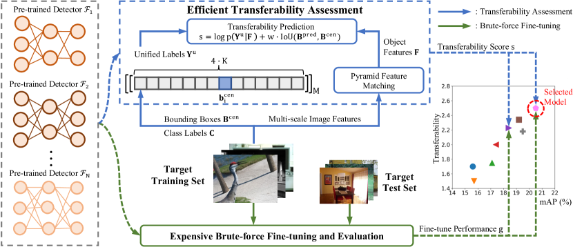
Figure 2: The overview of efficient transferability assessment framework for pre-trained detection models. We build a challenging setting contains various pre-trained object detectors. Based on this challenging setting, we design a pyramid feature matching scheme to handle objects with various sizes and expand the bounding box matrix $\boldsymbol{B}^{cen}$ according to class label matrix $\boldsymbol{C}$ to the unified label matrix $\boldsymbol{Y}^{u}$ for evaluation. We estimate the maximum evidence $p(\boldsymbol{Y}^{u}|\boldsymbol{F})$, which indicates the compatibility between the object features $\boldsymbol{F}$ and unified labels $\boldsymbol{Y}^{u}$. Further, considering IoU as an important metric in object detection, we supply IoU between the predicted bounding boxes and ground truth ones as a complementary term for transferability assessment of detection model.

Evaluation Protocol.

Given pre-trained object detectors $\{\mathcal{F}_{n}\}_{n=1}^{N}$ and a downstream dataset $\mathcal{D}_{t}$, a transferability assessment method will produce the transferability scores $\{s_{n}\}_{n=1}^{N}$. Following the previous works [33, 64, 2, 40, 47, 14, 65], we take the fine-tuning performance of pre-trained detectors $\{g_{n}\}_{n=1}^{N}$ as the ground truth, i.e., mean Average Precision (mAP) as the metric in object detection. Ideally, the transferability scores are positively correlated with true fine-tuning performance. That is, if a pre-trained model $\mathcal{F}_{n}$ has higher detection mAP than $\mathcal{F}_{m}$ after fine-tuning ($g_{n}\textgreater g_{m}$), the transferability score of $\mathcal{F}_{n}$ is also expected to be larger than $\mathcal{F}_{m}$ ($s_{n}\textgreater s_{m}$). So the effectiveness of a transferability metric for assessing the pre-trained detectors is evaluated by the ranking correlation between the ground truth fine-tuning performance $\{g_{n}\}_{n=1}^{N}$ and estimated transferability scores $\{s_{n}\}_{n=1}^{N}$. We use Weighted Kendall’s $\tau_{w}$ [27] as the evaluation metric. Larger $\tau_{w}$ indicates better ranking correlation between $\{g_{n}\}_{n=1}^{N}$ and $\{s_{n}\}_{n=1}^{N}$ and better transferability metric. $\tau_{w}$ is interpreted by

$$\small\tau_{w}=\frac{2}{N(N-1)}\!\!\sum_{1\leq n<m\leq N}\!\!\operatorname{sgn}\left(g_{n}-g_{m}\right)\operatorname{sgn}\left(s_{n}-s_{m}\right).$$ (1)

Here $\tau_{w}$ ranges in $[-1,1]$, and the probability of $g_{n}\textgreater g_{m}$ is $\frac{\tau_{w}+1}{2}$ when $s_{n}\textgreater s_{m}$. Moreover, we use Top-1 Relative Accuracy (Rel@1) [33] to measure how close model with the highest transferability performs, in terms of fine-tuning performance, compared to the highest performing model.

4 Detection Model Transferability Metrics

In this section, we study the problem of efficient transferability assessment for detection model. Given a model zoo with a number of pre-trained detectors and a target downstream task, our goal is to predict their transferability performance on the target task efficiently, without brute-force fine-tuning all pre-trained models. LogME is a classification assessment method designed from the viewpoint of regression [64]. Thus, it can be used to assess transferability of pre-trained detectors which contain both classification and regression subtasks. However, it is designed for general regression and might fail when tackling the bounding box regression task with multi-scale characteristics of inputs and inherent relation between coordinates in outputs. To this end, as shown in Figure 2, we extend LogME to detection scenario by designing a unified framework (U-LogME in Sec. 4.2) which assesses multiple sub-tasks and multi-scale features simultaneously. Furthermore, we propose a complementary metric (i.e., IoU-LogME in Sec. 4.3) for better transferability assessment over objects with varying scales.

4.1 LogME as a Basic Metric

Different from most existing assessment methods that measure class separation of visual features, LogME addresses the problem from the viewpoint of regression. Specifically, it uses a set of Bayesian linear models to fit the features extracted by the pre-trained models and the corresponding labels. The marginalized likelihood of these linear models is used to rank pre-trained models. Since it can address both classification and regression tasks, we can easily extend it to assess object detection framework.

Specifically, we extract multi-scale object-level features of ground-truth bounding boxes by using pre-trained detectors’ backbone followed by an ROIAlign layer [43]. In this way, for a given pre-trained detector and a downstream task, we can collect the object-level features of downstream task by using the detector and form a feature matrix $\boldsymbol{F}$, with each row $\boldsymbol{f}_{i}$ denotes an object-level feature vector. For each $\boldsymbol{f}_{i}$, we also collect its 4-d coordinates of ground-truth bounding box $\boldsymbol{b}_{i}$ and class label $c_{i}$ to form a bounding box matrix $\boldsymbol{B}$ and a class label matrix $\boldsymbol{C}$.

For the bounding box regression sub-task, LogME measures the transferability by using the maximum evidence $p(\boldsymbol{B}|\boldsymbol{F})\!\!=\!\!\int p(\boldsymbol{\theta}|\alpha)p(\boldsymbol{B}|\boldsymbol{F},\beta,\boldsymbol{\theta})d\boldsymbol{\theta}$, where $\boldsymbol{\theta}$ is the parameter of linear model. $\alpha$ denotes the parameter of prior distribution of $\boldsymbol{\theta}$, and $\beta$ denotes the parameter of posterior distribution of each observation $p(\boldsymbol{b}_{i}|\boldsymbol{f}_{i},\beta,\boldsymbol{\theta})$. By using the evidence theory [28] and basic principles in graphical models [29], the transferability metric can be formulated as

$$\operatorname{LogME}= \log p(\boldsymbol{B}|\boldsymbol{F})$$ (2)

$$= \frac{M}{2}\log\beta+\frac{D}{2}\log\alpha-\frac{M}{2}\log 2\pi$$

$$-\frac{\beta}{2}\|\boldsymbol{F}\boldsymbol{m}-\boldsymbol{B}\|_{2}^{2}-\frac{\alpha}{2}\boldsymbol{m}^{T}\boldsymbol{m}-\frac{1}{2}\log|A|,$$

where $\boldsymbol{m}$ is the solution of $\boldsymbol{\theta}$, $M$ is the number of objects, $D$ is the dimension of features, and $A$ is the $L_{2}$-norm of $\boldsymbol{F}$.

LogME for classification sub-task can be computed by replacing $\boldsymbol{B}$ in Eq. (2) with converted one-hot class label matrix. By combining the evidences of two sub-tasks together, we obtain a final evidence for ranking the pre-trained detector. However, LogME still struggles to rank the pre-trained detectors accurately due to the following four challenges: 1) The single-scale features of LogME is not compatible with the multi-scale features extracted by pyramid network architecture of pre-trained detector. 2) The huge coordinates variances of different-scale objects make it hard to fit by simple linear model used in LogME. 3) The assessment branch of classification sub-task might fail when the downstream task is single-class detection. 4) The mean squared error (MSE) used in LogME isn’t scale-invariant and measures each coordinate separately, which is not suitable for bounding box regression. In what follows, we propose how to address these issues.

4.2 U-LogME

This subsection proposes to unify multi-scale features and multiple tasks into an assessment framework. Here, we propose a pyramid feature mapping scheme to extract suitable features for different scale objects. Meanwhile, we normalize coordinates of bounding boxes and jointly evaluate 4-d coordinates with the same linear network. This can help to reduce coordinate variances and thus benefit ranking. Furthermore, we merge the class labels and normalized bounding box coordinates into a final ground-truth label to joint assess two sub-tasks with the same model. In this way, both single-class and multiple-class downstream detection tasks are unified into one assessment framework. We provide more technical details in the following.

Pyramid Feature Matching.

Classical object detectors always include a Feature Pyramid Network (FPN) [34] like architecture with different feature levels. The object features are obtained from different levels according to the corresponding object sizes during training, e.g., very small and large objects will be mapped to bottom-level and top-level image features, respectively. Regarding this, we introduce pyramid feature matching to help objects with different sizes find their matched level features. Following FPN [34], we assign an object to the feature pyramid level $P_{l}$ by the following:

$$\small l=\left\lfloor l_{0}+\log_{2}(\sqrt{wh}/224)\right\rfloor,$$ (3)

where $w$ and $h$ is the width and length of an object on the input image to the network, respectively. Here $224$ is the ImageNet [13] training size, and $l_{0}$ is the feature level mapped by an object with $w\!\times\!h\!=\!224^{2}$. Inspired by FCOS [53], to better handle too small and large objects, objects satisfying $\max(w,h)\textless 64$ and $\max(w,h)\textgreater 512$ are further forcibly assigned to the lowest and highest level of feature pyramid. Given a bounding box and its $P_{l}$, we use an RoI Align layer to crop the $P_{l}$-th feature map according to bounding box coordinates and thus obtain its features. Thus, we can extract suitable visual features for multi-scale ground-truth objects.

Improved BBox Evaluation.

With these multi-scale object features, our model can predict their coordinates of bounding boxes. In the object detection scenario, bounding box targets can be formulated as corner-wise coordinates $\boldsymbol{b}_{i}\!=\!(x_{1},y_{1},x_{2},y_{2})$ or center-wise coordinates $\boldsymbol{b}^{cen}_{i}\!\!=\!\!(x_{c},y_{c},w_{c},h_{c})$. To avoid coordinate scale issue, each coordinate is rescaled to the range [0,1] by using bounding box center normalization. Since the bias in the former one (i.e., $x_{1}<x_{2},y_{1}<y_{2}$) is hard to be fit by a linear model in LogME, we thus select the latter one. LogME for bounding box regression is obtained by averaging over $4$-d coordinates, where each coordinate learns different prior distribution with different $\alpha$ and $\beta$. Considering the inherent relation between coordinates, we feed $4$-d coordinates of a bounding box as a whole and learn a shared prior distribution for 4 coordinates with the same $\alpha$ and $\beta$. More specifically, We expand the dimension of $\boldsymbol{m}$ in Eq. (2) from $\boldsymbol{m}\!\!\in\!\!\mathbb{R}^{D}$ to $\boldsymbol{m}\!\!\in\!\!\mathbb{R}^{D\!\times\!4}$ to match the dimension of $\boldsymbol{B}^{cen}$, resulting in a more efficient and accurate evaluation.

Table 3: Ranking results of of six methods for 1% 33-choose-22 possible source model sets (over 1.9M) on $6$ downstream target datasets. Higher $\tau_{w}$ and Rel@1 indicate better ranking and transferability metric. As SFDA is specifically designed for classification task, it is not applicable for the single-class task of CrowdHuman. The results of all three variants of our approach, U-LogME, IoU-LogME, and Det-LogME are reported. The best methods are in red and good ones are in blue.

Measure	Weighted Kendall’s tau ($\tau_{w}$) $\uparrow$						Top1 Relative Accuracy (Rel@1) $\uparrow$
Method	KNAS	SFDA	LogME	U-LogME	IoU-LogME	Det-LogME	KNAS	SFDA	LogME	U-LogME	IoU-LogME	Det-LogME
Pascal VOC	0.10$\pm$0.18	0.65$\pm$0.13	0.15$\pm$0.22	0.40$\pm$0.17	0.58$\pm$0.16	0.78$\pm$0.03	0.94$\pm$0.10	1.00$\pm$0.00	0.91$\pm$0.12	0.96$\pm$0.05	1.00$\pm$0.00	1.00$\pm$0.00
CityScapes	-0.22$\pm$0.24	0.45$\pm$0.06	0.15$\pm$0.20	0.13$\pm$0.16	0.51$\pm$0.09	0.57$\pm$0.08	0.95$\pm$0.06	0.95$\pm$0.01	0.95$\pm$0.06	0.90$\pm$0.04	0.98$\pm$0.02	0.98$\pm$0.02
SODA	-0.46$\pm$0.09	0.46$\pm$0.12	0.13$\pm$0.21	0.04$\pm$0.17	0.61$\pm$0.09	0.61$\pm$0.09	0.88$\pm$0.04	0.95$\pm$0.02	0.92$\pm$0.11	0.87$\pm$0.06	0.98$\pm$0.02	0.98$\pm$0.02
CrowdHuman	-0.42$\pm$0.11	N/A	0.19$\pm$0.19	0.21$\pm$0.18	0.34$\pm$0.16	0.34$\pm$0.16	0.85$\pm$0.04	N/A	0.97$\pm$0.04	0.97$\pm$0.04	0.98$\pm$0.03	0.98$\pm$0.03
VisDrone	0.04$\pm$0.20	0.53$\pm$0.12	0.48$\pm$0.17	0.17$\pm$0.17	0.70$\pm$0.08	0.69$\pm$0.08	0.88$\pm$0.17	1.00$\pm$0.00	0.90$\pm$0.15	0.78$\pm$0.13	0.99$\pm$0.02	0.99$\pm$0.02
DeepLesion	-0.13$\pm$0.19	-0.21$\pm$0.14	0.08$\pm$0.20	0.52$\pm$0.14	-0.05$\pm$0.18	0.42$\pm$0.17	0.69$\pm$0.11	0.65$\pm$0.06	0.72$\pm$0.17	0.87$\pm$0.28	0.64$\pm$0.07	0.75$\pm$0.38
Average	-0.18$\pm$0.28	0.31$\pm$0.10	0.19$\pm$0.20	0.24$\pm$0.17	0.45$\pm$0.13	0.57$\pm$0.10	0.86$\pm$0.09	0.91$\pm$0.02	0.90$\pm$0.11	0.89$\pm$0.10	0.93$\pm$0.03	0.95$\pm$0.08

Unified Sub-task Evaluation.

Although the correlations among the coordinates are captured by joint evaluation of bounding box coordinates, LogME for regression sub-task still suffers from neglecting object classes information. So how to build the correlation between these sub-tasks? Inspired by the class-aware detection heads of classical detectors [43, 53, 70], we propose unified sub-task evaluation for assessing the transferability of pre-trained detectors. To be specific, we combine the bounding box matrix $\boldsymbol{B}^{cen}$ and class label matrix $\boldsymbol{C}$ as the unified label matrix $\boldsymbol{Y}^{u}$. The bounding box matrix $\boldsymbol{B}^{cen}$ is expanded from $\boldsymbol{B}^{cen}\!\!\in\!\!\mathbb{R}^{M\!\times\!4}$ to $\boldsymbol{Y}^{u}\!\!\in\!\!\mathbb{R}^{M\!\times\!(4\cdot K)}$ according to $\boldsymbol{C}$, where $K$ is the total number of classes. By integrating pseudo bounding boxes filled with $0$ coordinates, we obtain unified label matrix $\boldsymbol{Y}^{u}$ as

$$\centering\small\boldsymbol{Y}^{u}\!\!=\!\!\left[\!\left[\!\underbrace{(0,0,0,0)}_{1\operatorname{st}},\dots\!,\overbrace{\underbrace{\left(x_{c},y_{c},w_{c},h_{c}\right)}_{c_{i}\operatorname{-th}}}^{\boldsymbol{b}_{i}^{cen}},\dots\!,\underbrace{(0,0,0,0)}_{K\operatorname{-th}}\!\right]\!\right]_{M}\!\!\!.\@add@centering$$ (4)

To this end, both bounding boxes and classes information are represented by $\boldsymbol{Y}^{u}$. Accordingly, $\boldsymbol{m}$ in Eq. (2) is further expanded from $\boldsymbol{m}\!\!\in\!\!\mathbb{R}^{D\!\times\!4}$ to $\boldsymbol{m}\!\!\in\!\!\mathbb{R}^{D\!\times\!(4\cdot K)}$ for matching the dimension of $\boldsymbol{Y}^{u}$. We can take the unified label matrix $\boldsymbol{Y}^{u}$ as the input for transferability assessment and obtain a unified transferability score for detection as the following:

$$\small\operatorname{U-LogME}=\log p(\boldsymbol{Y}^{u}\!\mid\!\boldsymbol{F}).$$ (5)

4.3 IoU-LogME

Although U-LogME addressed multi-scale and multi-task issues of vanilla LogME, the MSE used for fitting features and bounding box coordinates is not robust to object scales. That is, the larger objects might cause bigger MSE, which makes the model prefers larger objects than smaller ones. Moreover, each coordinate is evaluated separately in mean squared error, without considering the correlations between different coordinates. To overcome this issue, we introduce IoU metric into U-LogME. Specifically, $\boldsymbol{m}$ in Eq. (2) is interpreted as a linear regression model so that $\boldsymbol{F}\boldsymbol{m}$ can be regarded as the bounding box predictions from a detector naturally. We propose to calculate the IoU between the bounding boxes predictions $\boldsymbol{F}\boldsymbol{m}$ and the corresponding ground truth bounding boxes $\boldsymbol{B}^{cen}$ as a IoU based transferability measurement. Considering $\boldsymbol{m}\!\!\in\!\!\mathbb{R}^{D\times(4\cdot K)}$ is computed from the unified label matrix $\boldsymbol{Y}^{u}\!\!\in\!\!\mathbb{R}^{M\times(4\cdot K)}$ in Eq. (4), so we downsample $\boldsymbol{m}$ to $\boldsymbol{m}^{\prime}\!\!\in\!\!\mathbb{R}^{D\times 4}$ by reserving the values where real coordinates of $\boldsymbol{B}^{cen}$ arise. This IoU-based metric is formulated as:

$$\small\operatorname{IoU-LogME}=\operatorname{IoU}(\boldsymbol{F}\boldsymbol{m}^{\prime},\boldsymbol{B}^{cen})=\frac{|\boldsymbol{F}\boldsymbol{m}^{\prime}\cap\boldsymbol{B}^{cen}|}{|\boldsymbol{F}\boldsymbol{m}^{\prime}\cup\boldsymbol{B}^{cen}|}.$$ (6)

4.4 Det-LogME

Although IoU-LogME is invariant to objects with different scales, it degrades to 0 when the two inputs have no intersection and fails to measure the absolute difference between them. On the contrary, MSE is good at tackling these cases. Therefore, to take advantage of their strengths, we propose to combine them together and obtain a final detector assessment metric $\operatorname{Det-LogME}$, which is formulated as:

$$\small\operatorname{Det-LogME}=\operatorname{U-LogME}+\mu\cdot\operatorname{IoU-LogME},$$ (7)

where $\mu$ is used for controlling the weight of IoU. $\operatorname{U-LogME}$ and $\operatorname{IoU-LogME}$ are normalized to $[0,1]$ upon 33 pre-trained detectors to unify the scale.

5 Experiment

5.1 Experimental Setup

We employ the proposed benchmark in Sec. 3 to conduct experiments. Our method is compared with KNAS [59], SFDA [47], and LogME [64]. KNAS is a gradient-based approach that operates under the assumption that gradients can predict downstream training performance. Therefore, we use it as a point of comparison with our efficient gradient-free approach. SFDA is not applicable for the single-class task of CrowdHuman [46]. Therefore, we present the SFDA results on five other multiple-class datasets. It is worth noting that our proposed pyramid feature matching enhances both LogME and SFDA, facilitating their evaluation. Furthermore, we present results for all three variants of our approach: U-LogME, IoU-LogME, and Det-LogME. We utilize two evaluation measures, namely the ranking correlation Weighted Kendall’s tau ($\tau_{w}$), as defined in Eq. (1), and the Top-1 Relative Accuracy (Rel@1). Larger values of $\tau_{w}$ and Rel@$1$ indicate better assessment results.

5.2 Main Results

As discussed in [1], transferability metrics can be unstable. To address this issue, we randomly sub-sample 22 models from 33 pre-trained detectors and use 1% of the 33-choose-22 possible source model sets (over 1.9M) for measurement, as shown in Table 3. Our observations indicate that KNAS performs poorly on all 6 target datasets, with negative ranking correlation $\tau_{w}$. Our method Det-LogME consistently outperforms LogME on 6 downstream tasks. For instance, Det-LogME surpasses LogME by substantial margins of $0.63$, $0.48$, and $0.34$ in terms of ranking correlation $\tau_{w}$ on Pascal VOC, SODA, and DeepLesion, respectively. This validates the high effectiveness of our proposed unified evaluation and complementary IoU measurement. On five multiple-class downstream datasets, Det-LogME still outperforms classification-specific SFDA, particularly on DeepLesion ($+0.63\ \tau_{w}$). This further indicates that classification-specific transferability metrics may not yield optimal results for multi-class detection problems. Furthermore, our Det-LogME achieves better Rel@1 values than all other SOTA methods in average, outperforming the second-best method SFDA by 4% top-1 relative accuracy. Overall, our method is robust and consistently outperforms competing methods over 1.9M sub-sampled model sets.

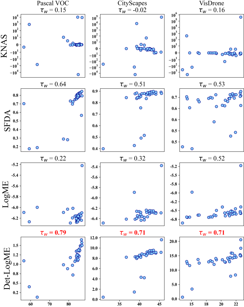
Figure 3: Comparison of ranking scores. The plots illustrate ground-truth fine-tuning performance $\{g_{n}\}_{n=1}^{N}$ (x-axis), ranking scores (y-axis), and Weighted Kendall’s coefficient $\tau_{w}$ for 33 pre-trained detectors on 3 out of 6 target datasets.

Regarding the three variants proposed in this paper, U-LogME performs the worst in most cases. We have further observations to make. On one hand, IoU-LogME, which uses IoU as a scale-invariant metric, performs better than MSE-based U-LogME in scenarios where the objects vary greatly in scale. This is especially evident in CityScapes [10], SODA [23], and VisDrone [69], where objects captured under driving or UAV scenarios have diverse scales. On the other hand, IoU-based IoU-LogME suffers from the problem of remaining equal to $0$ when there is no intersection between the predicted and ground truth bounding boxes, regardless of how far apart they are. In contrast, MSE-based U-LogME can handle this problem with absolute distances. This is particularly evident in DeepLesion [60], where the lesions are very small and difficult to detect. Det-LogME, which combines the advantages of both unified evaluation and IoU measurement, achieves a trade-off and better ranking performance than U-LogME and IoU-LogME. We can also observe that Det-LogME performs better on five multiple-class tasks than the single-class one. This indicates the significant difficulties and challenges involved in evaluating the pre-trained detectors on dense tasks.

Figure 3 illustrates the relationship between predicted transferability and actual fine-tuning performance of 33 pre-trained detectors for our Det-LogME and three SOTA methods on three target datasets. We observe that our Det-LogME consistently shows better positive correlations compared to other SOTA methods in all experiments, which demonstrates the effectiveness of our proposed approach.

5.3 Ablation Studies

In this subsection, we carefully study our proposed Det-LogME with respect to different components and hyper-parameters by assessing $33$ detectors on the Pascal VOC.

Components Analysis of Det-LogME.

As shown in Table 5, we can learn that the large variances of different coordinates are eliminated by bounding box center normalization and the ranking correlation $\tau_{w}$ is improved $0.11$. By jointly evaluating $4$-d coordinates, $\tau_{w}$ improves from $0.33$ to $0.40$, indicating the inherent correlations among $4$ coordinates within a bounding box are captured by our proposed joint evaluation. Under unified sub-task evaluation, $\tau_{w}$ further improves from $0.40$ to $0.43$, which demonstrates the effectiveness of unifying the supervision information by considering object classes information. Finally, we observe that the inclusion of the complementary IoU metric in our evaluation framework leads to a substantial increase in ranking performance from 0.43 to 0.79 ($+0.36\ \tau_{w}$). This finding underscores the importance of IoU measurement in assessing the transferability of pre-trained detectors.

Table 4: Effects of different components of Det-LogME.

Method	$\tau_{w}$ $\uparrow$
Baseline (LogME)	0.22
w/ bbox center norm.	0.33
w/ joint eval. of coord.	0.40
w/ unified sub-task eval.	0.43
w/ IoU (Det-LogME)	0.79

Table 5: Effects of different bounding box normalization techniques (border and center) in Det-LogME.

Method	$\tau_{w}$ $\uparrow$
Baseline (LogME)	0.22
w/ bbox border norm.	0.22
w/ bbox center norm.	0.33

Table 6: Efficiency evaluation of Det-LogME and comparison with brute-force fine-tuning, naive feature extraction, KNAS, SFDA, and LogME. Note that the wall-clock time and memory footprint for SFDA are evaluated on $5$ multiple-class downstream detection datasets.

Measure	Wall-clock Time (s) $\downarrow$						Memory Footprint (GB) $\downarrow$
Method	Fine-tune	Extract feature	KNAS	SFDA	LogME	Det-LogME	Fine-tune	Extract feature	KNAS	SFDA	LogME	Det-LogME
	(upper bound)	(lower bound)					(upper bound)	(lower bound)
Pascal VOC	28421.09	128.88	129.99	130.14	130.18	129.89	13.39	0.47	13.86	0.55	0.59	0.66
CityScapes	73973.09	50.50	51.53	52.02	51.80	51.18	22.36	0.99	23.34	1.06	1.08	1.10
SODA	13928.24	50.75	51.89	51.88	51.83	51.19	12.54	0.50	13.04	0.54	0.55	0.55
CrowdHuman	43297.45	170.38	171.48	N/A	178.26	175.06	27.24	0.63	27.87	N/A	1.47	1.46
VisDrone	14067.15	63.38	64.51	69.08	68.16	64.97	16.69	0.65	17.34	0.79	0.80	0.84
DeepLesion	8465.45	37.13	38.24	37.49	37.71	37.34	6.99	0.52	7.51	0.53	0.54	0.54
Average	30358.75	83.50	84.60	68.12	86.32	84.94	16.53	0.63	17.16	0.69	0.84	0.86

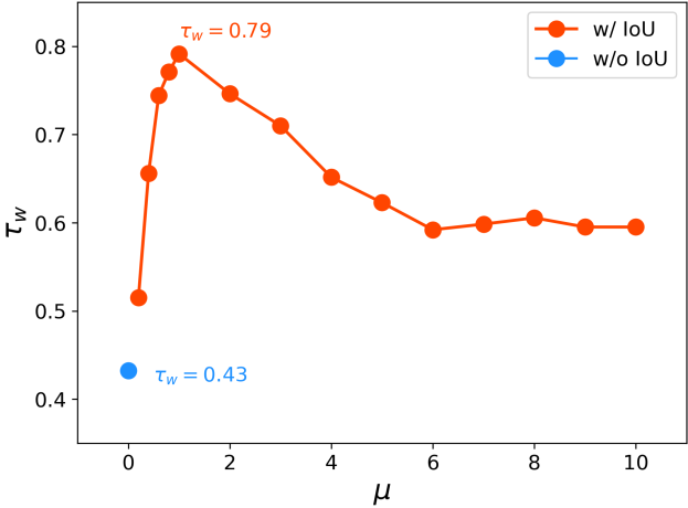
Figure 4: Effects of different weights $\mu$ for complementary IoU metric in Det-LogME. The first blue marker indicates Det-LogME without IoU measurement (degrades to U-LogME).

Different BBox Normalization Techniques.

To mitigate the detrimental effects of large variances among different coordinates, we introduce bounding box normalization. We experiment with two widely used normalization techniques in detection. Except for center normalization described in Section 4.2, we also try to apply border normalization by dividing the bounding box with the corresponding width and height of the input image to obtain $\boldsymbol{b}^{bor}_{i}\!\!=\!\!(x_{1}^{\prime},y_{1}^{\prime},x_{2}^{\prime},y_{2}^{\prime})$. From the results shown in Table 5, we observe that border normalization yields no improvement, and center normalization outperforms it by $+0.1\ \tau_{w}$. Center normalization scales the four coordinates of the bounding box to the same range in $[0,1]$, while border normalization may not work well when significant biases exist among the $x$-axis and $y$-axis coordinates, such as when an object is located near the top-right corner of an image where $x_{1}\gg y_{1}$ or $x_{2}\gg y_{2}$.

Weight of Complementary IoU Metric.

The weight hyper-parameter $\mu$ in Eq. (7) controls the behavior of the complementary IoU metric. Similar to the weights of IoU-related losses [44, 68], the weight $\mu$ is crucial to the final transferability score of Det-LogME. We investigate the effects of different weights $\mu\!\!\in\!\!\{0,0.2,\dots,0.8,1,2,\dots,10\}$ of the IoU metric, and the results are presented in Figure 4. We observe that incorporating the IoU metric as a complementary term consistently improves the ranking performance of Det-LogME compared to not including it (the first blue marker, which degrades to U-LogME, with $\tau_{w}=0.43$). The best ranking performance of Det-LogME is achieved when the weight is $1$, resulting in $\tau_{w}=0.79$.

5.4 Efficiency Analysis

In this subsection, we present a comprehensive evaluation of the assessing efficiency of Det-LogME and compare it with brute-force fine-tuning, naive feature extraction, KNAS, SFDA, and LogME from two perspectives: 1) wall-clock time: the average time of fine-tuning (12 epochs) or evaluating (including feature extraction) all $33$ pre-trained detectors; 2) memory footprint: the maximum memory required during fine-tuning or evaluating (including feature extraction, the loading of all visual features, and computing transferability metric) all $33$ pre-trained detectors. The efficiency of classification-specific SFDA is studied on $5$ multiple-class tasks. The results are presented in Table 6.

Wall-clock Time.

Over 6 downstream tasks, KNAS has the fastest speed, but according to Table 3, it performs the worst, which is not acceptable in practice. On the other hand, with joint evaluation of bounding box coordinates, Det-LogME runs faster than LogME because Det-LogME does not need to evaluate all $4$-d coordinates in a loop. Moreover, Det-LogME runs faster than SFDA, which includes fine-tuning dynamics on all $5$ multiple-class datasets. Considering that the selected model will be fine-tuned on the target task, our proposed Det-LogME brings about $(\operatorname{NumSourceModels}-1)\times$ speedup compared with brute-force fine-tuning, which is $32\times$ in this work.

Memory Footprint.

Table 6 indicates that gradient-based KNAS demands a significant amount of memory exceeding 17 GB, rendering it infeasible for most practical applications. In comparison, Det-LogME only marginally increases the memory when compared to LogME and SFDA, making it practical for deployment. Furthermore, Det-LogME demonstrates high memory efficiency by requiring 19$\times$ less memory than brute-force fine-tuning, underscoring its potential to save computational resources.

6 Conclusion

In this paper, we aim to address a practical but underexplored problem of efficient transferability assessment for pre-trained detection models. To achieve this, we establish a challenging detector transferability benchmark comprising a large and diverse zoo consisting of 33 detectors with various architectures, source datasets and schemes. Upon this zoo, we adopt 6 downstream tasks spanning 5 diverse domains for evaluation. Further, we propose a simple yet effective framework for assessing the transferability of pre-trained detectors. Extensive experimental results demonstrate the high effectiveness and efficiency of our approach compared with other state-of-the-art methods across a wide range of pre-trained detectors and downstream tasks, notably outperforming brute-force fine-tuning in terms of computational efficiency. We hope our work can inspire further research into the selection of pre-trained models, particularly those with multi-scale and multi-task capabilities.

Acknowledgements.

We gratefully acknowledge the support of Mindspore, CANN (Compute Architecture for Neural Networks) and Ascend AI Processor used for this work.

Appendix A LogME Measurement for Object Detection

In this work, we extend a classification assessment method LogME [64] to object detection. In this section, we will give detailed derivations of LogME for object detection framework.

Different from image-level features used for assessing classification task, we extract object-level features of ground-truth bounding boxes by using pre-trained detectors’ backbone followed by an ROIAlign layer [43]. In this way, for a given pre-trained detector and a downstream task, we can collect the object-level features of downstream task by using the detector and form a feature matrix $\boldsymbol{F}$, with each row $\boldsymbol{f}_{i}$ denotes an object-level feature vector. For each $\boldsymbol{f}_{i}$, we also collect its 4-d coordinates of grounding-truth bounding box $\boldsymbol{b}_{i}$ and class label $c_{i}$ to form a bounding box matrix $\boldsymbol{B}$ and a class label matrix $\boldsymbol{C}$.

For the bounding box regression sub-task, LogME measures the transferability by using the maximum evidence $p(\boldsymbol{B}|\boldsymbol{F})\!\!=\!\!\int p(\boldsymbol{\theta}|\alpha)p(\boldsymbol{B}|\boldsymbol{F},\beta,\boldsymbol{\theta})d\boldsymbol{\theta}$, where $\boldsymbol{\theta}$ is the parameter of linear model. $\alpha$ denotes the parameter of prior distribution of $\boldsymbol{\theta}$, and $\beta$ denotes the parameter of posterior distribution of each observation $p(\boldsymbol{b}_{i}|\boldsymbol{f}_{i},\beta,\boldsymbol{\theta})$. By using the evidence theory [28] and basic principles in graphical models [29], the evidence can be calculated as

$$p(\boldsymbol{B}\!\mid\!\boldsymbol{F}) =\int p(\boldsymbol{\theta}|\alpha)p(\boldsymbol{B}|\boldsymbol{F},\beta,\boldsymbol{\theta})d\boldsymbol{\theta}$$ (8)

$$=\int p(\boldsymbol{\theta}\!\mid\!\alpha)\prod^{M}_{i=1}p(\boldsymbol{b}_{i}|\boldsymbol{f}_{i},\beta,\boldsymbol{\theta})d\boldsymbol{\theta}$$

$$=\left(\frac{\beta}{2\pi}\right)^{\frac{M}{2}}\left(\frac{\alpha}{2\pi}\right)^{\frac{D}{2}}\int e^{-\frac{\alpha}{2}\boldsymbol{\theta}^{T}\boldsymbol{\theta}-\frac{\beta}{2}\|\boldsymbol{f}_{i}\boldsymbol{\theta}-\boldsymbol{b}_{i}\|^{2}}\mathrm{~{}d}\boldsymbol{\theta},$$

where $M$ is the number of objects and $D$ is the dimension of object features. When $A$ is positive definite,

$$\small\int e^{-\frac{1}{2}\left(\boldsymbol{\theta}^{T}A\boldsymbol{\theta}+b^{T}\boldsymbol{\theta}+c\right)}\mathrm{d}\boldsymbol{\theta}=\frac{1}{2}\sqrt{\frac{(2\pi)^{D}}{|A|}}e^{\frac{1}{4}b^{T}A^{-1}b-c}.$$ (9)

LogME takes the logarithm of Eq. (8) for simpler calculation. So the transferability score is expressed by

$$\text{LogME}= \log p(\boldsymbol{B}|\boldsymbol{F})$$ (10)

$$= \frac{M}{2}\log\beta+\frac{D}{2}\log\alpha-\frac{M}{2}\log 2\pi$$

$$-\frac{\beta}{2}\|\boldsymbol{F}\boldsymbol{m}-\boldsymbol{B}\|_{2}^{2}-\frac{\alpha}{2}\boldsymbol{m}^{T}\boldsymbol{m}-\frac{1}{2}\log|A|.$$

where $A$ and $m$ are

$$\small A=\alpha I+\beta\boldsymbol{F}^{T}\boldsymbol{F},\boldsymbol{m}=\beta A^{-1}\boldsymbol{F}^{T}\boldsymbol{B},$$ (11)

where $A$ is the $L_{2}$-norm of $\boldsymbol{F}$, and $\boldsymbol{m}$ is the solution of $\boldsymbol{\theta}$. Here $\alpha$ and $\beta$ are maxmized by alternating between evaluating $\boldsymbol{m}$, $\gamma$ and maximizing $\alpha$, $\beta$ with $\boldsymbol{m}$, $\gamma$ fixed [20] as the following:

$$\small\begin{gathered}\gamma=\sum_{i=1}^{D}\frac{\beta\sigma_{i}}{\alpha+\beta\sigma_{i}},\alpha\leftarrow\frac{\gamma}{\boldsymbol{m}^{T}\boldsymbol{m}},\beta\leftarrow\frac{M-\gamma}{\|\boldsymbol{F}\boldsymbol{m}-\boldsymbol{B}\|_{2}^{2}},\end{gathered}$$ (12)

where $\sigma_{i}$’s are singular values of $\boldsymbol{F}^{T}\boldsymbol{F}$. With the optimal $\alpha^{*}$ and $\beta^{*}$, the logarithm maximum evidence $\mathcal{L}\left(\alpha^{*},\beta^{*}\right)$ is used for evaluating the transferability. Considering $\mathcal{L}\left(\alpha^{*},\beta^{*}\right)$ scales linearly with the number of objects $M$, it is normalized as $\frac{\mathcal{L}\left(\alpha^{*},\beta^{*}\right)}{M}$, which is interpreted as the average logarithm maximum evidence of all given object feature matrix $\boldsymbol{F}$ and bounding box matrix $\boldsymbol{B}$. LogME for classification sub-task can be computed by replacing $\boldsymbol{B}$ in Eq. (10) with converted one-hot class label matrix.

Nevertheless, optimizing LogME by Eq. (11) and Eq. (12) is timely costly, which is comparable with brute-force fine-tuning. So LogME further improves the computation efficiency as follows. The most expensive steps in Eq. (11) are to calculate the inverse matrix $A^{-1}$ and matrix multiplication $A^{-1}\boldsymbol{F}^{T}$, which can be avoided by decomposing $\boldsymbol{F}^{T}\boldsymbol{F}$. The decomposition is taken by $\boldsymbol{F}^{T}\boldsymbol{F}=V\operatorname{diag}\{\sigma\}V^{T}$, where $V$ is an orthogonal matrix. By taking $\Lambda=\operatorname{diag}\{(\alpha+\beta\sigma)\}$, $A$ and $A^{-1}$ turn to $A=\alpha I+\beta\boldsymbol{F}^{T}\boldsymbol{F}=V\Lambda V^{T}$ and $A^{-1}=V\Lambda^{-1}V^{T}$. With associate law, LogME takes a fast computation by $A^{-1}\boldsymbol{F}^{T}\boldsymbol{B}=\left(V\left(\Lambda^{-1}\left(V^{T}\left(\boldsymbol{F}^{T}\boldsymbol{B}\right)\right)\right)\right)$. To this end, the computation of $\boldsymbol{m}$ in Eq. (11) is optimized as

$$\small\boldsymbol{m}=\beta\left(V\left(\Lambda^{-1}\left(V^{T}\left(\boldsymbol{F}^{T}\boldsymbol{B}\right)\right)\right)\right).$$ (13)

Algorithm 1 Det-LogME

Input: pre-trained detector $\mathcal{F}$, target dataset $\mathcal{D}_{t}$
Output: estimated transferability score $\operatorname{Det-LogME}$

1:Extract multi-scale object-level features using pre-trained detector $\mathcal{F}$’s backbone followed by an ROIAlign layer and collect bounding box coordinates and class labels: $\boldsymbol{F}\!\in\!\mathbb{R}^{M\times D}$, $\boldsymbol{B}\!\in\!\mathbb{R}^{M\times 4}$, $\boldsymbol{C}\!\in\!\mathbb{R}^{M}$

2:Find the match level features for all objects

3:Apply center normalization on $\boldsymbol{B}$ to obtain $\boldsymbol{B}^{cen}$

4:Unify $\boldsymbol{B}^{cen}$ and $\boldsymbol{C}$ as a unified label matrix $\boldsymbol{Y}^{u}$ by $\boldsymbol{Y}^{u}\!\!=\!\!\left[\!\left[\!\underbrace{(0,0,0,0)}_{1\operatorname{st}},\dots\!,\overbrace{\underbrace{\left(x_{c},y_{c},w_{c},h_{c}\right)}_{c_{i}\operatorname{-th}}}^{\boldsymbol{b}_{i}^{cen}},\dots\!,\underbrace{(0,0,0,0)}_{K\operatorname{-th}}\!\right]\!\right]_{M}\!\!\!$

5:Initialize $\alpha=1,\beta=1$, compute $\boldsymbol{F}^{T}\boldsymbol{F}=V\operatorname{diag}\{\sigma\}V^{T}$

6:while $\alpha$ and $\beta$ not converge do

7:    Compute $\gamma=\sum_{i=1}^{D}\frac{\beta\sigma_{i}}{\alpha+\beta\sigma_{i}}$, $\Lambda=\operatorname{diag}\{(\alpha+\beta\sigma)\}$

8:    Compute $\boldsymbol{m}=\beta\left(V\left(\Lambda^{-1}\left(V^{T}\left(\boldsymbol{F}^{T}\boldsymbol{B}^{cen}\right)\right)\right)\right)$

9:    Expand $\boldsymbol{m}\!\in\!\mathbb{R}^{D}$ to $\boldsymbol{m}\!\in\!\mathbb{R}^{D\!\times\!(4\cdot K)}$ for matching $\boldsymbol{Y}^{u}$

10:    Update $\alpha\leftarrow\frac{\gamma}{\boldsymbol{m}^{T}\boldsymbol{m}}$, $\beta\leftarrow\frac{M-\gamma}{\|\boldsymbol{F}\boldsymbol{m}-\boldsymbol{B}^{cen}\|_{2}^{2}}$

11:end while

12:Compute $\operatorname{U-LogME}$ by

$$\operatorname{U-LogME}= \frac{M}{2}\log\beta+\frac{D}{2}\log\alpha-\frac{M}{2}\log 2\pi$$

$$-\frac{\beta}{2}\|\boldsymbol{F}\boldsymbol{m}-\boldsymbol{B}^{cen}\|_{2}^{2}-\frac{\alpha}{2}\boldsymbol{m}^{T}\boldsymbol{m}-\frac{1}{2}\log|A|,$$

where $A=\alpha I+\beta\boldsymbol{F}^{T}\boldsymbol{F}$

13:Downsample $\boldsymbol{m}$ to $\boldsymbol{m}^{\prime}\in\mathbb{R}^{D\times 4}$ by reserving the real coordinates of $\boldsymbol{B}^{cen}$, compute $\operatorname{IoU-LogME}=\frac{\left|\boldsymbol{F}\boldsymbol{m}^{\prime}\cap\boldsymbol{B}^{cen}\right|}{\left|\boldsymbol{F}\boldsymbol{m}^{\prime}\cup\boldsymbol{B}^{cen}\right|}$

14:Compute $\operatorname{Det-LogME}=\operatorname{U-LogME}+\mu\cdot\operatorname{IoU-LogME}$

15:Return $\operatorname{Det-LogME}$

Appendix B Details of Experiment Setup

In this section, we include more details of our experiment setup, including the source models and target datasets.

Implementation Details.

Our implementation is based on MMDetection [6] with PyTorch 1.8 [41] and all experiments are conducted on $8$ V100 GPUs. The base feature level $l_{0}$ in Pyramid Feature Matching is set as $3$. The ground truth ranking of these detectors are obtained by fine-tuning all of them on the downstream tasks with well tuned training hyper-parameters. The overall Det-LogME algorithm is given in Algorithm 1.

Baseline Methods.

We adopt $3$ SOTA methods, KNAS [59], SFDA [47], and LogME [64], as the baseline methods and make comparisons with our proposed method. KNAS is a gradient based method different from recent efficient assessment method, we take it as a comparison with our gradient free approach. SFDA is the current SOTA method on the classification task, so we formulate the multi-class object detection as a object-level classification task for adapting SFDA. LogME is the baseline of our work. Here, we describe the details for adapting these methods for object detection task.

KNAS is originally used for Neural Architecture Search (NAS) under a gradient kernel hypothesis. This hypothesis indicates that assuming $\boldsymbol{\mathcal{G}}$ is a set of all the gradients, there exists a gradient $\boldsymbol{g}$ which infers the downstream training performance. We adopt it as a gradient based approach to compare with our gradient free approach. Under this hypothesis, taking MSE loss for bounding box regression as an example, KNAS aims to minimize

$$\small\mathcal{L}(\boldsymbol{w})=\frac{1}{2}\left\|\hat{\boldsymbol{B}}-\boldsymbol{B}\right\|_{2}^{2},$$ (14)

where $\boldsymbol{w}$ is the trainable weights, $\hat{\boldsymbol{B}}\!=\![\hat{\boldsymbol{b}}_{1},\dots,\hat{\boldsymbol{b}}_{M}]^{T}$ is the bounding box prediction matrix, $\boldsymbol{B}\!=\![\boldsymbol{b}_{1},\dots,\boldsymbol{b}_{M}]^{T}$ is the ground truth bounding box matrix, and $M$ is the number of objects. Then gradient descent is applied to optimize the model weights:

$$\small\boldsymbol{\Theta}(t+1)=\boldsymbol{\Theta}(t)-\eta\frac{\partial\mathcal{L}(\boldsymbol{\Theta}(t))}{\partial\boldsymbol{\Theta}(t)},$$ (15)

where $t$ represents the $t$-th iteration and $\eta$ is the learning rate. The gradient for an object sample $i$ is

$$\frac{\partial\mathcal{L}(\boldsymbol{\Theta}(t),i)}{\partial(\boldsymbol{\Theta}(t))}=\left(\hat{\boldsymbol{b}}_{i}-\boldsymbol{b}_{i}\right)\frac{\partial\hat{\boldsymbol{b}}_{i}}{\partial\boldsymbol{\Theta}(t)}.$$ (16)

Then, a Gram matrix $\boldsymbol{H}$ is defined where the entry $(i,j)$ is

$$\small\boldsymbol{H}_{i,j}(t)=\left(\frac{\partial\hat{\boldsymbol{b}}_{j}(t)}{\partial\boldsymbol{\Theta}(t)}\right)\left(\frac{\partial\hat{\boldsymbol{b}}_{i}(t)}{\partial\boldsymbol{\Theta}(t)}\right)^{T}.$$ (17)

$\boldsymbol{H}_{i,j}(t)$ is the dot-product between two gradient vectors $\boldsymbol{g}_{i}\!=\!\frac{\partial\hat{\boldsymbol{b}}_{i}(t)}{\partial\boldsymbol{\Theta}(t)}$ and $\boldsymbol{g}_{j}\!=\!\frac{\partial\hat{\boldsymbol{b}}_{j}(t)}{\partial\boldsymbol{\Theta}(t)}$. To this end, the gradient kernel $\boldsymbol{g}$ can be computed as the mean of all elements in the Gram matrix $\boldsymbol{H}$:

$$\small\boldsymbol{g}=\frac{1}{M^{2}}\sum_{i=1}^{M}\sum_{j=1}^{M}\left(\frac{\partial\hat{\boldsymbol{b}}_{j}(t)}{\partial\boldsymbol{\Theta}(t)}\right)\left(\frac{\partial\hat{\boldsymbol{b}}_{i}(t)}{\partial\boldsymbol{\Theta}(t)}\right)^{T}.$$ (18)

As the length of the whole gradient vector is too long, Eq. (18) is approximated by

$$\small\boldsymbol{g}=\frac{1}{QM^{2}}\sum_{q=1}^{Q}\sum_{i=1}^{M}\sum_{j=1}^{M}\left(\frac{\partial\hat{\boldsymbol{b}}_{j}(t)}{\partial\hat{\boldsymbol{\Theta}}^{q}(t)}\right)\left(\frac{\partial\hat{\boldsymbol{b}}_{i}(t)}{\partial\hat{\boldsymbol{\Theta}}^{q}(t)}\right)^{T}.$$ (19)

where $Q$ is the number of layers in the detection head, and $\hat{\boldsymbol{\Theta}}^{q}$ is the sampled parameters from $q$-th layer and the length of $\hat{\boldsymbol{\Theta}}^{q}$ is set as $1000$ in our implementation. The obtained gradient kernel $\boldsymbol{g}$ is regarded as the transferability score from KNAS.

Table 7: Ranking results of of six methods for 1% 33-choose-22 possible source model sets (over 1.9M) on $6$ downstream target datasets. Higher $\rho_{w}$ and Recall@1 indicate better ranking and transferability metric. As SFDA is specifically designed for classification task, it is not applicable for the single-class task of CrowdHuman. The results of all three variants of our approach, U-LogME, IoU-LogME, and Det-LogME are reported. The best methods are in red and good ones are in blue.

Measure	Weighted Pearson’s Coefficient ($\rho_{w}$)						Recall@1
Method	KNAS	SFDA	LogME	U-LogME	IoU-LogME	Det-LogME	KNAS	SFDA	LogME	U-LogME	IoU-LogME	Det-LogME
Pascal VOC	0.01$\pm$0.15	0.71$\pm$0.14	-0.04$\pm$0.16	-0.07$\pm$0.23	0.73$\pm$0.13	0.68$\pm$0.12	0.26$\pm$0.44	0.33$\pm$0.47	0.53$\pm$0.50	0.20$\pm$0.40	0.34$\pm$0.47	0.41$\pm$0.49
CityScapes	0.15$\pm$0.18	0.46$\pm$0.11	0.38$\pm$0.09	0.19$\pm$0.13	0.53$\pm$0.10	0.55$\pm$0.09	0.53$\pm$0.50	0.00$\pm$0.00	0.53$\pm$0.50	0.12$\pm$0.33	0.53$\pm$0.50	0.53$\pm$0.50
SODA	-0.11$\pm$0.21	0.60$\pm$0.13	0.28$\pm$0.13	0.12$\pm$0.13	0.65$\pm$0.12	0.66$\pm$0.11	0.00$\pm$0.00	0.00$\pm$0.00	0.53$\pm$0.50	0.12$\pm$0.33	0.53$\pm$0.50	0.53$\pm$0.50
CrowdHuman	-0.21$\pm$0.13	N/A	0.08$\pm$0.19	0.11$\pm$0.17	0.31$\pm$0.08	0.30$\pm$0.08	0.00$\pm$0.00	N/A	0.65$\pm$0.48	0.58$\pm$0.49	0.65$\pm$0.48	0.65$\pm$0.48
VisDrone	0.15$\pm$0.21	0.29$\pm$0.15	0.35$\pm$0.10	0.12$\pm$0.10	0.44$\pm$0.12	0.44$\pm$0.11	0.12$\pm$0.32	0.34$\pm$0.47	0.17$\pm$0.38	0.01$\pm$0.11	0.25$\pm$0.43	0.25$\pm$0.43
DeepLesion	0.08$\pm$0.18	-0.37$\pm$0.29	0.34$\pm$0.20	0.54$\pm$0.19	-0.17$\pm$0.34	0.50$\pm$0.16	0.01$\pm$0.09	0.00$\pm$0.00	0.26$\pm$0.44	0.57$\pm$0.50	0.00$\pm$0.03	0.42$\pm$0.49
Average	0.01$\pm$0.18	0.34$\pm$0.16	0.23$\pm$0.15	0.20$\pm$0.16	0.42$\pm$0.15	0.52$\pm$0.11	0.15$\pm$0.36	0.11$\pm$0.31	0.44$\pm$0.50	0.27$\pm$0.44	0.38$\pm$0.49	0.46$\pm$0.50

Table 8: The transferability scores obtained from $6$ metrics and fine-tuning mAP on Pascal VOC and CityScapes datasets. The last row is the corresponding ranking correlation $\tau_{w}$ for every metric.

Model	Backbone	Pascal VOC							CityScapes
		KNAS	SFDA	LogME	U-LogME	IoU-LogME	Det-LogME	mAP	KNAS	SFDA	LogME	U-LogME	IoU-LogME	Det-LogME	mAP
Faster RCNN	R50	2.326E-01	0.791	-6.193	-3.223	0.482	1.199	84.5	-2.093E+00	0.879	-6.257	-1.518	0.624	9.229	41.9
	R101	1.095E-01	0.809	-6.177	-3.160	0.492	1.258	84.5	-1.791E+00	0.887	-6.258	-1.478	0.624	9.289	42.3
	X101-32x4d	-4.396E-02	0.822	-6.146	-2.969	0.505	1.380	85.2	-2.386E+00	0.892	-6.269	-1.397	0.622	9.242	43.5
	X101-64x4d	9.018E-01	0.825	-6.129	-2.944	0.509	1.405	85.6	-1.664E+00	0.894	-6.270	-1.381	0.624	9.353	42.8
Cascade RCNN	R50	-6.438E-01	0.795	-6.232	-3.203	0.481	1.206	84.1	-6.218E+00	0.874	-6.286	-1.514	0.618	9.013	44.1
	R101	-2.226E-01	0.811	-6.222	-3.176	0.490	1.247	84.9	-6.553E+00	0.883	-6.289	-1.489	0.621	9.127	43.7
	X101-32x4d	-6.405E-01	0.826	-6.194	-3.024	0.503	1.351	85.6	-5.763E+00	0.891	-6.297	-1.415	0.620	9.160	44.1
	X101-64x4d	1.270E+00	0.831	-6.190	-3.006	0.505	1.367	85.8	-5.182E+00	0.891	-6.290	-1.402	0.620	9.166	45.4
Dynamic RCNN	R50	-8.148E-03	0.791	-6.206	-2.875	0.483	1.343	84.0	1.878E-01	0.869	-6.303	-1.352	0.617	9.110	42.5
RegNet	400MF	5.056E-01	0.750	-6.162	-3.387	0.465	1.076	83.3	2.401E-01	0.845	-6.264	-1.647	0.606	8.400	39.9
	800MF	6.691E-02	0.758	-6.156	-3.295	0.468	1.122	83.9	-2.308E+00	0.855	-6.279	-1.606	0.606	8.441	40.3
	1.6GF	1.523E-01	0.770	-6.162	-3.232	0.472	1.161	84.6	-1.504E+00	0.869	-6.279	-1.553	0.613	8.767	41.8
	3.2GF	6.241E-02	0.786	-6.170	-3.186	0.482	1.215	85.5	-3.148E-01	0.877	-6.269	-1.527	0.618	8.984	42.7
	4GF	3.995E-01	0.790	-6.166	-3.133	0.484	1.242	85.0	-1.451E+00	0.878	-6.278	-1.506	0.617	8.956	43.1
DCN	R50	3.852E-02	0.825	-6.122	-2.748	0.511	1.490	86.1	-6.647E-01	0.889	-6.246	-1.267	0.625	9.497	42.6
	R101	-9.254E-02	0.836	-6.155	-2.812	0.516	1.481	86.5	-2.072E+00	0.894	-6.253	-1.298	0.626	9.503	43.1
	X101-32x4d	7.048E-02	0.846	-6.100	-2.653	0.525	1.577	86.9	-7.308E-01	0.899	-6.253	-1.227	0.626	9.571	43.5
FCOS	R50	1.023E+01	0.289	-6.093	-1.856	0.264	0.988	77.3	6.343E+00	0.492	-6.434	-0.992	0.491	4.318	40.4
	R101	5.233E+00	0.280	-6.032	-2.101	0.262	0.884	79.4	5.277E+00	0.515	-6.426	-1.124	0.491	4.219	41.2
RetinaNet	R18	-3.404E-01	0.733	-6.289	-2.928	0.442	1.177	80.9	1.157E-02	0.844	-6.411	-1.438	0.597	8.206	36.7
	R50	-1.357E-01	0.759	-6.277	-2.975	0.457	1.213	84.1	5.439E-03	0.867	-6.370	-1.388	0.606	8.609	40.0
	R101	-1.807E-01	0.774	-6.259	-2.972	0.467	1.246	84.4	4.709E-02	0.879	-6.357	-1.374	0.612	8.854	40.6
	X101-32x4d	-1.030E-01	0.792	-6.260	-2.763	0.475	1.360	84.6	2.935E-02	0.881	-6.377	-1.308	0.608	8.762	41.2
	X101-64x4d	-3.170E-01	0.792	-6.229	-2.722	0.475	1.376	85.3	2.304E-02	0.886	-6.366	-1.276	0.610	8.858	42.0
Sparse RCNN	R50	9.846E+03	0.777	-6.267	-3.243	0.456	1.102	84.7	-1.640E+04	0.878	-6.414	-1.595	0.602	8.304	38.9
	R101	-2.104E+04	0.795	-6.238	-3.263	0.466	1.127	85.0	1.198E+04	0.884	-6.396	-1.601	0.602	8.304	39.3
Deformable DETR	R50	8.873E+03	0.794	-5.221	-2.295	0.462	1.501	87.0	1.363E+05	0.881	-5.376	-1.065	0.673	11.602	45.5
Faster RCNN OI	R50	2.038E+00	0.724	-6.016	-4.100	0.443	0.716	82.2	3.288E+00	0.837	-6.260	-1.951	0.602	7.982	39.3
RetinaNet OI	R50	-2.045E-01	0.697	-6.195	-3.335	0.430	0.974	82.0	1.701E-01	0.845	-6.343	-1.624	0.600	8.177	39.5
SoCo	R50	-3.222E+00	0.703	-6.094	-3.062	0.433	1.093	56.5	4.629E+01	0.836	-6.237	-1.473	0.606	8.536	41.7
InsLoc	R50	-3.153E-03	0.566	-6.239	-1.592	0.424	1.649	86.7	1.041E-02	0.756	-6.322	-0.738	0.582	8.191	40.3
UP-DETR	R50	8.225E+02	0.175	-6.267	-3.086	0.238	0.404	59.3	-2.994E+02	0.399	-6.485	-1.404	0.403	0.455	30.9
DETReg	R50	-6.832E+02	0.189	-5.999	-3.872	0.248	0.129	63.5	-9.335E+02	0.427	-5.892	-1.958	0.440	1.462	38.7
$\tau_{w}$		0.15	0.64	0.22	0.43	0.54	0.79	N/A	-0.02	0.51	0.32	0.18	0.68	0.71	N/A

Table 9: The transferability scores obtained from $6$ metrics and fine-tuning mAP on SODA and CrowdHuman datasets. The last row is the corresponding ranking correlation $\tau_{w}$ for every metric.

Model	Backbone	SODA							CrowdHuman
		KNAS	SFDA	LogME	U-LogME	IoU-LogME	Det-LogME	mAP	KNAS	SFDA	LogME	U-LogME	IoU-LogME	Det-LogME	mAP
Faster RCNN	R50	-1.314E+00	0.831	-5.698	-2.148	0.542	16.546	34.7	-1.216E+01	N/A	-6.660	-0.116	0.575	1.357	41.4
	R101	-2.636E+00	0.846	-5.679	-2.071	0.548	17.121	35.0	-1.648E+01	N/A	-6.655	-0.111	0.577	1.482	41.3
	X101-32x4d	-2.516E+00	0.852	-5.664	-1.924	0.554	17.643	35.7	-7.494E+00	N/A	-6.620	-0.074	0.586	2.081	41.2
	X101-64x4d	-1.226E+00	0.856	-5.660	-1.914	0.557	17.900	36.4	-9.416E+00	N/A	-6.596	-0.045	0.592	2.460	41.5
Cascade RCNN	R50	-9.109E+00	0.826	-5.746	-2.129	0.537	16.183	35.3	-1.958E+01	N/A	-6.681	-0.138	0.568	0.851	43.0
	R101	-1.177E+01	0.836	-5.733	-2.091	0.543	16.685	35.9	-2.723E+01	N/A	-6.683	-0.143	0.567	0.781	42.8
	X101-32x4d	-1.509E+01	0.846	-5.709	-1.966	0.549	17.245	36.8	-1.755E+01	N/A	-6.662	-0.126	0.573	1.170	43.2
	X101-64x4d	-1.277E+01	0.851	-5.733	-1.946	0.552	17.453	37.4	-1.083E+01	N/A	-6.660	-0.121	0.573	1.225	43.7
Dynamic RCNN	R50	-1.597E+00	0.820	-5.758	-1.871	0.535	16.169	35.2	-5.448E+00	N/A	-6.674	-0.130	0.568	0.900	41.8
RegNet	400MF	-1.900E+00	0.785	-5.670	-2.300	0.520	14.767	32.5	-1.393E+01	N/A	-6.628	-0.099	0.579	1.619	38.0
	800MF	-1.512E+00	0.803	-5.694	-2.239	0.525	15.206	34.2	-8.908E+00	N/A	-6.636	-0.099	0.578	1.546	39.8
	1.6GF	-2.576E+00	0.815	-5.668	-2.169	0.537	16.190	35.7	-1.558E+01	N/A	-6.653	-0.118	0.573	1.215	41.8
	3.2GF	-2.007E+00	0.827	-5.682	-2.140	0.538	16.288	37.0	-1.560E+01	N/A	-6.647	-0.106	0.577	1.438	41.7
	4GF	-1.735E+00	0.826	-5.700	-2.097	0.539	16.380	37.0	-1.600E+01	N/A	-6.650	-0.111	0.576	1.388	41.9
DCN	R50	-1.077E+00	0.844	-5.677	-1.736	0.553	17.632	35.3	-1.562E+01	N/A	-6.569	-0.013	0.602	3.121	43.1
	R101	-8.408E-01	0.846	-5.669	-1.786	0.556	17.874	35.3	-1.073E+01	N/A	-6.584	-0.033	0.596	2.718	43.4
	X101-32x4d	-1.797E+00	0.859	-5.676	-1.655	0.559	18.189	36.0	-7.181E+00	N/A	-6.494	0.018	0.614	3.876	44.3
FCOS	R50	-1.287E-02	0.510	-5.729	-1.328	0.415	6.902	33.3	-1.263E+00	N/A	-6.578	-0.040	0.570	1.046	35.6
	R101	6.980E-01	0.541	-5.688	-1.535	0.413	6.610	34.5	-1.601E+00	N/A	-6.537	-0.006	0.578	1.593	36.8
RetinaNet	R18	-2.071E-02	0.778	-5.846	-1.988	0.510	14.099	29.6	3.133E-02	N/A	-6.696	-0.161	0.554	0.008	35.8
	R50	-7.809E-01	0.818	-5.817	-1.885	0.527	15.528	33.9	3.080E-02	N/A	-6.702	-0.168	0.555	0.035	38.3
	R101	-1.857E-02	0.828	-5.835	-1.874	0.532	15.877	34.0	-1.330E-03	N/A	-6.699	-0.164	0.556	0.121	38.6
	X101-32x4d	-1.033E-01	0.833	-5.864	-1.794	0.530	15.766	34.2	-4.154E-03	N/A	-6.691	-0.157	0.557	0.171	38.9
	X101-64x4d	-2.995E-01	0.839	-5.851	-1.717	0.537	16.430	35.6	8.897E-03	N/A	-6.676	-0.147	0.562	0.477	39.9
Sparse RCNN	R50	-5.855E+04	0.824	-5.892	-2.256	0.518	14.636	35.9	4.174E+04	N/A	-6.683	-0.154	0.554	0.009	38.6
	R101	-1.934E+05	0.833	-5.869	-2.255	0.523	14.991	36.3	-1.077E+03	N/A	-6.676	-0.145	0.557	0.190	39.2
Deformable DETR	R50	-9.691E+04	0.820	-4.557	-1.421	0.589	20.697	38.8	-3.523E+04	N/A	-5.447	0.904	0.790	15.536	45.3
Faster RCNN OI	R50	-2.170E+01	0.767	-5.543	-2.756	0.513	13.942	32.8	-6.768E+01	N/A	-6.533	-0.006	0.601	3.037	40.0
RetinaNet OI	R50	-2.793E-01	0.780	-5.782	-2.278	0.507	13.741	33.4	7.107E-03	N/A	-6.650	-0.104	0.571	1.077	38.5
SoCo	R50	-5.681E-01	0.759	-5.584	-2.074	0.517	14.607	33.2	-1.681E+01	N/A	-6.553	0.019	0.601	3.065	40.6
InsLoc	R50	1.857E-02	0.691	-5.750	-0.842	0.490	13.092	31.4	7.323E-01	N/A	-6.652	-0.117	0.565	0.690	40.7
UP-DETR	R50	-4.658E+02	0.457	-6.040	-1.946	0.338	0.423	20.1	3.661E+02	N/A	-6.613	-0.145	0.555	0.062	35.4
DETReg	R50	-8.563E+02	0.467	-5.584	-2.477	0.371	2.783	24.3	-6.686E+02	N/A	-6.202	0.221	0.638	5.498	41.0
$\tau_{w}$		-0.44	0.43	0.22	0.03	0.66	0.65	N/A	-0.47	N/A	0.37	0.39	0.51	0.51	N/A

SFDA is specially designed to assess the transferability for classification tasks, which is not applicable for single-class detection datasets used in this work including SKU-110K [18], WIDER FACE [62], and CrowdHuman [46]. It aims to leverage the neglected fine-tuning dynamics for transferability evaluation, which degrades the efficiency. Given object-level feature matrix $\boldsymbol{F}\!=\![\boldsymbol{f}_{1},\dots,\boldsymbol{f}_{M}]^{T}$, with corresponding class label matrix $\boldsymbol{C}$, we consider object detection as an object-level multi-class classification task for adapting SFDA.

To utilize the fine-tuning dynamics, SFDA transforms the object feature matrix $\boldsymbol{F}$ to a space with good class separation under Regularized Fisher Discriminant Analysis (Reg-FDA). A transformation is defined to project $\boldsymbol{F}\!\!\in\!\!\mathbb{R}^{M\times D}$ to $\tilde{\boldsymbol{F}}\!\!\in\!\!\mathbb{R}^{M\times D^{\prime}}$ by a projection matrix $\boldsymbol{U}\!\!\in\!\!\mathbb{R}^{D\times D^{\prime}}$ with $\tilde{\boldsymbol{F}}:=\boldsymbol{U}^{T}\boldsymbol{F}$. The project matrix is

$$\small\boldsymbol{U}=\arg\max_{\boldsymbol{U}}\frac{d_{b}(\boldsymbol{U})}{d_{w}(\boldsymbol{U})}\stackrel{{\scriptstyle\text{ def }}}{{=}}\frac{\left|\boldsymbol{U}^{\top}\boldsymbol{S}_{b}\boldsymbol{U}\right|}{\left|\boldsymbol{U}^{\top}\left[(1-\lambda)\boldsymbol{S}_{w}+\lambda\boldsymbol{I}\right]\boldsymbol{U}\right|},$$ (20)

where $d_{b}(\boldsymbol{U})$ and $d_{w}(\boldsymbol{U})$ represent between scatter of classes and within scatter of each class, $\lambda\!\!\in\!\![0,1]$ is a regularization coefficient for a trade-off between the inter-class separation and intra-class compactness, and $\boldsymbol{I}$ is an identity matrix. The between and within scatter matrix $\boldsymbol{S}_{b}$ and $\boldsymbol{S}_{w}$ are difined as

$$\centering\boldsymbol{S}_{b} =\sum_{c=1}^{K}M_{c}\left(\nu_{c}-\nu\right)\left(\nu_{c}-\nu\right)^{\top}$$ (21)

$$\boldsymbol{S}_{w} =\sum_{c=1}^{K}\sum_{i=1}^{M_{c}}\left(\boldsymbol{f}_{i}^{(c)}-\nu_{c}\right)\left(\boldsymbol{f}_{i}^{(c)}-\nu_{c}\right)^{\top},$$

where $\nu=\sum_{i=1}^{M}\boldsymbol{f}_{i}$ and $\nu_{c}=\sum_{i=1}^{M}\boldsymbol{f}_{i}^{(c)}$ are the mean of all and $c$-th class object features.

With the intuition that a model with Infomin requires stronger supervision for minimizing within scatter of every class which results in better classes separation. $\lambda$ is instantiated by $\lambda=\exp^{-a\sigma\left(\boldsymbol{S}_{w}\right)}$, where $a$ is a positive constant and $\sigma(\boldsymbol{S}_{w})$ is the largest eigenvalue of $\boldsymbol{S}_{w}$. For every class, SFDA assumes $\tilde{\boldsymbol{f}}_{i}^{(c)}\sim\mathcal{N}\left(\boldsymbol{U}^{\top}\nu_{c},\Sigma_{c}\right)$, where $\Sigma_{c}$ is the covariance matrix of $\{\tilde{\boldsymbol{f}}_{i}^{(c)}\}_{i=1}^{M_{c}}$. With projection matrix $\boldsymbol{U}$, the score function for class $c$ is

$$\small\delta_{c}\left(\boldsymbol{f}_{i}\right)=\boldsymbol{f}_{i}^{\top}\boldsymbol{U}\boldsymbol{U}^{\top}\nu_{c}-\frac{1}{2}\nu_{c}^{\top}\boldsymbol{U}\boldsymbol{U}^{\top}\nu_{c}+\log\frac{M_{c}}{M}.$$ (22)

Then, the final class prediction probability is obtained by normalizing $\{\delta_{c}\left(\boldsymbol{f}_{i}\right)\}_{K}$ with softmax function:

$$\small p\left(c_{i}\!\mid\!\boldsymbol{f}_{i}\right)=\frac{\exp^{\delta_{c_{i}}\left(\boldsymbol{f}_{i}\right)}}{\sum_{c=1}^{K}\exp^{\delta_{c}\left(\boldsymbol{f}_{i}\right)}}$$ (23)

To this end, the transferability score is expressed as the mean of $p\left(c_{i}\!\mid\!\boldsymbol{f}_{i}\right)$ over all object samples by

$$\small p\left(\boldsymbol{C}\!\mid\!\boldsymbol{F}\right)=\frac{1}{M}\sum_{i=1}^{M}\frac{\exp^{\delta_{c_{i}}\left(\boldsymbol{f}_{i}\right)}}{\sum_{c=1}^{K}\exp^{\delta_{c}\left(\boldsymbol{f}_{i}\right)}}.$$ (24)

LogME is following Eq. (10) described in Sec. A.

Table 10: The transferability scores obtained from $6$ metrics and fine-tuning mAP on VisDrone and DeepLesion datasets. The last row is the corresponding ranking correlation $\tau_{w}$ for every metric.

Model	Backbone	VisDrone							DeepLesion
		KNAS	SFDA	LogME	U-LogME	IoU-LogME	Det-LogME	mAP	KNAS	SFDA	LogME	U-LogME	IoU-LogME	Det-LogME	mAP
Faster RCNN	R50	3.634E-01	0.645	-6.611	-1.771	0.432	1.357	21.3	6.270E-01	0.665	-4.858	-3.203	0.394	1.114	2.9
	R101	-3.928E-01	0.662	-6.608	-1.734	0.438	1.482	21.5	6.524E-01	0.675	-4.801	-3.118	0.396	1.129	2.8
	X101-32x4d	-1.176E+00	0.661	-6.551	-1.648	0.442	2.081	22.3	4.738E-01	0.691	-4.774	-2.838	0.392	1.137	3.0
	X101-64x4d	-5.828E-01	0.669	-6.527	-1.636	0.443	2.460	23.2	3.634E-01	0.682	-4.778	-2.967	0.386	1.107	3.7
Cascade RCNN	R50	-8.062E-01	0.637	-6.652	-1.775	0.427	0.851	20.7	-1.159E+00	0.662	-4.795	-3.041	0.387	1.102	3.1
	R101	-2.153E+00	0.645	-6.649	-1.764	0.428	0.781	21.4	-1.697E+00	0.674	-4.752	-3.295	0.392	1.100	3.1
	X101-32x4d	-2.963E+00	0.659	-6.607	-1.687	0.436	1.170	21.9	-7.776E-01	0.685	-4.717	-2.981	0.395	1.133	3.6
	X101-64x4d	-4.002E+00	0.662	-6.600	-1.670	0.438	1.225	22.5	-1.154E+00	0.678	-4.667	-3.202	0.385	1.083	3.0
Dynamic RCNN	R50	1.827E-01	0.639	-6.629	-1.650	0.433	0.900	16.1	9.446E-01	0.652	-4.712	-1.752	0.396	1.237	3.0
RegNet	400MF	-9.387E-01	0.609	-6.497	-1.902	0.433	1.619	19.2	7.476E-01	0.660	-4.826	-2.895	0.392	1.131	2.8
	800MF	-6.771E-01	0.631	-6.552	-1.860	0.437	1.546	21.1	1.511E-01	0.641	-4.871	-2.528	0.392	1.162	2.9
	1.6GF	-2.191E-01	0.646	-6.588	-1.831	0.438	1.215	22.2	5.915E-01	0.666	-4.770	-2.723	0.403	1.183	3.1
	3.2GF	-1.319E+00	0.657	-6.584	-1.801	0.442	1.438	23.3	4.484E-01	0.658	-4.790	-2.486	0.397	1.182	3.3
	4GF	-2.118E+00	0.654	-6.572	-1.785	0.442	1.388	23.2	1.133E+00	0.642	-4.833	-2.539	0.396	1.173	2.8
DCN	R50	-1.394E+00	0.654	-6.513	-1.582	0.447	3.121	21.7	3.988E-01	0.705	-4.570	-2.418	0.425	1.282	2.7
	R101	-1.431E+00	0.666	-6.529	-1.623	0.447	2.718	21.9	-7.920E-01	0.707	-4.602	-2.527	0.431	1.293	3.0
	X101-32x4d	-3.897E-01	0.677	-6.397	-1.537	0.458	3.876	23.3	3.103E-01	0.698	-4.573	-2.023	0.421	1.300	3.5
FCOS	R50	5.389E+00	0.476	-6.523	-1.362	0.393	1.046	21.6	-5.430E+00	0.254	-4.747	6.207	0.295	1.542	4.5
	R101	5.258E+00	0.493	-6.448	-1.474	0.396	1.593	22.4	-6.504E+00	0.202	-4.352	5.016	0.283	1.405	4.8
RetinaNet	R18	-4.476E-02	0.603	-6.687	-1.712	0.419	0.008	14.7	-4.071E-02	0.525	-4.836	-1.504	0.410	1.306	2.8
	R50	-1.586E-02	0.645	-6.695	-1.644	0.427	0.035	17.9	-1.368E-02	0.513	-4.871	-1.081	0.389	1.268	3.4
	R101	-8.479E-02	0.650	-6.678	-1.637	0.430	0.121	18.2	1.456E-01	0.569	-4.822	-1.087	0.416	1.360	3.7
	X101-32x4d	-2.029E-01	0.647	-6.681	-1.600	0.427	0.171	18.5	6.097E-01	0.515	-4.824	-0.987	0.412	1.355	4.5
	X101-64x4d	-9.568E-02	0.662	-6.645	-1.538	0.434	0.477	19.1	1.775E-01	0.541	-4.857	-0.628	0.412	1.383	4.2
Sparse RCNN	R50	-2.382E+03	0.643	-6.695	-1.887	0.425	0.009	14.3	1.085E+04	0.652	-4.905	-1.803	0.402	1.252	3.7
	R101	4.137E+02	0.653	-6.683	-1.891	0.429	0.190	14.2	1.153E+04	0.613	-4.889	-2.000	0.392	1.204	3.8
Deformable DETR	R50	4.226E+05	0.614	-5.226	-1.435	0.476	15.536	23.3	8.210E+04	0.660	-4.327	-2.108	0.425	1.307	2.8
Faster RCNN OI	R50	-2.383E+00	0.614	-6.401	-2.036	0.434	3.037	20.2	1.880E+00	0.656	-4.772	-5.944	0.373	0.820	2.5
RetinaNet OI	R50	-8.290E-01	0.630	-6.627	-1.792	0.425	1.077	16.3	-3.031E-01	0.655	-4.784	-2.507	0.375	1.105	3.1
SoCo	R50	-1.907E+01	0.612	-6.568	-1.656	0.427	3.065	20.6	-2.707E+00	0.676	-4.781	-3.650	0.391	1.068	2.3
InsLoc	R50	-7.507E-02	0.540	-6.625	-0.925	0.417	0.690	18.8	-1.149E-02	0.496	-4.895	1.239	0.388	1.452	0.5
UP-DETR	R50	-4.091E+02	0.428	-6.851	-1.341	0.345	0.062	13.5	-5.645E+03	0.217	-5.985	-4.089	0.134	0.167	0.4
DETReg	R50	-1.594E+02	0.419	-5.978	-1.963	0.367	5.498	15.1	-8.055E+03	0.411	-5.119	-4.957	0.272	0.562	2.0
$\tau_{w}$		0.16	0.53	0.52	0.14	0.71	0.71	N/A	-0.14	-0.30	0.13	0.61	-0.09	0.50	N/A

Appendix C More Experimental Results

Ranking Performance.

Except for Weighted Kendall’s tau ($\tau_{w}$) and Top-1 Relative Accuracy (Rel@1), we also evaluate the transferability metrics based on Weighted Pearson’s coefficient ($\rho_{w}$) [17] and Recall@1 [33], as shown in Table 7. Weighted Pearson’s coefficient is used to measure the linear correlation between transferability scores and ground truth fine-tuning performance. Recall@1 is used to measure the ratio of successfully selecting the model with best fine-tuning performance. The evaluation is conducted on 1% 33-choose-22 possible source model sets (over 1.9M). Regarding $\rho_{w}$, we can draw the conclusion that Det-LogME outperforms all three SOTA methods consistently on $6$ downstream tasks by a large margin. The IoU based metric IoU-LogME also performs well on $5$ datasets. Regarding Recall@1, our proposed Det-LogME outperforms previous SOTA methods in average.

Detailed Ranking Results.

We provide detailed raw ranking results of all $33$ pre-trained detectors on $6$ downstream tasks, including the transferability scores, ground truth performance (the average result of 3 runs with very light variance), and Weighted Kendall’s tau $\tau_{w}$. The results are provided in the following tables. Table 8 shows results on Pascal VOC and CityScapes, Table 9 shows results on SODA and CrowdHuman, and Table 10 contains results on VisDrone and DeepLesion.

References

- [1] Andrea Agostinelli, Michal Pándy, Jasper Uijlings, Thomas Mensink, and Vittorio Ferrari. How stable are transferability metrics evaluations? In Computer Vision–ECCV 2022: 17th European Conference, Tel Aviv, Israel, October 23–27, 2022, Proceedings, Part XXXIV, pages 303–321. Springer, 2022.
- [2] Andrea Agostinelli, Jasper Uijlings, Thomas Mensink, and Vittorio Ferrari. Transferability metrics for selecting source model ensembles. In Proceedings of the IEEE/CVF Conference on Computer Vision and Pattern Recognition, pages 7936–7946, 2022.
- [3] Amir Bar, Xin Wang, Vadim Kantorov, Colorado J Reed, Roei Herzig, Gal Chechik, Anna Rohrbach, Trevor Darrell, and Amir Globerson. Detreg: Unsupervised pretraining with region priors for object detection. In Proceedings of the IEEE/CVF Conference on Computer Vision and Pattern Recognition, pages 14605–14615, 2022.
- [4] Zhaowei Cai and Nuno Vasconcelos. Cascade r-cnn: Delving into high quality object detection. In Proceedings of the IEEE conference on computer vision and pattern recognition, pages 6154–6162, 2018.
- [5] Nicolas Carion, Francisco Massa, Gabriel Synnaeve, Nicolas Usunier, Alexander Kirillov, and Sergey Zagoruyko. End-to-end object detection with transformers. In European conference on computer vision, pages 213–229. Springer, 2020.
- [6] Kai Chen, Jiaqi Wang, Jiangmiao Pang, Yuhang Cao, Yu Xiong, Xiaoxiao Li, Shuyang Sun, Wansen Feng, Ziwei Liu, Jiarui Xu, et al. Mmdetection: Open mmlab detection toolbox and benchmark. arXiv preprint arXiv:1906.07155, 2019.
- [7] Ting Chen, Simon Kornblith, Mohammad Norouzi, and Geoffrey Hinton. A simple framework for contrastive learning of visual representations. In International conference on machine learning, pages 1597–1607. PMLR, 2020.
- [8] Tianlong Chen, Sijia Liu, Shiyu Chang, Yu Cheng, Lisa Amini, and Zhangyang Wang. Adversarial robustness: From self-supervised pre-training to fine-tuning. In Proceedings of the IEEE/CVF Conference on Computer Vision and Pattern Recognition, pages 699–708, 2020.
- [9] Xinlei Chen and Kaiming He. Exploring simple siamese representation learning. In Proceedings of the IEEE/CVF Conference on Computer Vision and Pattern Recognition, pages 15750–15758, 2021.
- [10] Marius Cordts, Mohamed Omran, Sebastian Ramos, Timo Rehfeld, Markus Enzweiler, Rodrigo Benenson, Uwe Franke, Stefan Roth, and Bernt Schiele. The cityscapes dataset for semantic urban scene understanding. In Proceedings of the IEEE conference on computer vision and pattern recognition, pages 3213–3223, 2016.
- [11] Jifeng Dai, Haozhi Qi, Yuwen Xiong, Yi Li, Guodong Zhang, Han Hu, and Yichen Wei. Deformable convolutional networks. In Proceedings of the IEEE international conference on computer vision, pages 764–773, 2017.
- [12] Zhigang Dai, Bolun Cai, Yugeng Lin, and Junying Chen. Up-detr: Unsupervised pre-training for object detection with transformers. In Proceedings of the IEEE/CVF conference on computer vision and pattern recognition, pages 1601–1610, 2021.
- [13] Jia Deng, Wei Dong, Richard Socher, Li-Jia Li, Kai Li, and Li Fei-Fei. Imagenet: A large-scale hierarchical image database. In 2009 IEEE conference on computer vision and pattern recognition, pages 248–255. Ieee, 2009.
- [14] Nan Ding, Xi Chen, Tomer Levinboim, Beer Changpinyo, and Radu Soricut. Pactran: Pac-bayesian metrics for estimating the transferability of pretrained models to classification tasks. European Conference on Computer Vision, 2022.
- [15] Kshitij Dwivedi and Gemma Roig. Representation similarity analysis for efficient task taxonomy & transfer learning. In Proceedings of the IEEE/CVF Conference on Computer Vision and Pattern Recognition, pages 12387–12396, 2019.
- [16] Mark Everingham, Luc Van Gool, Christopher KI Williams, John Winn, and Andrew Zisserman. The pascal visual object classes (voc) challenge. International journal of computer vision, 88(2):303–338, 2010.
- [17] David Freedman, Robert Pisani, and Roger Purves. Statistics (international student edition). Pisani, R. Purves, 4th edn. WW Norton & Company, New York, 2007.
- [18] Eran Goldman, Roei Herzig, Aviv Eisenschtat, Jacob Goldberger, and Tal Hassner. Precise detection in densely packed scenes. In Proceedings of the IEEE/CVF Conference on Computer Vision and Pattern Recognition, pages 5227–5236, 2019.
- [19] Jean-Bastien Grill, Florian Strub, Florent Altché, Corentin Tallec, Pierre Richemond, Elena Buchatskaya, Carl Doersch, Bernardo Avila Pires, Zhaohan Guo, Mohammad Gheshlaghi Azar, et al. Bootstrap your own latent-a new approach to self-supervised learning. Advances in neural information processing systems, 33:21271–21284, 2020.
- [20] Stephen F. Gull. Developments in Maximum Entropy Data Analysis, pages 53–71. Springer Netherlands, Dordrecht, 1989.
- [21] Yunhui Guo, Honghui Shi, Abhishek Kumar, Kristen Grauman, Tajana Rosing, and Rogerio Feris. Spottune: transfer learning through adaptive fine-tuning. In Proceedings of the IEEE/CVF conference on computer vision and pattern recognition, pages 4805–4814, 2019.
- [22] Agrim Gupta, Piotr Dollar, and Ross Girshick. Lvis: A dataset for large vocabulary instance segmentation. In Proceedings of the IEEE/CVF conference on computer vision and pattern recognition, pages 5356–5364, 2019.
- [23] Jianhua Han, Xiwen Liang, Hang Xu, Kai Chen, Lanqing Hong, Jiageng Mao, Chaoqiang Ye, Wei Zhang, Zhenguo Li, Xiaodan Liang, et al. Soda10m: A large-scale 2d self/semi-supervised object detection dataset for autonomous driving. Advances in Neural Information Processing Systems Datasets and Benchmarks Track, 2021.
- [24] Kaiming He, Haoqi Fan, Yuxin Wu, Saining Xie, and Ross Girshick. Momentum contrast for unsupervised visual representation learning. In Proceedings of the IEEE/CVF conference on computer vision and pattern recognition, pages 9729–9738, 2020.
- [25] Kaiming He, Xiangyu Zhang, Shaoqing Ren, and Jian Sun. Deep residual learning for image recognition. In Proceedings of the IEEE conference on computer vision and pattern recognition, pages 770–778, 2016.
- [26] Gao Huang, Zhuang Liu, Laurens Van Der Maaten, and Kilian Q Weinberger. Densely connected convolutional networks. In Proceedings of the IEEE conference on computer vision and pattern recognition, pages 4700–4708, 2017.
- [27] Maurice G Kendall. A new measure of rank correlation. Biometrika, 30(1/2):81–93, 1938.
- [28] Kevin H Knuth, Michael Habeck, Nabin K Malakar, Asim M Mubeen, and Ben Placek. Bayesian evidence and model selection. Digital Signal Processing, 47:50–67, 2015.
- [29] Daphne Koller and Nir Friedman. Probabilistic graphical models: principles and techniques. MIT press, 2009.
- [30] Simon Kornblith, Jonathon Shlens, and Quoc V Le. Do better imagenet models transfer better? In Proceedings of the IEEE/CVF conference on computer vision and pattern recognition, pages 2661–2671, 2019.
- [31] Harold W Kuhn. The hungarian method for the assignment problem. Naval research logistics quarterly, 2(1-2):83–97, 1955.
- [32] Alina Kuznetsova, Hassan Rom, Neil Alldrin, Jasper Uijlings, Ivan Krasin, Jordi Pont-Tuset, Shahab Kamali, Stefan Popov, Matteo Malloci, Alexander Kolesnikov, et al. The open images dataset v4. International Journal of Computer Vision, 128(7):1956–1981, 2020.
- [33] Yandong Li, Xuhui Jia, Ruoxin Sang, Yukun Zhu, Bradley Green, Liqiang Wang, and Boqing Gong. Ranking neural checkpoints. In Proceedings of the IEEE/CVF Conference on Computer Vision and Pattern Recognition, pages 2663–2673, 2021.
- [34] Tsung-Yi Lin, Piotr Dollár, Ross Girshick, Kaiming He, Bharath Hariharan, and Serge Belongie. Feature pyramid networks for object detection. In Proceedings of the IEEE conference on computer vision and pattern recognition, pages 2117–2125, 2017.
- [35] Tsung-Yi Lin, Priya Goyal, Ross Girshick, Kaiming He, and Piotr Dollár. Focal loss for dense object detection. In Proceedings of the IEEE international conference on computer vision, pages 2980–2988, 2017.
- [36] Tsung-Yi Lin, Michael Maire, Serge Belongie, James Hays, Pietro Perona, Deva Ramanan, Piotr Dollár, and C Lawrence Zitnick. Microsoft coco: Common objects in context. In European conference on computer vision, pages 740–755. Springer, 2014.
- [37] Thomas Mensink, Jasper Uijlings, Alina Kuznetsova, Michael Gygli, and Vittorio Ferrari. Factors of influence for transfer learning across diverse appearance domains and task types. IEEE Transactions on Pattern Analysis and Machine Intelligence, 2021.
- [38] Cuong Nguyen, Tal Hassner, Matthias Seeger, and Cedric Archambeau. Leep: A new measure to evaluate transferability of learned representations. In International Conference on Machine Learning, pages 7294–7305. PMLR, 2020.
- [39] Sinno Jialin Pan and Qiang Yang. A survey on transfer learning. IEEE Transactions on knowledge and data engineering, 22(10):1345–1359, 2009.
- [40] Michal Pándy, Andrea Agostinelli, Jasper Uijlings, Vittorio Ferrari, and Thomas Mensink. Transferability estimation using bhattacharyya class separability. In Proceedings of the IEEE/CVF Conference on Computer Vision and Pattern Recognition, pages 9172–9182, 2022.
- [41] Adam Paszke, Sam Gross, Francisco Massa, Adam Lerer, James Bradbury, Gregory Chanan, Trevor Killeen, Zeming Lin, Natalia Gimelshein, Luca Antiga, et al. Pytorch: An imperative style, high-performance deep learning library. Advances in neural information processing systems, 32, 2019.
- [42] Ilija Radosavovic, Raj Prateek Kosaraju, Ross Girshick, Kaiming He, and Piotr Dollár. Designing network design spaces. In Proceedings of the IEEE/CVF conference on computer vision and pattern recognition, pages 10428–10436, 2020.
- [43] Shaoqing Ren, Kaiming He, Ross Girshick, and Jian Sun. Faster r-cnn: Towards real-time object detection with region proposal networks. Advances in neural information processing systems, 28, 2015.
- [44] Hamid Rezatofighi, Nathan Tsoi, JunYoung Gwak, Amir Sadeghian, Ian Reid, and Silvio Savarese. Generalized intersection over union: A metric and a loss for bounding box regression. In Proceedings of the IEEE/CVF conference on computer vision and pattern recognition, pages 658–666, 2019.
- [45] Shuai Shao, Zeming Li, Tianyuan Zhang, Chao Peng, Gang Yu, Xiangyu Zhang, Jing Li, and Jian Sun. Objects365: A large-scale, high-quality dataset for object detection. In Proceedings of the IEEE/CVF international conference on computer vision, pages 8430–8439, 2019.
- [46] Shuai Shao, Zijian Zhao, Boxun Li, Tete Xiao, Gang Yu, Xiangyu Zhang, and Jian Sun. Crowdhuman: A benchmark for detecting human in a crowd. arXiv preprint arXiv:1805.00123, 2018.
- [47] Wenqi Shao, Xun Zhao, Yixiao Ge, Zhaoyang Zhang, Lei Yang, Xiaogang Wang, Ying Shan, and Ping Luo. Not all models are equal: Predicting model transferability in a self-challenging fisher space. European Conference on Computer Vision, 2022.
- [48] Jie Song, Yixin Chen, Xinchao Wang, Chengchao Shen, and Mingli Song. Deep model transferability from attribution maps. Advances in Neural Information Processing Systems, 32, 2019.
- [49] Jie Song, Yixin Chen, Jingwen Ye, Xinchao Wang, Chengchao Shen, Feng Mao, and Mingli Song. Depara: Deep attribution graph for deep knowledge transferability. In Proceedings of the IEEE/CVF Conference on Computer Vision and Pattern Recognition, pages 3922–3930, 2020.
- [50] Peize Sun, Rufeng Zhang, Yi Jiang, Tao Kong, Chenfeng Xu, Wei Zhan, Masayoshi Tomizuka, Lei Li, Zehuan Yuan, Changhu Wang, et al. Sparse r-cnn: End-to-end object detection with learnable proposals. In Proceedings of the IEEE/CVF conference on computer vision and pattern recognition, pages 14454–14463, 2021.
- [51] Mingxing Tan and Quoc Le. Efficientnet: Rethinking model scaling for convolutional neural networks. In International conference on machine learning, pages 6105–6114. PMLR, 2019.
- [52] Yang Tan, Yang Li, and Shao-Lun Huang. Otce: A transferability metric for cross-domain cross-task representations. In Proceedings of the IEEE/CVF Conference on Computer Vision and Pattern Recognition (CVPR), pages 15779–15788, June 2021.
- [53] Zhi Tian, Chunhua Shen, Hao Chen, and Tong He. Fcos: Fully convolutional one-stage object detection. In Proceedings of the IEEE/CVF international conference on computer vision, pages 9627–9636, 2019.
- [54] Anh T Tran, Cuong V Nguyen, and Tal Hassner. Transferability and hardness of supervised classification tasks. In Proceedings of the IEEE/CVF International Conference on Computer Vision, pages 1395–1405, 2019.
- [55] Jingdong Wang, Ke Sun, Tianheng Cheng, Borui Jiang, Chaorui Deng, Yang Zhao, Dong Liu, Yadong Mu, Mingkui Tan, Xinggang Wang, et al. Deep high-resolution representation learning for visual recognition. IEEE transactions on pattern analysis and machine intelligence, 43(10):3349–3364, 2020.
- [56] Fangyun Wei, Yue Gao, Zhirong Wu, Han Hu, and Stephen Lin. Aligning pretraining for detection via object-level contrastive learning. Advances in Neural Information Processing Systems, 34:22682–22694, 2021.
- [57] Mitchell Wortsman, Gabriel Ilharco, Jong Wook Kim, Mike Li, Simon Kornblith, Rebecca Roelofs, Raphael Gontijo Lopes, Hannaneh Hajishirzi, Ali Farhadi, Hongseok Namkoong, et al. Robust fine-tuning of zero-shot models. In Proceedings of the IEEE/CVF Conference on Computer Vision and Pattern Recognition, pages 7959–7971, 2022.
- [58] Saining Xie, Ross Girshick, Piotr Dollár, Zhuowen Tu, and Kaiming He. Aggregated residual transformations for deep neural networks. In Proceedings of the IEEE conference on computer vision and pattern recognition, pages 1492–1500, 2017.
- [59] Jingjing Xu, Liang Zhao, Junyang Lin, Rundong Gao, Xu Sun, and Hongxia Yang. Knas: green neural architecture search. In International Conference on Machine Learning, pages 11613–11625. PMLR, 2021.
- [60] Ke Yan, Xiaosong Wang, Le Lu, and Ronald M Summers. Deeplesion: automated mining of large-scale lesion annotations and universal lesion detection with deep learning. Journal of medical imaging, 5(3):036501, 2018.
- [61] Ceyuan Yang, Zhirong Wu, Bolei Zhou, and Stephen Lin. Instance localization for self-supervised detection pretraining. In Proceedings of the IEEE/CVF Conference on Computer Vision and Pattern Recognition, pages 3987–3996, 2021.
- [62] Shuo Yang, Ping Luo, Chen-Change Loy, and Xiaoou Tang. Wider face: A face detection benchmark. In Proceedings of the IEEE conference on computer vision and pattern recognition, pages 5525–5533, 2016.
- [63] Jason Yosinski, Jeff Clune, Yoshua Bengio, and Hod Lipson. How transferable are features in deep neural networks? Advances in neural information processing systems, 27, 2014.
- [64] Kaichao You, Yong Liu, Jianmin Wang, and Mingsheng Long. Logme: Practical assessment of pre-trained models for transfer learning. In International Conference on Machine Learning, pages 12133–12143. PMLR, 2021.
- [65] Kaichao You, Yong Liu, Ziyang Zhang, Jianmin Wang, Michael I Jordan, and Mingsheng Long. Ranking and tuning pre-trained models: A new paradigm for exploiting model hubs. Journal of Machine Learning Research, 23:1–47, 2022.
- [66] Amir R. Zamir, Alexander Sax, William Shen, Leonidas J. Guibas, Jitendra Malik, and Silvio Savarese. Taskonomy: Disentangling task transfer learning. In Proceedings of the IEEE/CVF Conference on Computer Vision and Pattern Recognition, pages 3712–3722, 2018.
- [67] Hongkai Zhang, Hong Chang, Bingpeng Ma, Naiyan Wang, and Xilin Chen. Dynamic r-cnn: Towards high quality object detection via dynamic training. In European conference on computer vision, pages 260–275. Springer, 2020.
- [68] Zhaohui Zheng, Ping Wang, Wei Liu, Jinze Li, Rongguang Ye, and Dongwei Ren. Distance-iou loss: Faster and better learning for bounding box regression. In Proceedings of the AAAI conference on artificial intelligence, volume 34, pages 12993–13000, 2020.
- [69] Pengfei Zhu, Longyin Wen, Dawei Du, Xiao Bian, Heng Fan, Qinghua Hu, and Haibin Ling. Detection and tracking meet drones challenge. IEEE Transactions on Pattern Analysis and Machine Intelligence, 44(11):7380–7399, 2021.
- [70] Xizhou Zhu, Weijie Su, Lewei Lu, Bin Li, Xiaogang Wang, and Jifeng Dai. Deformable detr: Deformable transformers for end-to-end object detection. arXiv preprint arXiv:2010.04159, 2020.