ConDiSR: Contrastive Disentanglement and Style Regularization for Single Domain Generalization

Abstract

Medical data often exhibits distribution shifts, which cause test-time performance degradation for deep learning models trained using standard supervised learning pipelines. This challenge is addressed in the field of Domain Generalization (DG) with the sub-field of Single Domain Generalization (SDG) being specifically interesting due to the privacy- or logistics-related issues often associated with medical data. Existing disentanglement-based SDG methods heavily rely on structural information embedded in segmentation masks, however classification labels do not provide such dense information. This work introduces a novel SDG method aimed at medical image classification that leverages channel-wise contrastive disentanglement. It is further enhanced with reconstruction-based style regularization to ensure extraction of distinct style and structure feature representations. We evaluate our method on the complex task of multicenter histopathology image classification, comparing it against state-of-the-art (SOTA) SDG baselines. Results demonstrate that our method surpasses the SOTA by a margin of 1% in average accuracy while also showing more stable performance. This study highlights the importance and challenges of exploring SDG frameworks in the context of the classification task. The code is publicly available at https://github.com/BioMedIA-MBZUAI/ConDiSR

1 Introduction

Powered by deep learning and specifically convolutional neural networks (CNNs) and Vision Transfiormers (ViTs), medical imaging analysis experienced significant advancements in recent years [15]. Typically, machine-learning models are trained with the underlying assumption of independent and identically distributed (i.i.d.) data samples, which may hamper the performance during inference in a real-world scenario. This issue is especially significant when working with medical imaging data owing to various possible distribution shift causes (i.e., different medical centers, equipment, etc.) and the inherent complexity and variability of the biological structures. Large-variable datasets must be used during training to consider the potential distribution shifts. However, gathering such large datasets is expensive and involves privacy-related issues [23].

To address these constraints, the training process can be arranged in a Domain Adaptation (DA) [7] or DG [3] setting. These approaches assume that data can be divided into distinct domains, within which samples follow the i.i.d. assumption. Through the application of these techniques, it is possible to devise machine-learning models that exhibit improved performance and generalizability, even in the face of limited availability of heterogeneous data. In the setting of Unsupervised DA (UDA) [17, 21], training is performed using data from the source domain(s) as well as unlabeled data from the target domain. In turn, the Multi-Source DG (MSDG) [23, 8] setting involves training using data from multiple source domains and evaluation on unseen target domain(s). Both target domain data as well as data from multiple source domains may not be feasible to obtain, especially in the context of medical imaging.

The setting of SDG [17, 11, 5, 10, 13] on the other hand, only utilizes data from one of the source domains during training, which mimics real-world scenrios better. Compared to UDA and MSDG, SDG presents a more challenging task as using data from one source makes the model likely to overfit and hampers its ability to generalize on other domains. Methods that can help learn a generalizable model using only one source domain include broadening the input space via application of augmentations to images [10, 13] or performing feature-level augmentations that do not have the risk of causing semantic perturbations of the content [24, 9, 22]. Recently [5] proposed an SDG method that achieves extraction of domain-independent feature representations via disentanglement into style and structure-related components inherently using underlying assumption that semantic information is encoded mainly in the high-frequency components of an image, while the style/texture-related information is carried by its low-frequency components [16].

While [5] shows SOTA results in the segmentation task, it does not perform as well when adapted to classification. This happens because the segmentation model training pipeline involves dense ground truth labels that provide significant structural information, thus aiding the model’s disentanglement module. In contrast, a common classification model is only given one numeric value per image during training - the class label. It provides significantly less structural information and may strongly correlate with the image’s style-dependent characteristics. This issue is especially noticeable in the classification of histopathology images, which are characterized by intricate patterns and significant variations in image style due to different staining procedures [19].

In this work, we propose a novel method, ConDiSR, that combines Contrastive Disentanglement and Style Regularization for robust medical image classification in the SDG setting. Our key contributions are as follows:

• We develop a new SDG method that utilizes reconstruction-based style regularization for improved structure/style disentanglement.

• We develop a criterion suitable for the classification task that integrates reconstruction loss, contrastive loss, and cross-entropy loss functions.

• We propose a solution to the histopathology images classification task that improves over the previous SOTA methods in SDG and sets the first real benchmark on a five medical center dataset.

2 Methodology

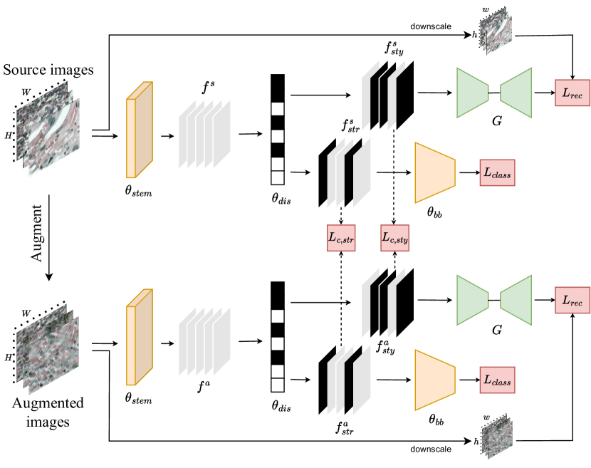
Figure 1: Overview of the proposed method. The feature maps, that result from passing original and augmented images through the first convolutional layer $\theta_{stem}$ of the backbone are further disentangled in a channel-wise manner via the module $\theta_{dis}$ into structure- and style-related components. Structure-related features are passed further into classification backbone $\theta_{bb}$ and are used to compute classification loss, while style-related ones go through the reconstruction network $G$ for further computation of the reconstruction loss. Additionally contrastive loss is used to minimize the distance between the structure-related components and maximize it between the style-related ones with the dotted lines representing a learnable projection into a lower dimension feature space.

In order to overcome the challenges that the classification task in SDG setting poses, we propose the reconstruction-based style regularization in conjunction with the technique of channel-wise contrastive disentanglement. Given the source domain data $\mathcal{D}^{s}=\left\{x_{i}^{s},y_{i}^{s}\right\}_{i=1}^{N_{s}}$, where $x_{i}^{s}\in\mathbb{R}^{C\times W\times H}$ is an image and $y_{i}^{s}\in\{0,1\}$ is a binary cancer presence label, we aim to train a model that will generalize well to a set of unseen target domains. The training process is outlined on the Figure 1.

2.0.1 Contrastive disentanglement.

First, in addition to the set of source images $x^{s}$ two sets of augmented images $x^{a}$ and $x^{b}$ are generated using two different strategies of data augmentations: Bezier curve transformation from SLAug [14] and low-frequency component replacement [20] (Figure 1 only shows $x^{a}$ for simplicity). All resulting sets of images pass through the first layer $\theta_{stem}$ of a classification backbone and the corresponding shallow-level feature maps $f^{s},f^{a}$ and $f^{b}$ are obtained. These feature maps are believed to carry significant style-related information [18] therefore we further perform the style/structure disentanglement by splitting the channels of each of them into two separate feature maps $f_{sty}$ and $f_{str}$, using a learnable parameter, denoted as $\theta_{dis}\in\mathbb{R}^{2\times 64}$:

$$f_{str},f_{sty}=f\times softmax(\theta_{dis}/\tau)$$ (1)

where $\tau$ is the temperature parameter and the $softmax$ is applied along the second dimension.

The contrastive loss components are computed following the idea that after disentanglement $f_{str}^{s},f_{str}^{a}$ and $f_{str}^{b}$ have to be the same as they represent the same structural pattern; while $f_{sty}^{s},f_{sty}^{a}$ and $f_{sty}^{b}$ have to be different due to style alteration caused by augmentations:

$$L_{c,str}=\frac{1}{2}\cdot\sum_{\begin{subarray}{c}i,j\in\{s,a,b\}\\ i\neq j\end{subarray}}|Proj(f_{str}^{i})-Proj(f_{str}^{j})|$$ (2)

$$L_{c,sty}=-\frac{1}{2}\cdot\sum_{\begin{subarray}{c}i,j\in\{s,a,b\}\\ i\neq j\end{subarray}}|Proj(f_{sty}^{i})-Proj(f_{sty}^{j})|$$ (3)

where the $Proj(\cdot)$ is a learnable operator, performing projection of the feature maps into a latent space of smaller dimension. On the Figure 1 it is represented by the dotted lines.

2.0.2 Style Regularization.

The next step involves computation of the style regularization loss components, which have been specifically designed to impose additional constraints on the style-dependent features $f_{sty}^{s},f_{sty}^{a}$ and $f_{sty}^{b}$ and improve the overall disentanglement capability of the architecture. To serve as the ground truth for the reconstruction, we utilize a downscaled version of the original images, which are believed to retain only style-related information due to resizing and the loss of their inherent structural features:

$$L_{rec}=\sum_{i\in\{s,a,b\}}\|G(f_{sty}^{i})-rs(x^{i})\|^{2},$$ (4)

where $G$ is the reconstruction network, and $rs$ is the resizing operator.

2.0.3 Classification backbone.

All of the structure-related feature maps $f_{str}^{s},f_{str}^{a}$ and $f_{str}^{b}$ pass through the rest of the classification network $\theta_{bb}$ for further calculation of the binary cross-entropy classification loss.

3 Experimental Setup

3.0.1 Datasets.

The experiments are conducted using the binary classification dataset Camelyon17-WILDS, which is a patchified version of the original Camelyon17 [1] breast cancer whole-slide images dataset. The data was collected from five medical centers each representing a separate domain. All input images are sized $96\times 96$, and the labels indicate whether the central $32\times 32$ area contains any tumor tissue.

As depicted in Figure 2, sample images from the dataset showcase significant variations in texture throughout the different domains, making it a challenging task to develop a generalizable model.

(a) Center 0	(b) Center 1	(c) Center 2	(d) Center 3	(e) Center 4

Figure 2: Sample images from the domains of the five centers.

3.0.2 Evaluation Methods.

We use the DomainBed [3] evaluation protocol with training-domain validation model selection strategy. In order to properly estimate the generalization ability of the models in the SDG setting, we iteratively repeat training with each of the centers being set as the source domain while the union of the remaining four serve as the target domain.

3.0.3 Implementation Details.

The experiments were run on 24GB Quadro RTX 6000 GPU. All the models utilize ResNet18 [4] pre-trained on ImageNet [2] as a backbone. Each experiment was run for 50 epochs with the batch size of 256 using Adam optimizer [6] with the learning rate of $1e-3$. The temperature parameter $\tau$ was fixed at 0.1 similar to [5].

We apply the same data augmentation strategy that we use in our method to all the other methods for a fair comparison. By doing so we eliminate the possibility of data augmentations being the deciding factor in the model’s performance and equalize the total number images each model is fed during training. We additionally evaluate the empirical risk minimization (ERM) method without these augmentations for representativeness.

3.0.4 Ablation studies.

We conduct a study to investigate the impact of target resolution on the reconstructed image, thereby exploring the effects of varying downsampling factors on the original image. We hypothesize that a higher downsampling factor will result in the loss of firstly structure-related information from the original image and therefore stronger style dependency of the feature map utilized for reconstruction. However, we also acknowledge the possibility of a threshold beyond which excessively high downsampling factors may lead to the loss of crucial style-related information. In this work we check the reconstruction resolutions 96, 48 and 24.

We also study the impact of combining our method with various feature-map style-augmentation techniques. In the scope of this work we evaluate such methods as MixStyle [24], Domain Shift with Uncertainty (DSU) [9] and Correlated Style Uncertainty (CSU) [22].

Table 1: Results of the classification task using different algorithms. i-th medical center is denoted as $C_{i}$. Each value represents accuracy (%) averaged over three runs of training on the respective domain and evaluation on the unification of the rest. The standard deviation over seeds is given in the subscript. The best accuracy is highlighted in bold and the second best accuracy underscored.

	$C_{0}$	$C_{1}$	$C_{2}$	$C_{3}$	$C_{4}$	Average
Vanilla ERM	$83.1_{\pm 0.9}$	$65.2_{\pm 1.1}$	$58.0_{\pm 0.4}$	$64.8_{\pm 1.9}$	$56.2_{\pm 0.8}$	$65.4$
ERM	$87.0_{\pm 0.7}$	$81.0_{\pm 2.2}$	$89.3_{\pm 0.4}$	$74.1_{\pm 1.5}$	$88.8_{\pm 0.5}$	$84.1$
$\text{C}^{2}\text{SDG}$	$\mathbf{90.2_{\pm 1.3}}$	$77.2_{\pm 1.0}$	$\mathbf{90.5_{\pm 0.3}}$	$72.5_{\pm 2.8}$	$89.4_{\pm 0.3}$	$83.9$
ConDiSR	$87.4_{\pm 0.6}$	$\mathbf{81.8_{\pm 1.0}}$	$90.4_{\pm 0.7}$	$\mathbf{75.0_{\pm 0.8}}$	$\mathbf{89.7_{\pm 0.6}}$	$\mathbf{84.9}$

4 Results and Discussion

Table 1 compares performance of our method versus ERM, $\text{C}^{2}$SDG [5] and ERM without augmentations (Vanilla ERM) in SDG setting for each separate center being set as the source domain. Each value is achieved by averaging three experimental results with different seeds.

As it can be seen from the Table 1, our method consistently outperforms baselines by the margin of $\sim 1\%$ as well as shows more stable performance with less deviation across the runs. We argue that reconstruction-based regularization aids the disentanglement module of the framework by enforcing stronger dependency between the input images and style-dependent channels of the shallow-level feature map. Due to direct interconnection this improves extraction of the structure-related channels as well.

The qualitative comparison of performance between $\text{C}^{2}\text{SDG}$ and ConDiSR on the Figure 3 shows that our method pays more attention to areas, containing semantically important information, which allows us to claim that the style regularization does indeed improve extraction of structural features as well.

The comparison between Vanilla ERM, ERM and $\text{C}^{2}\text{SDG}$ shows that the latter two mehtods achieve a significantly better performance than Vanilla ERM. However, when compared to each other, ERM and $\text{C}^{2}\text{SDG}$ have almost the same average accuracy, which leads us to believe that when it comes to the binary classification task, the primary driver of performance improvement of $\text{C}^{2}\text{SDG}$ might be extensive augmentations as well as increased number of training iterations resulting from the augmentation strategy in [5] rather than the idea of channel-wise contrastive disentanglement in its default version.

Table 2: Evaluation of the effect of changing the reconstruction resolution in ConDiSR. Standard deviation over three seeds is given in the subscript. The best accuracy (%) is highlighted in bold.

	$C_{0}$	$C_{1}$	$C_{2}$	$C_{3}$	$C_{4}$	Average
96 $\times$ 96	$86.8_{\pm 0.9}$	$\mathbf{83.0_{\pm 0.8}}$	$88.9_{\pm 1.1}$	$73.4_{\pm 0.4}$	$88.6_{\pm 0.5}$	$84.1$
48 $\times$ 48	$\mathbf{87.4_{\pm 0.6}}$	$81.8_{\pm 1.0}$	$\mathbf{90.4_{\pm 0.7}}$	$\mathbf{75.0_{\pm 0.8}}$	$\mathbf{89.7_{\pm 0.6}}$	$\mathbf{84.9}$
24 $\times$ 24	$83.4_{\pm 0.7}$	$81.3_{\pm 0.3}$	$89.1_{\pm 0.3}$	$73.1_{\pm 0.3}$	$87.5_{\pm 1.5}$	$82.9$

Table 3: Investigation of the effect of combining various style augmentation techniques with ConDiSR. Standard deviation over three seeds is given in the subscript. The best accuracy (%) is highlighted in bold.

	$C_{0}$	$C_{1}$	$C_{2}$	$C_{3}$	$C_{4}$	Average
MixStyle	$85.2_{\pm 0.4}$	$80.9_{\pm 0.8}$	$\mathbf{92.1_{\pm 0.1}}$	$73.7_{\pm 0.5}$	$\mathbf{91.1_{\pm 0.3}}$	$84.6$
+ ConDiSR	$\mathbf{87.2_{\pm 0.1}}$	$\mathbf{82.8_{\pm 0.5}}$	$\mathbf{92.1_{\pm 0.6}}$	$\mathbf{75.6_{\pm 0.6}}$	$90.6_{\pm 0.5}$	$\mathbf{85.7}$
DSU	$\mathbf{85.0_{\pm 0.7}}$	$81.4_{\pm 0.8}$	$\mathbf{91.1_{\pm 0.2}}$	$\mathbf{76.4_{\pm 1.0}}$	$\mathbf{90.2_{\pm 0.7}}$	$84.8$
+ ConDiSR	$84.5_{\pm 0.7}$	$\mathbf{84.2_{\pm 0.7}}$	$90.7_{\pm 0.4}$	$75.8_{\pm 0.8}$	$89.5_{\pm 0.6}$	$\mathbf{84.9}$
CSU	$\mathbf{86.0_{\pm 0.5}}$	$79.6_{\pm 2.1}$	$90.7_{\pm 0.2}$	$76.4_{\pm 0.6}$	$\mathbf{90.4_{\pm 0.4}}$	$84.6$
+ ConDiSR	$\mathbf{86.0_{\pm 0.4}}$	$\mathbf{85.7_{\pm 0.5}}$	$\mathbf{90.8_{\pm 0.7}}$	$\mathbf{78.1_{\pm 0.6}}$	$87.7_{\pm 0.9}$	$\mathbf{85.7}$

4.0.1 Reconstruction resolution.

From the Table 2 we can see that the optimal reconstruction resolution for our method is 48, which supports our preliminary assumption, that while performing the reconstruction-based style regularization, lack of any downsampling makes the style-related feature maps learn unnecessary structural features and hampers the work of disentanglement module. Conversely, if the target resolution is too low, the downsampling removes too much information from the source image, thereby diminishing the effect of style regularization technique.

4.0.2 Style augmentation.

As it can be seen in the Table 3, application of various style-augmentation methods [24] to the feature maps after each of the first three layers of the network does not provide any significant improvement compared to the baselines. However in conjunction with ConDiSR, it results in the highest accuracy reached, which raises an assumption that despite the usage of the disentanglement technique, structure-related feature maps extracted by our method still carry various important style-dependent features that are correlated with the classification label and benefit from augmentations.

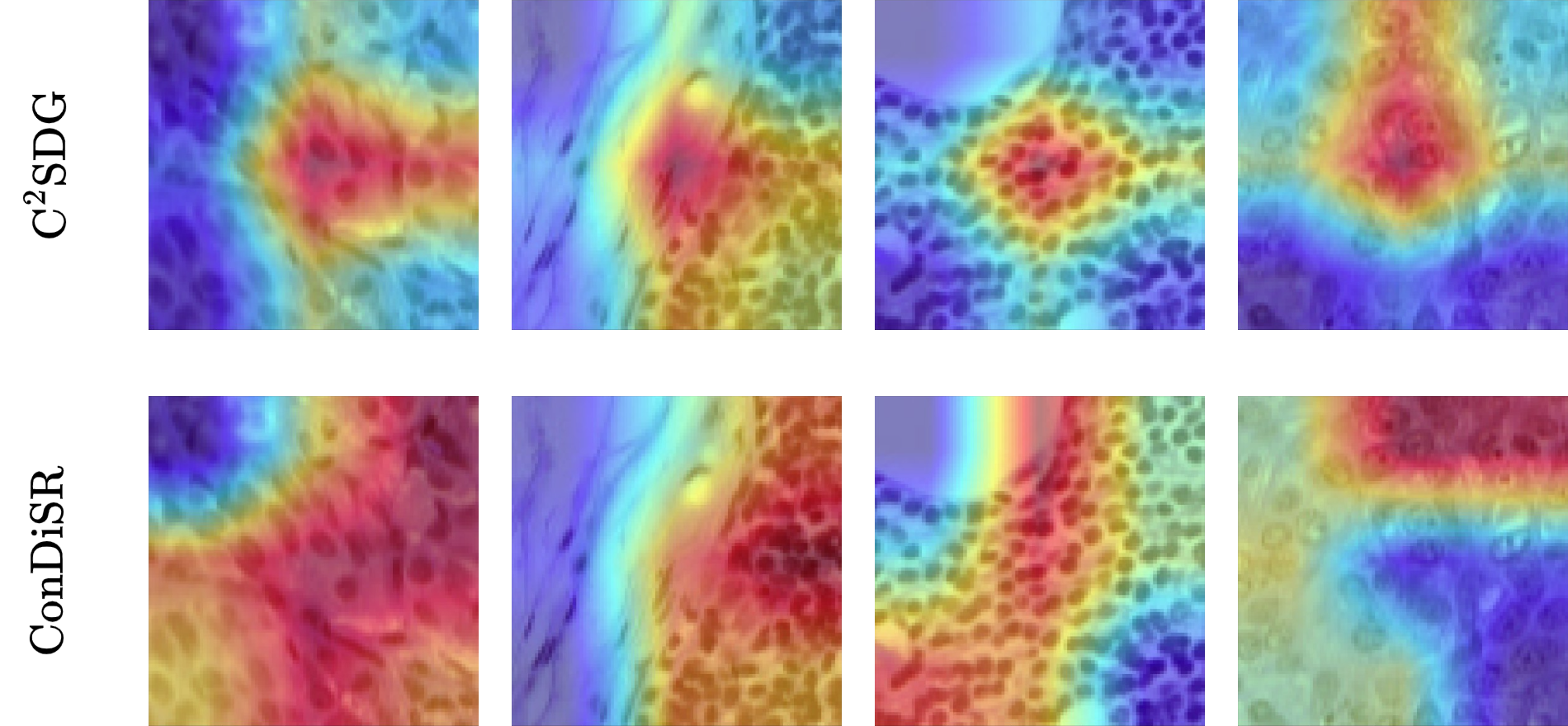
Figure 3: Qualitative performance comparison between ConDiSR and C²SDG [5] via Grad-CAM [12]

5 Conclusion

This paper presents a novel method, ConDiSR, designed for single domain generalization in the classification of images. Leveraging contrastive channel-wise disentanglement alongside style regularization through low-resolution reconstruction, ConDiSR demonstrates an improvement over baseline methods, achieving an increase in accuracy of approximately 1%. Successful application of ConDiSR shows the potential of disentanglement-based methodologies in enhancing model performance and generalizability, particularly in classification tasks within complex and heterogeneous datasets such as histopathology images. Our results underscore the importance of further exploration of disentanglement-based approaches and encourage further research in this domain. Potential future work may involve evaluation of the proposed method’s performance on other classification datasets in order to test its generalizability.

References

- [1] Bandi, P., Geessink, O., Manson, Q., Van Dijk, M., Balkenhol, M., Hermsen, M., Bejnordi, B.E., Lee, B., Paeng, K., Zhong, A., et al.: From detection of individual metastases to classification of lymph node status at the patient level: the camelyon17 challenge. IEEE Transactions on Medical Imaging (2018)
- [2] Deng, J., Dong, W., Socher, R., Li, L.J., Li, K., Fei-Fei, L.: Imagenet: A large-scale hierarchical image database. In: 2009 IEEE conference on computer vision and pattern recognition. pp. 248–255. Ieee (2009)
- [3] Gulrajani, I., Lopez-Paz, D.: In search of lost domain generalization (2020). https://doi.org/10.48550/ARXIV.2007.01434, https://arxiv.org/abs/2007.01434
- [4] He, K., Zhang, X., Ren, S., Sun, J.: Deep residual learning for image recognition. In: Proceedings of the IEEE conference on computer vision and pattern recognition. pp. 770–778 (2016)
- [5] Hu, S., Liao, Z., Xia, Y.: Devil is in channels: Contrastive single domain generalization for medical image segmentation. arXiv preprint arXiv:2306.05254 (2023)
- [6] Kingma, D.P., Ba, J.: Adam: A method for stochastic optimization. arXiv preprint arXiv:1412.6980 (2014)
- [7] Kouw, W.M., Loog, M.: An introduction to domain adaptation and transfer learning (2019)
- [8] Li, H., Wang, Y., Wan, R., Wang, S., Li, T.Q., Kot, A.: Domain generalization for medical imaging classification with linear-dependency regularization. Advances in neural information processing systems 33, 3118–3129 (2020)
- [9] Li, X., Dai, Y., Ge, Y., Liu, J., Shan, Y., Duan, L.Y.: Uncertainty modeling for out-of-distribution generalization. arXiv preprint arXiv:2202.03958 (2022)
- [10] Ouyang, C., Chen, C., Li, S., Li, Z., Qin, C., Bai, W., Rueckert, D.: Causality-inspired single-source domain generalization for medical image segmentation. IEEE Transactions on Medical Imaging 42(4), 1095–1106 (2022)
- [11] Qiao, F., Zhao, L., Peng, X.: Learning to learn single domain generalization. In: Proceedings of the IEEE/CVF Conference on Computer Vision and Pattern Recognition. pp. 12556–12565 (2020)
- [12] Selvaraju, R.R., Cogswell, M., Das, A., Vedantam, R., Parikh, D., Batra, D.: Grad-cam: Visual explanations from deep networks via gradient-based localization. International Journal of Computer Vision 128(2), 336–359 (Oct 2019). https://doi.org/10.1007/s11263-019-01228-7, http://dx.doi.org/10.1007/s11263-019-01228-7
- [13] Su, Z., Yao, K., Yang, X., Huang, K., Wang, Q., Sun, J.: Rethinking data augmentation for single-source domain generalization in medical image segmentation. In: Proceedings of the AAAI Conference on Artificial Intelligence. vol. 37, pp. 2366–2374 (2023)
- [14] Su, Z., Yao, K., Yang, X., Wang, Q., Sun, J., Huang, K.: Rethinking data augmentation for single-source domain generalization in medical image segmentation (2022)
- [15] Varoquaux, G., Cheplygina, V.: Machine learning for medical imaging: methodological failures and recommendations for the future. NPJ digital medicine 5(1), 48 (2022)
- [16] Wang, J., Du, R., Chang, D., Liang, K., Ma, Z.: Domain generalization via frequency-domain-based feature disentanglement and interaction. In: Proceedings of the 30th ACM International Conference on Multimedia. MM ’22, ACM (Oct 2022). https://doi.org/10.1145/3503161.3548267, http://dx.doi.org/10.1145/3503161.3548267
- [17] Wilson, G., Cook, D.J.: A survey of unsupervised deep domain adaptation. ACM Transactions on Intelligent Systems and Technology (TIST) 11(5), 1–46 (2020)
- [18] Xie, X., Niu, J., Liu, X., Chen, Z., Tang, S., Yu, S.: A survey on incorporating domain knowledge into deep learning for medical image analysis. Medical Image Analysis 69, 101985 (Apr 2021). https://doi.org/10.1016/j.media.2021.101985, http://dx.doi.org/10.1016/j.media.2021.101985
- [19] Xu, C., Wen, Z., Liu, Z., Ye, C.: Improved domain generalization for cell detection in histopathology images via test-time stain augmentation. In: International Conference on Medical Image Computing and Computer-Assisted Intervention. pp. 150–159. Springer (2022)
- [20] Yang, Y., Soatto, S.: Fda: Fourier domain adaptation for semantic segmentation (2020)
- [21] Zhang, Y., Wei, Y., Wu, Q., Zhao, P., Niu, S., Huang, J., Tan, M.: Collaborative unsupervised domain adaptation for medical image diagnosis. IEEE Transactions on Image Processing 29, 7834–7844 (2020)
- [22] Zhang, Z., Wang, B., Jha, D., Demir, U., Bagci, U.: Domain generalization with correlated style uncertainty. In: Proceedings of the IEEE/CVF Winter Conference on Applications of Computer Vision. pp. 2000–2009 (2024)
- [23] Zhou, K., Liu, Z., Qiao, Y., Xiang, T., Loy, C.C.: Domain generalization: A survey. IEEE Transactions on Pattern Analysis and Machine Intelligence pp. 1–20 (2022). https://doi.org/10.1109/tpami.2022.3195549, https://doi.org/10.1109%2Ftpami.2022.3195549
- [24] Zhou, K., Yang, Y., Qiao, Y., Xiang, T.: Domain generalization with mixstyle (2021)