Exploring the lepton flavor violating decay modes $b\to s\mu^{\pm}\tau^{\mp}$ in SMEFT approach

Abstract

We perform an analysis of the consequences of various new physics operators on the lepton flavor violating (LFV) decay modes mediated through $b\to s\ell_{1}\ell_{2}$ transitions. We scrutinize the imprints of the (pseudo)scalar and axial(vector) operators on the exclusive LFV decay channels $B_{(s)}\rightarrow(\phi,K^{*},K_{2}^{*})\ell_{1}\ell_{2}$ and $\Lambda_{b}\rightarrow\Lambda\ell_{1}\ell_{2}$, where $\ell_{1},\ell_{2}$ represent $\mu$ or $\tau$. The new physics parameters are constrained by using the upper limits of the branching fractions of the $B\to\tau\mu$ and $B\to K\tau\mu$ processes, assuming the new physics couplings to be real. We then explore the key observables such as the branching fraction, the forward-backward asymmetry, and the longitudinal polarisation fraction of the $B\to(K^{*},\phi,K_{2}^{*})\tau^{\pm}\mu^{\mp}$ decays. In addition, we also investigate the impact of the new physics couplings on the baryonic $\Lambda_{b}\to\Lambda\tau^{\pm}\mu^{\mp}$ decay channels mediated by the $b\to s$ quark level transition. With the experimental prospects at LHCb upgrade and Belle II, we also predict the upper limits of the above-discussed observables, which could intrigue the new physics search in these channels.

I Introduction

The Standard Model (SM) addresses elementary particles and their interactions, providing a comprehensive framework that firmly establishes a wide range of natural phenomena occurring at energies below the electroweak scale. Despite its remarkable achievements, the pursuit of physics beyond the Standard Model (BSM) remains crucial. This quest addresses numerous experimental anomalies and theoretical puzzles, including the prevalence of matter over antimatter in the universe, the enigma of dark matter and dark energy, as well as the hierarchy and flavor problems, among others. The potential existence of physics beyond the Standard Model arises from two distinct avenues. The first involves indirect effects of new physics (NP) associated with the presence of heavy new particles, which can modify the Wilson coefficients of the interaction Hamiltonian within the Standard Model framework. Alternatively, direct approaches entail detecting new particles through ongoing and upcoming collider experiments. Among various searches for physics beyond the SM, the $B$ meson decays have been considered as one of the potential avenues for BSM search in the indirect approach for many years. In this respect, the flavor-changing neutral current transition (FCNC) mediated decays, especially the $(b\to s/d)$ transitions are more captivating for understanding the nature of rare $b$ quark decays. The LHC at CERN, particularly LHCb LHCb:2022qnv ; LHCb:2022vje collaboration recently confirmed the lepton flavor universality (LFU) violating ratio $R_{K^{(*)}}=\mathcal{B}(B\to K^{(*)}\mu\mu)/\mathcal{B}(B\to K^{(*)}ee)$ to be consistent with the SM, which are of the order of unity. On the other hand, there exist various other observables such as the form factor independent (FFI) observable $P_{5}^{\prime}$ in $B\to K^{*}\mu^{-}\mu^{+}$ process and the branching ratios of several decay channels display few sigma deviations from the SM values. The LHCb LHCb:2013ghj ; LHCb:2015svh and ATLAS ATLAS:2018gqc collaborations reported a 3.3$\sigma$ difference from the SM prediction in the measurement of the celebrated $P_{5}^{\prime}$ observable. The other LFU violating observables, respecting the $b\to s$ quark level transitions, $R_{K_{S}^{0}}$ and $R_{K^{*+}}$ LHCb:2021lvy also show deviations at the level of $1.4\sigma$ and $1.5\sigma$ compared to the SM predictions, respectively. On the other hand, the branching fraction of the rare $B_{s}\to\phi\mu\mu$ decay mode reveals $3.3\sigma$ LHCb:2021zwz away from the SM value in $q^{2}\in[1.1,6.0]\leavevmode\nobreak\ \rm GeV^{2}$.

Unlike the lepton flavor-conserving decays, the LFV transitions indicate a clean probe of NP as they are forbidden in the SM. Various LFV decays in the charged lepton sector i.e., $\ell_{i}\to\ell_{j}\gamma$, $\ell_{i}\to\ell_{j}\ell_{k}\bar{\ell}_{k}$ as well as in $B$ meson sector, mediated through $b\to s\ell_{i}\ell_{j}$ transitions, have been extensively studied in the literature Lee:2015qra ; Altmannshofer:2015mqa ; Crivellin:2015mga ; Alonso:2015sja ; Sahoo:2015pzk ; Sahoo:2015wya ; Mohapatra:2023hhf ; Ali:2023kua . The LFV $B$ meson decays provide an ideal platform for NP search, particularly the results from LHCb and Belle II experiments can be used as a guiding principle in this direction. However, so far we have only the experimental upper limits for these decay modes. The LHCb experiment reported the upper bound on the branching ratio of the purely leptonic $B_{s}\to e^{\pm}\mu^{\mp}$ decay channel, which is found to be $\mathcal{B}(B_{s}\to e^{\pm}\mu^{\mp})<6.3\times 10^{-9}$ at 90% C.L. In addition, an upper limit of $4.2\times 10^{-5}$ in the branching fraction of $B\to\tau\mu$ has also been reported by the LHCb experiment LHCb:2019ujz . The LFV searches in semileptonic $B$ decays, on the other hand, include well-known decays like $B\to K\ell_{1}\ell_{2}$ processes, where $\ell_{1}$ or $\ell_{2}=e,\mu,\tau$. Based on Run I data with integrated luminosity 9 ${\rm fb}^{-1}$, an exclusion limit on $\mathcal{B}(B\to K\mu^{-}e^{+})<7\times 10^{-9}$ is reported by LHCb collaboration LHCb:2019bix . Similar searches were also performed for $B\to V\ell_{1}\ell_{2}$ ($V=K^{*},\phi$) processes. The current limit on the branching ratios of $B\to K^{*}\mu e$ and $B\to\phi\mu e$, set by LHCb, are $6.8\times 10^{-9}$ and $10.1\times 10^{-9}$, respectively. Despite the experimental difficulties due to missing energy during reconstruction from the environment of $\tau$ lepton present in the final state of the $B$ meson decays, Belle Belle:2022pcr experiment put an upper limit on the branching ratio of $B^{+}\to K^{+}\mu^{\pm}\tau^{\mp}$ decay mode as $3.9\times 10^{-5}$. An analysis is performed using the LHCb data LHCb:2022wrs on the $B\to K^{*}\mu^{\pm}\tau^{\mp}$ process. However, no signal is observed, instead, an upper limit on the branching fraction of $B\to K^{*}\tau^{+}\mu^{-}$ and $B\to K^{*}\tau^{-}\mu^{+}$ are set to be $1.0\times 10^{-5}$ and $8.2\times 10^{-6}$ LHCb:2022wrs at the 90$\%$ confidence level.

In this work, we would like to explore the effect of the SMEFT (Standard Model Effective Field Theory) formalism on the exclusive semileptonic $b\to s\tau\mu$ decays. Given the current and future experimental prospects, we mainly focus on the $B\to(K^{*},\phi,K_{2}^{*})\tau^{\pm}\mu^{\mp}$ decays. In addition, we also investigate the impact of the new physics couplings on the baryonic $\Lambda_{b}\to\Lambda\tau^{\pm}\mu^{\mp}$ decay channels mediated by $b\to s$ quark level transition. Our fit anatomy includes the upper limit of the branching ratios of the leptonic $B\to\tau\mu$ and semileptonic $B\to K\tau\mu$ processes. Using the constrained values of the NP couplings, we probe the prominent observables such as the branching fraction, the forward-backward asymmetry, and the longitudinal polarisation fraction of the above decay modes in the presence of various SMEFT operators.

The paper is organized in the following manner. In section II, we recapitulate the theoretical framework of the EFT framework of $b\rightarrow s\ell_{1}\ell_{2}$ transition. We also discuss on various observable associated with the $B_{(s)}\to(K^{*},\phi,K_{2}^{*})\ell_{1}\ell_{2}$ and $\Lambda_{b}\to\Lambda\ell_{1}\ell_{2}$ processes. In section III, we constrain the new physics parameter space in the presence of various SMEFT operators. We interpret the outcome followed by numerical analysis of the $B\to(K^{*},\phi,K_{2}^{*})\tau^{\pm}\mu^{\mp}$ and the baryonic $\Lambda_{b}\to\Lambda\tau^{\pm}\mu^{\mp}$ decays in the presence of new physics coefficients. Finally, we conclude our work in section IV.

II Theoretical Framework

The most generic effective Hamiltonian describing the $b\to s\ell_{1}^{-}\ell_{2}^{+}$ decay is given as Das:2019omf

$$\begin{split}\mathcal{H}_{eff}=-\frac{4G_{F}}{\sqrt{2}}V_{tb}V^{*}_{ts}\frac{\alpha_{em}}{4\pi}\sum_{i=9,10,S,P}\big{(}C_{i}^{\ell_{1}\ell_{2}}(\mu)\mathcal{O}_{i}^{\ell_{1}\ell_{2}}(\mu)+C_{i}^{{}^{\prime}\ell_{1}\ell_{2}}(\mu)\mathcal{O^{\prime}}_{i}^{\ell_{1}\ell_{2}}(\mu)\big{)},\end{split}$$ (1)

where $G_{F}$ and $V_{tb}V_{ts}^{*}$ are the Fermi coupling constant and CKM matrix elements respectively. The relevant operators for the process are expressed as follows,

$$\begin{split}&\mathcal{O}^{(\prime)}_{9}=\big{[}\bar{s}\gamma^{\mu}P_{L(R)}b\big{]}\big{[}\ell_{2}\gamma_{\mu}\ell_{1}\big{]}\,,\quad\mathcal{O}^{(\prime)}_{10}=\big{[}\bar{s}\gamma^{\mu}P_{L(R)}b\big{]}\big{[}\ell_{2}\gamma_{\mu}\gamma_{5}\ell_{1}\big{]}\;,\\ &\mathcal{O}_{S}^{(\prime)}=\big{[}\bar{s}P_{R(L)}b\big{]}\big{[}\ell_{2}\ell_{1}\big{]}\,,\quad\quad\quad\mathcal{O}_{P}^{(\prime)}=\big{[}\bar{s}P_{R(L)}b\big{]}\big{[}\ell_{2}\gamma_{5}\ell_{1}\big{]}\,.\end{split}$$ (2)

Here, the operators $\mathcal{O}_{9,10,S,P}$ represent the vector, axial-vector, scalar, and pseudoscalar operators, respectively. The primed operators $\mathcal{O}_{i}^{\prime}$ can be obtained by flipping the chirality of the former operators $\mathcal{O}_{i}$. The $C^{(\prime)}_{9,10,S,P}$ are the Wilson coefficients that have zero value in the SM and can have a non-zero value in various new physics scenarios. In SM, the leptons $\ell_{1},\ell_{2}$ correspond to the same flavor which is usually considered as $\ell$.

The decay observables of $b\to s\ell_{1}\ell_{2}$ transitions

II.0.1 Exclusive $\Lambda_{b}\rightarrow\Lambda\ell_{1}\ell_{2}$ decay channel

To illustrate the kinematics of the $\Lambda_{b}\rightarrow\Lambda\ell_{1}\ell_{2}$ decay mode, we assume the baryon $\Lambda_{b}$ is at rest, while the final state particles $\Lambda$ and the dilepton pair travel along the positive and negative $z$-axis, respectively. The momenta assigned to the particles $\Lambda_{b}$, $\Lambda$, $\ell_{1}$, and $\ell_{2}$ are represented by the symbols $p$, $k$, $q_{1}$, and $q_{2}$ respectively. The spin of the baryon $\Lambda_{b}$ ($\Lambda$) on to the z-axis in the rest frame is denoted as $s_{p}(s_{k})$. The decay amplitude of the exclusive $\Lambda_{b}\rightarrow\Lambda\ell_{1}\ell_{2}$ process can be written as Das:2019omf ,

$$\begin{split}\mathcal{M}^{\lambda_{1},\lambda_{2}}(s_{p},s_{k})=-\frac{V_{tb}V_{ts}^{*}}{2v^{2}}\frac{\alpha_{em}}{4\pi}\sum_{i=L,R}\Big{[}\sum_{\lambda}\eta_{\lambda}H_{VA,\lambda}^{i,s_{p},s_{k}}L_{i,\lambda}^{\lambda_{2},\lambda_{1}}+H_{SP}^{i,s_{p},s_{k}}L_{i}^{\lambda_{2},\lambda_{1}}\Big{]}.\end{split}$$ (3)

In the dilepton rest frame, $q^{\mu}$ represents the four-momentum of the dilepton pair, and $\theta_{\ell}$ denotes the angle between the $\ell_{1}$ and $z$-axis of the dilepton rest frame. Here the hadronic helicity amplitude $H_{VA(SP),\lambda}^{i,s_{p},s_{k}}$ correspond to the vector-axial vector (scalar-pseudoscalar) operators whereas the $L_{i,\lambda}^{\lambda_{2},\lambda_{1}}$, and $L_{i}^{\lambda_{2},\lambda_{1}}$ are the leptonic helicity amplitudes.

For the detailed expression of the lepton helicity amplitude, we refer to Ref. Das:2019omf . Here $i=L,R$ correspond to the chiralities of the lepton current, and $\lambda=t,\pm 1,0$ represents the helicity state of the virtual gauge boson that decays into the dilepton pair. The symbols $\lambda_{1,2}$ are the helicities of the leptons. Additionally, the parameters $\eta_{t}$ and $\eta_{\pm 1,0}$ are assigned a value of 1 and -1, respectively. The expressions of $H_{VA,\lambda}^{i,s_{p},s_{k}}$ and $H_{SP,\lambda}^{i,s_{p},s_{k}}$ in terms of Wilson coefficients (WCs) and form factors (FFs) can be found in Das:2018sms . Alternatively, in the literature, transversity amplitudes: $A_{\perp(||)1}^{i},\leavevmode\nobreak\ A_{\perp(||)0}^{i}$ and $A_{S\perp(||)},\leavevmode\nobreak\ A_{P\perp(||)}$ are often employed instead of the hadronic helicity amplitudes. The expressions for these transversity amplitudes can be found in Ref. Das:2019omf . The amplitudes $L_{i,\lambda}^{\lambda_{2},\lambda_{1}}$ and $L_{i}^{\lambda_{2},\lambda_{1}}$ are defined as follows:

$$\begin{split}&L^{\lambda_{2},\lambda_{1}}_{L(R)}=\langle\bar{\ell}_{2}(\lambda_{2})\ell_{1}(\lambda_{1})|\bar{\ell}_{2}(1\mp\gamma_{5})\ell_{1}|0\rangle\,,\\ &L^{\lambda_{2},\lambda_{1}}_{L(R),\lambda}=\bar{\epsilon}^{\mu}(\lambda)\langle\bar{\ell}_{2}(\lambda_{2})\ell_{1}(\lambda_{1})|\bar{\ell}_{2}\gamma_{\mu}(1\mp\gamma_{5})\ell_{1}|0\rangle\,.\end{split}$$ (4)

Here, $\epsilon^{\mu}$ represents the polarization vector of the virtual gauge boson that decays into the dilepton pair. The detailed calculations of $L_{i,\lambda}^{\lambda_{2},\lambda_{1}}$ and $L_{i}^{\lambda_{2},\lambda_{1}}$ can be found in Ref. Das:2019omf . Based on these definitions, one can derive the differential branching ratio of $\Lambda_{b}\rightarrow\Lambda\ell_{1}\ell_{2}$ as follows:

$$\begin{split}\frac{d^{2}{\cal B}}{dq^{2}d\cos\theta_{l}}=\frac{3}{2}(K_{1ss}\sin^{2}\theta_{l}+K_{1cc}\cos^{2}\theta_{l}+K_{1c}\cos\theta_{l})\;.\end{split}$$ (5)

The angle $\theta_{\ell}$ can vary within the range $-\pi\leq\theta_{\ell}\leq\pi$. The long-distance aspect of the decay is encapsulated within the $\Lambda_{b}\rightarrow\Lambda$ transition matrix elements, which are parameterized in terms of six $q^{2}$-dependent form factors, denoted as $f_{t,0,\perp}^{V/A}$ Feldmann:2011xf . For our numerical analysis, we utilize the form factors obtained from lattice QCD calculations Detmold:2016pkz . The resulting differential branching ratio is given by:

$$\frac{d\mathcal{B}}{dq^{2}}=2K_{1ss}+K_{1cc}\,.$$ (6)

Additionally, the FBA (Forward-backward asymmetry) is expressed as,

$$A^{\ell}_{\rm FB}=\frac{3}{2}\frac{K_{1c}}{K_{1ss}+K_{1cc}}\,,$$ (7)

where the squared dilepton invariant mass ($q^{2}$) varies within the range $(m_{1}+m_{2})^{2}\leq q^{2}\leq(m_{\Lambda_{b}}-m_{\Lambda})^{2}$.

II.0.2 Exclusive $B\to K_{2}^{*}\ell_{1}\ell_{2}$ decay channel

Utilizing the effective Hamiltonian governing $b\to s\ell_{1}\ell_{2}$ transition, provided in Eq. (1), one can derive the transition amplitude for the $B\to K_{2}^{*}\ell_{1}\ell_{2}$ decay mode. The hadronic matrix elements of vector and axial-vector currents for $B\to K_{2}^{*}$ transitions can be parameterized in terms of $q^{2}$-dependent FFs: $V(q^{2})$ and $A_{0,1,2}(q^{2})$. The expressions in detail are given as follows Wang:2010ni ,

$$\langle K_{2}^{*}(k,\epsilon^{*})|\bar{s}\gamma^{\mu}b|\overline{B}(p)\rangle = -\frac{2V(q^{2})}{m_{B}+m_{K_{2}^{*}}}\epsilon^{\mu\nu\rho\sigma}\epsilon^{*}_{T\nu}p_{\rho}k_{\sigma},$$

$$\langle K_{2}^{*}(k,\epsilon^{*})|\bar{s}\gamma^{\mu}\gamma_{5}b|\overline{B}(p)\rangle = i(m_{B}+m_{K_{2}^{*}})A_{1}(q^{2})\left[\epsilon^{*\mu}_{T}-\frac{\epsilon^{*}_{T}\cdot q}{q^{2}}q^{\mu}\right]+2im_{K_{2}^{*}}A_{0}(q^{2})\frac{\epsilon^{*}_{T}\cdot q}{q^{2}}q^{\mu}$$ (8)

$$-iA_{2}(q^{2})\frac{\epsilon^{*}_{T}\cdot q}{m_{B}+m_{K_{2}^{*}}}\left[(p+k)^{\mu}-\frac{m_{B}^{2}-m_{K_{2}^{*}}^{2}}{q^{2}}q^{\mu}\right],$$

where, $p$ ($k$) is the four momentum of $B$ ($K_{2}^{*}$) meson.

We employ the recent values of form factors from the light cone QCD sum rule (LCSR) approach given in Ref. Aliev:2019ojc . In this method, the form factors can be expressed as

$$F^{B\to T}=\frac{1}{1-q^{2}/m_{R,F}^{2}}\sum_{n=0}^{1}\alpha_{n}^{F}[z(q^{2})-z(0)]^{n},$$ (9)

where $z(q^{2})=\frac{\sqrt{t_{+}-q^{2}}-\sqrt{t_{+}-t_{0}}}{\sqrt{t_{+}-q^{2}}+\sqrt{t_{+}-t_{0}}}$,   $t_{\pm}=(m_{B}{\pm}m_{K_{2}^{*}})^{2}$,   $t_{0}=t_{+}(1-\sqrt{1-t_{-}/t_{+}})$ and $m_{R,F}$ is the resonance mass corresponding to the form factor. The associated parameters are provided in Table 1. The resonance masses employed in our numerical calculations are given as

$$m_{R,A_{0}}=5.336\hskip 2.84544pt{\rm GeV},\hskip 14.22636ptm_{R,V}=5.412\hskip 2.84544pt{\rm GeV},\hskip 14.22636ptm_{R,(A_{1},A_{3})}=5.829\hskip 2.84544pt{\rm GeV}.$$ (10)

Form factor	$\alpha_{0}$	$\alpha_{1}$
$V^{B\to K_{2}^{*}}$	$0.22^{+0.11}_{-0.08}$	$-0.90^{+0.37}_{-0.50}$
$A^{B\to K_{2}^{*}}_{0}$	$0.30^{+0.01}_{-0.05}$	$-1.23^{+0.23}_{-0.23}$
$A^{B\to K_{2}^{*}}_{1}$	$0.19^{+0.09}_{-0.07}$	$-0.46^{+0.19}_{-0.25}$
$A^{B\to K_{2}^{*}}_{2}$	$0.11^{+0.05}_{-0.06}$	$-0.40^{+0.23}_{-0.16}$

Table 1: Fit parameters corresponding to $B\to K_{2}^{*}$ form factors in LCSR method

The differential decay distribution describing three body $B\to K_{2}^{*}\ell_{1}\ell_{2}$ decay can be expressed as Kumbhakar:2022szr

$$\frac{d^{2}\Gamma}{dq^{2}d\cos\theta_{\ell}}=A(q^{2})+B(q^{2})\cos\theta_{\ell}+C(q^{2})\cos^{2}\theta_{\ell}\;,$$ (11)

where $\theta_{\ell}$ is the leptonic polar angle which describes the angle made by lepton $\ell_{1}$ to the dilepton rest frame. The $q^{2}$-dependent coefficients $A(q^{2}),B(q^{2})$, and $C(q^{2})$ are given in Appendix -B. Using Eq. (11), the differential decay rate can be given as

$$\frac{d\Gamma}{dq^{2}}=2\left(A+\frac{C}{3}\right),$$ (12)

and the lepton FBA is found to be

$$A_{\rm FB}(q^{2})=\frac{1}{d\Gamma/dq^{2}}\left(\int_{0}^{1}d\cos\theta_{\ell}\frac{d^{2}\Gamma}{d\cos\theta_{\ell}dq^{2}}-\int_{-1}^{0}d\cos\theta_{\ell}\frac{d^{2}\Gamma}{d\cos\theta_{\ell}dq^{2}}\right)=\frac{B}{2\left(A+\frac{C}{3}\right)}\;.$$ (13)

II.0.3 Exclusive $B\rightarrow(K^{*},\phi)\ell_{1}^{-}\ell_{2}^{+}$ decay channel

For the analysis of the decay $B\rightarrow(K^{*},\phi)\ell_{1}^{-}\ell_{2}^{+}$, we adopt the kinematics and the angular conventions as described in references Korner:1989qb ; Becirevic:2016zri . The hadronic matrix elements involve a more extensive set of $q^{2}$-dependent form factors which include

$$\langle\bar{K}^{\ast}(k)|\bar{s}\sigma_{\mu\nu}q^{\nu}(1-\gamma_{5})b|\bar{B}(p)\rangle =2i\varepsilon_{\mu\nu\rho\sigma}\varepsilon^{\ast\nu}p^{\rho}k^{\sigma}T_{1}(q^{2})-[(\varepsilon^{\ast}\cdot q)(2p-q)_{\mu}-\varepsilon_{\mu}^{\ast}(m_{B}^{2}-m_{K^{\ast}}^{2})]T_{2}(q^{2})$$

$$-(\varepsilon^{\ast}\cdot q)\Big{[}\frac{q^{2}}{m_{B}^{2}-m_{K^{\ast}}^{2}}(p+k)_{\mu}-q_{\mu}\Big{]}T_{3}(q^{2}),$$

$$\langle\bar{K}^{\ast}(k)|\bar{s}\gamma^{\mu}(1-\gamma_{5})b|\bar{B}(p)\rangle =\varepsilon_{\mu\nu\rho\sigma}\varepsilon^{\ast\nu}p^{\rho}k^{\sigma}\frac{2V(q^{2})}{m_{B}+m_{K^{\ast}}}-i\Big{[}\varepsilon_{\mu}^{\ast}(m_{B}+m_{K^{\ast}})A_{1}(q^{2})$$

$$-i(p+k)_{\mu}(\varepsilon^{\ast}\cdot q)\frac{A_{2}(q^{2})}{m_{B}+m_{K^{\ast}}}-q_{\mu}(\varepsilon^{\ast}\cdot q)\frac{2m_{K^{\ast}}}{q^{2}}[A_{3}(q^{2})-A_{0}(q^{2})]\Big{]}.$$ (14)

The polarisation vector of the $K^{*}(\phi)$ meson is denoted as $\varepsilon_{\mu}$. The form factor $A_{3}(q^{2})$ related to $A_{1}(q^{2})$ and $A_{2}(q^{2})$ is given by $2m_{V}A_{3}(q^{2})=(m_{B}+m_{V})A_{1}(q^{2})-(m_{B}-m_{V})A_{2}(q^{2})$.

The $q^{2}$-dependent differential branching ratio, after integrating the full angular distribution over the angles given in Appendix C, is expressed as

$$\begin{split}\frac{d{\cal B}}{dq^{2}}=\frac{1}{4}[3I_{1}^{c}(q^{2})+6I_{1}^{s}(q^{2})-I_{2}^{c}(q^{2})-2I_{2}^{s}(q^{2})].\end{split}$$ (15)

The form factors associated with the transversity amplitude are obtained using the LCSR method Bharucha:2015bzk and are expressed as follows:

$$F_{i}(q^{2})=\frac{1}{1-q^{2}/m_{R,i}^{2}}\sum_{k}\alpha_{k}^{i}[z(q^{2})-z(0)]^{k},$$ (16)

where $z(q^{2})=\frac{\sqrt{t_{+}-q^{2}}-\sqrt{t_{+}-t_{0}}}{\sqrt{t_{+}-q^{2}}+\sqrt{t_{+}-t_{0}}}$,  $t_{\pm}=(m_{B}{\pm}m_{V})^{2}$,  $t_{0}=t_{+}(1-\sqrt{1-t_{-}/t_{+}})$ and $m_{R,F}$ is the resonance mass corresponding to the form factor. In our calculations, we use the resonance masses as follows:

$$m_{R,A_{0}}=5.336\hskip 2.84544pt{\rm GeV},\hskip 14.22636ptm_{R,(V,T_{1})}=5.412\hskip 2.84544pt{\rm GeV},\hskip 14.22636ptm_{R,(A_{1},A_{3},T_{2},T_{3})}=5.829\hskip 2.84544pt{\rm GeV}.$$ (17)

. We apply the above formalism originally developed for $B\to K^{*}$ decay to analyze the process $B\to\phi\ell_{1}\ell_{2}$. This is achieved by straightforwardly substituting the relevant mass and form factors for the corresponding vector meson $\phi$. The numerical values for the parameters associated with the form factors with $1\sigma$ uncertainty are given in Table 2.

$F_{i}$	$\alpha_{0}$	$\alpha_{1}$	$\alpha_{2}$
$V$	$0.34\pm 0.04$	$-1.05\pm 0.24$	$2.37\pm 1.39$
$A_{0}$	$0.36\pm 0.05$	$-1.04\pm 0.27$	$1.12\pm 1.35$
$A_{1}$	$0.27\pm 0.03$	$0.39\pm 0.19$	$-0.11\pm 0.48$
$A_{3}$	$0.26\pm 0.03$	$0.60\pm 0.20$	$0.12\pm 0.84$
$T_{1}$	$0.28\pm 0.03$	$-0.89\pm 0.19$	4$1.95\pm 1.10$
$T_{2}$	$0.28\pm 0.03$	$0.40\pm 0.18$	$0.36\pm 0.51$
$T_{3}$	$0.67\pm 0.08$	$1.48\pm 0.49$	$1.92\pm 1.96$

$F_{i}$	$\alpha_{0}$	$\alpha_{1}$	$\alpha_{2}$
$V$	$0.39\pm 0.03$	$-1.03\pm 0.25$	$3.50\pm 1.55$
$A_{0}$	$0.39\pm 0.05$	$-0.78\pm 0.26$	$2.41\pm 1.48$
$A_{1}$	$0.30\pm 0.03$	$0.48\pm 0.19$	$0.29\pm 0.65$
$A_{3}$	$0.25\pm 0.03$	$0.76\pm 0.20$	$0.71\pm 0.96$
$T_{1}$	$0.31\pm 0.03$	$-0.87\pm 0.19$	4$2.75\pm 1.19$
$T_{2}$	$0.31\pm 0.03$	$0.58\pm 0.19$	$0.89\pm 0.71$
$T_{3}$	$0.68\pm 0.07$	$2.11\pm 0.46$	$4.94\pm 2.25$

Table 2: Form factors for $B\to K^{*}\ell_{1}\ell_{2}$ (left panel) and $B_{s}\to\phi\ell_{1}\ell_{2}$ (right panel).

III phenomenological implication

SMEFT-inspired LFV transitions have garnered significant attention. Given the absence of any new particles observed thus far beyond the electroweak scale, it is conjectured that the scale of NP is substantially higher compared to the current running scale of the LHC. In this context, the SMEFT offers a powerful framework for elucidating LFV decays which encompasses a comprehensive set of dimension-six operators constructed from the fields of the Standard model. The corresponding Lagrangian is given as follows Grzadkowski:2010es :

$$\begin{split}\mathcal{L}_{SMEFT}&=\mathcal{L}_{SM}-\frac{1}{\Lambda_{\rm cut}^{2}}\Big{\{}[C^{(3)}_{lq}]^{ij\alpha\beta}(\bar{Q}^{i}\gamma^{\mu}\sigma^{a}Q^{j})(\bar{L}^{\alpha}\gamma_{\mu}\sigma^{a}L^{\beta})\\ &+[C^{(1)}_{lq}]^{ij\alpha\beta}(\bar{Q}^{i}\gamma^{\mu}Q^{j})(\bar{L}^{\alpha}\gamma_{\mu}L^{\beta})+[C_{ledq}^{ij\alpha\beta}(\bar{Q}^{i}d_{R}^{j})(\bar{e}_{R}^{\alpha}L^{\beta})]\Big{\}}.\end{split}$$ (18)

Here $Q$ and $L$ represent the left-handed quark and lepton fields, which transform as doublets under $SU(2)$ whereas $e_{R}$ and $d_{R}$ are the singlet right-handed charged leptons and down-type quarks, respectively. Here $\Lambda_{\rm cut}$ is the cut-off scale which can be associated with the mass of the heavy NP degrees of freedom. The above equation includes the set of all the dimension six operators contributing to the $b\to s\ell_{1}\ell_{2}$ transitions. It should be noted that none of these above operators contain tensor currents.

The SMEFT Wilson coefficients can be constrained from low energy processes, and are related to the Wilson coefficients in Eqn (1) as

$$C_{9}^{\ell_{1}\ell_{2}}=-C_{10}^{\ell_{1}\ell_{2}}=+\frac{v^{2}}{\Lambda_{\rm cut}^{2}}\frac{\pi}{\alpha_{em}|{V_{tb}V^{*}_{ts}}|}([C^{(3)}_{\ell q}]^{23\ell_{1}\ell_{2}}+[C^{(1)}_{\ell q}]^{23\ell_{1}\ell_{2}}),$$ (19)

$$C_{9}^{{}^{\prime}\ell_{1}\ell_{2}}=-{C^{\prime}}_{10}^{\ell_{1}\ell_{2}}=+\frac{v^{2}}{\Lambda_{\rm cut}^{2}}\frac{\pi}{\alpha_{em}{V_{tb}V^{*}_{ts}}|}([C_{\ell d}]^{23\ell_{1}\ell_{2}},$$ (20)

$$C_{S}^{\ell_{1}\ell_{2}}=-C_{P}^{\ell_{1}\ell_{2}}=+\frac{v^{2}}{\Lambda_{\rm cut}^{2}}\frac{\pi}{\alpha_{em}{V_{tb}V^{*}_{ts}}|}([C_{leqd}]^{23\ell_{1}\ell_{2}},$$ (21)

$$C_{S}^{{}^{\prime}\ell_{1}\ell_{2}}=-{C^{\prime}}_{P}^{\ell_{1}\ell_{2}}=+\frac{v^{2}}{\Lambda_{\rm cut}^{2}}\frac{\pi}{\alpha_{em}{V_{tb}V^{*}_{ts}}|}([C_{\ell eqd}^{*}]^{32\ell_{1}\ell_{2}}\;.$$ (22)

Now, we examine the constraints on various combinations of SMEFT Wilson coefficients derived from measurements of mesonic LFV decays. We consider the branching ratios of the decay modes $\bar{B}_{s}\rightarrow\ell_{1}^{-}\ell_{2}^{+}$ and $B\rightarrow K\ell_{1}^{-}\ell_{2}^{+}$ and use their experimental upper limits provided in Table 3 at 90$\%$ confidence level.

Observable	Exp.limit
$\mathcal{B}(B_{s}\to\mu^{\pm}\tau^{\mp})$	$4.2\times 10^{-5}$ LHCb:2019ujz
$\mathcal{B}(B^{+}\to K^{+}\mu^{-}\tau^{+})$	$3.9\times 10^{-5}$ LHCb:2020khb
$\mathcal{B}(B^{+}\to K^{+}\mu^{+}\tau^{-})$	$4.5\times 10^{-5}$ BaBar:2012azg

Table 3: Experimental upper limits for LFV $B$ decays at 90$\%$ C.L.

The branching fraction of these decay modes are expressed as Becirevic:2016oho ; Gratrex:2015hna

$$\mathcal{B}(\bar{B}_{s}\to\ell^{-}_{1}\ell^{+}_{2})= \,\frac{\tau_{B_{s}}}{64\pi^{3}}\frac{\alpha_{\text{em}}^{2}G_{F}^{2}|V_{tb}V_{ts}^{*}|^{2}}{m_{B_{s}}^{3}}f_{B_{s}}^{2}\,\lambda^{1/2}(m_{B_{s}}^{2},m_{\ell_{1}}^{2},m_{\ell_{2}}^{2})$$ (23)

$$\times \left\{[m_{B_{s}}^{2}-(m_{\ell_{1}}-m_{\ell_{2}})^{2}]\left|(m_{\ell_{1}}+m_{\ell_{2}}){C}_{10-}+\frac{m_{B_{s}}^{2}}{m_{b}+m_{s}}{C}_{P-}\right|^{2}\right.$$

$$+\left.[m_{B_{s}}^{2}-(m_{\ell_{1}}+m_{\ell_{2}})^{2}]\left|(m_{\ell_{1}}-m_{\ell_{2}})({C}_{9-})+\frac{m_{B_{s}}^{2}}{m_{b}+m_{s}}({C}_{S-})\right|^{2}\right\},$$

$$\mathcal{B}(B^{+}\to K^{+}\ell_{1}^{-}\ell_{2}^{+}) =10^{-8}\bigg{\{}c^{S}_{\ell_{1}\ell_{2}}\left|C_{S+}\right|^{2}+c^{P}_{\ell_{1}\ell_{2}}\left|C_{P+}\right|^{2}+c^{9+}_{\ell_{1}\ell_{2}}\left|C_{9+}\right|^{2}$$ (24)

$$+c^{10+}_{\ell_{1}\ell_{2}}\left|C_{10+}\right|^{2}+c^{S9}_{\ell_{1}\ell_{2}}\,\mathrm{Re}[C_{S+}^{*}C_{9+}]+c^{P10}_{\ell_{1}\ell_{2}}\,\mathrm{Re}[C_{P+}^{*}C_{10+}]\bigg{\}}\,,$$

where we have adopted the notation $C_{X\pm}=C_{X}\pm C_{X}^{\prime}$. To calculate the branching ratios for these processes, we use the values of particle masses from PDG ParticleDataGroup:2020ssz , CKM matrix elements from the UT-fit collaborations utfit , and the decay constant of $B_{s}$ meson as $f_{B_{s}}$=215 MeV Balasubramamian:2019wgx . The values of the coefficients $c^{i}_{\ell_{1}\ell_{2}}$ are taken from Bordone:2021usz . For our analysis, we utilize the Eqs. (23) and (24) to constrain the various combinations of SMEFT Wilson coefficients. For convenience, we sum over the oppositely charge lepton decays modes e.g., $\mathcal{B}(B_{s}\to\mu^{\pm}\tau^{\mp})=(B_{s}\to\mu^{-}\tau^{+})+(B_{s}\to\mu^{+}\tau^{-})$ and similarly for other channel as well. Here we consider the constraints coming from the $\mu\tau$ decay channel. It is generally established that consideration of primed operators is unappealing to fit the $b\to s\ell\ell$ data Alguero:2021anc ; Altmannshofer:2021qrr ; Hurth:2021nsi ; Ciuchini:2019usw ; Gratrex:2015hna and hence, the use of only unprimed operators is well accepted.

In Fig. 1, we illustrate the constrained parameter space governing the SMEFT Wilson coefficients for the final states involving $\tau\mu$. Here we focus on the two-dimensional scenario involving the SMEFT new physics couplings $[C^{(1)}_{\ell q}]^{23\ell_{1}\ell_{2}}$ and $[C_{leqd}]^{23\ell_{1}\ell_{2}}$ which enables us to elucidate the intricate relationship between these coefficients within the SMEFT framework.

IV Implications OF the Results

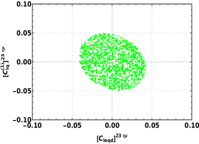
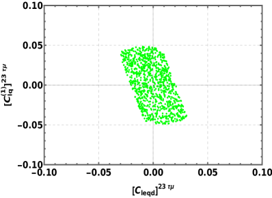
Figure 1: Constraints on the NP couplings obtained from the branching ratios of $B\to\tau\mu$ (top left) and $B\to K^{+}\tau\mu$ (top right). The lower panel illustrates for the combined measurement of ${\cal B}(B\to\tau\mu$) and ${\cal B}(B\to K^{+}\tau\mu$).

In this section, we illustrate the implications of our results in $b\to s\ell_{1}\ell_{2}$ transitions. The allowed parameter space is constrained by using the combined measurements of $B_{s}\to\tau^{\pm}\mu^{\mp}$ and $B\to K^{+}\tau^{\pm}\mu^{\mp}$, experimental upper limits set at 90$\%$ C.L. is shown in Fig. 1. Here we focus only on the $\tau\mu$ mode. For our computation, we set the cut-off scale $\Lambda_{\rm cut}=1$ TeV and use the benchmark values of the Wilson coefficients as $[C^{(1)}_{\ell q}]^{23\ell_{1}\ell_{2}}=-0.0484$ and $[C_{leqd}]^{23\ell_{1}\ell_{2}}=-0.0302$.

Using these values, we analyze the $q^{2}$ dependencies of the key observables such as the branching fraction, the lepton forward-backward asymmetry, and the longitudinal polarization fractions in the discussed $b\to s\ell_{1}\ell_{2}$ transitions. The plots presented in Sec. IV utilize the 1$\sigma$ standard error values of the form factors.

IV.1 Impact of SMEFT NP coefficients on $\Lambda_{b}\to\Lambda\ell_{1}\ell_{2}$ decay observables

• Branching ratio: Considering the $\Lambda_{b}\to\Lambda\tau^{\pm}\mu^{\mp}$ decay process, the $q^{2}$-dependent differential branching ratio is depicted in the Fig 2. In the high $q^{2}$ region the decay rate distribution indicates that the contribution of the new Wilson coefficient is quite substantial. The solid black line in these plots represents the value of the differential branching ratio considering the central values of the form factors. The band on both sides of the central solid line indicates $1\sigma$ uncertainty for the corresponding observable.

  

  

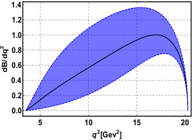
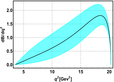
  Figure 2: Branching ratio (in units of $10^{-6}$) of $\Lambda_{b}\to\Lambda\tau^{+}\mu^{-}$ (left) and $\Lambda_{b}\to\Lambda\tau^{-}\mu^{+}$ (right).

  From the differential branching ratio plot, it is evident that both decay modes are expected to have similar order of branching fractions. However, the predicted value of $\mathcal{B}(\Lambda_{b}\to\Lambda\mu^{-}\tau^{+})$ is found to be slightly higher than that of $\mathcal{B}(\Lambda_{b}\to\Lambda\mu^{+}\tau^{-})$.

• Forward-backward asymmetry: Taking into account the lepton forward-backward asymmetry, the $\Lambda_{b}\to\Lambda\tau^{+}\mu^{-}$ decay exhibits a zero crossing in the FBA curve, whereas in the case of $\Lambda_{b}\to\Lambda\tau^{-}\mu^{+}$, no such zero crossing is observed. Such asymmetry curves are shown in Fig. 3. The zero crossing for the former $\Lambda_{b}$ decay occurs at $q^{2}$=12 ${\rm GeV}^{2}$. For $\Lambda_{b}\to\Lambda\tau^{-}\mu^{+}$, the forward backward asymmetry remains negative throughout all $q^{2}$ regions.

  

  

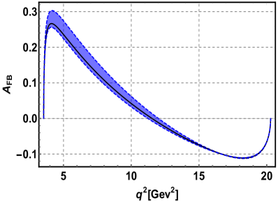
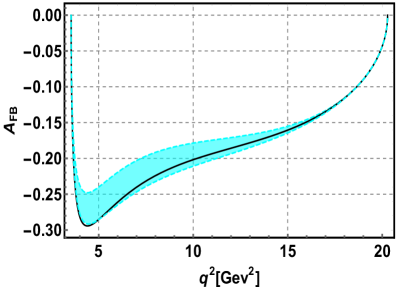
  Figure 3: Forward-backward asymmetry of $\Lambda_{b}\to\Lambda\tau^{+}\mu^{-}$ (left) and $\Lambda_{b}\to\Lambda\tau^{-}\mu^{+}$ (right).

The numerical estimation for the branching ratio and $A_{FB}$ are computed using the central value of the form factors and benchmark points of the SMEFT Wilson coefficient. This has been shown in Table 4. As mentioned before the obtained results correspond to the cut-off scale $\Lambda_{cut}$=1 TeV, and the evolution of the branching ratios of the $\Lambda_{b}\to\Lambda\mu^{\pm}\tau^{\mp}$ with the cut-off scale are shown in the Fig. 4.

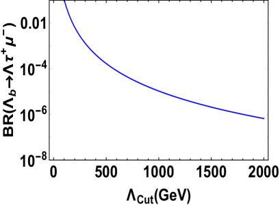
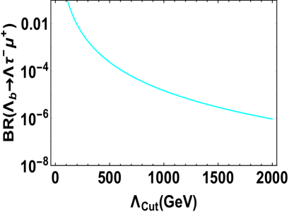
Figure 4: Variation of the branching ratio of $\Lambda_{b}\to\Lambda\tau^{+}\mu^{-}$ (left), $\Lambda_{b}\to\Lambda\tau^{-}\mu^{+}$ (right) with the cut-off scale.

IV.2 Impact of SMEFT NP coefficients on $B\to K_{2}^{*}\ell_{1}\ell_{2}$ decay observables

• Branching ratio: Fig. 5 shows $q^{2}$-dependent differential branching ratios of the $B\to K_{2}^{*}\mu^{\pm}\tau^{\mp}$ processes. The contribution of SMEFT NP couplings is significant in the intermediate invariant mass squared region. The behavior of the differential branching ratios for both decay modes are of similar. However, the value of ${\cal B}(B\to K_{2}^{*}\mu^{+}\tau^{-})$ is higher than that for the ${\cal B}(B\to K_{2}^{*}\mu^{-}\tau^{+})$.

  

  

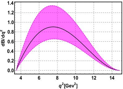
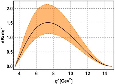
  Figure 5: Branching ratio (in units of $10^{-6}$) of $B\to K_{2}^{*}\mu^{-}\tau^{+}$ (left) and $B\to K_{2}^{*}\mu^{+}\tau^{-}$ (right).

  

  

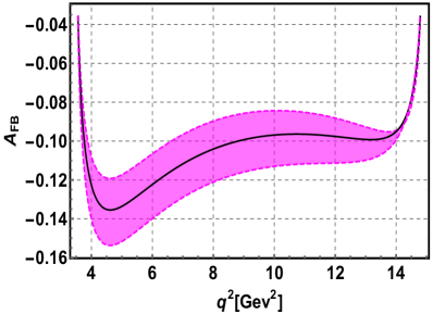
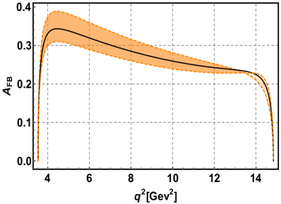
  Figure 6: Forward-backward asymmetry of the $B\to K_{2}^{*}\tau^{+}\mu^{-}$ (left) and $B\to K_{2}^{*}\tau^{-}\mu^{+}$(right).

• Forward-backward asymmetry: Fig. 6 depicts the $q^{2}$ dependency of the forward-backward asymmetry. The two plots illustrate distinct behaviors for the two different decay modes. For $B\to K_{2}^{*}\mu^{-}\tau^{+}$ decay, the observable $A_{FB}$ is negative throughout the entire $q^{2}$ region, while for $B\to K_{2}^{*}\mu^{+}\tau^{-}$ decay, the forward-backward asymmetry remains positive throughout the $q^{2}$ region.

The numerical estimation is given in Table 4, whereas, the cut-off dependent branching fraction is depicted in Fig. (7)

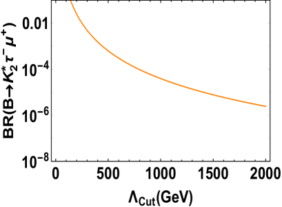
Figure 7: Cut off dependent branching ratio of $B\to K_{2}^{*}\tau^{+}\mu^{-}$ (left) and $B\to K_{2}^{*}\tau^{-}\mu^{+}$ (right).

IV.3 Impact of SMEFT NP coefficients on $B\to(K^{*},\phi)\ell_{1}\ell_{2}$ decay observables

• Branching ratio: The numerical values for the expected branching ratios of the decay process are provided in Table 4. In Fig. 8, we present the $q^{2}$-dependent differential branching ratio of $B_{(s)}\to(K^{*},\phi)\tau^{\pm}\mu^{\mp}$ decay processes. Each mode of $B_{(s)}\to(K^{*},\phi)$ process has almost similar $q^{2}$ dependencies of the differential branching ratio irrespective of the charge of the heavier lepton. Therefore, we have shown a single curve for both modes $\tau^{\pm}\mu^{\mp}$.

  

  

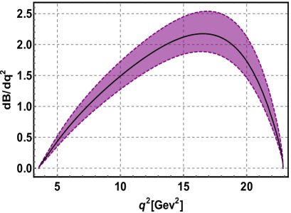
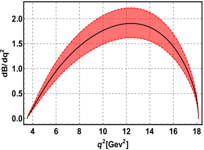
  Figure 8: Branching ratio (in the units of $10^{-6}$) of $B\to K^{*}\tau\mu$ (left) and $B\to\phi\tau\mu$ (right).

• Forward-backward asymmetry: We see no zero crossing for both of the modes irrespective of the charge of heavy lepton. For both $B(B_{s})\to K^{*}(\phi)\tau\mu$ decay, the observable $A_{FB}$ remains positive throughout the $q^{2}$ region. This is shown in Fig. 9. We also provide the prediction for the forward-backward asymmetry for the decay process which is provided in Table 4.

  

  

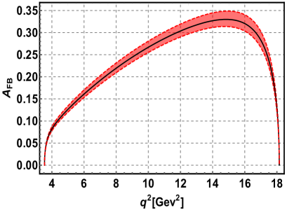
  Figure 9: Forward-backward asymmetry of $B\to K^{*}\tau^{\pm}\mu^{\mp}$ (left) and $B_{s}\to\phi\tau^{\pm}\mu^{\mp}$ (right)

• Longitudinal polarisation asymmetry: The $q^{2}$ dependent lepton longitudinal polarisation asymmetry of $B\to K^{*}\tau\mu$ and $B\to\phi\tau\mu$ decays are shown in Fig. 10. The observables have similar behavior irrespective of the charges of the lepton pair. In addition, the numerical values of $F_{L}$ are also given in the Table 4.

  

  

  Figure 10: Longitudinal polarization asymmetry of $B\to K^{*}\tau\mu$(left)and $B\to\phi\tau\mu$ (right)

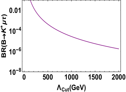
Figure 11: Cutoff dependent branching ratio of $B\to K^{*}\tau\mu$ (left) and $B\to\phi\tau\mu$ (right).

As mentioned earlier, for our numerical computations, we set the cutoff limit $\Lambda_{\rm cut}$=1 TeV. The evolution of the branching ratio for the decay process is depicted in Fig. 11. Similarly the evolution of the $[C^{(1)}_{\ell q}]^{23\ell_{1}\ell_{2}}$ and $[C_{leqd}]^{23\ell_{1}\ell_{2}}$ can be shown similarly.

	$\mathcal{B}$	$\mathcal{A}_{FB}$	$\mathcal{F}_{L}$
$\Lambda_{b}\to\Lambda\tau^{-}\mu^{+}$	$\leq 1.0\times 10^{-5}$	$\leq 0.030$	$-$
$\Lambda_{b}\to\Lambda\tau^{+}\mu^{-}$	$\leq 1.49\times 10^{-5}$	$\leq-0.18$	$-$
$B\to K^{*}\tau\mu$	$\leq 2.805\times 10^{-5}$	$\leq 0.365$	$\leq 0.431$
$B_{s}\to\phi\tau\mu$	$\leq 3.02\times 10^{-5}$	$\leq 0.243$	$\leq 0.564$
$B\to K_{2}^{*}\tau^{+}\mu^{-}$	$\leq 5.856\times 10^{-6}$	$\leq-0.104$	$-$
$B\to K_{2}^{*}\tau^{-}\mu^{+}$	$\leq 9.359\times 10^{-6}$	$\leq 0.271$	$-$

Table 4: Predicted upper limits of $\mathcal{B}$ and $\mathcal{A_{FB}}$ for the $\Lambda_{b}\to\Lambda\tau^{\pm}\mu^{\mp}$, $B\to(K^{*},\phi)\tau^{\pm}\mu^{\mp}$ and $B\to K_{2}^{*}\tau^{\pm}\mu^{\mp}$ decays, with $\mathcal{F_{L}}$ prediction for $B\to(K^{*},\phi)\tau^{\pm}\mu^{\mp}$.

V Conclusion

The observation of any LFV decays indicates a clear signal of the presence of new physics beyond the SM, as such decays are strictly forbidden within its framework. Various extensions of the SM have been proposed to explain the origin of lepton flavor universality-violating couplings. This in turn suggests the presence of lepton flavor-violating decays, thus providing motivating insights to conduct a closer examination of LFV decays. In this work, we have studied the lepton flavor violating $B_{(s)}$ decays based on $b\to s\tau\mu$ transitions. For this purpose, we constrained the parameter space of NP couplings weighted by (pseudo)scalar and axial(vector) operators, by using the the upper limits of Br($B\to\tau\mu$) and Br($B\to K\tau\mu$) in the presence of SMEFT Wilson coefficients. Using such constrained NP parameters, we have investigated the impact on the branching fraction, forward-backward asymmetry and the lepton polarisation asymmetry of the exclusive $B_{(s)}\rightarrow(\phi,K^{*},K_{2}^{*})\tau\mu$ and $\Lambda_{b}\rightarrow\Lambda\tau\mu$ processes. We observed that in the presence of new SMEFT couplings, these observables receive significant contributions. Furthermore, we presented the cut-off scale dependency of the branching ratios for the $b\to s\tau\mu$ decays. Additionally, we made predictions for the upper limits of the aforementioned observables as summarized in Table 4. The findings reveal that our predicted values are substantial and within the reach of current or forthcoming experimental limits. If detected in the experiments in the future, this would offer a definitive indication of new physics.

VI Acknowledgement

DP would like to acknowledge the support of the Prime Minister’s Research Fellowship, Government of India. MKM acknowledges IoE PDRF, University of Hyderabad for the financial support. RM would like to acknowledge the University of Hyderabad IoE project grant no. RC1-20-012.

Appendix A The Angular coefficients of $\Lambda_{b}\to\Lambda\ell_{1}\ell_{2}$ process

The of the angular coefficients $K_{1ss,1cc,1c}$ can be expressed as follows:

$$K_{1ss,1cc}=K_{1ss,1cc}^{VA}+K_{1ss,1cc}^{SP}+K_{1ss,1cc}^{int},$$ (25)

where, the $K_{1ss,1cc}^{VA}$, $K_{1ss,1cc}^{SP}$ and $K_{1ss,1cc}^{int}$ are given as follows,

$$K_{1ss}^{\rm VA} = \frac{1}{4}\bigg{(}2|A_{||0}^{R}|^{2}+|A_{||1}^{R}|^{2}+2|A_{\perp 0}^{R}|^{2}+|A_{||1}^{R}|^{2}+\{R\leftrightarrow L\}\bigg{)}$$ (26)

$$-\frac{m_{+}^{2}+m_{-}^{2}}{4q^{2}}\bigg{[}\bigg{(}|A^{R}_{\|_{0}}|^{2}+|A^{R}_{\perp_{0}}|^{2}+\{R\leftrightarrow L\}\bigg{)}-\bigg{(}|A_{\perp t}|^{2}+\{\perp\leftrightarrow\|\}\bigg{)}\bigg{]}$$

$$+\frac{m_{+}^{2}-m_{-}^{2}}{4q^{2}}\bigg{[}2\rm Re\bigg{(}A^{R}_{\perp_{0}}A^{\ast L}_{\perp_{0}}+A^{R}_{\perp_{1}}A^{\ast L}_{\perp_{1}}+\{\perp\leftrightarrow\|\}\bigg{)}\bigg{]}$$

$$-\frac{m_{+}^{2}m_{-}^{2}}{4q^{4}}\bigg{[}\bigg{(}|A_{\perp 1}^{R}|^{2}+|A_{||1}^{R}|^{2}+\{R\leftrightarrow L\}\bigg{)}+2|A_{\|t}|^{2}+2|A_{\perp t}|^{2}\bigg{]},$$

$$K_{1cc}^{\rm VA} = \frac{1}{2}\bigg{(}|A_{\perp 1}^{R}|^{2}+|A_{||1}^{R}|^{2}+\{R\leftrightarrow L\}\bigg{)}+\frac{m_{+}^{2}+m_{-}^{2}}{4q^{2}}$$ (27)

$$\times\bigg{[}\bigg{(}|A^{R}_{||_{0}}|^{2}-|A^{R}_{||_{1}}|^{2}+|A^{R}_{\perp_{0}}|^{2}-|A^{R}_{\perp_{1}}|^{2}+\{R\leftrightarrow L\}\bigg{)}+\bigg{(}|A_{\perp t}|^{2}+|A_{||t}|^{2}\bigg{)}\bigg{]}$$

$$+\frac{m_{+}^{2}-m_{-}^{2}}{4q^{2}}\bigg{[}2\rm Re\bigg{(}A^{R}_{\perp_{0}}A^{*L}_{\perp_{0}}\ +A^{R}_{\perp_{1}}A^{L}_{\perp_{1}}+\{\perp\leftrightarrow||\}\bigg{)}\bigg{]}$$

$$-\frac{m_{+}^{2}m_{-}^{2}}{2q^{4}}\bigg{[}\bigg{(}|A_{\perp 0}^{R}|^{2}+|A_{||0}^{R}|^{2}+\{R\leftrightarrow L\}\bigg{)}+|A_{||t}|^{2}+|A_{\perp t}|^{2}\bigg{]},$$

$$K_{1c}^{\rm VA} = -\beta_{\ell}\beta_{\ell}^{\prime}\bigg{(}A^{R}_{\perp_{1}}A^{*R}_{||_{1}}-\{R\leftrightarrow L\}\bigg{)}+\beta_{\ell}\beta_{\ell}^{\prime}\frac{m_{+}m_{-}}{q^{2}}\rm Re\bigg{(}A_{||0}^{L}A_{||t}^{*}+A_{\perp 0}^{L}A_{\perp t}^{*}\bigg{)}.$$ (28)

$$K_{1ss}^{\rm SP}=\frac{1}{4}\bigg{(}|A_{\rm S\perp}|^{2}+|A_{\rm P\perp}|^{2}+\{\perp\leftrightarrow\|\}\bigg{)}-\frac{m_{+}^{2}}{4q^{2}}\big{(}|A_{S||}|^{2}+|A_{S\perp}|^{2}\big{)}-\frac{m_{-}^{2}}{4q^{2}}\big{(}|A_{P||}|^{2}+|A_{P\perp}|^{2}\big{)},$$

$$K_{1cc}^{\rm SP}=\frac{1}{4}\bigg{(}|A_{\rm P\perp}|^{2}+|A_{\rm S\perp}|^{2}+\{\perp\leftrightarrow\|\}\bigg{)}-\frac{m_{+}^{2}}{4q^{2}}\big{(}|A_{S||}|^{2}+|A_{S\perp}|^{2}\big{)}-\frac{m_{-}^{2}}{4q^{2}}\big{(}|A_{P||}|^{2}+|A_{P\perp}|^{2}\big{)},$$

$$K_{1c}^{\rm SP}=0.$$ (29)

$$K_{1ss}^{\rm int} = \frac{m_{+}}{2\sqrt{q^{2}}}\rm Re\bigg{(}A_{||t}A_{P||}^{*}+A_{\perp t}A_{P\perp}^{*}\bigg{)}+\frac{m_{-}}{2\sqrt{q^{2}}}Re\bigg{(}A_{||t}A_{S||}^{*}+A_{\perp t}A_{S\perp}^{*}\bigg{)}$$ (30)

$$-\frac{m_{+}^{2}m_{-}}{2q^{2}\sqrt{q^{2}}}Re\bigg{(}A_{||t}A_{S||}^{*}+A_{\perp t}A_{S\perp}^{*}\bigg{)}-\frac{m_{+}m_{-}^{2}}{2q^{2}\sqrt{q^{2}}}Re\bigg{(}A_{||t}A_{P||}^{*}+A_{\perp t}A_{P\perp}^{*}\bigg{)},$$

$$K_{1cc}^{\rm int} = \frac{m_{+}}{2\sqrt{q^{2}}}Re\bigg{(}A_{||t}A_{P||}^{*}+A_{\perp t}A_{P\perp}^{*}\bigg{)}+\frac{m_{-}}{2\sqrt{q^{2}}}Re\bigg{(}A_{||t}A_{S||}^{*}+A_{\perp t}A_{S\perp}^{*}\bigg{)}$$ (31)

$$-\frac{m_{+}^{2}m_{-}}{2q^{2}\sqrt{q^{2}}}Re\bigg{(}A_{||t}A_{S||}^{*}+A_{\perp t}A_{S\perp}^{*}\bigg{)}-\frac{m_{+}m_{-}^{2}}{2q^{2}\sqrt{q^{2}}}Re\bigg{(}A_{||t}A_{P||}^{*}+A_{\perp t}A_{P\perp}^{*}\bigg{)},$$

$$K_{1c}^{\rm int} = \frac{\beta_{\ell}\beta_{\ell}^{\prime}}{2\sqrt{q^{2}}}Re\bigg{(}A_{S||}A_{||0}^{L*}+A_{S\perp}A_{\perp 0}^{L*}+A_{S||}A_{||0}^{R*}+A_{|S\perp}A_{\perp 0}^{R*}\bigg{)}$$ (32)

$$+\frac{\beta_{\ell}\beta_{\ell}^{\prime}}{2\sqrt{q^{2}}}Re\bigg{(}A_{P||}A_{||0}^{L*}+A_{P\perp}A_{\perp 0}^{L*}+-A_{P||}A_{||0}^{R*}-A_{|S\perp}A_{\perp 0}^{R*}\bigg{)}.$$

Here, we have defined $m_{\mp}=m_{1}\mp m_{2}$ with $m_{1},m_{2}$ as the masses of $\ell_{1}$ and $\ell_{2}$, respectively.

Appendix B Inputs required for $B\to K_{2}^{*}\ell_{1}\ell_{2}$ decay mode

$$C(q^{2}) = \frac{3}{8}\beta_{+}^{2}\beta_{-}^{2}\left\{\left(|A_{L}^{\parallel}|^{2}+|A_{L}^{\perp}|^{2}-2|A_{L}^{0}|^{2}\right)+\left(L\to R\right)\right\},$$ (33)

$$B(q^{2}) = \frac{3}{2}\beta_{+}\beta_{-}\left\{\rm Re\left[A_{L}^{\perp*}A_{L}^{\parallel}-(L\to R)\right]+\frac{m_{+}m_{-}}{q^{2}}\rm Re\left[A_{L}^{0*}A_{L}^{t}+(L\to R)\right]\right.$$ (34)

$$\left.+\frac{m_{+}}{\sqrt{q^{2}}}\rm Re\left[A_{S}^{*}(A_{L}^{0}+A_{R}^{0})\right]-\frac{m_{-}}{\sqrt{q^{2}}}\rm Re\left[A_{SP}^{*}(A_{L}^{0}-A_{R}^{0})\right]\right\},$$

$$A(q^{2}) = \frac{3}{4}\left\{\frac{1}{4}\left[\left(1+\frac{m_{+}^{2}}{q^{2}}\right)\beta_{-}^{2}+\left(1+\frac{m_{-}^{2}}{q^{2}}\right)\beta_{+}^{2}\right]\left(|A_{L}^{\parallel}|^{2}+|A_{L}^{\perp}|^{2}+(L\to R)\right)\right.$$ (35)

$$+\frac{1}{2}\left(\beta_{-}^{2}+\beta_{+}^{2}\right)\left(|A_{L}^{0}|^{2}+|A_{R}^{0}|^{2}\right)+\frac{4m_{1}m_{2}}{q^{2}}\rm Re\left[A_{L}^{0*}A_{R}^{0}+A_{L}^{\parallel*}A_{R}^{\parallel}+A_{R}^{\perp}A_{L}^{\perp*}-A_{L}^{t}A_{R}^{t*}\right]$$

$$+\frac{1}{2}\left(\beta_{+}^{2}+\beta_{-}^{2}-2\beta_{+}^{2}\beta_{-}^{2}\right)\left(|A_{L}^{t}|^{2}+|A_{R}^{t}|^{2}\right)+\frac{1}{2}\left(|A_{SP}|^{22}+|A_{S}|^{22}\right)$$

$$+\frac{2m_{-}}{\sqrt{q^{2}}}\beta_{+}^{2}\rm Re\left[A_{S}(A_{L}^{t}+A_{R}^{t})^{*}\right]-\frac{2m_{+}}{\sqrt{q^{2}}}\beta_{-}^{2}\rm Re\left[A_{SP}(A_{L}^{t}-A_{R}^{t})^{*}]\right\}.$$

Appendix C Inputs required for $B\to(K^{*},\phi)\ell_{1}\ell_{2}$ process

The full angular distribution for the decay process can be expressed as

$$\begin{split}\frac{d^{4}B(B\rightarrow\bar{K}^{*}(\rightarrow K\pi)\ell_{\alpha}^{-}\ell_{\beta}^{+})}{dq^{2}dcos\theta_{\ell}dcos\theta_{K}d\phi}=\frac{9}{32\pi}I(q^{2},\theta_{\ell},\theta_{K},\phi),\end{split}$$ (36)

where

$$I(q^{2},\theta_{\ell},\theta_{K},\phi)= I_{1}^{s}(q^{2})\sin^{2}\theta_{K}+I_{1}^{c}(q^{2})\cos^{2}\theta_{K}+[I_{2}^{s}(q^{2})\sin^{2}\theta_{K}+I_{2}^{c}(q^{2})\cos^{2}\theta_{K}]\cos 2\theta_{\ell}$$

$$+I_{3}(q^{2})\sin^{2}\theta_{K}\sin^{2}\theta_{\ell}\cos 2\phi+I_{4}(q^{2})\sin 2\theta_{K}\sin 2\theta_{\ell}\cos\phi$$

$$+I_{5}(q^{2})\sin 2\theta_{K}\sin\theta_{\ell}\cos\phi+[I_{6}^{s}(q^{2})\sin^{2}\theta_{K}+I_{6}^{c}(q^{2})\cos^{2}\theta_{K}]\cos\theta_{\ell}$$

$$+I_{7}(q^{2})\sin 2\theta_{K}\sin\theta_{\ell}\sin\phi+I_{8}(q^{2})\sin 2\theta_{K}\sin 2\theta_{\ell}\sin\phi$$

$$+I_{9}(q^{2})\sin^{2}\theta_{K}\sin^{2}\theta_{\ell}\sin 2\phi,$$ (37)

with $\theta_{\ell}$ , $\theta_{K}$ and $\phi$ varies as $-\pi\leq\theta_{\ell},\theta_{K}\leq\pi$ and $0\leq\phi\leq 2\pi$ respectively.
The angular coefficients in terms of transversity amplitude can be expressed as:

$$I_{1}^{s}(q^{2}) =\frac{4m_{1}m_{2}}{q^{2}}\mathrm{Re}\left(A_{\parallel}^{L}A_{\parallel}^{R\ast}+A_{\perp}^{L}A_{\perp}^{R\ast}\right)+\biggl{[}|A_{\perp}^{L}|^{2}+|A_{\parallel}^{L}|^{2}+(L\to R)\biggr{]}\frac{\lambda_{q}+2[q^{4}-(m_{1}^{2}-m_{2}^{2})^{2}]}{4q^{4}},$$

$$I_{1}^{c}(q^{2}) =\frac{8m_{1}m_{2}}{q^{2}}\mathrm{Re}(A_{0}^{L}A_{0}^{R\ast}-A_{t}^{L}A_{t}^{R\ast})+\bigl{[}|A_{0}^{L}|^{2}+|A_{0}^{R}|^{2}\bigr{]}\frac{q^{4}-(m_{1}^{2}-m_{2}^{2})^{2}}{q^{4}}$$

$$\hskip 99.58464pt-2\frac{(m_{1}^{2}-m_{2}^{2})^{2}-q^{2}(m_{1}^{2}+m_{2}^{2})}{q^{4}}\bigl{(}|A_{t}^{L}|^{2}+|A_{t}^{R}|^{2}\bigr{)},$$

$$I_{2}^{s}(q^{2}) =\frac{\lambda_{q}}{4q^{4}}[|A_{\parallel}^{L}|^{2}+|A_{\perp}^{L}|^{2}+(L\to R)],$$

$$I_{2}^{c}(q^{2}) =-\frac{\lambda_{q}}{q^{4}}(|A_{0}^{R}|^{2}+|A_{0}^{L}|^{2}),$$

$$I_{3}(q^{2}) =\frac{\lambda_{q}}{2q^{4}}[|A_{\perp}^{L}|^{2}-|A_{\parallel}^{L}|^{2}+(L\to R)],$$

$$I_{4}(q^{2}) =-\frac{\lambda_{q}}{\sqrt{2}q^{4}}\mathrm{Re}(A_{\parallel}^{L}A_{0}^{L\ast}+(L\to R)],$$

$$I_{5}(q^{2}) =\frac{\sqrt{2}\lambda_{q}^{1/2}}{q^{2}}\left[\mathrm{Re}(A_{0}^{L}A_{\perp}^{L\ast}-(L\to R))-\frac{m_{1}^{2}-m_{2}^{2}}{q^{2}}\mathrm{Re}(A_{t}^{L}A_{\parallel}^{L\ast}+(L\to R))\right],$$

$$I_{6}^{s}(q^{2}) =-\frac{2\lambda_{q}^{1/2}}{q^{2}}[\mathrm{Re}(A_{\parallel}^{L}A_{\perp}^{L\ast}-(L\to R))],$$

$$I_{6}^{c}(q^{2}) =-\frac{4\lambda_{q}^{1/2}}{q^{2}}\frac{m_{1}^{2}-m_{2}^{2}}{q^{2}}\mathrm{Re}(A_{0}^{L}A_{t}^{L\ast}+(L\to R)),$$

$$I_{7}(q^{2}) =-\frac{\sqrt{2}\lambda_{q}^{1/2}}{q^{2}}\left[\frac{m_{1}^{2}-m_{2}^{2}}{q^{2}}\mathrm{Im}(A_{\perp}^{L}A_{t}^{L\ast}+(L\to R))+\mathrm{Im}(A_{0}^{L}A_{\parallel}^{L\ast}-(L\to R))\right],$$

$$I_{8}(q^{2}) =\frac{\lambda_{q}}{\sqrt{2}q^{4}}\mathrm{Im}(A_{0}^{L}A_{\perp}^{L\ast}+(L\to R)),$$

$$I_{9}(q^{2}) =-\frac{\lambda_{q}}{q^{4}}\mathrm{Im}(A_{\perp}^{R}A_{\parallel}^{R\ast}+A_{\perp}^{L}A_{\parallel}^{L\ast}).$$ (38)

The transversity amplitude can be written as follows Becirevic:2016zri ,

$$A_{\perp}^{L(R)}= {\cal N}_{K^{\ast}}\sqrt{2}\lambda_{B}^{1/2}\left[(C_{9}\mp C_{10})\frac{V(q^{2})}{m_{B}+m_{K^{\ast}}}\right],$$

$$\hskip 5.69054ptA_{\parallel}^{L(R)}= -{\cal N}_{K^{\ast}}\sqrt{2}(m_{B}^{2}-m_{K^{\ast}}^{2})\left[(C_{9}\mp C_{10})\frac{A_{1}(q^{2})}{m_{B}-m_{K^{\ast}}}\right],$$

$$A_{0}^{L(R)}= -\frac{{\cal N}_{K^{\ast}}}{2m_{K^{\ast}}\sqrt{q^{2}}}(C_{9}\mp C_{10})\left[(m_{B}^{2}-m_{K^{\ast}}^{2}-q^{2})(m_{B}+m_{K^{\ast}})A_{1}(q^{2})-\frac{\lambda_{B}A_{2}(q^{2})}{m_{B}+m_{K^{\ast}}}\right],$$

$$A_{t}^{L(R)}= -{\cal N}_{K^{\ast}}\frac{\lambda_{B}^{1/2}}{\sqrt{q^{2}}}\left[(C_{9}\mp C_{10})+\frac{q^{2}}{m_{b}+m_{s}}\left(\frac{C_{S}}{m_{1}-m_{2}}\mp\frac{C_{P}}{m_{1}+m_{2}}\right)\right]A_{0}(q^{2}).$$ (39)

where,

$$N_{K^{*}}= V_{tb}V_{ts}^{*}\bigg{[}\frac{\tau_{B_{d}}G_{F}^{2}\alpha_{em}^{2}\sqrt{\lambda_{B}\lambda_{q}}}{3\times 2^{10}\pi^{5}m_{B}^{3}}\bigg{]}^{\frac{1}{2}},$$

$$\lambda(a^{2},b^{2},c^{2})= a^{4}+b^{4}+c^{4}-2(a^{2}b^{2}+b^{2}c^{2}+c^{2}a^{2}).$$ (40)

In the above equation, $G_{F}$ is the Fermi coupling constant whereas $\tau_{B_{d}}$ represents the life time of $B_{d}$ meson. The term proportional to $V_{tb}V_{ts}$ survives in the SM limit.

References

- (1) R. Aaij et al., “Test of lepton universality in decays,” Phys. Rev. Lett., vol. 131, no. 5, p. 051803, 2023.
- (2) R. Aaij et al., “Measurement of lepton universality parameters in and decays,” Phys. Rev. D, vol. 108, no. 3, p. 032002, 2023.
- (3) R. Aaij et al., “Measurement of Form-Factor-Independent Observables in the Decay ,” Phys. Rev. Lett., vol. 111, p. 191801, 2013.
- (4) R. Aaij et al., “Angular analysis of the decay using 3 fb-1 of integrated luminosity,” JHEP, vol. 02, p. 104, 2016.
- (5) M. Aaboud et al., “Angular analysis of decays in collisions at TeV with the ATLAS detector,” JHEP, vol. 10, p. 047, 2018.
- (6) R. Aaij et al., “Tests of lepton universality using and decays,” Phys. Rev. Lett., vol. 128, no. 19, p. 191802, 2022.
- (7) R. Aaij et al., “Branching Fraction Measurements of the Rare and - Decays,” Phys. Rev. Lett., vol. 127, no. 15, p. 151801, 2021.
- (8) C.-J. Lee and J. Tandean, “Minimal lepton flavor violation implications of the anomalies,” JHEP, vol. 08, p. 123, 2015.
- (9) W. Altmannshofer and I. Yavin, “Predictions for lepton flavor universality violation in rare B decays in models with gauged ,” Phys. Rev. D, vol. 92, no. 7, p. 075022, 2015.
- (10) A. Crivellin, G. D’Ambrosio, and J. Heeck, “Explaining , and in a two-Higgs-doublet model with gauged ,” Phys. Rev. Lett., vol. 114, p. 151801, 2015.
- (11) R. Alonso, B. Grinstein, and J. Martin Camalich, “Lepton universality violation and lepton flavor conservation in -meson decays,” JHEP, vol. 10, p. 184, 2015.
- (12) S. Sahoo and R. Mohanta, “Lepton flavor violating B meson decays via a scalar leptoquark,” Phys. Rev. D, vol. 93, no. 11, p. 114001, 2016.
- (13) S. Sahoo and R. Mohanta, “Scalar leptoquarks and the rare meson decays,” Phys. Rev. D, vol. 91, no. 9, p. 094019, 2015.
- (14) M. K. Mohapatra, L. Nayak, R. Dhamija, and A. Giri, “Delving into the , processes,” 2 2023.
- (15) M. I. Ali, U. Chattopadhyay, N. Rajeev, and J. Roy, “SMEFT analysis of charged lepton flavor violating -meson decays,” 12 2023.
- (16) R. Aaij et al., “Search for the lepton-flavour-violating decays and ,” Phys. Rev. Lett., vol. 123, no. 21, p. 211801, 2019.
- (17) R. Aaij et al., “Search for Lepton-Flavor Violating Decays ,” Phys. Rev. Lett., vol. 123, no. 24, p. 241802, 2019.
- (18) S. Watanuki et al., “Search for the Lepton Flavor Violating Decays B+→K+ (=e, ) at Belle,” Phys. Rev. Lett., vol. 130, no. 26, p. 261802, 2023.
- (19) R. Aaij et al., “Search for the lepton-flavour violating decays ,” JHEP, vol. 06, p. 143, 2023.
- (20) D. Das, “Lepton flavor violating decay,” Eur. Phys. J. C, vol. 79, no. 12, p. 1005, 2019.
- (21) D. Das, “Model independent New Physics analysis in decay,” Eur. Phys. J. C, vol. 78, no. 3, p. 230, 2018.
- (22) T. Feldmann and M. W. Y. Yip, “Form factors for transitions in the soft-collinear effective theory,” Phys. Rev. D, vol. 85, p. 014035, 2012. [Erratum: Phys.Rev.D 86, 079901 (2012)].
- (23) W. Detmold and S. Meinel, “ form factors, differential branching fraction, and angular observables from lattice QCD with relativistic quarks,” Phys. Rev. D, vol. 93, no. 7, p. 074501, 2016.
- (24) W. Wang, “B to tensor meson form factors in the perturbative QCD approach,” Phys. Rev. D, vol. 83, p. 014008, 2011.
- (25) T. M. Aliev, H. Dag, A. Kokulu, and A. Ozpineci, “ transition form factors in light-cone sum rules,” Phys. Rev. D, vol. 100, no. 9, p. 094005, 2019.
- (26) S. Kumbhakar, R. Sain, and J. Vardani, “Lepton flavor violating decays,” J. Phys. G, vol. 50, no. 9, p. 095003, 2023.
- (27) J. G. Korner and G. A. Schuler, “Exclusive Semileptonic Heavy Meson Decays Including Lepton Mass Effects,” Z. Phys. C, vol. 46, p. 93, 1990.
- (28) D. Bečirević, O. Sumensari, and R. Zukanovich Funchal, “Lepton flavor violation in exclusive decays,” Eur. Phys. J. C, vol. 76, no. 3, p. 134, 2016.
- (29) A. Bharucha, D. M. Straub, and R. Zwicky, “ in the Standard Model from light-cone sum rules,” JHEP, vol. 08, p. 098, 2016.
- (30) B. Grzadkowski, M. Iskrzynski, M. Misiak, and J. Rosiek, “Dimension-Six Terms in the Standard Model Lagrangian,” JHEP, vol. 10, p. 085, 2010.
- (31) R. Aaij et al., “Search for the lepton flavour violating decay using decays,” JHEP, vol. 06, p. 129, 2020.
- (32) J. P. Lees et al., “A search for the decay modes ,” Phys. Rev. D, vol. 86, p. 012004, 2012.
- (33) D. Bečirević, N. Košnik, O. Sumensari, and R. Zukanovich Funchal, “Palatable Leptoquark Scenarios for Lepton Flavor Violation in Exclusive modes,” JHEP, vol. 11, p. 035, 2016.
- (34) J. Gratrex, M. Hopfer, and R. Zwicky, “Generalised helicity formalism, higher moments and the angular distributions,” Phys. Rev. D, vol. 93, no. 5, p. 054008, 2016.
- (35) P. A. Zyla et al., “Review of Particle Physics,” PTEP, vol. 2020, no. 8, p. 083C01, 2020.
- (36) UTfit-collaboration. http://www.utfit.org/UTfit/WebHome.
- (37) R. Balasubramamian and B. Blossier, “Decay constant of and mesons from lattice QCD,” Eur. Phys. J. C, vol. 80, no. 5, p. 412, 2020.
- (38) M. Bordone, M. Rahimi, and K. K. Vos, “Lepton flavour violation in rare decays,” Eur. Phys. J. C, vol. 81, no. 8, p. 756, 2021.
- (39) M. Algueró, B. Capdevila, S. Descotes-Genon, J. Matias, and M. Novoa-Brunet, “ global fits after and ,” Eur. Phys. J. C, vol. 82, no. 4, p. 326, 2022.
- (40) W. Altmannshofer and P. Stangl, “New physics in rare B decays after Moriond 2021,” Eur. Phys. J. C, vol. 81, no. 10, p. 952, 2021.
- (41) T. Hurth, F. Mahmoudi, D. M. Santos, and S. Neshatpour, “More Indications for Lepton Nonuniversality in ,” Phys. Lett. B, vol. 824, p. 136838, 2022.
- (42) M. Ciuchini, A. M. Coutinho, M. Fedele, E. Franco, A. Paul, L. Silvestrini, and M. Valli, “New Physics in confronts new data on Lepton Universality,” Eur. Phys. J. C, vol. 79, no. 8, p. 719, 2019.