Curvature of the chiral phase transition line from the magnetic equation of state of -flavor QCD
Abstract
We analyze the dependence of the chiral phase transition temperature on baryon number and strangeness chemical potentials by calculating the leading order curvature coefficients in the light and strange quark flavor basis as well as in the conserved charge () basis. Making use of scaling properties of the magnetic equation of state (MEoS) and including diagonal as well as off-diagonal contributions in the expansion of the energy-like scaling variable that enters the parametrization of the MEoS, allows to explore the variation of along different lines in the plane. On lattices with fixed cut-off in units of temperature, , we find , and . We show that the chemical potential dependence along the line of vanishing strangeness chemical potential is about 10% larger than along the strangeness neutral line. The latter differs only by about from the curvature on a line of vanishing strange quark chemical potential, . We also show that close to the chiral limit the strange quark mass contributes like an energy-like variable in scaling relations for pseudo-critical temperatures. The chiral phase transition temperature decreases with decreasing strange quark mass, .
pacs:
11.10.Wx, 11.15.Ha, 12.38.Aw, 12.38.Gc, 12.38.Mh, 24.60.Ky, 25.75.Gz, 25.75.NqI Introduction
The chiral phase transition in Quantum Chromodynamics (QCD) at finite temperature and vanishing chemical potentials is intensively studied in lattice QCD calculations. For QCD with physical (degenerate) up and down quark masses and a strange quark mass tuned to its physical value, it is well established that the transition from the low temperature hadronic phase to a high temperature regime, in which quarks and gluons are the dominant degrees of freedom, is continuous and occurs at a pseudo-critical temperature, MeV Bazavov et al. (2019)111 Pseudo-critical temperatures are not unique. They depend on the observable used to determine them. The value quoted here is obtained by averaging over results obtained with several observables. The spread of results for pseudo-critical temperatures is taken into account in the error quoted. Results obtained from maxima in chiral susceptibilities only Bhattacharya et al. (2014); Borsanyi et al. (2020) are consistent with this result.. A second order phase transition occurs in the limit of vanishing up and down quark masses, , at a temperature MeV Ding et al. (2019). A determination of using twisted mass Wilson fermions is consistent with this finding, MeV Kotov et al. (2021), while a recent analytic calculation, using functional renormalization group methods, gives a somewhat larger critical temperature, MeV Braun et al. (2023).
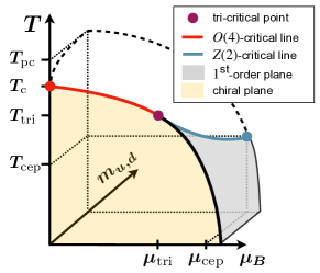
In Fig. 1 we show a sketch of the current understanding of the phase diagram in (2+1)-flavor QCD. The existence of a second order phase transition point in QCD at vanishing light quark masses ( and vanishing chemical potentials (), or correspondingly at vanishing baryon number () and strangeness () chemical potentials is strongly supported by several lattice QCD calculations Ding et al. (2019); Cuteri et al. (2021). However, the existence of a tri-critical point ( in the plane of vanishing light quark masses, (yellow plane in Fig. 1), is still based on model calculations Halasz et al. (1998); Hatta and Ikeda (2003); Stephanov (2006); Buballa and Carignano (2019). At the line of second order chiral phase transitions emerging from , will meet with a line of first order transitions for and a line of second order transitions for . A plane of first order transitions (grey plane in Fig. 1) is bounded by these two lines.
The so-called critical endpoint at , which is expected to exist at physical values of the quark masses, is just one point on the line of second order phase transitions emerging from . It belongs to the , universality class. The nature of the line of second order phase transitions, connecting and , is not yet settled in detail. Although the universality class is expected to be that of , spin models Pisarski and Wilczek (1984), which also is supported through lattice QCD calculations, this is not yet confirmed in detail and a possible larger symmetry group cannot be ruled out as long as the influence of QCD axial symmetry, its explicit breaking at vanishing temperature and effective restoration in the vicinity of , on the QCD phase transition remains controversial Pisarski and Wilczek (1984); Butti et al. (2003); Buchoff et al. (2014); Pelissetto and Vicari (2013); Resch et al. (2019); Aoki et al. (2021); Ding et al. (2021, 2023); Kovacs (2023).
Establishing the existence and determining the location of the critical endpoint at non-vanishing values of quark masses and chemical potentials is of great importance for our understanding of the QCD phase diagram and its phenomenological implications. It has been pointed out Karsch (2019) that the chiral phase transition temperature, , as well as the tri-critical temperature , are expected to give upper bounds for the temperature at the possibly existing critical endpoint in QCD with physical values of the quark masses and non-vanishing baryon chemical potential. As such it is evident that it is of interest to also get control over the dependence of the chiral phase transition on chemical potentials Allton et al. (2002). It will allow to strengthen the bound on .
In this work we will analyze the influence of non-vanishing chemical potentials , that couple to the conserved charge operators for net baryon number and strangeness . We do not include an explicit dependence on an electric charge chemical potential as this would explicitly violate the chiral flavor symmetry in the light quark sector of QCD.
For non-zero , the pseudo-critical as well as the chiral phase transition temperatures shift to smaller values. When considering the case of either a single non-vanishing chemical potential, , or the case where the strangeness chemical potential is constrained, e.g. by demanding an overall vanishing of the net strangeness density, , the shift of pseudo-critical and critical temperatures is, to leading-order, quadratic in and is controlled by the so-called curvature coefficient , which has been determined in calculations with physical (degenerate) light quark masses and a physical strange quark mass Kaczmarek et al. (2011); Bonati et al. (2015); Bellwied et al. (2015); Cea et al. (2016); Bazavov et al. (2019); Bonati et al. (2018); Borsanyi et al. (2020). In the case of non-zero with constrained by demanding vanishing strangeness density () and a ratio of net electric charge to baryon-number density that is appropriate for the description of dense media created in heavy ion collisions (), the curvature coefficient is found to be Bazavov et al. (2019); D’Elia (2019); Borsanyi et al. (2020). Moreover, the next order correction has been found to be consistent with zero Bazavov et al. (2019); Borsanyi et al. (2020), which also is in line with recent model calculations Biswas et al. (2024).
When mapping out the critical surface as function of several non-vanishing chemical potentials, e.g. , also off-diagonal curvature coefficients, e.g. , need to be taken into account. We will discuss here the dependence of various curvature coefficients on the value of two degenerate light quark masses with the strange quark mass tuned to its physical value, aiming at an extrapolation to the chiral limit. In this study we do not yet try to extrapolate to the continuum limit. All calculations are performed at finite values of the lattice cut-off. We will determine diagonal and off-diagonal curvature coefficients, , and , in the conserved charge basis, , as well as the related curvature coefficients , and , in the quark flavor basis .
Close to the chiral limit, universal scaling relations allow the determination of the chiral phase transition temperature and its dependence on, e.g., the chemical potentials, which are a particular set of energy-like scaling fields coupled to energy-like observables Clarke et al. (2021). We will use a scaling ansatz for chiral observables to extract the curvature coefficients and , ignoring regular or sub-leading universal, correction-to-scaling contributions. This ansatz becomes exact when approaching the chiral limit.
This paper is organized as follows. In Section II we present some details on the calculational set up used for this work. In Section III we introduce several chiral observables and discuss universal properties of (2+1)-flavor QCD near the chiral limit. Section IV gives an update on the determination of the chiral phase transition temperature at vanishing chemical potentials, using three sets of susceptibilities that define three different sets of pseudo-critical temperatures. In this section we also present a determination of the non-universal scale parameter , which is needed to define the leading universal part of chiral observables entering the magnetic equation of state. In Section V we present our results on curvature coefficients calculated in conserved charge and conserved flavor basis. Section VI is devoted to a discussion of the dependence of the chiral phase transition temperature on the value of the strange quark mass. We finally give our conclusions in Section VII. In two appendices we give some details on the determination of the leading order coefficient that relates the strangeness and baryon chemical potentials in strangeness neutral systems, followed by a discussion about the sub-leading correction-to-scaling terms that contribute to all thermodynamic observables close to the chiral limit.
II Calculational setup
We consider (2+1)-flavor QCD with a strange quark mass tuned to its physical value and degenerate up and down quark masses, (), that shall be changed to smaller-than-physical values, starting from , including the physical value, and reaching the smallest quark mass ratio . We introduce the chemical potentials for each quark flavor. The partition function, defined on a Euclidean space-time lattice of size , is given as
| (1) |
where and denotes the staggered fermion matrix for quark flavor ; , of course, also is a function of the quark masses , which we have not specified explicitly. Temperature and volume are related to the temporal () and spatial () extent of the lattice with lattice spacing being controlled by the gauge coupling222The gauge coupling , introduced here, should not be confused with the critical exponent that is used frequently in this work. .
| [MeV] | #configurations | |||||
|---|---|---|---|---|---|---|
| 6.245 | 0.0830 | 134.84 | 123004 | – | – | – |
| 6.260 | 0.0810 | 136.98 | – | 71824 | – | – |
| 6.285 | 0.0790 | 140.62 | 145814 | 71547 | 28703 | 13254 |
| 6.300 | 0.0772 | 142.85 | – | 71514 | 28464 | 13299 |
| 6.315 | 0.0759 | 145.11 | 145179 | 71571 | 31754 | 15693 |
| 6.330 | 0.0746 | 147.40 | – | 70212 | 31751 | 15634 |
| 6.354 | 0.0728 | 151.14 | 125679 | 51135 | 31561 | 13200 |
| 6.365 | 0.0716 | 152.88 | – | 49879 | – | – |
| 6.372 | 0.0711 | 154.00 | – | – | 17222 | 13790 |
| 6.390 | 0.0694 | 156.92 | 97526 | 51707 | 17794 | 10129 |
| 6.423 | 0.0670 | 162.39 | 131200 | 52051 | 10917 | 9137 |
| 6.445 | 0.0652 | 166.14 | 176361 | 50689 | 10863 | 9479 |
| 6.474 | 0.0632 | 171.19 | 232116 | 28080 | – | – |
| 6.500 | 0.0614 | 175.84 | 151606 | 29505 | – | – |
For the purpose of the calculations presented here we substantially extended the set of gauge field ensembles generated previously at smaller-than-physical light quark masses for the determination of the chiral phase transition temperature Ding et al. (2019). We use a temperature independent normalization for the chiral symmetry breaking parameter, which is proportional to the degenerate light quark masses , i.e. we use the light quark mass in units of the strange quark mass, . Some preliminary results on the curvature of the chiral phase transition line in the limit have been presented already in Kaczmarek et al. (2022).
All new calculations have been performed on lattices with temporal extent and several spatial lattice sizes with aspect ratio varying between 4 and 7. We vary in order to ensure that the unnormalized (bare) finite-size scaling variable,
| (2) |
stays small. In our calculations we have , except for the smallest quark mass ratio , where . In our previous analysis of critical behavior in (2+1)-flavor QCD Ding et al. (2019) the region has been found to correspond to a region where finite volume effects are small. We discuss the possible influence of finite volume effects in our data for in the next sections. In terms of the pion mass these values for correspond to physical volumes of size . The values for are also given in Table 1.
The gauge field ensembles, used in our study, have been generated with the Highly Improved Staggered Quark (HISQ) action Follana et al. (2007) with tree-level coefficients and a tree-level Symanzik improved gauge action, previously used by us also in calculations with a physical strange quark mass and two degenerate, physical light quark masses Bazavov et al. (2012); Bollweg et al. (2021). The ensembles were generated with a strange quark mass tuned to its physical value and five values of the degenerate light quark masses corresponding to light to strange quark mass ratios, , 1/27, 1/40, 1/80 and 1/160. In the continuum limit these quark mass ratios correspond to light pseudo-scalar pion masses, MeV, 140 MeV, 110 MeV, 80 MeV and 55 MeV, respectively. Using this set-up on lattices with temporal extent , the chiral phase transition temperature has been determined previously to be MeV Ding et al. (2019). We give an update on this value in Sec. IV.2.
For scale setting we use a parametrization of the -function of (2+1)-flavor QCD with physical light and strange quark masses given in Bollweg et al. (2021). The scale is set using the kaon decay constant MeV Aoki et al. (2020).
We summarize details on our simulation parameters and the number of gauge field configurations used in these calculations in Table 1. Data for the largest quark mass ratio, , have been taken from Table XI of Bazavov et al. (2012).
All our numerical calculations are done at vanishing values of the chemical potentials using the simulation package SIMULATeQCD Bollweg et al. (2022); Mazur et al. (2023). Thermodynamic observables at non-vanishing values of the chemical potentials are calculated using the Taylor expansion approach Gavai and Gupta (2003); Allton et al. (2005); Bazavov et al. (2019).
III Chiral observables
III.1 Chiral order parameter
Starting point for our determination of the chiral phase transition temperature and its dependence on quark masses and various chemical potentials is a set of unrenormalized chiral condensates () for flavor , and the related chiral susceptibilities (),
| (3) | |||||
| (4) |
We also introduce the unrenormalized 2-flavor light quark condensate and its susceptibility as the sum of the corresponding up and down quark chiral observables, i.e.
| (5) | |||||
| (6) |
The chiral condensates require multiplicative and additive renormalization to be well defined in the continuum limit. We take care of the multiplicative renormalization by multiplying the light quark chiral condensate with the strange quark mass. Furthermore, we divide by appropriate powers of to define a dimensionless order parameter and its susceptibility,
| (7) | |||||
| (8) |
Additive UV divergences in the chiral condensates are proportional to the quark masses. They can be eliminated by subtracting a suitable observable that contains the same UV divergence. Commonly used is the so-called 2-flavor subtracted chiral condensate () Cheng et al. (2008); Ejiri et al. (2009), which is obtained by subtracting an appropriate fraction of the strange quark condensate from the light quark condensate,
| (9) |
Another possibility to introduce an order parameter for chiral symmetry restoration is to subtract from the light quark condensate a fraction of the corresponding light quark susceptibility,
| (10) |
This version of a renormalized order parameter has the advantage of not involving explicit contributions from the strange quark condensate, which potentially contains larger regular contributions. Moreover, is directly related to a combination of universal scaling functions, which leads to pseudo-critical temperatures that have a weaker quark mass dependence than the chiral susceptibility or other mixed susceptibilities. In the following we will use the unrenormalized order parameter as well as the renormalized order parameters and to define various renormalized susceptibilities that can be used to define pseudo-critical temperatures at non-vanishing .
Finally, we also introduce a mixed susceptibility that is sensitive to changes in the light quark condensate arising from variations of the strange quark mass,
| (11) |
III.2 Chiral and mixed susceptibilities
For the determination of the dependence of the chiral phase transition temperature, , on chemical potentials we will calculate pseudo-critical temperatures that are defined as the location of maxima in various susceptibilities.
As the quadratic UV divergence, present in the unsubtracted order parameter , neither depends on temperature nor on chemical potentials, these divergences are removed when considering susceptibilities obtained as derivatives with respect to or chemical potentials, respectively.
We thus consider in the following several mixed susceptibilities obtained from derivatives of with respect to or with or ,
| (12) | |||||
| (13) | |||||
| (14) |
Here and indicate that derivatives of the order parameter with respect to or temperature like variables and are taken. A corresponding set of susceptibilities can be defined by replacing by the renormalized order parameter or . We will use in the following the mixed susceptibility
| (15) |
Related to the two versions of a renormalized chiral order parameter, and , we introduce two versions of chiral susceptibilities, i.e. the derivatives of or with respect to the light quark mass ,
| (16) | |||||
| (17) |
In the following we will only make use of as the calculation of would require the calculation of three derivatives of the with respect to the light quark masses.
III.3 Universal critical behavior
At vanishing values of the chemical potentials the existence of a continuous order phase transition, occurring at vanishing values of the two degenerate light quark masses, , has been established Ding et al. (2019); Cuteri et al. (2021). As the chemical potentials do not explicitly break the chiral symmetry, the point is part of a surface of order phase transitions that occur at temperatures, . In the vicinity of this critical surface the free energy density, , can be split into a singular contribution and sub-leading corrections that are of relevance in some range of ,
| (18) |
with and . The singular part gives rise to divergences in higher order derivatives of the free energy density. The sub-leading corrections involve non-singular, regular terms as well as sub-dominant, universal singular corrections-to-scaling (cts).
In the vicinity of the critical surface the leading singular contribution to the free energy density dominates the behavior of the chiral and mixed susceptibilities. The dominant singular contribution is written in terms of energy-like and magnetization-like scaling fields, and , respectively. The former couples to operators in the QCD Lagrangian, which are invariant under chiral transformations in the light, degenerate 2-flavor sector and is a function of all combinations of couplings (parameters) appearing in the QCD Lagrangian, which leave the Lagrangian invariant under chiral rotations. The latter, on the other hand, depends on combinations of couplings that break this symmetry. The scaling fields and vanish at a critical point. In its vicinity they may be expanded in a Taylor series. Usually one uses only the leading order Taylor series expansion, , , with
| (19) | |||||
| (20) |
Here , are dimensionless non-universal constants just like , and
| (21) |
In Eq. 19 we introduced the reduced temperature as function of the energy-like couplings and chemical potentials in the flavor basis. This may as well be done in the conserved charge basis using the chemical potentials . Note that we do not include the isospin or electric charge chemical potential in since this amounts to introducing independent up and down quark chemical potentials which explicitly breaks the symmetry group to .
Up to the sub-leading contributions from corrections-to-scaling and contributions from regular terms, the temperature and mass dependence of the singular part of the free energy density is controlled by a single scaling variable ,
| (22) |
with and
| , | (23) |
The critical exponents , are unique in the universality class of the phase transition. As we consider in the following the chiral limit taken at fixed lattice cut-off, we use for definiteness critical exponents of the , universality class, i.e. we use Engels et al. (2000),
| (24) |
Here we give in addition to the two critical exponents also the combination , with and denoting the sub-leading universal correction-to-scaling exponent Hasenbusch and Toeroek (1999); Engels et al. (2000). The combination controls the cts contribution to the order parameters or , respectively.
The scaling functions and , which control the universal, singular parts of the order parameter and its susceptibilities, are related to ,
| (25) | |||||
| (26) |
Taking into account the temperature independent normalization, which we introduced in Eqs. 7, 8, we get for the unsubtracted order parameter, , as well as the renormalized order parameter introduced in Eq. 9,
| (27) |
The universal part of the order parameter , introduced in Eq. 10, is related to the difference of the scaling functions and ,
| (28) |
Correspondingly the mixed susceptibilities, obtained as temperature derivatives of these order parameters, have different universal, singular parts,
| (29) | |||||
Furthermore, the singular part of the chiral susceptibility , introduced in Eq. 16, is controlled by the scaling function ,
| (30) |
Close to contributions arising from corrections-to-scaling give the dominant sub-leading contribution to the order parameter. This contribution is proportional to , while regular terms are proportional to . The correction-to-scaling term thus leads to a sub-leading, still divergent contribution, in susceptibilities.
Close to the chiral limit, where corrections-to-scaling and regular contributions can be neglected, the pseudo-critical temperature, deduced from the maximum of , is related to the maximum of . The maxima of the mixed susceptibilities obtained from derivatives of or with respect to temperature-like couplings, on the other hand, are related to maxima of the scaling functions and , respectively.
These maxima occur at specific values of the scaling variable , which we denoted by for the maximum of , for that of , and for the maximum of the difference . Results for these -values in the , universality class are obtained from the scaling functions given in Karsch et al. (2023),
| (31) | |||||
| (32) | |||||
| (33) |
These specific values of then define pseudo-critical temperatures, obtained from the maxima of the magnetization-like susceptibility or those obtained from the mixed susceptibilities (, as well as . They give rise to three sets of pseudo-critical temperatures. Their leading, universal parts are given by
| (34) | |||||
For Eq. 34 defines the surface of critical temperatures, , spanned by the light and strange quark chemical potentials, respectively.
IV Magnetic equation of state and pseudo-critical temperatures at
As we will exploit the structure of the singular part of the QCD free energy to determine the dependence of the chiral phase transition temperature on chemical potentials, we need as input the non-universal scales and at . These have been determined previously Ding et al. (2019). We will improve here our analysis on lattices with temporal extent making use of our increased statistics at several parameter values.
We will analyze the scaling behavior of the renormalized order parameter and extract pseudo-critical temperatures from the chiral and various mixed susceptibilities introduced in the previous sections.
IV.1 Renormalized order parameter
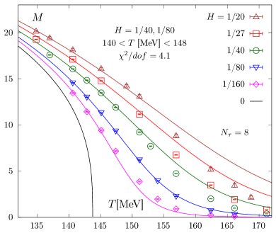
In Fig. 2 (left) we show results for the renormalized order parameter introduced in Eq. 10. Results have been obtained at five different values of on lattices with temporal extent . We fitted these data to the universal scaling ansatz
| (35) |
with and denoting scaling functions in the , universality class Karsch et al. (2023). The scaling functions used in the fit are expressed in the Schofield parametrisation obtained in Karsch et al. (2023). This ansatz involves three fit parameters, (). As we do not include contributions from regular or sub-leading universal terms in this fit we need to restrict the fit to small quark masses and a temperature region close to the pseudo-critical temperature. This has also been done in earlier analyses of the magnetic equation of state Ejiri et al. (2009). It should be noted that in regular contributions to the leading dependent term gets cancelled, leaving only a weaker dependent contribution arising from regular terms.
We fitted the scaling ansatz, Eq. 35, to data for obtained with light to strange quark mass ratios and in the temperature interval with and , respectively. These fits have been performed with and without including the data for the smallest quark mass , which have been obtained on our smallest physical volume and may still suffer somewhat from finite volume effects. The resulting fit parameters are given in Table 2. As can be seen the fit parameters vary little, although the of the fits is quite sensitive to the chosen fit-interval and the range of -values used in the fit.
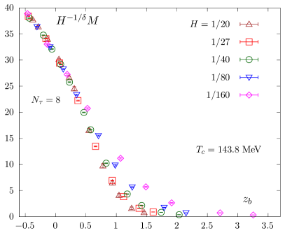
In Fig. 2 (right) we show the rescaled order parameter as function of the scaling variable introduced in Eq. 23. As can be seen, scaling holds well at least up to . For our smallest quark mass ratio, , this corresponds to a temperature interval , which is similar to that finally used also in Ejiri et al. (2009).
| (40,80) | [140:146] | 143.6(1) | 1.39(2) | 39.4(2) | 1.2 |
|---|---|---|---|---|---|
| (40,80) | [140:148] | 143.8(2) | 1.45(3) | 39.0(3) | 4.1 |
| (40,80,160) | [140:146] | 143.6(1) | 1.36(3) | 39.4(2) | 3.7 |
| (40,80,160) | [140:148] | 143.8(2) | 1.40(4) | 38.8(4) | 15.1 |
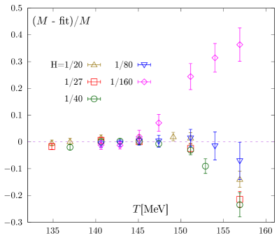
The fits performed in a small temperature interval and for small values of still provide a good description of our data sets for larger and smaller masses as well as for data outside the temperature range used in the fits. Deviations of data outside the fit range from the fit prediction provide an estimate for the influence of regular or sub-leading universal contributions. In Fig. 3 we show the relative deviation of data from the fit also outside the actual fit interval. This suggests that corrections to universal scaling behavior arising from regular or sub-leading universal terms remain smaller than 10% for .
In the following we use the average of the fit results for obtained by leaving out the data for in the fit. We take care of this data set by including the differences as systematic error contributing to the quoted error for . We use,
| (36) | |||||
| (37) | |||||
| (38) |
Using the fit result for the scale parameter , we also conclude from the rescaled order parameter data, shown in Fig. 2 (left), that the parameter range in which we find good scaling behavior without including sub-leading corrections in our fits, corresponds to the region . This suggests that the peak positions of mixed susceptibilities are only mildly influenced by contributions from sub-leading corrections to the dominant universal scaling behavior, as , are of similar magnitude (see Eqs. 32, 33). On the other hand, their influence on the location of the peak of the chiral susceptibility will be larger, as the peak is located at (Eq. 31). We will analyze this in more detail in the next subsection.
| Pseudo-critical temperatures in units of MeV | ||||||
|---|---|---|---|---|---|---|
| observable | ||||||
| (i) | 164.63(5) | 160.99(12) | 157.89(27) | 153.91(30) | 150.93(34) | |
| (ii) | 162.84(28) | 159.76(12) | 155.66(09) | 151.29(14) | 147.92(14) | |
| – | 159.39(22) | 156.38(25) | 150.51(63) | 148.48(74) | ||
| – | 159.94(32) | 156.07(33) | 150.7(1.6) | 148.7(1.2) | ||
| – | 162.76(26) | 159.32(29) | 153.6(96) | 149.87(54) | ||
| (iii) | 156.40(68) | 153.44(11) | 150.70(06) | 148.04(12) | 145.85(17) | |
IV.2 Pseudo-critical temperatures
As we exploit in our determination of the chiral critical surface, scaling relations, which are valid at small values of the symmetry breaking parameter , it is worthwhile to analyze first the behavior of pseudo-critical temperatures at vanishing chemical potentials.
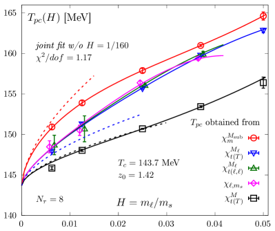
As pointed out in the previous section pseudo-critical temperatures are not unique. Using extrema in second derivatives of the partition function with respect to either (i) the external field coupling , or (ii) mixed derivatives with respect to and one of the temperature-like couplings (), or (iii) by using the temperature derivative of a particular renormalized version of the order parameter, we define three classes of pseudo-critical temperatures333In general one can also determine a pseudo-critical temperature from the susceptibility obtained as second derivative with respect to temperature (specific heat). However, in the universality class, this susceptibility does not diverge as the relevant critical exponent is negative., which converge for to the uniquely defined critical temperature . In the universal scaling region these three sets of observables yield three different sets of pseudo-critical temperatures, which will be ordered according to the universal position of the extrema of the relevant scaling functions given in Eqs. 31-33, i.e. in the scaling regime we expect to find
| (39) |
In Fig. 4 we show results for the three types of susceptibilities, the chiral susceptibility (: top, left), two versions of mixed susceptibilities obtained from the unrenormalized order parameter by taking derivatives with respect to temperature (: top, right) or the light quark chemical potential (: bottom, left), and the mixed susceptibility obtained as temperature derivative of the renormalized order parameter (: bottom, right).
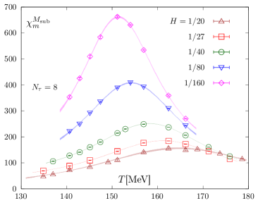
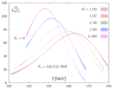
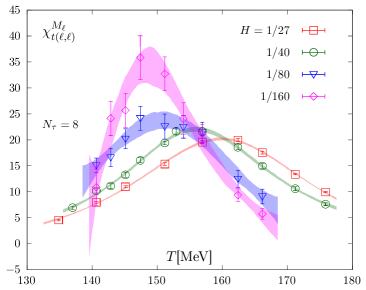
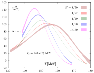
While the susceptibilities and are directly obtained from simulation data, the susceptibilities and are obtained by taking -derivatives of the rational polynomial ansätze used to fit and , respectively. As expected from Eqs. 29-30, we find that the rise of the maxima of the mixed susceptibilities with decreasing is slower than that of the chiral susceptibility .
We also calculate the mixed susceptibility , obtained by taking two derivatives of with respect to the strange quark chemical potential. This susceptibility first drops in the large quark mass region and starts to increase only for . It suggests that regular terms still contribute strongly to this susceptibility, which obviously is most sensitive to the strange quark sector. In our analysis of pseudo-critical temperatures we therefore do not include .
Pseudo-critical temperatures are obtained from maxima of the fit functions used to fit the susceptibilities. For and 444Note that we used in Eqs. 12 and 15, as a temperature independent normalization for the dimensionless mixed susceptibilities and . This insures that the maxima of these mixed susceptibilities agree with the inflection points of the order parameters and , respectively. , we use the maxima of the -derivative of the rational polynomial functions used to fit and respectively. The data for and have been interpolated directly using rational polynomial ansatze from which the maxima have been calculated. We use [3,2] Pade polynomials for all of the above fits. The error bands have been obtained from a bootstrap analysis. We summarize results of these fits in Table 3 and Fig. 5. Note that in the table as well as in the figure, we also include results for yet another mixed susceptibility obtained from a derivative of with respect to the strange quark mass. We discuss this observable in more detail in Section VI.
In the case of the mixed susceptibility obtained from we actually use three different observables, obtained by taking derivatives of the order parameter with respect to , the chemical potential or the strange quark mass (see Section VI for a discussion of the latter). In the scaling regime all these observables define the pseudo-critical temperature . In fact, as can be seen in Fig. 5 the location of maxima of these mixed susceptibilities is identical within errors even for the physical value of the light to strange quark mass ratio, . In addition to the mixed susceptibility , defined as the -derivative of , we also use the mixed susceptibility , which is obtained as the -derivative of the renormalized order parameter . This defines another pseudo-critical temperature, .
As can be seen in Fig. 5 the pseudo-critical temperatures reflect the ordering of the universal scaling relations for all . The pseudo-critical temperatures, however, are generally located outside the temperature range in which we found good scaling behavior for the order parameter , shown in Fig. 2. When fitting data for the pseudo-critical temperatures to extract we thus need to take into account also the influence of sub-leading corrections to the location of the maxima in susceptibilities.
We have fitted the data shown in Fig. 5 using scaling ansätze appropriate for the different observables used to define a pseudo-critical temperature and allowing for contributions from corrections-to-scaling as well as regular terms. We start with an ansatz for the unrenormalized order parameter ,
| (40) | |||||
and similarly for the renormalized order parameter , where gets replaced by . The definition of the corrections-to-scaling function and further details about the above ansatz are provided in Appendix B. Calculating the various susceptibilities by starting from Eq. 40 one obtains the influence of the sub-leading terms on the locations of the maxima of the susceptibilities by expanding the order parameter ansatz for small values of Bazavov et al. (2012) in the vicinity of the relevant, universal peak locations , or . Keeping terms up to for the determination of and for the determination of , , insures that in both cases regular terms linear in are kept in the determination of maxima of the susceptibilites. This gives for the position of a peak in the mixed susceptibilities
| (41) | |||||
whereas for the chiral susceptibility one has Bazavov et al. (2012),
The coefficient of the leading -dependent correction to is related to the universal parameters , given in Eqs. 31-33, and the non-universal scale ,
| (43) |
We performed fits in which and are kept as free fit parameters as well as using for and the values determined from the scaling fits to the order parameter given in Eqs. 36, 37. Using and as free fit parameters gives result that are consistent with Eqs. 36, 37.
We performed joint fits to data for pseudo-critical temperatures obtained from five different susceptibilities, demanding that they yield the same critical temperature in the chiral limit. It turns out that in the case of the mixed susceptibility these fits are not sensitive to a term proportional to . We thus set in our final fits. Furthermore, we need to control the influence of the smaller volume used in our determination of in calculations with . We therefore performed fits (i) leaving out or (ii) including the data for as well as (iii) using the data for where we corrected the values, obtained for , by a global shift of MeV. This is in accordance with the finite volume dependence found in Ding et al. (2019). For , it was found there that pseudo-critical temperatures determined at and differ by about MeV. We use this value also as an estimate for finite volume effects in our data obtained for at .
We find that fits using these three different approaches yield similar results for the chiral transition temperature ,
| (44) |
The resulting critical temperatures, extracted from the fits to pseudo-critical temperatures, thus are in good agreement with that determined from the scaling fit to the order parameter . We also find that keeping the slope parameters as free fit parameters gives results that are consistent with those obtained by fixing these coefficients to the universal values given in Eq. 43.
For our final fits we then fixed and using for the values given in Eqs. 36, 37 and the universal parameters , , , given in Eqs. 31-33. Our final joint fit of all data sets shown in Fig. 5 thus only depends on fit parameters fixing contributions from regular and correction-to-scaling terms.
The fit result, obtained by leaving out data obtained for , is shown in Fig. 5. This fit has a . The contribution arising only from the universal part of this fit, , is shown by dashed lines in Fig. 5. As can be seen this universal part dominates the fit of pseudo-critical temperatures, obtained from the mixed susceptibility , at least for . In the case of or , however, contributions from sub-leading corrections become important already for . This is in accordance with the conclusion drawn from the scaling fit performed for the order parameter , i.e. sub-leading corrections need to be taken into account for temperatures larger than .
V Curvature coefficients and pseudo-critical temperatures at
We have introduced the dependence of pseudo-critical temperatures on light and strange quark chemical potentials in Eq. 34. Equivalently this can be written in the basis where the chemical potentials and are obtained from those in the flavor basis using
| (45) |
With this we may rewrite Eq. 34 as,
| (46) | |||||
where the curvature coefficients calculated for vanishing chemical potentials using the quark-flavor or conserved charge basis, respectively, are related to each other through,
| (48) | |||||
We also note that the mixed curvature coefficients and carry quite different information. While the former is non-zero only due to flavor correlations arising, for instance, in high temperature perturbation theory only at Blaizot et al. (2001), the latter receives contributions also from diagonal terms in the strangeness sector.
The pseudo-critical temperatures in the basis (Eq. 46) may be re-written when imposing constraints on the strangeness chemical potential, e.g. in the case of a strangeness neutral medium. To leading order the strangeness chemical potential, insuring vanishing net strangeness number in an isospin symmetric medium is given by Bazavov et al. (2017), with . With this we obtain for the -dependence of pseudo-critical temperatures in strangeness-neutral, isospin-symmetric () matter,
| (50) | |||||
A recent calculation of for physical values of the light and strange quark masses is given in Bollweg et al. (2021). This yields . In Appendix A we present results for the dependence of on the quark mass ratio . An extrapolation to the chiral limit yields .
A calculation of curvature coefficients making use of the universal scaling relations discussed in the previous section has been performed previously at physical values of the quark masses Kaczmarek et al. (2011). Most calculations, however, make use of Taylor expansions for the dependence of the maximum of the chiral susceptibility or inflection points of the chiral condensates. In that case one starts from either Taylor expansions of the observables Kaczmarek et al. (2011); Bazavov et al. (2019); Bonati et al. (2018) or simulations performed with imaginary values of chemical potentials Bonati et al. (2015); Bellwied et al. (2015); Borsanyi et al. (2020),
Here and denotes the pseudo-critical temperature, which at non-vanishing values of light quark masses depends on the particular observable used for its definition. As discussed in the previous section, in the chiral limit all these pseudo-critical temperatures will converge to the uniquely defined phase transition temperature also for non-vanishing chemical potentials.
V.1 Curvature coefficients from the order parameter
Although the curvature coefficients are defined at , we may evaluate the relevant observables at any value of the temperature and for . Making use of the fact that derivatives of the order parameter with respect to energy-like couplings, i.e. temperature or chemical potentials, will be dominated by the diverging singular contribution, and using the Taylor expansion of the energy-like scaling field , we determine the curvature coefficient from a ratio of derivatives of order parameter with respect to chemical potentials and temperature, respectively,
| (52) | |||||
| (53) |
The curvature coefficients are then given by
| (54) | |||||
| (55) |
In the vicinity of the critical point at and for small values of the chemical potentials we may use the scaling ansatz for the order parameter , given in Eq.-27, to determine the curvature coefficients in the flavor basis. We will also take into account possible regular contributions to the order parameter using a linear ansatz similar to Eq.-40,
| (56) | |||||
Using the expansion of for small , i.e. in the vicinity of
| (57) | |||||
we may expand in the vicinity of ,
where the last line of Eq. V.1 gives explicitly the leading quark mass and temperature dependence arising from the rescaled regular term. Similar relations hold for the flavor off-diagonal curvature term . Furthermore, we may directly calculate ratios of curvature coefficients, e.g.
| (59) | |||||
We note that the scaling function as well as the critical exponents entering the scaling relations, of course, are specific to a given universality class. However, the basic definition of the curvature coefficients, given in Eqs. 52 and 53 as well as Eq. 59, do neither depend on the value of these exponents nor do they depend on the specific form of the scaling functions. The fact, that the global symmetry group for staggered fermions, used in our calculations at finite lattice spacings, is different from that of QCD in the continuum limit thus does not enter in these relations.
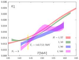
Results for and are shown in Fig. 6. From this we determine the curvature coefficients in flavor-basis at . It is apparent from Fig. 6 that the curvature coefficient related to the light quark chemical potential is almost an order of magnitude larger than that in the direction of the strange quark chemical potential. The off-diagonal curvature coefficient, in turn, is an order of magnitude smaller than . We give results for the various curvature coefficients and different quark mass ratios in Table-4.
| 1/27 | 0.109(2) | 0.0141(2) | 0.0004(4) | 0.0138(2) | -0.0048(1) | 0.147(1) |
| 1/40 | 0.111(2) | 0.0136(2) | 0.0009(5) | 0.0141(3) | -0.0048(2) | 0.129(1) |
| 1/80 | 0.121(7) | 0.0129(5) | 0.002(1) | 0.015(1) | -0.0052(5) | 0.111(2) |
| 1/160 | 0.12(1) | 0.0123(6) | 0.003(3) | 0.015(2) | -0.0048(10) | 0.098(2) |
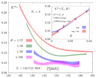
| 0 | 0.122(7) | 0.0124(5) | 0.003(2) | 0.015(1) | -0.0050(7) | 0.097(2) |
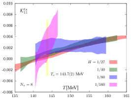
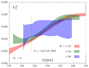
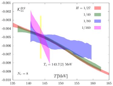
The resulting curvature coefficients in the () basis can be obtained by using similar equations corresponding to Eqs. 52 and 53. The curvature coefficients and are shown in Fig. 7. Note that is shown already in Fig. 6. Moreover, it is evident from Fig. 7 that the off-diagonal coefficient is clearly non-zero and negative. As expected, its value is dominated by the contribution of the diagonal curvature coefficient .
We fitted the results for curvature coefficients in the flavor basis, (, , ), as well as in the conserved charge basis, (, ) using for the quark mass dependence the ansatz given in Eq. V.1. Results of these fits are given in the last row of Table 4.
With this we find for the curvature coefficient in the case of (i) vanishing strangeness chemical potential, , (ii) along the strangeness neutral line, , and (iii) for vanishing strange quark chemical potential, ,
| (60) | |||||
| (61) | |||||
| (62) |
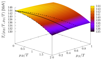
We thus find that the curvature coefficient in strangeness neutral matter is about 10% smaller than that for . In the curvature coefficient for the case , which corresponds to the relation and which sometimes is used as convenient approximation for the strangeness neutral case, is only about 3% smaller than . The above results for the curvature coefficients are reflected in the critical temperature surface in the - plane shown in Fig. 8. In that figure a solid line is shown for the case that corresponds to the strangeness neutral line in the - plane and two dashed lines show lines for constant and , respectively.
The results obtained here agree within errors with determinations of curvature coefficients obtained with physical light and strange quark masses and various choices for the chemical potentials (for recent summaries see e.g. D’Elia (2019); Borsanyi et al. (2020)). By making use of relations between curvature coefficients in the and ( basis, respectively, we could establish the systematic differences of curvature coefficients obtained along different lines of fixed .
VI Dependence of the chiral transition temperature on the strange quark mass
The dependence of the chiral phase transition temperature on chemical potentials, determined in the previous section to leading order in the chemical potentials, has been performed at fixed value of the strange quark mass. This has been tuned to its physical value . We may also use the various observables, obtained in the course of this analysis, to calculate the dependence of the chiral phase transition temperature on the value of the strange quark mass.
Varying the strange quark mass from to at vanishing values of the two degenerate light quark masses interpolates between the chiral limits of 3 and 2-flavor QCD, respectively. Several lattice QCD calculations, using different discretization schemes, suggest that the chiral phase transition in both limits remains to be second order. In particular, no indication for a first order transition in 3-flavor QCD has been found. We thus expect that universal features of the chiral phase transition in (2+1)-flavor QCD is described by the same universality class for all finite, non-zero values of the strange quark mass. As the strange quark mass does not break chiral symmetry in the light quark sector explicitly, it will appear as an external parameter in the energy-like scaling variable , just like the chemical potentials.
We may expand the chiral phase transition temperature , appearing in the definition of the energy-like scaling field given in Eq. 19, in terms of a Taylor series around the physical strange mass, . To leading order we obtain,
| (63) | |||||
Omitting just for clarity the -dependence of the scaling variable , introduced in Eq. 19, we rewrite as
where
| (66) |
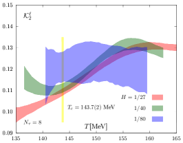
Using the definition of the light-strange susceptibility, introduced in Eq. 11, we may obtain the curvature coefficient from the ratio
| (67) |
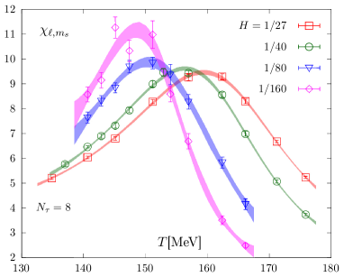
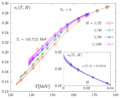
Results for the light-strange susceptibility are shown in Fig. 9 (top). We see that the peak position of the susceptibility shifts to smaller values as decreases. Results for the pseudo-critical temperatures corresponding to the location of these peaks are also given in Table 3 and shown in Fig. 5. It is apparent that these pseudo-critical temperatures vary with just like the other mixed susceptibilities obtained from derivatives of the chiral order parameter with respect to a energy-like variable. This confirms our expectation that that the strange quark mass enters the universal scaling relations just like other energy-like couplings.
Results for , obtained for several values of , are shown in Fig. 9 (bottom). From this we obtain the curvature coefficient in the chiral limit as
| (68) |
From a fit to the data for , using only the leading correction arising from a regular term (reg) proportional to as well as the additional sub-leading correction arising from a correction-to-scaling (cts) contribution,
| (69) |
we obtain
| (70) |
where the errors include the uncertainty on . It is interesting to note here that the cts term is parametrically sub-leading relative to the regular term in contrast to the case for pseudo-critical temperatures in Eqs. 41 and IV.2 (see Appendix B for more details). Establishing the importance of corrections-to-scaling terms would require a more detailed analysis of the -dependence of at small values of . From both extrapolations shown in the inset of Fig. 9 we conclude that the variation of the chiral phase transition temperature with the strange quark mass is rather small. A variation of by 10% would lead to a change of by less than 1%.
VII Conclusions
We have performed a systematic analysis of the light quark mass dependence of pseudo-critical temperatures in (2+1)-flavor QCD with the strange quark mass tuned to its physical value. Making use of scaling relations that describe the dependence of the magnetic equation of state on energy-like scaling fields, i.e. temperature and chemical potentials, close to the chiral limit, we determined the leading order Taylor expansion coefficients (curvature coefficients) defining the dependence of the chiral phase transition temperature on the strangeness and baryon number chemical potentials, , for several values of the light to strange quark mass ratio , and extrapolated these curvature coefficients to the chiral limit (). We find that the curvature coefficient decreases on lines of constant with increasing . On a line corresponding to strangeness neutral matter () it is about 10% smaller in than on a line with vanishing strangeness chemical potential ().
The curvature coefficients on lines with fixed obtained on lattices with temporal extent at turn out to be consistent with the corresponding continuum extrapolated results obtained with the physical light to strange quark mass ratio, , at the pseudo-critical temperature MeV. In the latter case one has with Bazavov et al. (2019), 0.0145(25) Bonati et al. (2018), 0.0153(18) Borsanyi et al. (2020), whereas in the chiral limit we obtain the not yet continuum extrapolated result .
Acknowledgments
This work was supported by the Deutsche Forschungsgemeinschaft (DFG, German Research Foundation) Proj. No. 315477589-TRR 211; and the PUNCH4NFDI consortium supported by the Deutsche Forschungsgemeinschaft (DFG, German Research Foundation) with project number 460248186 (PUNCH4NFDI). It also has been supported in part by the Taiwanese NSTC project 112-2639-M-002-006-ASP; the National Natural Science Foundation of China under Grant No. 12325508 and the National Key Research and Development Program of China under Contract No. 2022YFA1604900; the U.S. Department of Energy, Office of Science, Office of Nuclear Physics through Contract No. DE-SC0012704, and within the frameworks of Scientific Discovery through Advanced Computing (SciDAC) award Fundamental Nuclear Physics at the Exascale and Beyond as well as by the U.S. National Science Foundation under award PHY-2309946.
Numerical calculations have been made possible through PRACE grants at CSCS, Switzerland. Additional calculations have been performed on the GPU clusters at Bielefeld University, Germany, the Central China Normal University, China, and using USQCD resources at the Thomas Jefferson National Accelerator Facility, USA.
We also acknowledge very helpful discussions with Anirban Lahiri and his valuable contributions to the early stages of this work.
Appendix A Strangeness neutrality in the chiral limit
We give here results for the quark mass dependence of the leading order strangeness neutrality relation between the strangeness and baryon number chemical potentials.
Expanding the net strangeness number density, , to leading order in the chemical potentials gives,
| (71) |
where , with , and are second order conserved charge cumulants. Their definition and recent continuum extrapolated results obtained in calculations with the HISQ action are given in Bollweg et al. (2021). In the case of vanishing electric charge chemical potential, , which is considered throughout this work, one thus finds from Eq. 71 that strangeness and baryon number chemical potentials are related through,
| (72) |
with
| (73) |
Continuum extrapolated results for this ratio at physical values of the light and strange quark masses, i.e. for have also been reported in Bollweg et al. (2021)
| (74) |
Here is obtained by averaging over continuum extrapolated results for and Bazavov et al. (2019). For the analysis presented in this work we are interested in the chiral limit results at the chiral phase transition temperature on lattices with fixed , i.e., we want to determine . In Fig. 10 we show results for obtained on lattices with temporal extent as function of temperature and quark mass ratio . In the inset of Fig. 10 we show . A chiral extrapolation of these data, using the scaling ansatz appropriate for the scaling of energy-like observables in the , universality classes Clarke et al. (2021),
| (75) |
yields
| (76) |
where the error includes the statistical error and the uncertainty arising from the error on . In order to provide further support for the use of a scaling ansatz for the chiral extrapolation, clearly more data at different values of are needed.
Appendix B Corrections-to-Scaling and regular contributions
The leading singular contribution to the free energy density has been introduced in Eq. 22. Sub-dominant, still divergent, universal corrections to this arise from from another scaling field, in the singular part of the free energy density,
| (77) |
with , with , .
This can be used as a starting point for a scaling analysis that takes into account corrections to scaling. The magnetization then is given by
| (78) | |||||
Here and denote the derivatives of with respect to the first and second argument, respectively.
For small , i.e. close to the chiral limit, one may expand in terms of . Keeping only the leading order correction term one gets,
| (79) |
where has been introduced in Eq. 25 and .
In addition to the correction-to-scaling (cts) term we also consider a contribution from regular terms,
| (80) | |||||
From this one obtains for the mixed susceptibility ,
| (81) | |||||
In the absence of contributions from regular and cts terms, has a maximum at a pseudo-critical temperature given by the condition . Corrections to this result will be small for small . We therefore expand the right hand side of Eq. 81 around the maximum of , i.e. around ,
| (82) | |||||
With this we determine the location of the maximum of ,
| (83) | |||||
Similarly one finds for the pseudo-critical temperature , determined from the maximum of , Bazavov et al. (2012)
| (84) | |||||
Note that regular contributions are suppressed relative to the corrections-to-scaling terms in and .
The curvature coefficients are obtained from ratios of susceptibilities, e.g. like given in Eq. V.1. These ratios will be evaluated at or close to . In the presence of corrections-to-scaling the scaling function , appearing in that equation, gets replaced by . The cts term thus multiplies the dominant divergent term and is proportional to the curvature coefficient, e.g. .
At one obtains
| (85) |
with . In the absence of a regular term the cts contribution thus cancels and there is no -dependent correction to . As a consequence the cts corrections becomes sub-leading to the regular term, i.e.
| (86) | |||||
References
- Bazavov et al. (2019) A. Bazavov et al. (HotQCD), Phys. Lett. B 795, 15 (2019), arXiv:1812.08235 [hep-lat] .
- Bhattacharya et al. (2014) T. Bhattacharya et al., Phys. Rev. Lett. 113, 082001 (2014), arXiv:1402.5175 [hep-lat] .
- Borsanyi et al. (2020) S. Borsanyi, Z. Fodor, J. N. Guenther, R. Kara, S. D. Katz, P. Parotto, A. Pasztor, C. Ratti, and K. K. Szabo, Phys. Rev. Lett. 125, 052001 (2020), arXiv:2002.02821 [hep-lat] .
- Ding et al. (2019) H. Ding et al., Phys. Rev. Lett. 123, 062002 (2019), arXiv:1903.04801 [hep-lat] .
- Kotov et al. (2021) A. Y. Kotov, M. P. Lombardo, and A. Trunin, Phys. Lett. B 823, 136749 (2021), arXiv:2105.09842 [hep-lat] .
- Braun et al. (2023) J. Braun et al., (2023), arXiv:2310.19853 [hep-ph] .
- Cuteri et al. (2021) F. Cuteri, O. Philipsen, and A. Sciarra, JHEP 11, 141 (2021), arXiv:2107.12739 [hep-lat] .
- Halasz et al. (1998) A. M. Halasz, A. D. Jackson, R. E. Shrock, M. A. Stephanov, and J. J. M. Verbaarschot, Phys. Rev. D 58, 096007 (1998), arXiv:hep-ph/9804290 .
- Hatta and Ikeda (2003) Y. Hatta and T. Ikeda, Phys. Rev. D 67, 014028 (2003), arXiv:hep-ph/0210284 .
- Stephanov (2006) M. A. Stephanov, Phys. Rev. D 73, 094508 (2006), arXiv:hep-lat/0603014 .
- Buballa and Carignano (2019) M. Buballa and S. Carignano, Phys. Lett. B 791, 361 (2019), arXiv:1809.10066 [hep-ph] .
- Pisarski and Wilczek (1984) R. D. Pisarski and F. Wilczek, Phys. Rev. D 29, 338 (1984).
- Butti et al. (2003) A. Butti, A. Pelissetto, and E. Vicari, JHEP 08, 029 (2003), arXiv:hep-ph/0307036 .
- Buchoff et al. (2014) M. I. Buchoff et al., Phys. Rev. D 89, 054514 (2014), arXiv:1309.4149 [hep-lat] .
- Pelissetto and Vicari (2013) A. Pelissetto and E. Vicari, Phys. Rev. D 88, 105018 (2013), arXiv:1309.5446 [hep-lat] .
- Resch et al. (2019) S. Resch, F. Rennecke, and B.-J. Schaefer, Phys. Rev. D 99, 076005 (2019), arXiv:1712.07961 [hep-ph] .
- Aoki et al. (2021) S. Aoki, Y. Aoki, G. Cossu, H. Fukaya, S. Hashimoto, T. Kaneko, C. Rohrhofer, and K. Suzuki (JLQCD), Phys. Rev. D 103, 074506 (2021), arXiv:2011.01499 [hep-lat] .
- Ding et al. (2021) H. T. Ding, S. T. Li, S. Mukherjee, A. Tomiya, X. D. Wang, and Y. Zhang, Phys. Rev. Lett. 126, 082001 (2021), arXiv:2010.14836 [hep-lat] .
- Ding et al. (2023) H.-T. Ding, W.-P. Huang, S. Mukherjee, and P. Petreczky, Phys. Rev. Lett. 131, 161903 (2023), arXiv:2305.10916 [hep-lat] .
- Kovacs (2023) T. G. Kovacs, (2023), arXiv:2311.04208 [hep-lat] .
- Karsch (2019) F. Karsch, PoS CORFU2018, 163 (2019), arXiv:1905.03936 [hep-lat] .
- Allton et al. (2002) C. R. Allton, S. Ejiri, S. J. Hands, O. Kaczmarek, F. Karsch, E. Laermann, C. Schmidt, and L. Scorzato, Phys. Rev. D 66, 074507 (2002), arXiv:hep-lat/0204010 .
- Kaczmarek et al. (2011) O. Kaczmarek, F. Karsch, E. Laermann, C. Miao, S. Mukherjee, P. Petreczky, C. Schmidt, W. Soeldner, and W. Unger, Phys. Rev. D 83, 014504 (2011), arXiv:1011.3130 [hep-lat] .
- Bonati et al. (2015) C. Bonati, M. D’Elia, M. Mariti, M. Mesiti, F. Negro, and F. Sanfilippo, Phys. Rev. D 92, 054503 (2015), arXiv:1507.03571 [hep-lat] .
- Bellwied et al. (2015) R. Bellwied, S. Borsanyi, Z. Fodor, J. Günther, S. D. Katz, C. Ratti, and K. K. Szabo, Phys. Lett. B 751, 559 (2015), arXiv:1507.07510 [hep-lat] .
- Cea et al. (2016) P. Cea, L. Cosmai, and A. Papa, Phys. Rev. D 93, 014507 (2016), arXiv:1508.07599 [hep-lat] .
- Bonati et al. (2018) C. Bonati, M. D’Elia, F. Negro, F. Sanfilippo, and K. Zambello, Phys. Rev. D 98, 054510 (2018), arXiv:1805.02960 [hep-lat] .
- D’Elia (2019) M. D’Elia, Nucl. Phys. A 982, 99 (2019), arXiv:1809.10660 [hep-lat] .
- Biswas et al. (2024) D. Biswas, P. Petreczky, and S. Sharma, (2024), arXiv:2401.02874 [hep-ph] .
- Clarke et al. (2021) D. A. Clarke, O. Kaczmarek, F. Karsch, A. Lahiri, and M. Sarkar, Phys. Rev. D 103, L011501 (2021), arXiv:2008.11678 [hep-lat] .
- Kaczmarek et al. (2022) O. Kaczmarek, F. Karsch, A. Lahiri, S.-T. Li, M. Sarkar, C. Schmidt, and P. Scior, PoS LATTICE2021, 429 (2022), arXiv:2112.15398 [hep-lat] .
- Follana et al. (2007) E. Follana, Q. Mason, C. Davies, K. Hornbostel, G. P. Lepage, J. Shigemitsu, H. Trottier, and K. Wong (HPQCD, UKQCD), Phys. Rev. D 75, 054502 (2007), arXiv:hep-lat/0610092 .
- Bazavov et al. (2012) A. Bazavov et al., Phys. Rev. D 85, 054503 (2012), arXiv:1111.1710 [hep-lat] .
- Bollweg et al. (2021) D. Bollweg, J. Goswami, O. Kaczmarek, F. Karsch, S. Mukherjee, P. Petreczky, C. Schmidt, and P. Scior (HotQCD), Phys. Rev. D 104 (2021), 10.1103/PhysRevD.104.074512, arXiv:2107.10011 [hep-lat] .
- Aoki et al. (2020) S. Aoki et al. (Flavour Lattice Averaging Group), Eur. Phys. J. C 80, 113 (2020), arXiv:1902.08191 [hep-lat] .
- Bollweg et al. (2022) D. Bollweg, L. Altenkort, D. A. Clarke, O. Kaczmarek, L. Mazur, C. Schmidt, P. Scior, and H.-T. Shu, PoS LATTICE2021, 196 (2022), arXiv:2111.10354 [hep-lat] .
- Mazur et al. (2023) L. Mazur et al. (HotQCD), (2023), arXiv:2306.01098 [hep-lat] .
- Gavai and Gupta (2003) R. V. Gavai and S. Gupta, Phys. Rev. D 68, 034506 (2003), arXiv:hep-lat/0303013 .
- Allton et al. (2005) C. R. Allton, M. Doring, S. Ejiri, S. J. Hands, O. Kaczmarek, F. Karsch, E. Laermann, and K. Redlich, Phys. Rev. D 71, 054508 (2005), arXiv:hep-lat/0501030 .
- Cheng et al. (2008) M. Cheng et al., Phys. Rev. D 77, 014511 (2008), arXiv:0710.0354 [hep-lat] .
- Ejiri et al. (2009) S. Ejiri, F. Karsch, E. Laermann, C. Miao, S. Mukherjee, P. Petreczky, C. Schmidt, W. Soeldner, and W. Unger, Phys. Rev. D 80, 094505 (2009), arXiv:0909.5122 [hep-lat] .
- Engels et al. (2000) J. Engels, S. Holtmann, T. Mendes, and T. Schulze, Phys. Lett. B 492, 219 (2000), arXiv:hep-lat/0006023 .
- Hasenbusch and Toeroek (1999) M. Hasenbusch and T. Toeroek, J. Phys. A 32, 6361 (1999), arXiv:cond-mat/9904408 .
- Karsch et al. (2023) F. Karsch, M. Neumann, and M. Sarkar, Phys. Rev. D 108, 014505 (2023), arXiv:2304.01710 [hep-lat] .
- Blaizot et al. (2001) J. P. Blaizot, E. Iancu, and A. Rebhan, Phys. Lett. B 523, 143 (2001), arXiv:hep-ph/0110369 .
- Bazavov et al. (2017) A. Bazavov et al., Phys. Rev. D 95, 054504 (2017), arXiv:1701.04325 [hep-lat] .