Gravitational Waves in Chern-Simons-Gauss-Bonnet Gravity

Abstract

It is known that the four-dimensional effective field theory arising from heterotic string theory is general relativity with both a Chern-Simons and Gauss-Bonnet term. We study the propagation of gravitational waves in this combination of Chern-Simons and Gauss-Bonnet gravity, both of which have an associated scalar field, the axion and the dilaton respectively, that are kinetically coupled. We review how the combination of dynamical Chern-Simons and Gauss-Bonnet gravities can arise from string theory as corrections to general relativity and show how the gravitational wave waveform is modified in such a theory. We compare our results to a novel framework recently introduced for parametrizing the parity-violating sector (Chern-Simons), and use that to guide our construction of a similar parametrization for the parity-conserving (Gauss-Bonnet) sector. In general, we find that the contributions from the parity-violating and parity-conserving sectors are similar. Moreover, the kinetic coupling between the axion and dilaton introduces an extra contribution to the parity-violating sector of the gravitational waves. Using our parametrization, we are able to comment on initial constraints for the theory parameters, including the time variations of the axion and dilaton.

I Introduction

Einstein’s theory of general relativity (GR) has been shown to agree remarkably well with observations Abbott et al. (2019a, b, 2021a); Collaboration et al. (2021). However, theoretical and observational challenges suggest that GR may be modified in the strong field regime Will (2014). These corrections are generally motivated from a high-energy ultraviolet (UV) theory that, at low energies, leads to corrections to GR in an effective field theory (EFT).

GR has been very well constrained in the weak field regime (see e.g. Shapiro (1990); S. and M.-T. (2009)), and with the ability to detect gravitational waves (GWs) in the last decade, it has become possible to probe the strong field regime of gravity directly using compact objects, such as black holes and neutron stars Abbott et al. (2019c, 2021b, 2023, 2017). Thus, GWs have opened up a new avenue for testing potential modifications of GR.

There are a wide range of modified gravity theories and extensions to GR (see e.g. Capozziello and De Laurentis (2011); Faraoni and Capozziello (2011) for a review), which may be motivated from the fact that, at high energies, GR is non-renormalizable in a quantum theory of gravity. Modifications to GR have also been proposed as alternatives to inflation, dark matter, and dark energy (e.g., Faraoni and Capozziello (2011); Nojiri and Odintsov (2007); Nojiri et al. (2017)). Modified gravity theories are either parity-conserving, which remain invariant under a parity transformation, or parity-violating, which are not invariant under such a transformation.

Many well-studied modifications to GR incorporate higher curvature terms. Some well-studied parity-conserving theories are Gauss-Bonnet Boulware and Deser (1986); Kanti et al. (1996); Torii et al. (1997); Alexeyev and Pomazanov (1997) and Starobinsky inflation as a specific type of $f(R)$ gravity Starobinsky (1980); Sotiriou and Faraoni (2010). Examples of parity-violating theories include Chern-Simons gravity Lue et al. (1999); Jackiw and Pi (2003); Alexander and Yunes (2009); Yunes and Pretorius (2009a), parity violating extensions to Teleparallel Gravity Crisostomi et al. (2018); Conroy and Koivisto (2019), Horava-Lifshitz Hořava (2009); Zhu et al. (2013), and ghost-free scalar-tensor gravity Nishizawa and Kobayashi (2018). Recent work has also shown that parity-violating gravitational interactions can be constructed from the Kalb-Ramond field Manton and Alexander (2024).

Two well-studied modified gravity theories are Chern-Simons and Gauss Bonnet gravity. Chern-Simons gravity can be motivated from the context of particle physics Alvarez-Gaume and Witten (1984); Weinberg (2013) and leptogenesis Alexander et al. (2006); Alexander and Gates (2006), as well as in other areas such as string theory Green and Schwarz (1984, 1985); Green et al. (1988a), loop quantum gravity Ashtekar and Lewandowski (2004); Thiemann (2001); Rovelli (2004) and effective field theories Alexander et al. (2021); Alexander and Creque-Sarbinowski (2023). Furthermore, from a phenomenological perspective, such a theory could give rise to parity violation in the cosmic microwave background (CMB) Wu et al. (2009); Sorbo (2011); Shiraishi et al. (2013); Shiraishi (2016); Philcox (2023) and in the gravitational sector Lue et al. (1999); Jackiw and Pi (2003); Contaldi et al. (2008); Alexander and Yunes (2018); Loutrel and Yunes (2022). Notably, parity violation in the gravitational sector can lead to birefringence in GW propagation, in which the right- and left- handed polarization modes evolve differently in their amplitude and/or velocity.

Gauss-Bonnet gravity is another well-motivated modified gravity theory, initially arising from an attempt to generalize GR Lanczos (1932, 1938); Lovelock (1970, 1971); it has also been suggested to arise from string theory Zwiebach (1985); Gross and Sloan (1987); Nepomechie (1985); Callan et al. (1986); Candelas et al. (1985). Its phenomenological implications have been extensively studied, including its predicted effect on compact objects such as black holes and neutron stars Moura and Schiappa (2006); Guo et al. (2008); Maeda et al. (2009); Pani and Cardoso (2009); Kleihaus et al. (2011); Ayzenberg and Yunes (2014); Maselli et al. (2015); Kleihaus et al. (2016); Kokkotas et al. (2017), and its implications for inflation Kanti et al. (2015); Chakraborty et al. (2018); Odintsov and Oikonomou (2018); Yi and Gong (2019); Odintsov and Oikonomou (2019); Rashidi and Nozari (2020).

One avenue to find modifications to GR that are mathematically well-motivated is string theory, a candidate for a quantum theory of gravity and a unified description of the fundamental forces of Nature Green et al. (1988b, a); Polchinski (2007a, b, 1994). In general, constructions of string theory require more than four dimensions. Upon compactification from a higher-dimensional theory to four dimensions, string theory predicts GR plus perturbative corrections in the string tension $\alpha^{\prime}=\ell_{s}^{2}$ Callan et al. (1985); Gross and Sloan (1987); Hull and Townsend (1987); Metsaev and Tseytlin (1987), and some of these corrections are quadratic curvature terms Zwiebach (1985); Deser and Redlich (1986). In general, corrections to the Einstein-Hilbert action are represented locally by higher derivative additions, and coordinate invariance implies that they must consist of second and higher powers of curvatures, and their derivatives Deser and Tekin (2002).

A natural question to ask then, is what would be precisely the effective four-dimensional gravity theory predicted from string theory. In string theory, the heterotic string is a mixture of the right-moving sector of the superstring and the left-moving sector of the bosonic string. The two sectors need different spacetime dimensions to cancel the anomalies; the matching of dimensions is achieved by compactifying the extra dimensions on a compact manifold. Heterotic string theory (HST) possesses a number of attractive features, including that it is chiral and includes gauge fields Gross et al. (1985, 1986). The two possible gauge groups for the heterotic string are $E_{8}\times E_{8}$ and $SO(32)$ Gross et al. (1985); furthermore, the superstring’s spectrum contains no tachyons and has a graviton Blumenhagen et al. (2013).

For a long time, it has been theorized that the four-dimensional effective action from HST is captured by GR plus a Gauss-Bonnet term. However, this lacks an axion field; the field strength of the Kalb-Ramond 2-form satisfies the Bianchi identity $dH=\alpha^{\prime}R\wedge R$, and hence this term cannot be truncated out. Upon compactification to four dimensions, this term results in a correction to GR that can be precisely identified as the Pontryagin term of Chern-Simons gravity, which is typically coupled to an axion field. Thus, for HST, the 4D gravity theory cannot be Gauss-Bonnet or Chern-Simons gravities alone, but rather a combination of the two as corrections to GR, a result that does not depend on the choice of compactification Cano and Ruipérez (2022).

GWs are a powerful probe of modified gravity theories. It is well known that the effects of deviations from GR on GWs can generally be characterized by modifications to the GW amplitude and phase, for example by using the parametrized post-Einsteinian formalism (ppE) Yunes and Pretorius (2009b); Mirshekari et al. (2012); Yunes and Siemens (2013); Yunes et al. (2016); Tahura and Yagi (2018); Tahura et al. (2019); Ezquiaga et al. (2021, 2022). In this paper, we study Chern-Simons-Gauss-Bonnet (CS-GB) gravity by computing the equations of motion of GW propagation for such a theory, which contains both terms and includes a kinetic coupling between the two associated scalar fields, the axion and the dilaton. We map our analytic expressions to the parity-violating framework put forth in Jenks et al. (2023) and provide an explicit extension to the parity-invariant sector. This extension maps to ppE and provides a framework to explicitly parameterize parity-violating and parity-conserving corrections to GR in GW propagation. From this framework and our mapping of the CS-GB parameters to GW observables, we are able to use the constraints on the GW propagation speed, as well as the coupling constant $\alpha^{\prime}$, to provide initial constraints on the theory.

The outline of this paper is as follows: after presenting the basics of CS and GB gravities in Section II, we review in Section III how both theories can arise from HST by summarizing the stringy derivation from Cano and Ruipérez (2022) of the 4D effective action, which showed that the result is a combination of CS and GB gravities. In Section IV we compute the modified field equations, and in Section V we calculate the equations of motion for GWs in an FLRW background. From there, we generalize the parametrization of Jenks et al. (2023) by including the parity-conserving sector, and use the full parametrization to place initial constraints on the CS-GB theory parameters, including the time derivatives of the axion and dilaton, in Section VI. We briefly discuss other effects, directions for future work, and conclude in Section VII.

Throughout this paper, we use geometric units such that $G=c=1$, and we assume a $(-,+,+,+)$ metric signature; Greek letters ($\mu$,$\nu$,…) range over all spacetime coordinates, Latin letters (i,j,…) range over spatial indices, and square brackets denote anti-symmetrization over indices.

II Basics of Chern-Simons and Gauss-Bonnet Gravities

In this section, we review the basics of Chern-Simons (Sec. II.1) and Gauss-Bonnet (Sec. II.2) gravities individually, before turning to the combined theory for the remainder of the paper.

II.1 Chern-Simons Gravity

The CS modification of GR arises in different contexts, including in particle physics Alvarez-Gaume and Witten (1984); Alexander and Creque-Sarbinowski (2023) and in string theory, where it arises from the Green-Schwarz anomaly cancellation mechanism Green and Schwarz (1984, 1985); Green et al. (1988a). In other words, in HST, a quantum effect due to a gauge field induces a CS term in the effective low energy 4D action of GR.

CS gravity is a 4D deformation of GR that can generally be written as

$$S=S_{\mbox{\tiny EH}}+S_{\mbox{\tiny CS}}+S_{\varphi}+S_{\text{mat}},$$ (1)

where $S_{\mbox{\tiny EH}}$ is the usual Einstein-Hilbert action of GR

$$S_{\mbox{\tiny EH}}=\int d^{4}x\sqrt{-g}R,$$ (2)

the CS term is given by

$$S_{\mbox{\tiny CS}}=\frac{\alpha}{4\kappa}\int d^{4}x\varphi^{*}RR,$$ (3)

with $\kappa=(16\pi)^{-1}$, and $\alpha$ is a coupling parameter. The pseudo-scalar field, $\varphi$, is coupled to the Pontryagin density of the spacetime, which is defined as

$${}^{*}RR=*R^{\mu}_{~{}\nu}{}^{\rho\sigma}R^{\nu}_{~{}\mu\rho\sigma},$$ (4)

where the Hodge dual of the Riemann tensor is

$$*R^{\mu}_{~{}\nu}{}^{\rho\sigma}=\frac{1}{2}\epsilon^{\rho\sigma\alpha\beta}R^{\mu}_{~{}\nu\alpha\beta},$$ (5)

with $\epsilon^{\rho\sigma\alpha\beta}$ the antisymmetric Levi-Civita tensor. The scalar field term is

$$S_{\varphi}=-\frac{\beta}{2}\int d^{4}x\sqrt{-g}[g^{\mu\nu}(\nabla_{\mu}\varphi)(\nabla_{\nu}\varphi)+2V(\varphi)],$$ (6)

and lastly we can have an additional matter contribution described by

$$S_{\text{mat}}=\int d^{4}x\sqrt{-g}\mathcal{L}_{\text{mat}},$$ (7)

where $\mathcal{L}_{\text{mat}}$ is a matter Lagrangian density that does not depend on $\varphi$.

If a nonzero potential $V(\varphi)$ is chosen in Eq. (6), then a mass for the scalar field usually has to be generated, which would render the field short-ranged. However, Eq. (1) has a shift symmetry, and theories with a shift symmetry do not allow mass terms, hence the field must be long-ranged. Thus, we choose to set $V(\varphi)$ = 0 and neglect the potential term.

The pseudo-scalar $\varphi$ is known as the CS coupling field, which can generically be a function of space and time. If $\varphi=constant$, CS gravity reduces to GR, since the Pontryagin term can be expressed as the divergence of the CS topological current $K_{\mu}$,

$$\nabla_{\mu}K^{\mu}=\frac{1}{2}{}^{*}RR,$$ (8)

where

$$K^{\mu}=\epsilon^{\mu\nu\rho\sigma}\Gamma^{n}_{\nu m}\bigg{(}\partial_{\rho}\Gamma^{m}_{\sigma n}+\frac{2}{3}\Gamma^{m}_{\rho l}\Gamma^{l}_{\sigma n}\bigg{)},$$ (9)

with $\Gamma$ being the Christoffel connection. Upon integration by parts, $S_{\mbox{\tiny CS}}$ becomes

$$S_{\mbox{\tiny CS}}=\alpha(\varphi K^{\mu})\biggr{\rvert}_{\partial\mathcal{V}}-\frac{\alpha}{2}\int_{\mathcal{V}}d^{4}x\sqrt{-g}(\nabla_{\mu}\varphi)K^{\mu},$$ (10)

and the first term can be discarded because it is evaluated on the boundary of the manifold, while the second term clearly vanishes if $\varphi$ is constant Alexander and Yunes (2009).

The addition of the CS terms modifies the Einstein equations by the addition of the C-tensor, $C_{\mu\nu}$, as

$$G_{\mu\nu}+\frac{\alpha}{\kappa}C_{\mu\nu}=\frac{1}{2\kappa}T_{\mu\nu}.$$ (11)

The C-tensor is a 4D generalization of the 3D Cotton-York tensor; it is given by

$$C^{\mu\nu}=(\nabla_{\alpha}\varphi)\epsilon^{\alpha\beta\gamma(\mu}\nabla_{\gamma}R^{\nu)}_{~{}\beta}+[\nabla_{(\alpha}\nabla_{\beta)}\varphi]~{}^{*}R^{\beta(\mu\nu)\alpha}.$$ (12)

Furthermore, we get an extra equation of motion for $\varphi$ from the variation of the action:

$$\beta\Box\varphi=-\frac{\alpha}{4}~{}^{*}RR,$$ (13)

which is the Klein-Gordon equation in the presence of a source term.

Here we note that there are two formulations of CS gravity (Eq. (1)): the non-dynamical formulation ($\alpha$ arbitrary, $\beta=0$) and the dynamical formulation ($\alpha$ and $\beta$ arbitrary but nonzero). These are two distinct theories, because in the dynamical case the scalar field introduces stress-energy into the field equations, which forces vacuum spacetimes to possess a certain amount of “scalar hair,” a feature which is absent in the non-dynamical formulation. In this paper, we will be considering the dynamical formulation of CS gravity, appropriately called dynamical Chern-Simons (dCS) gravity.

II.2 Gauss-Bonnet Gravity

Gauss-Bonnet gravity has been well studied and it has been found to exhibit a rich phenomenology (see e.g. Sotiriou and Zhou (2014a, b); Doneva and Yazadjiev (2018); Silva et al. (2018); Antoniou et al. (2018); Cunha et al. (2019)), from producing viable models of inflation to spontaneous scalarization in compact objects, as well as admitting novel black hole solutions that evade the no-hair theorems Herdeiro and Radu (2018). At the classical level, string theory predicts that Einstein’s field equations receive next-to-leading-order corrections that are usually described by higher-order curvature terms in the action. In particular, GB terms occur in HST in the 1-loop effective action of the 4D theory, in the Einstein frame Zwiebach (1985); Gross and Sloan (1987); Nepomechie (1985); Callan et al. (1986); Candelas et al. (1985).

The GB action is another deformation of GR that can be written as

$$S=S_{\mbox{\tiny EH}}+S_{\mbox{\tiny GB}},$$ (14)

with $S_{\mbox{\tiny EH}}$ given in Eq. (2) and

$$S_{\mbox{\tiny GB}}=\int d^{4}x\sqrt{-g}\bigg{[}-\frac{1}{2}\partial_{\alpha}\phi\partial^{\alpha}\phi+\alpha f(\phi)\mathcal{X}_{4}\bigg{]},$$ (15)

where $\alpha$ is a coupling constant, $\mathcal{X}_{4}$ is the 4D GB density,

$$\mathcal{X}_{4}=R^{2}-4R_{\mu\nu}R^{\mu\nu}+R_{\mu\nu\rho\sigma}R^{\mu\nu\rho\sigma},$$ (16)

and we have included a kinetic term for the scalar field.

A standard variation of Eq. (14) yields the field equations Bryant et al. (2021):

$$\Box\phi =\alpha f^{\prime}(\phi)\mathcal{X}_{4},$$ (17)

$$G_{\mu\nu} =\frac{1}{2}\partial_{\mu}\phi\partial_{\nu}\phi-\frac{1}{4}g_{\mu\nu}\partial_{\alpha}\phi\partial^{\alpha}\phi-\alpha D_{\mu\nu}^{(\phi)}+8\pi T_{\mu\nu},$$ (18)

where $G_{\mu\nu}$ is the Einstein tensor, $T_{\mu\nu}$ is the matter stress-energy tensor, and

$$D_{\mu\nu}^{(\phi)}=(g_{\mu\rho}g_{\nu\sigma}+g_{\mu\sigma}g_{\nu\rho})\epsilon^{\alpha\sigma\lambda\gamma}\nabla_{\kappa}[^{*}R^{\rho\kappa}_{~{}\lambda\gamma}\partial_{\alpha}f(\phi)].$$ (19)

For $D=4$, one can see that, when varying Eq. (14) with respect to the inverse metric, the contributions of the GB density to the field equations vanish identically. However, if there is a dynamical scalar field $\phi$ which is coupled to the GB density, the GB term will have non-vanishing contributions to the field equations, even in four dimensions. This scalar field $\phi$ is conventially referred to as the dilaton.

The combination of the Einstein-Hilbert and GB terms in the gravitational action is known as Einstein-Gauss-Bonnet gravity, and with the inclusion of the dilaton it is referred to as Einstein-dilaton-Gauss-Bonnet (EdGB) gravity, which is what we consider in this paper.

III Derivation of 4D Effective String Action

Here we review how CS-GB gravity can arise from HST, a result which was derived in Cano and Ruipérez (2022). We outline the most important steps in this section, with more intermediate steps and explanations provided in Appendix A.

Our starting point is the ten-dimensional heterotic superstring effective action at first order in $\alpha^{\prime}$. We will use the action given by Bergshoeff and de Roo (1989), which is obtained upon supersymmetrization of the Lorentz-Chern-Simons terms:

$$\hat{S} =\frac{g_{s}^{2}}{16\pi G_{N}^{(10)}}\int d^{10}x\sqrt{|\hat{g}|}e^{-2\hat{\phi}}\bigg{[}\hat{R}-4(\partial\hat{\phi})^{2}+\frac{1}{12}\hat{H}^{2}$$

$$+\frac{\alpha^{\prime}}{8}\hat{R}_{(-)\mu\nu ab}\hat{R}_{(-)}^{\mu\nu ab}+\mathcal{O}(\alpha^{\prime 3})\bigg{]},$$ (20)

where $\hat{R}_{(-)}$ is the curvature of the torsionful spin connection, $\Omega^{a}{}_{(-)b}$:

$$\Omega_{(-)}^{a}{}_{b}=\omega^{a}_{~{}b}-\frac{1}{2}H_{\mu~{}b}^{~{}a}dx^{\mu},$$ (21)

with $\omega^{a}_{~{}b}$ being the usual spin connection, and $a$ and $b$ are Lorentz indices. $\hat{H}$ is the 3-form field strength associated with the Kalb-Ramond 2-form $\hat{B}$,

$$\hat{H}=d\hat{B}+\frac{\alpha^{\prime}}{4}\omega_{(-)}^{L},$$ (22)

with $\omega_{(-)}^{L}$ being the Lorentz-Chern-Simons 3-form of the torsionful spin connection, and all of the gauge fields are already truncated. The asymptotic vacuum expectation value of the dilaton is related to the string coupling constant as $g_{s}=e^{\langle\hat{\phi}_{\infty}\rangle}$, and $G_{N}^{(10)}=8\pi^{6}g_{s}^{2}\ell_{s}^{8}$ is the ten-dimensional gravitational constant, with $\ell_{s}$ being the string tension.

We want to find the simplest compactification and truncation of this theory down to four dimensions. The minimal consistent truncation possible is a direct product compactification on a six-torus, $\mathcal{M}_{4}\times\mathrm{T}^{6}$, where the metric takes the form

$$d\hat{s}^{2}=d\bar{s}^{2}+dz^{i}dz^{i},~{}i=1,...,6,$$ (23)

where $d\bar{s}^{2}$ is the 4D metric in the Jordan frame, the six-torus is parametrized by the coordinates $z_{i}\sim z_{i}+2\pi\ell_{s}$, and all the Kaluza-Klein vectors and scalars are taken to be trivial. One can check that this compactification ansatz solves all of the 10D equations of motion once the lower-dimensional ones are satisfied, making this a consistent truncation.

This compactification yields the same theory as Eq. (20), except in four dimensions and with a gravitational constant $G_{N}^{(4)}=G_{N}^{(10)}/2\pi\ell_{s}^{6}$. After introducing the Bianchi identity in the action along with a Lagrange multiplier $\varphi$ to promote $H$ to be the dynamical field instead of $B$, we obtain

$$\bar{S} =\frac{1}{16\pi G_{N}^{(4)}}\int d^{4}x\sqrt{|\bar{g}|}\bigg{\{}e^{-2(\hat{\phi}-\hat{\phi}_{\infty})}\bigg{[}\bar{R}-4(\partial\hat{\phi})^{2}$$

$$+\frac{1}{12}H^{2}\bigg{]}-\frac{1}{3!}H_{\mu\nu\rho}\epsilon^{\mu\nu\rho\sigma}\partial_{\sigma}\varphi+\frac{\alpha^{\prime}}{8}\mathcal{L}_{R^{2}}+\mathcal{O}(\alpha^{\prime 3})\bigg{\}},$$ (24)

where

$$\mathcal{L}_{R^{2}}=e^{-2(\hat{\phi}-\hat{\phi}_{\infty})}\bar{R}_{(-)\mu\nu\rho\sigma}\bar{R}_{(-)}^{\mu\nu\rho\sigma}-\varphi\bar{R}_{(-)\mu\nu\rho\sigma}\tilde{\bar{R}}_{(-)}^{{\mu\nu\rho\sigma}}.$$ (25)

We can vary Eq. (24) in terms of $H$ to get a relation between $H$ and $\varphi$, thus allowing us to remove $H$ from the action. The variation of Eq. (24) with respect to $H$ can be solved by doing an expansion in $\alpha^{\prime}$, i.e. $H=H^{(0)}+\alpha^{\prime}H^{(1)}+\alpha^{\prime 2}H^{(2)}+...$ . After doing so and plugging $H(\varphi)$ back into the action, we find that Eq. (24) can be written as

$$\bar{S} =\frac{1}{16\pi G_{N}^{(4)}}\int d^{4}x\sqrt{|g|}\bigg{\{}e^{-2(\hat{\phi}-\hat{\phi}_{\infty})}\bigg{[}\bar{R}-4(\partial\hat{\phi})^{2}\bigg{]}$$

$$+\frac{1}{2}e^{2(\hat{\phi}-\hat{\phi}_{\infty})}(\partial\varphi)^{2}+\frac{\alpha^{\prime}}{8}\mathcal{L}_{R^{2}}\biggr{\rvert}_{H^{(0)}}+\mathcal{O}(\alpha^{\prime 2})\bigg{\}},$$ (26)

where

$$\mathcal{L}_{R^{2}}\biggr{\rvert}_{H^{(0)}} =e^{-2(\hat{\phi}-\hat{\phi}_{\infty})}\bigg{[}\bar{R}_{\mu\nu\rho\sigma}\bar{R}^{\mu\nu\rho\sigma}+6\bar{G}_{\mu\nu}A^{\mu}A^{\nu}+\frac{7}{4}A^{4}$$

$$-2\bar{\nabla}_{\mu}A_{\nu}\bar{\nabla}^{\mu}A^{\nu}-(\bar{\nabla}_{\mu}A^{\mu})^{2}\bigg{]}-\varphi\bar{R}_{\mu\nu\rho\sigma}\tilde{\bar{R}}^{\mu\nu\rho\sigma}$$

$$+\text{total derivatives},$$ (27)

where $A_{\mu}=e^{2(\hat{\phi}-\hat{\phi}_{\infty})}\partial_{\mu}\varphi$ and $\bar{G}_{\mu\nu}$ is the Einstein tensor.

At this point, we note that Eq. (26) is in the so-called Jordan frame, or equivalently the string frame. To transform it into the Einstein frame, we need to rescale the metric:

$$\bar{g}_{\mu\nu}=e^{2(\hat{\phi}-\hat{\phi}_{\infty})}g_{\mu\nu}.$$ (28)

Eq. (26) then becomes

$$S =\frac{1}{16\pi}\int d^{4}x\sqrt{|g|}\bigg{[}R+\frac{1}{2}(\partial\phi)^{2}+\frac{1}{2}e^{2\phi}(\partial\varphi)^{2}$$

$$+\frac{\alpha^{\prime}}{8}\bigg{(}e^{-\phi}\mathcal{X}_{4}-\varphi R_{\mu\nu\rho\sigma}\tilde{R}^{\mu\nu\rho\sigma}\bigg{)}+\mathcal{O}(\alpha^{\prime 2})\bigg{]},$$ (29)

where we have set $G_{N}=1$, $\mathcal{X}_{4}=R^{2}-4R_{\mu\nu}R^{\mu\nu}+R_{\mu\nu\rho\sigma}R^{\mu\nu\rho\sigma}$ is the 4D GB density, and we have introduced the 4D dilaton $\phi=2(\hat{\phi}-\hat{\phi}_{\infty})$. We see in Eq. (29) that GB and CS gravities are corrections to GR at linear order in $\alpha^{\prime}$, with a kinetic coupling between the two scalar fields; we will call $\varphi$ the axion, with $\phi$ being the aforementioned dilaton.

A comment on this stringy derivation is in order, particularly regarding our choice of compactification in Eq. (23). The multitude of possible compactification choices, together with a plethora of massless 4D moduli fields originating from the deformation modes of the extra dimensions, leads to vacuum degeneracy and moduli problems Cicoli et al. (2013). There has been recent progress in achieving moduli stabilization (see e.g. Anguelova et al. (2010); Gukov et al. (2004); Cicoli et al. (2013); Baumann and McAllister (2015); Bernardo et al. (2022) and references therein, as well as Brandenberger (2023); McAllister and Quevedo (2023) for recent reviews); while these results need to be combined with viable string constructions of particle physics, the emergence of the CS and GB terms as corrections to GR in a low-energy EFT is a general prediction of string theory Zwiebach (1985); Alexander and Yunes (2009).

It is also worth noting that it is rather non-trivial that the only higher derivative corrections of Eq. (29) are the CS and GB terms; there are in principle higher derivative terms that could be present in the action. However, Eq. (29) is a general result, and these terms are not neglected by assuming that the scalar fields are of order $\alpha^{\prime}$; these terms are just simply not present Cano and Ruipérez (2022).

IV Field Equations

We find the field equations for CS-GB gravity by varying Eq. (29) with respect to the dilaton, axion, and inverse metric, respectively, which yields:

$$\nabla^{2}\phi=e^{2\phi}(\partial\varphi)^{2}-\frac{\alpha^{\prime}}{8}e^{-\phi}\mathcal{X}_{4},$$ (30)

$$\nabla_{\mu}(e^{2\phi}\nabla^{\mu}\varphi)=-\frac{\alpha^{\prime}}{8}R_{\mu\nu\rho\sigma}\tilde{R}^{\mu\nu\rho\sigma},$$ (31)

$$G_{\mu\nu}+\frac{\alpha^{\prime}}{8}\bigg{(}D_{\mu\nu}^{(\phi)}+2C_{\mu\nu}\bigg{)}=8\pi\bigg{(}T_{\mu\nu}^{(\phi)}+T_{\mu\nu}^{(\varphi)}\bigg{)},$$ (32)

where

$$D_{\mu\nu}^{(\phi)} =(g_{\mu\rho}g_{\nu\sigma}+g_{\mu\sigma}g_{\nu\rho})\epsilon^{0\sigma\lambda\gamma}\nabla_{\kappa}[^{*}R^{\rho\kappa}_{~{}~{}\lambda\gamma}(e^{-\phi})^{\prime}],$$ (33)

$$C^{\mu\nu} =(\nabla_{\alpha}\varphi)\epsilon^{\alpha\beta\gamma(\mu}\nabla_{\gamma}R^{\nu)}_{~{}\beta}+[\nabla_{(\alpha}\nabla_{\beta)}\varphi]^{*}R^{\beta(\mu\nu)\alpha},$$ (34)

$$T_{\mu\nu}^{(\phi)} =\nabla_{\mu}\phi\nabla_{\nu}\phi-\frac{1}{2}g_{\mu\nu}\bigg{(}\nabla_{\alpha}\phi\nabla^{\alpha}\phi\bigg{)},$$ (35)

$$T_{\mu\nu}^{(\varphi)} =e^{2\phi}\nabla_{\mu}\varphi\nabla_{\nu}\varphi-\frac{1}{2}g_{\mu\nu}e^{2\phi}\nabla_{\alpha}\varphi\nabla^{\alpha}\varphi.$$ (36)

We see that Eqs. (30)-(32) are a combination of the CS and GB field equations in Section II, as expected since in our theory, the CS and GB terms appear as a linear combination at first order in $\alpha^{\prime}$, in addition to the kinetic coupling between the dilaton and the axion. $D_{\mu\nu}^{(\phi)}$ comes from the GB term, and $C^{\mu\nu}$ is the C-tensor that was introduced in Sec. II.1.

Eq. (30) tells us that the dilaton is sourced by the GB term and the axidilaton coupling, in Eq. (31) the Pontryagin term sources the axidilaton kinetic coupling, and in Eq. (32) a linear combination of CS and GB modifies the GR gravitational field equations.

V GWs in FLRW Background

Having derived the equations of motion in the previous section, we now study how the propagation of GWs on a cosmological background is modified from GR in CS-GB gravity. We consider the tensor perturbation

$$ds^{2}=g_{\mu\nu}dx^{\mu}dx^{\nu}=a^{2}(\eta)[-d\eta^{2}+(\delta_{ij}+h_{ij})dx^{i}dx^{j}],$$ (37)

where $h_{ij}$ satisfies the transverse-traceless conditions $\partial^{j}h_{ij}=h_{ii}=0$.

Perturbing Eq. (32) using Eq. (37), and expanding in $\alpha^{\prime}$ as well as the scalar fields, we obtain the linearized equations

$$\bigg{(} 1-\frac{\alpha^{\prime}}{2a^{2}}\phi^{\prime\prime}\bigg{)}\Box h^{j}_{~{}i}+\frac{\alpha^{\prime}}{2a^{2}}\epsilon^{pjk}\bigg{[}\bigg{(}\varphi^{\prime\prime}-2\mathcal{H}\varphi^{\prime}\bigg{)}\partial_{p}h_{ki}^{\prime}$$

$$+~{} \varphi^{\prime}\partial_{p}\Box h_{ki}\bigg{]}=0,$$ (38)

where primes denote derivatives with respect to conformal time. Here we take the probe limit of $\phi$ and $\varphi$, assuming that the effects are small enough such that there is no backreaction onto the metric.

We can write Eq. (38) in terms of the right- and left-circular basis (R/L) of the two helicity-2 polarizations of GWs:

$$h_{ij}=\begin{pmatrix}\frac{1}{\sqrt{2}}(h_{L}+h_{R})&-\frac{i}{\sqrt{2}}(h_{L}-h_{R})&0\\ -\frac{i}{\sqrt{2}}(h_{L}-h_{R})&-\frac{1}{\sqrt{2}}(h_{L}+h_{R})&0\\ 0&0&0&\end{pmatrix}.$$ (39)

Using Eq. (39), we find that Eq. (38) can be written as

$$Ah_{R,L}^{\prime\prime}+Bh_{R,L}^{\prime}+Ch_{R,L}=0,$$ (40)

where

$$A =1-\frac{\alpha^{\prime}}{4a^{2}}\phi^{\prime\prime}-\lambda_{R,L}\frac{\alpha^{\prime}a^{2}}{2}k\varphi^{\prime},$$ (41)

$$B =2\mathcal{H}+\frac{\alpha^{\prime}}{2a^{2}}\mathcal{H}\phi^{\prime\prime}-\lambda_{R,L}\alpha^{\prime}k\bigg{(}a^{2}\mathcal{H}\varphi^{\prime}+\frac{\varphi^{\prime\prime}}{a^{2}}\bigg{)},$$ (42)

$$C =k^{2}-2\mathcal{H}^{2}+6\mathcal{H}^{\prime}+\frac{\alpha^{\prime}}{2a^{2}}\phi^{\prime\prime}\bigg{(}4\mathcal{H}^{2}-12\mathcal{H}^{\prime}-k^{2}\bigg{)}$$

$$-\lambda_{R,L}\frac{\alpha^{\prime}}{2}k\bigg{[}a^{2}\varphi^{\prime}(4\mathcal{H}^{2}+k^{2})+\frac{2\mathcal{H}\varphi^{\prime\prime}}{a^{4}}\bigg{]},$$ (43)

and $\lambda_{R,L}=\pm 1$. Since the right-hand side of Eq. (40) is 0, we can divide by $A$ to rewrite it as

$$h_{R,L}^{\prime\prime}+\bar{B}h_{R,L}^{\prime}+\bar{C}h_{R,L}=0,$$ (44)

where $\bar{B}\equiv B/A$ and $\bar{C}\equiv C/A$.

Taylor expanding $\bar{B}$ and $\bar{C}$ to linear order in $\alpha^{\prime}$ (see Appendix B for the explicit form of the expansions), and using the evolution of the background scalar fields,

$$\phi^{\prime\prime} =2\mathcal{H}\phi^{\prime}+2\varphi^{\prime 2},$$ (45)

$$\varphi^{\prime\prime} =2\mathcal{H}\varphi^{\prime}-2\phi^{\prime}\varphi^{\prime},$$ (46)

we have

$$\bar{B} =2\mathcal{H}-2\lambda_{R,L}\alpha^{\prime}k\bigg{(}\frac{\mathcal{H}}{a}\varphi^{\prime}-\phi^{\prime}\varphi^{\prime}\bigg{)},$$ (47)

$$\bar{C} =k^{2}\bigg{[}1-\frac{\alpha^{\prime}}{2}\bigg{(}\frac{\mathcal{H}}{a}\phi^{\prime}+\varphi^{\prime 2}\bigg{)}\bigg{]}.$$ (48)

Moreover, we have assumed that $k\gg\mathcal{H}$ (i.e. that GW wavelengths are short compared to the expansion of the universe), and $\phi^{\prime\prime}\ll(\phi^{\prime})^{2}$. Note that we are keeping terms quadratic in the scalar fields, even though we are treating them to be small.

For $\bar{B}$, we see that we have two overall terms; the first is the background, and the second is the parity-violating modification. Notice that in CS gravity alone, only the term proportional to $\mathcal{H}\varphi^{\prime}$ is present, while in GB alone there is no correction to $\bar{B}$. In $\bar{C}$, we see that we only have parity-invariant corrections. We note that the axidilaton coupling actually shows up in $\bar{C}$ as $e^{2\phi}\varphi^{\prime 2}$, but in our expansion of the scalar fields, the coupling terms show up beginning at third order in the fields, so the leading order contribution is simply $\varphi^{\prime 2}$. Similarly here, in CS gravity alone, there is no correction to $\bar{C}$, while in GB gravity one obtains only the first correction proportional to $\mathcal{H}\phi^{\prime}$.

From the propagation equations, we can find the explicit corrections to $h_{R,L}$. The linear perturbations of GWs can be expressed in spatial Fourier space as

$$h_{R,L}(\eta)=\mathcal{A}_{R,L}(\eta)e^{-i[\theta(\eta)-k_{i}x^{i}]}.$$ (49)

Plugging Eq. (49) into the equations of motion Eq. (44), we find the modified dispersion relation

$$i\theta^{\prime\prime}+\theta^{\prime 2}+i\theta^{\prime}\bigg{[}2\mathcal{H}-2\lambda_{R,L}\alpha^{\prime}k\bigg{(}\frac{\mathcal{H}}{a}\varphi^{\prime}-\phi^{\prime}\varphi^{\prime}\bigg{)}\bigg{]}$$

$$- k^{2}\bigg{[}1-\frac{\alpha^{\prime}}{2}\bigg{(}\frac{1}{a}\mathcal{H}\phi^{\prime}+\varphi^{\prime 2}\bigg{)}\bigg{]}=0.$$ (50)

From here, we can linearize the equations of motion by taking $\theta\rightarrow\bar{\theta}+\delta\theta$, where the background $\theta$ is the usual GR solution, $\theta^{\prime}=k-i\mathcal{H}$. Applying this to Eq. (50), and performing a series expansion assuming that $\delta\theta\ll\bar{\theta}$, $\theta^{\prime\prime}\ll(\theta^{\prime})^{2}$ and $\delta\theta^{\prime\prime}\ll\bar{\theta}\delta\theta^{\prime}$ Yunes et al. (2010), we get that

$$\delta\theta^{\prime} =i\lambda_{R,L}\alpha^{\prime}k\bigg{(}\frac{\mathcal{H}}{a}\varphi^{\prime}-\phi^{\prime}\varphi^{\prime}\bigg{)}-\frac{\alpha^{\prime}k}{4}\bigg{(}\frac{1}{a}\mathcal{H}\phi^{\prime}+\varphi^{\prime 2}\bigg{)}.$$ (51)

We see that $\delta\theta$ has both real and imaginary parts, which are associated with velocity birefringence and amplitude birefringence terms, respectively. We can write Eq. (51) accordingly as

$$\delta\theta=-i\lambda_{R,L}\delta\theta_{A}+\delta\theta_{V},$$ (52)

where

$$\delta\theta^{\prime}_{A} =-k\alpha^{\prime}\bigg{(}\frac{\mathcal{H}}{a}\varphi^{\prime}-\phi^{\prime}\varphi^{\prime}\bigg{)},$$ (53)

$$\delta\theta^{\prime}_{V} =-\frac{\alpha^{\prime}k}{4}\bigg{(}\frac{1}{a}\mathcal{H}\phi^{\prime}+\varphi^{\prime 2}\bigg{)},$$ (54)

and the $A$ and $V$ subscripts denote the amplitude and velocity contributions, respectively.

To simplify Eqs. (53) and (54) further, we will assume that $\phi^{\prime}$ and $\varphi^{\prime}$ vary slowly with respect to the expansion of the universe, and can thus be well approximated by their current values via a Taylor expansion, e.g. $\phi^{\prime}\approx\phi^{\prime}_{0}.$ Furthermore, we will use that $dt=-dz/[H(z)(1+z)]$, as well as the fact that $k$ is a constant in conformal time. Using all of this, we can write the integrals of Eqs. (53) and (54) as

$$\delta\theta_{A} =-k\alpha^{\prime}\bigg{(}\varphi^{\prime}_{0}\int dz-\phi^{\prime}_{0}\varphi^{\prime}_{0}\int\frac{dz}{H}\bigg{)},$$ (55)

$$\delta\theta_{V} =-\frac{\alpha^{\prime}k}{4}\bigg{(}\phi^{\prime}_{0}\int dz+\varphi^{\prime}_{0}\int\frac{dz}{H}\bigg{)}.$$ (56)

We can now define an effective distance, $D_{\alpha}$ as in Mirshekari et al. (2012); Ezquiaga et al. (2022),

$$D_{\alpha}=(1+z)^{1-\alpha}\int\frac{(1+z)^{\alpha-2}}{H(z)}dz,$$ (57)

as well as an effective redshift parameter, $z_{\alpha}$, such that Jenks et al. (2023)

$$z_{\alpha}=(1+z)^{-\alpha}\int\frac{dz}{(1+z)^{1-\alpha}}.$$ (58)

We note that $D_{1}=D_{T}$, where $D_{T}$ is the look-back distance, and $D_{2}=(1+z)^{-1}D_{C}=D_{A}$, where $D_{C}$ and $D_{A}$ are the comoving and angular-diameter distances, respectively. We can see that $z_{0}=\text{ln}(1+z)$ and $z_{1}=z(1+z)^{-1}$.

With these definitions, we can write Eqs. (55) and (56) as

$$\delta\theta_{A} =\alpha^{\prime}k(1+z)(D_{2}\phi^{\prime}_{0}\varphi^{\prime}_{0}-z_{1}\varphi^{\prime}_{0}),$$ (59)

$$\delta\theta_{V} =-\frac{\alpha^{\prime}k(1+z)}{4}\bigg{(}D_{2}\varphi^{\prime}_{0}{}^{2}+z_{1}\phi^{\prime}_{0}\bigg{)},$$ (60)

and we have

$$h_{R,L}=\bar{h}_{R,L} \text{exp}\bigg{[}\mp\alpha^{\prime}k(1+z)(D_{2}\phi_{0}^{\prime}\varphi^{\prime}_{0}-z_{1}\varphi^{\prime}_{0})\bigg{]}$$

$$\times~{} \text{exp}\bigg{[}-\frac{i\alpha^{\prime}k(1+z)}{4}\bigg{(}z_{1}\phi^{\prime}_{0}+D_{2}\varphi^{\prime}_{0}{}^{2}\bigg{)}\bigg{]},$$ (61)

where $\bar{h}_{R,L}$ is the usual GR expression for the right and left-handed modes.

We show an example of this modification to the waveform of a binary black hole in Fig. 1. We can see that both the right and left polarizations have the same phase shift as a result of the parity-invariant correction to the phase. The amplitude attenuates for $h_{R}$ and is amplified for $h_{L}$ due to the parity-violating amplitude corrections.

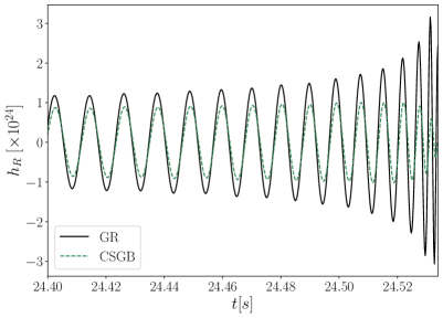
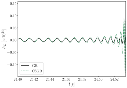
Figure 1: Example modification to a binary black hole waveform for $h_{R}$ (left) and $h_{L}$ (right). We see a constant phase shift across both polarizations due to the parity-invariant modification to the phase, and an attenuation/enhancement of the amplitude for $h_{R}$ and $h_{L}$, respectively, due to the parity-violating modification to the amplitude. To generate the waveform, we employ the GW Analysis Tools code Perkins et al. (2021). For the source parameters we take $m_{1}=20M_{\odot}$, $m_{2}=18M_{\odot}$, $\iota=2.6$ rad, $\psi=3.14$ rad, $RA=3.45$ rad, $Dec=-3968$ rad. For computational ease we rescale $f/100$ Hz, and $D_{2}/\text{Gpc}$. The modification parameters are chosen to be artificially large in order to visually see the effects; in dimensionless units $\phi_{0}^{\prime}=3$ and $\varphi_{0}^{\prime}=5$.

Furthermore, we can see how the GW velocity is modified for CS-GB gravity. From Eqs. (44) and (48), the GWs satisfy the dispersion relation

$$\omega_{R,L}^{2}=k^{2}\bigg{[}1-\frac{\alpha^{\prime}}{2}\bigg{(}\frac{1}{a}\mathcal{H}\phi^{\prime}+\varphi^{\prime 2}\bigg{)}\bigg{]}.$$ (62)

From Eq. (62), we can find the group and phase velocities of a GW, which are given by $v_{g}=d\omega/dk$ and $v_{p}=\omega/k$, respectively. We have

$$v_{g}^{R,L}=v_{p}^{R,L}=1-\frac{\alpha^{\prime}}{4}\bigg{(}\frac{1}{a}\mathcal{H}\phi^{\prime}+\varphi^{\prime 2}\bigg{)}.$$ (63)

In Appendix C, we show how Eq. (63) can be generalized for any extension to GR, using the framework that is presented in the next section.

VI Extension of Parity-Violating Parametrization and Constraints

In this section, we place our work in a broader context by making contact with the parametrization in Jenks et al. (2023) in Sec. VI.1 and then discussing observational constraints on the theory in Sec VI.2.

VI.1 Parametrization

We would like to place our work in the context of the parametrization in Jenks et al. (2023), in which it was shown that generic parity-violating corrections to the GW propagation equations can be written in a theory-agnostic way using dimensionless parameters; a particular theory will then correspond to specific values of these parameters.

In our expression Eq. (44), because we have contributions from both the CS and GB corrections, we have both parity-even and parity-odd terms. Thus, we can extend the parametrization in Jenks et al. (2023) to also account for parity-invariant terms such that the GW propagation equation can be written as

$$h_{R,L}^{\prime\prime}~{}+~{}\bigg{\{}2\mathcal{H}~{}+~{}\sum_{n=1}^{\infty}(\lambda_{R,L}k)^{n}\bigg{[}\frac{\alpha_{n}(\eta)}{(\Lambda_{PV}a)^{n}}\mathcal{H}~{}+~{}\frac{\beta_{n}(\eta)}{(\Lambda_{PV}a)^{n-1}}\bigg{]}\bigg{\}}h_{R,L}^{\prime}$$

$$+~{} k^{2}\bigg{\{}1~{}+~{}\sum_{m=0}^{\infty}(\lambda_{R,L})^{m+1}k^{m-1}\bigg{[}\frac{\gamma_{m}(\eta)}{(\Lambda_{PV}a)^{m}}\mathcal{H}~{}+~{}\frac{\delta_{m}(\eta)}{(\Lambda_{PV}a)^{m-1}}\bigg{]}\bigg{\}}h_{R,L}=0,$$ (64)

where $\{\alpha_{n},\beta_{n},\gamma_{m},\delta_{m}\}$ are the dimensionless parameters that depend on the specific theory in consideration, and $\Lambda_{PV}$ is the cutoff scale of the theory. When $\alpha=\beta=\gamma=\delta=0$, we recover the propagation equation for GWs in GR. In CS gravity, for example, the parameter $\alpha_{1}\neq 0$ with all other parameters vanishing.

Here $m$ and $n$ are integers; this extends the parametrization in Jenks et al. (2023) in which $n$ and $m$ were constrained to be odd and even integers, respectively, as to consider only parity violating effects. With this extension, one can now explicitly see the propagation effects of theories with both parity-violating and parity-invariant contributions. This extension also cleanly maps to ppE Yunes and Pretorius (2009b) and can be easily used in data analysis.

Comparing Eq. (64) with Eqs. (47) and (48), we can make the identification that $\alpha_{1}=-2\alpha^{\prime}\tilde{\varphi}^{\prime}$, $\beta_{1}=2\alpha^{\prime}\phi^{\prime}\varphi^{\prime}$, $\gamma_{1}=-\frac{1}{2}\alpha^{\prime}\tilde{\phi}^{\prime}$ and $\delta_{1}=-\frac{1}{2}\alpha^{\prime}\varphi^{\prime 2}$, with all other parameters being zero, where we have introduced a rescaling of the scalar fields by $\Lambda_{PV}$ such that $\tilde{\phi}\equiv\phi\Lambda_{PV}$ and $\tilde{\varphi}\equiv\varphi\Lambda_{PV}$.

VI.2 Constraints

While a full data analysis will be necessary to rigorously constrain $\phi^{\prime}$ and $\varphi^{\prime}$, as a first step, we can consider initial constraints based on previously existing work in the literature. Sigificant work has been done to constrain birefringent effects from a variety of GW sources, e.g. Okounkova et al. (2022); Zhao et al. (2022); Ng et al. (2023); Callister et al. (2023); Lagos et al. (2024). Here, we consider both the velocity constraints from the GW170817/GRB170817 coincident event and birefringence specific constraints in the literature from binary black hole events.

The coincident GW/gamma ray burst event from the binary neutron star merger GW170817 has provided a tight constraint on the speed of GWs, $c_{T}$, compared to the speed of light, $c$. We have Abbott et al. (2017)

$$-7\times 10^{-16}<1-c_{T}<3\times 10^{-15}.$$ (65)

From Eq. (63), we have

$$|v_{g}-1|=\frac{\alpha^{\prime}}{4}\bigg{(}\frac{1}{a}\mathcal{H}\phi^{\prime}+\varphi^{\prime 2}\bigg{)}.$$ (66)

Taking the weaker constraint of Eq. (65), and neglecting the term that is suppressed by $\mathcal{H}/\Lambda_{PV}$ in Eq. (66), we have

$$\bigg{|}\frac{1}{4}\alpha^{\prime}\varphi^{\prime 2}\bigg{|}<3\times 10^{-15}.$$ (67)

One can combine Eq. (67) with constraints on $\alpha^{\prime}$ from GB gravity (see e.g. Wang et al. (2021); Lyu et al. (2022)) to obtain a bound on $\varphi^{\prime}$, which is roughly $\tilde{\varphi}^{\prime}\lesssim 10^{-15}~{}\text{eV}^{2}$ (in natural units).

We can then use the constraint from Ng et al. (2023) via Jenks et al. (2023),

$$\bigg{|}2\alpha^{\prime}\phi_{0}^{\prime}\varphi_{0}^{\prime}\bigg{|}<0.7\times 10^{-20},$$ (68)

and combining Eq. (68) with Eq. (67) allows one to place a constraint on $\phi_{0}^{\prime}$, which is roughly $\tilde{\phi}^{\prime}_{0}\lesssim 10^{-22}~{}\text{eV}^{2}$.

VII Discussion and Conclusions

In this work, we have studied the propagation of GWs in CS-GB gravity. We have reviewed the derivation of CS-GB gravity from HST and derived how GW propagation is modified in such a theory. We have furthermore extended the parametrization first introduced in Jenks et al. (2023) for the parity-violating sector to include the parity-even sector. The framework presented in this paper thus allows one to study any correction to GR in explicitly parity-violating and parity-invariant contributions. Moreover, we have used this parametrization to map the CS-GB modifications to GW observables, which allows us to place constraints on the theory parameters.

As we have seen, CS-GB gravity (and modified gravity theories in general) will modify both the amplitude and phase of a GW. Most of this paper has focused on these modifications for the propagation of a GW, but these modifications can also arise in the generation of GWs. In compact binary coalescences, the presence of the axion and dilaton will extract energy from the binary, leading to a modification of the chirp mass (see e.g. Yunes and Pretorius (2009a); Sopuerta and Yunes (2009); Yagi et al. (2012); Alexander and Yunes (2018)). The two effects can be considered independently, with the generation effects being of $\mathcal{O}(\alpha^{\prime 2})$, making them subdominant to the propagation effects, which are of $\mathcal{O}(\alpha^{\prime})$ Callister et al. (2023).

Furthermore, CS-GB gravity can impact GWs during inflation. For example, tensor perturbations of the spacetime metric source primordial GWs, which encode important information of the early Universe and provide an important test of GR. During inflation, the Pontryagin term associated with CS gravity can lead to the resonant amplification of GWs on small scales Peng et al. (2022), and one can study the energy spectrum associated with these GWs Odintsov et al. (2022). It would be interesting to determine how these scenarios would be modified in CS-GB gravity. We leave this study for future work.

The gravitational field in the exterior of supermassive, spinning black holes (BHs) is crucial in the emission of GWs. In GR, such a field is described by the Kerr metric Kerr (1963), which is a stationary and axisymmetric solution, parametrized in terms of the mass of the BH and its angular momentum. However, in modified theories of gravity, the Kerr metric does not need to be a solution to the field equations. For example, in the case of GB gravity, slowly rotating BH solutions have been found that differ from Kerr Pani and Cardoso (2009). A measured deviation from the Kerr metric, whether from electromagnetic or GW observations Psaltis et al. (2008); Psaltis (2008); Glampedakis and Babak (2006); Collins and Hughes (2004), can therefore provide insight into extensions of GR, or lack thereof.

One can ask what metric represents a spinning BH in CS-GB gravity. For CS, the metric and scalar field perturbations describing the leading order corrections to the Kerr metric are known Yunes and Pretorius (2009a); Delsate et al. (2018). The leading order corrections for GB have been analyzed as well Kleihaus et al. (2011); Maselli et al. (2015); Kleihaus et al. (2016). We leave an in-depth analysis of the BH solution in CS-GB gravity for future work.

Appendix A Stringy Derivation

In this appendix, we provide more details on the derivation of the 4D effective action Eq. (29) in Sec. III, following Cano and Ruipérez (2022).

With the CS term in the 10D heterotic superstring effective action (Eq. (20)), $\hat{H}$ satisfies the modified Bianchi identity,

$$d\hat{H}=\frac{\alpha^{\prime}}{4}\hat{R}_{(-)~{}~{}b}^{~{}~{}~{}~{}a}\wedge\hat{R}_{(-)~{}a}^{~{}~{}b}.$$ (69)

Upon compactifying Eq. (20) on a six-torus in Eq. (23), Eq. (69) can be written as

$$\frac{1}{3!}\epsilon^{\mu\nu\rho\sigma}\bar{\nabla}_{\mu}H_{\nu\rho\sigma}+\frac{\alpha^{\prime}}{8}\bar{R}_{(-)\nu\rho\sigma}\tilde{\bar{R}}_{(-)}^{\mu\nu\rho\sigma}=0,$$ (70)

where

$$\tilde{\bar{R}}_{(-)}^{\mu\nu\rho\sigma}=\frac{1}{2}\epsilon^{\mu\nu\alpha\beta}\bar{R}_{(-)\alpha\beta}^{~{}~{}~{}~{}~{}~{}\rho\sigma}.$$ (71)

After integrating by parts, we get Eq. (24):

$$\bar{S} =\frac{1}{16\pi G_{N}^{(4)}}\int d^{4}x\sqrt{|\bar{g}|}\bigg{\{}e^{-2(\hat{\phi}-\hat{\phi}_{\infty})}\bigg{[}\bar{R}-4(\partial\hat{\phi})^{2}$$

$$+\frac{1}{12}H^{2}\bigg{]}-\frac{1}{3!}H_{\mu\nu\rho}\epsilon^{\mu\nu\rho\sigma}\partial_{\sigma}\varphi+\frac{\alpha^{\prime}}{8}\mathcal{L}_{R^{2}}+\mathcal{O}(\alpha^{\prime 3})\bigg{\}},$$ (72)

where

$$\mathcal{L}_{R^{2}}=e^{-2(\hat{\phi}-\hat{\phi}_{\infty})}\bar{R}_{(-)\mu\nu\rho\sigma}\bar{R}_{(-)}^{\mu\nu\rho\sigma}-\varphi\bar{R}_{(-)\mu\nu\rho\sigma}\tilde{\bar{R}}_{(-)}^{{\mu\nu\rho\sigma}}.$$ (73)

Now, from the variation of $H$, we have that

$$e^{-2(\hat{\phi}-\hat{\phi}_{\infty})}\frac{1}{6}H_{\mu\nu\rho}-\frac{1}{6}\epsilon_{\mu\nu\rho\sigma}\bar{\nabla}^{\sigma}\varphi+\frac{\alpha^{\prime}}{8}\frac{\delta\mathcal{L}_{R^{2}}}{\delta H^{\mu\nu\rho}}=0,$$ (74)

and as explained in Section III, to solve it we expand $H$ in $\alpha^{\prime}$:

$$H=H^{(0)}+\alpha^{\prime}H^{(1)}+\alpha^{\prime 2}H^{(2)}+...,$$ (75)

which after plugging the expansion Eq. (75) into Eq. (72), we arrive at Eq. (26),

$$\bar{S} =\frac{1}{16\pi G_{N}^{(4)}}\int d^{4}x\bigg{\{}e^{-2(\hat{\phi}-\hat{\phi}_{\infty})}\bigg{[}\bar{R}-4(\partial\hat{\phi})^{2}\bigg{]}$$

$$+\frac{1}{2}e^{2(\hat{\phi}-\hat{\phi}_{\infty})}(\partial\varphi)^{2}+\frac{\alpha^{\prime}}{8}\mathcal{L}_{R^{2}}\biggr{\rvert}_{H^{(0)}}+\mathcal{O}(\alpha^{\prime 2})\bigg{\}}.$$ (76)

To evaluate the four-derivative term $\mathcal{L}_{R^{2}}$, we have to substitute in the expression for $H^{(0)}$, which is

$$H_{\mu\nu\rho}^{(0)}=e^{2(\hat{\phi}-\hat{\phi}_{\infty})}\epsilon_{\mu\nu\rho\sigma}\nabla^{\sigma}\varphi,$$ (77)

and use the fact that the curvature $\hat{R}_{(-)}$ can be written in terms of $\hat{H}$ as well as the Riemannian curvature $\hat{R}$:

$$\hat{R}_{(-)\mu\nu~{}\sigma}^{~{}~{}~{}~{}~{}~{}\rho} =\hat{R}_{\mu\nu~{}\sigma}^{~{}~{}~{}\rho}-\hat{\nabla}_{[\mu}\hat{H}_{\nu]~{}~{}\sigma}^{~{}~{}\rho}-\frac{1}{2}\hat{H}_{[\mu|~{}\alpha}^{~{}\rho}\hat{H}_{|\nu]~{}\sigma}^{~{}~{}\alpha}.$$ (78)

Evaluation of the four-derivative term yields Eq. (27),

$$\mathcal{L}_{R^{2}}\biggr{\rvert}_{H^{(0)}} =e^{-2(\hat{\phi}-\hat{\phi}_{\infty})}\bigg{[}\bar{R}_{\mu\nu\rho\sigma}\bar{R}^{\mu\nu\rho\sigma}+6\bar{G}_{\mu\nu}A^{\mu}A^{\nu}+\frac{7}{4}A^{4}$$

$$-2\bar{\nabla}_{\mu}A_{\nu}\bar{\nabla}^{\mu}A^{\nu}-(\bar{\nabla}_{\mu}A^{\mu})^{2}\bigg{]}-\varphi\bar{R}_{\mu\nu\rho\sigma}\tilde{\bar{R}}^{\mu\nu\rho\sigma}$$

$$+\text{total derivatives}.$$ (79)

Upon transforming our theory from the Jordan frame to the Einstein frame via the conformal rescaling Eq. (28), the effect on the two-derivative terms in the Lagrangian is rather straightforward to compute:

$$\sqrt{|\bar{g}|}\mathcal{L}_{2}=\sqrt{|g|}\bigg{[}R+2(\partial\hat{\phi})^{2}+\frac{1}{2}e^{4(\hat{\phi}-\hat{\phi}_{\infty})}(\partial\varphi)^{2}\bigg{]}.$$ (80)

On the other hand, the effect of the conformal rescaling on the four-derivative term $\mathcal{L}_{R^{2}}$ requires a lengthier calculation; we need to take into account the transformation of the Riemann tensor and the covariant derivative, and integrate by parts multiple times. The end result is

$$\sqrt{|\bar{g}|} \mathcal{L}_{R^{2}}\biggr{\rvert}_{H^{(0)}}=\sqrt{|g|}\bigg{\{}e^{-2(\hat{\phi}-\hat{\phi}_{\infty}})\bigg{[}R_{\mu\nu\rho\sigma}R^{\mu\nu\rho\sigma}$$

$$+~{} 4R^{\mu\nu}(4\partial_{\mu}\hat{\phi}\partial_{\nu}\hat{\phi}+A_{\mu}A_{\nu})+R[4\nabla^{2}\hat{\phi}-4(\partial\hat{\phi})^{2}-3A^{2}]$$

$$+~{} 12(\partial\hat{\phi})^{4}+12(\nabla^{2}\hat{\phi})^{2}+\frac{7}{4}A^{4}-12(\partial_{\mu}\hat{\phi}A^{\mu})^{2}$$

$$-~{} 2A^{2}(\partial\hat{\phi})^{2}-8A^{2}\nabla^{2}\hat{\phi}-16\partial_{\mu}\hat{\phi}A^{\mu}\nabla_{\alpha}A^{\alpha}-3(\nabla_{\alpha}A^{\alpha})^{2}\bigg{]}$$

$$-~{} \varphi R_{\mu\nu\rho\sigma}\tilde{R}^{\mu\nu\rho\sigma}\bigg{\}}+\text{total derivatives},$$ (81)

which we can rewrite as

$$\sqrt{\overline{\bar{g}}}\mathcal{L}_{R^{2}}\biggr{\rvert}_{H^{(0)}}=\sqrt{\bar{g}}\bigg{[}e^{-2(\hat{\phi}-\hat{\phi}_{\infty})}\mathcal{X}_{4}-\varphi R_{\mu\nu\rho\sigma}\tilde{R}^{\mu\nu\rho\sigma}+\mathcal{L}^{\prime}\bigg{]},$$ (82)

where $\mathcal{X}_{4}=R^{2}-4R_{\mu\nu}R^{\mu\nu}+R_{\mu\nu\rho\sigma}R^{\mu\nu\rho\sigma}$ is the 4D GB density, and we have collected the remaining terms in $\mathcal{L}^{\prime}$.

Now, let us consider the zeroth order equations of motion

$$\mathcal{E}_{\mu\nu} =R_{\mu\nu}+2\partial_{\mu}\hat{\phi}\partial_{\nu}\hat{\phi}+\frac{1}{2}A_{\mu}A_{\nu},$$ (83)

$$\mathcal{E}_{\hat{\phi}} =\nabla^{2}\hat{\phi}-\frac{1}{2}A^{2},$$ (84)

$$\mathcal{E}_{\varphi} =\nabla_{\mu}A^{\mu}+2\partial_{\mu}\hat{\phi}A^{\mu}.$$ (85)

After some algebra, $\mathcal{L}^{\prime}$ can be written in terms of Eqs. (83)-(85) as follows:

$$\mathcal{L}^{\prime} =e^{-2(\hat{\phi}-\hat{\phi}_{\infty})}\bigg{\{}4\mathcal{E}_{\mu\nu}\mathcal{E}^{\mu\nu}-\mathcal{E}^{2}+12\mathcal{E}_{\hat{\phi}}^{2}+4\mathcal{E}\mathcal{E}_{\hat{\phi}}-3\mathcal{E}_{\varphi}^{2}$$

$$+2\mathcal{E}_{\hat{\phi}}[A^{2}-4(\partial\hat{\phi})^{2}]-4\mathcal{E}_{\varphi}\partial_{\mu}\hat{\phi}A^{\mu}\bigg{\}}.$$ (86)

We see that all the terms in $\mathcal{L}^{\prime}$ are proportional to the zeroth-order equations of motion, which means if we redefine the fields

$$g_{\mu\nu} \rightarrow g_{\mu\nu}+\alpha^{\prime}\Delta_{\mu\nu},$$ (87)

$$\hat{\phi} \rightarrow\hat{\phi}+\alpha^{\prime}\Delta\hat{\phi},$$ (88)

$$\varphi \rightarrow\varphi+\alpha^{\prime}\Delta\varphi,$$ (89)

then we introduce terms linear in $\alpha^{\prime}$ that are proportional to the zeroth order equations of motion, which we can therefore use to cancel all the terms in $\mathcal{L}^{\prime}$ Cano and Ruipérez (2022).

Thus, introducing the 4D dilaton $\phi=2(\hat{\phi}-\hat{\phi}_{\infty})$, we end up with Eq. (29), a very simple form of our action in four dimensions:

$$S =\frac{1}{16\pi}\int d^{4}x\sqrt{|g|}\bigg{[}R+\frac{1}{2}(\partial\phi)^{2}+\frac{1}{2}e^{2\phi}(\partial\varphi)^{2}$$

$$+\frac{\alpha^{\prime}}{8}\bigg{(}e^{-\phi}\mathcal{X}_{4}-\varphi R_{\mu\nu\rho\sigma}\tilde{R}^{\mu\nu\rho\sigma}\bigg{)}+\mathcal{O}(\alpha^{\prime 2})\bigg{]}.$$ (90)

Appendix B Taylor Expansion for GW Propagation Coefficients

Here we show the steps in expanding the $\bar{B}$ and $\bar{C}$ coefficients in Eq. (44) to linear order in $\alpha^{\prime}$.

For $\bar{B}$, we have

$$\bar{B} \approx\bigg{(}1+\frac{\alpha^{\prime}}{4a^{2}}\phi^{\prime\prime}+\frac{\alpha^{\prime}a^{2}}{2}\lambda_{R,L}k\varphi^{\prime}\bigg{)}\bigg{[}2\mathcal{H}+\frac{\alpha^{\prime}}{2a^{2}}\mathcal{H}\phi^{\prime\prime}$$

$$-\lambda_{R,L}\alpha^{\prime}k\bigg{(}a^{2}\mathcal{H}\varphi^{\prime}+\frac{\varphi^{\prime\prime}}{a^{2}}\bigg{)}\bigg{]}$$ (91)

$$\approx 2\mathcal{H}+\frac{\alpha^{\prime}}{a^{2}}\mathcal{H}\phi^{\prime\prime}-\frac{\alpha^{\prime}}{a^{2}}k\lambda_{R,L}\varphi^{\prime\prime},$$ (92)

where we have assumed that $k\gg\mathcal{H}$. We can then use Eqs. (45) and (46) to obtain

$$\bar{B} =2\mathcal{H}-\lambda_{R,L}k\frac{2\alpha^{\prime}}{a^{2}}\bigg{(}\mathcal{H}\varphi^{\prime}-\phi^{\prime}\varphi^{\prime}\bigg{)}.$$ (93)

Now, we need to correct for the factors of $a$, since $(1/a)(da/d\eta)=da/dt$. Thus, the conformal time derivatives in Eq. (93) pick up an extra factor of $a$. So, we have

$$\bar{B} =2\mathcal{H}-2\lambda_{R,L}\alpha^{\prime}k\bigg{(}\frac{\mathcal{H}}{a}\varphi^{\prime}-\phi^{\prime}\varphi^{\prime}\bigg{)},$$ (94)

which is Eq. (47).

For $\bar{C}$, we have

$$\bar{C} \approx\bigg{(}1+\frac{\alpha^{\prime}}{4a^{2}}\phi^{\prime\prime}+\lambda_{R,L}\frac{\alpha^{\prime}a^{2}}{2}k\varphi^{\prime}\bigg{)}\bigg{\{}k^{2}-2\mathcal{H}^{2}+6\mathcal{H}^{\prime}$$

$$+\frac{\alpha^{\prime}}{2a^{2}}\phi^{\prime\prime}\bigg{(}4\mathcal{H}^{2}-12\mathcal{H}^{\prime}-k^{2}\bigg{)}$$

$$-\lambda_{R,L}\frac{\alpha^{\prime}}{2}k\bigg{[}a^{2}\varphi^{\prime}(4\mathcal{H}^{2}+k^{2})+\frac{2\mathcal{H}\varphi^{\prime\prime}}{a^{4}}\bigg{]}\bigg{\}}$$ (95)

$$\approx k^{2}-\frac{\alpha^{\prime}k^{2}}{4a^{2}}\phi^{\prime\prime},$$ (96)

where in going from Eq. (95) to (96) we have again assumed that $k\gg\mathcal{H}$. Furthermore, we can assume that $\phi$ and $\varphi$ are small to retain terms that are at most second-order in the scalar fields in Eq. (96).

Plugging Eq. (45) into Eq. (96) yields

$$\bar{C}=k^{2}\bigg{[}1-\frac{\alpha^{\prime}}{2a^{2}}\bigg{(}\mathcal{H}\phi^{\prime}+\varphi^{\prime 2}\bigg{)}\bigg{]},$$ (97)

and again noting that $(1/a)(da/d\eta)=da/dt$ to correct the factors of $a$ in the conformal time derivatives, we end up with

$$\bar{C} =k^{2}\bigg{[}1-\frac{\alpha^{\prime}}{2}\bigg{(}\frac{\mathcal{H}}{a}\phi^{\prime}+\varphi^{\prime 2}\bigg{)}\bigg{]},$$ (98)

which is Eq. (48).

Appendix C Generalization of Modified Dispersion Relation

The discussion in Sec. V from Eq. (50) onwards can be generalized for any modification to GR by extending the discussion in Jenks et al. (2023) to include the parity-even sector. From Eq. (19) of Jenks et al. (2023) and Eq. (64), it is straightforward to see that the effective modified dispersion relation Eq. (50) can be parametrized as

$$\theta^{\prime\prime} +\theta^{\prime 2}+i\theta^{\prime}\bigg{\{}2\mathcal{H}+(\lambda_{R,L}k)^{n}\bigg{[}\frac{\alpha_{n}}{(\Lambda_{PV}a)^{n}}\mathcal{H}+\frac{\beta_{n}}{(\Lambda_{PV}a)^{n-1}}\bigg{]}\bigg{\}}$$

$$-k^{2}\bigg{\{}1+(\lambda_{R,L})^{m+1}k^{m-1}\bigg{[}\frac{\gamma_{m}}{(\Lambda_{PV}a)^{m}}\mathcal{H}+\frac{\delta_{m}}{(\Lambda_{PV}a)^{m-1}}\bigg{]}\bigg{\}}$$

$$=0,$$ (99)

where we are keeping the sums over $n$ and $m$ implicit.

From Eq. (20) of Jenks et al. (2023), we can see that the generalization of Eq. (52) is

$$\delta\theta=-i(\lambda_{R,L})^{n}\delta\theta_{A}+(\lambda_{R,L})^{m+1}\delta\theta_{V},$$ (100)

where the amplitude and velocity birefringence contributions are

$$\delta\theta_{A}^{\prime} =\frac{k^{n}}{2}\bigg{[}\frac{\alpha_{n}}{(\Lambda_{PV}a)^{n}}\mathcal{H}+\frac{\beta_{n}}{(\Lambda_{PV}a)^{n-1}}\bigg{]},$$ (101)

$$\delta\theta_{V}^{\prime} =\frac{k^{m}}{2}\bigg{[}\frac{\gamma_{m}}{(\Lambda_{PV}a)^{m}}\mathcal{H}+\frac{\delta_{m}}{(\Lambda_{PV}a)^{m-1}}\bigg{]}.$$ (102)

Eqs. (101) and (102) can be rewritten as

$$\delta\theta_{A} =\frac{[k(1+z)]^{n}}{2}\bigg{(}\frac{\alpha_{n_{0}}}{\Lambda_{PV}^{n}}z_{n}+\frac{\beta_{n_{0}}}{\Lambda_{PV}^{n-1}}D_{n+1}\bigg{)},$$ (103)

$$\delta\theta_{V} =\frac{[k(1+z)^{m}]}{2}\bigg{(}\frac{\gamma_{m_{0}}}{\Lambda_{PV}^{m}}z_{m}+\frac{\delta_{m_{0}}}{\Lambda_{PV}^{m-1}}D_{m+1}\bigg{)},$$ (104)

such that the right and left-handed polarization modes are modified in the following way

$$h_{R,L}=\bar{h}_{R,L}$$

$$\times\text{exp}\bigg{\{}-(\lambda_{R,L})^{n}\frac{[k(1+z)]^{n}}{2}\bigg{(}\frac{\alpha_{n_{0}}}{\Lambda_{PV}^{n}}z_{n}+\frac{\beta_{n_{0}}}{\Lambda_{PV}^{n-1}}D_{n+1}\bigg{)}\bigg{\}}$$

$$\times\text{exp}\bigg{\{}i(\lambda_{R,L})^{m+1}\frac{[k(1+z)]^{m}}{2}\bigg{(}\frac{\gamma_{m_{0}}}{\Lambda_{PV}^{m}}z_{m}+\frac{\delta_{m_{0}}}{\Lambda_{PV}^{m-1}}D_{m+1}\bigg{)}\bigg{\}},$$ (105)

where $\bar{h}_{R,L}$ is the usual GR expression for the right and left-handed modes.

Via the generalized modified dispersion relation

$$\omega_{R,L}^{2}=k^{2}\bigg{\{}1+(\lambda_{R,L})^{m+1}k^{m-1}\bigg{[}\frac{\gamma_{m}}{(\Lambda_{PV}a)^{m}}\mathcal{H}+\frac{\delta_{m}}{(\Lambda_{PV}a)^{m-1}}\bigg{]}\bigg{\}},$$ (106)

the modified group and phase velocities are then

$$v_{g}^{R,L} =1+\frac{(\lambda_{R,L})^{m+1}}{2}mk^{m-1}\bigg{[}\frac{\gamma_{m}}{(a\Lambda_{PV})^{m}}\mathcal{H}+\frac{\delta_{m}}{(a\Lambda_{PV})^{m-1}}\bigg{]},$$ (107)

$$v_{p}^{R,L} =1+\frac{(\lambda_{R,L})^{m+1}}{2}k^{m-1}\bigg{[}\frac{\gamma_{m}}{(a\Lambda_{PV})^{m}}\mathcal{H}+\frac{\delta_{m}}{(a\Lambda_{PV})^{m-1}}\bigg{]}.$$ (108)

References

- Abbott et al. (2019a) B. P. Abbott, R. Abbott, T. D. Abbott, F. Acernese, K. Ackley, C. Adams, T. Adams, P. Addesso, R. X. Adhikari, V. B. Adya, et al. (LIGO Scientific Collaboration and Virgo Collaboration), Phys. Rev. Lett. 123, 011102 (2019a), URL https://link.aps.org/doi/10.1103/PhysRevLett.123.011102.
- Abbott et al. (2019b) B. P. Abbott, R. Abbott, T. D. Abbott, S. Abraham, F. Acernese, K. Ackley, C. Adams, R. X. Adhikari, V. B. Adya, C. Affeldt, et al. (The LIGO Scientific Collaboration and the Virgo Collaboration), Phys. Rev. D 100, 104036 (2019b), URL https://link.aps.org/doi/10.1103/PhysRevD.100.104036.
- Abbott et al. (2021a) R. Abbott, T. D. Abbott, S. Abraham, F. Acernese, K. Ackley, A. Adams, C. Adams, R. X. Adhikari, V. B. Adya, C. Affeldt, et al. (LIGO Scientific Collaboration and Virgo Collaboration), Phys. Rev. D 103, 122002 (2021a), URL https://link.aps.org/doi/10.1103/PhysRevD.103.122002.
- Collaboration et al. (2021) T. L. S. Collaboration, the Virgo Collaboration, the KAGRA Collaboration, R. Abbott, H. Abe, F. Acernese, K. Ackley, N. Adhikari, R. X. Adhikari, V. K. Adkins, et al., Tests of general relativity with gwtc-3 (2021), eprint 2112.06861.
- Will (2014) C. M. Will, Living Reviews in Relativity 17 (2014), ISSN 1433-8351, URL http://dx.doi.org/10.12942/lrr-2014-4.
- Alexander et al. (2021) S. Alexander, G. Gabadadze, L. Jenks, and N. Yunes, Physical Review D 104 (2021), ISSN 2470-0029, URL http://dx.doi.org/10.1103/PhysRevD.104.064033.
- Shapiro (1990) I. I. Shapiro (1990), URL https://api.semanticscholar.org/CorpusID:117428821.
- S. and M.-T. (2009) R. S. and J. M.-T., Proceedings of the International School of Physics 168, 203–217 (2009), ISSN 0074-784X, URL https://doi.org/10.3254/978-1-58603-990-5-203.
- Abbott et al. (2019c) B. P. Abbott, R. Abbott, T. D. Abbott, S. Abraham, F. Acernese, K. Ackley, C. Adams, R. X. Adhikari, V. B. Adya, C. Affeldt, et al. (LIGO Scientific Collaboration and Virgo Collaboration), Phys. Rev. X 9, 031040 (2019c), URL https://link.aps.org/doi/10.1103/PhysRevX.9.031040.
- Abbott et al. (2021b) R. Abbott, T. D. Abbott, S. Abraham, F. Acernese, K. Ackley, A. Adams, C. Adams, R. X. Adhikari, V. B. Adya, C. Affeldt, et al. (LIGO Scientific Collaboration and Virgo Collaboration), Phys. Rev. X 11, 021053 (2021b), URL https://link.aps.org/doi/10.1103/PhysRevX.11.021053.
- Abbott et al. (2023) R. Abbott, T. D. Abbott, F. Acernese, K. Ackley, C. Adams, N. Adhikari, R. X. Adhikari, V. B. Adya, C. Affeldt, D. Agarwal, et al. (LIGO Scientific Collaboration, Virgo Collaboration, and KAGRA Collaboration), Phys. Rev. X 13, 041039 (2023), URL https://link.aps.org/doi/10.1103/PhysRevX.13.041039.
- Abbott et al. (2017) B. P. Abbott, R. Abbott, T. D. Abbott, F. Acernese, K. Ackley, C. Adams, T. Adams, P. Addesso, R. X. Adhikari, V. B. Adya, et al., The Astrophysical Journal Letters 848, L13 (2017), ISSN 2041-8213, URL http://dx.doi.org/10.3847/2041-8213/aa920c.
- Capozziello and De Laurentis (2011) S. Capozziello and M. De Laurentis, Physics Reports 509, 167–321 (2011), ISSN 0370-1573, URL http://dx.doi.org/10.1016/j.physrep.2011.09.003.
- Faraoni and Capozziello (2011) V. Faraoni and S. Capozziello, Beyond Einstein Gravity: A Survey of Gravitational Theories for Cosmology and Astrophysics (Springer, Dordrecht, 2011), ISBN 978-94-007-0164-9, 978-94-007-0165-6.
- Nojiri and Odintsov (2007) S. Nojiri and S. D. Odintsov, International Journal of Geometric Methods in Modern Physics 04, 115–145 (2007), ISSN 1793-6977, URL http://dx.doi.org/10.1142/S0219887807001928.
- Nojiri et al. (2017) S. Nojiri, S. Odintsov, and V. Oikonomou, Physics Reports 692, 1–104 (2017), ISSN 0370-1573, URL http://dx.doi.org/10.1016/j.physrep.2017.06.001.
- Boulware and Deser (1986) D. G. Boulware and S. Deser, Phys. Lett. B 175, 409 (1986).
- Kanti et al. (1996) P. Kanti, N. E. Mavromatos, J. Rizos, K. Tamvakis, and E. Winstanley, Phys. Rev. D 54, 5049 (1996), URL https://link.aps.org/doi/10.1103/PhysRevD.54.5049.
- Torii et al. (1997) T. Torii, H. Yajima, and K.-i. Maeda, Phys. Rev. D 55, 739 (1997), URL https://link.aps.org/doi/10.1103/PhysRevD.55.739.
- Alexeyev and Pomazanov (1997) S. O. Alexeyev and M. V. Pomazanov, Phys. Rev. D 55, 2110 (1997), URL https://link.aps.org/doi/10.1103/PhysRevD.55.2110.
- Starobinsky (1980) A. A. Starobinsky, Phys. Lett. B 91, 99 (1980).
- Sotiriou and Faraoni (2010) T. P. Sotiriou and V. Faraoni, Reviews of Modern Physics 82, 451–497 (2010), ISSN 1539-0756, URL http://dx.doi.org/10.1103/RevModPhys.82.451.
- Lue et al. (1999) A. Lue, L. Wang, and M. Kamionkowski, Physical Review Letters 83, 1506–1509 (1999), ISSN 1079-7114, URL http://dx.doi.org/10.1103/PhysRevLett.83.1506.
- Jackiw and Pi (2003) R. Jackiw and S.-Y. Pi, Phys. Rev. D 68, 104012 (2003), URL https://link.aps.org/doi/10.1103/PhysRevD.68.104012.
- Alexander and Yunes (2009) S. Alexander and N. Yunes, Physics Reports 480, 1–55 (2009), ISSN 0370-1573, URL http://dx.doi.org/10.1016/j.physrep.2009.07.002.
- Yunes and Pretorius (2009a) N. Yunes and F. Pretorius, Phys. Rev. D 79, 084043 (2009a), URL https://link.aps.org/doi/10.1103/PhysRevD.79.084043.
- Crisostomi et al. (2018) M. Crisostomi, K. Noui, C. Charmousis, and D. Langlois, Phys. Rev. D 97, 044034 (2018), eprint 1710.04531.
- Conroy and Koivisto (2019) A. Conroy and T. Koivisto, Journal of Cosmology and Astroparticle Physics 2019, 016–016 (2019), ISSN 1475-7516, URL http://dx.doi.org/10.1088/1475-7516/2019/12/016.
- Hořava (2009) P. Hořava, Phys. Rev. D 79, 084008 (2009), URL https://link.aps.org/doi/10.1103/PhysRevD.79.084008.
- Zhu et al. (2013) T. Zhu, W. Zhao, Y. Huang, A. Wang, and Q. Wu, Phys. Rev. D 88, 063508 (2013), URL https://link.aps.org/doi/10.1103/PhysRevD.88.063508.
- Nishizawa and Kobayashi (2018) A. Nishizawa and T. Kobayashi, Phys. Rev. D 98, 124018 (2018), eprint 1809.00815.
- Manton and Alexander (2024) T. Manton and S. Alexander, The kalb-ramond field and gravitational parity violation (2024), eprint 2401.14452.
- Alvarez-Gaume and Witten (1984) L. Alvarez-Gaume and E. Witten, Nucl. Phys. B 234, 269 (1984).
- Weinberg (2013) S. Weinberg, The quantum theory of fields. Vol. 2: Modern applications (Cambridge University Press, 2013), ISBN 978-1-139-63247-8, 978-0-521-67054-8, 978-0-521-55002-4.
- Alexander et al. (2006) S. H. S. Alexander, M. E. Peskin, and M. M. Sheikh-Jabbari, Phys. Rev. Lett. 96, 081301 (2006), URL https://link.aps.org/doi/10.1103/PhysRevLett.96.081301.
- Alexander and Gates (2006) S. H. S. Alexander and S. J. Gates, Journal of Cosmology and Astroparticle Physics 2006, 018–018 (2006), ISSN 1475-7516, URL http://dx.doi.org/10.1088/1475-7516/2006/06/018.
- Green and Schwarz (1984) M. B. Green and J. H. Schwarz, Phys. Lett. B 149, 117 (1984).
- Green and Schwarz (1985) M. B. Green and J. H. Schwarz, Phys. Lett. B 151, 21 (1985).
- Green et al. (1988a) M. B. Green, J. H. Schwarz, and E. Witten, SUPERSTRING THEORY. VOL. 2: LOOP AMPLITUDES, ANOMALIES AND PHENOMENOLOGY (1988a), ISBN 978-0-521-35753-1.
- Ashtekar and Lewandowski (2004) A. Ashtekar and J. Lewandowski, Classical and Quantum Gravity 21, R53–R152 (2004), ISSN 1361-6382, URL http://dx.doi.org/10.1088/0264-9381/21/15/R01.
- Thiemann (2001) T. Thiemann, Introduction to modern canonical quantum general relativity (2001), eprint gr-qc/0110034.
- Rovelli (2004) C. Rovelli, Quantum gravity, Cambridge Monographs on Mathematical Physics (Univ. Pr., Cambridge, UK, 2004).
- Alexander and Creque-Sarbinowski (2023) S. Alexander and C. Creque-Sarbinowski, Phys. Rev. D 108, 104046 (2023), URL https://link.aps.org/doi/10.1103/PhysRevD.108.104046.
- Wu et al. (2009) E. Y. S. Wu, P. Ade, J. Bock, M. Bowden, M. L. Brown, G. Cahill, P. G. Castro, S. Church, T. Culverhouse, R. B. Friedman, et al. (QUaD Collaboration), Phys. Rev. Lett. 102, 161302 (2009), URL https://link.aps.org/doi/10.1103/PhysRevLett.102.161302.
- Sorbo (2011) L. Sorbo, Journal of Cosmology and Astroparticle Physics 2011, 003–003 (2011), ISSN 1475-7516, URL http://dx.doi.org/10.1088/1475-7516/2011/06/003.
- Shiraishi et al. (2013) M. Shiraishi, A. Ricciardone, and S. Saga, Journal of Cosmology and Astroparticle Physics 2013, 051–051 (2013), ISSN 1475-7516, URL http://dx.doi.org/10.1088/1475-7516/2013/11/051.
- Shiraishi (2016) M. Shiraishi, Physical Review D 94 (2016), ISSN 2470-0029, URL http://dx.doi.org/10.1103/PhysRevD.94.083503.
- Philcox (2023) O. H. E. Philcox, Phys. Rev. Lett. 131, 181001 (2023), URL https://link.aps.org/doi/10.1103/PhysRevLett.131.181001.
- Contaldi et al. (2008) C. R. Contaldi, J. a. Magueijo, and L. Smolin, Phys. Rev. Lett. 101, 141101 (2008), URL https://link.aps.org/doi/10.1103/PhysRevLett.101.141101.
- Alexander and Yunes (2018) S. H. Alexander and N. Yunes, Phys. Rev. D 97, 064033 (2018), URL https://link.aps.org/doi/10.1103/PhysRevD.97.064033.
- Loutrel and Yunes (2022) N. Loutrel and N. Yunes, Phys. Rev. D 106, 064009 (2022), URL https://link.aps.org/doi/10.1103/PhysRevD.106.064009.
- Lanczos (1932) C. Lanczos, Zeitschrift fur Physik 73, 147 (1932).
- Lanczos (1938) C. Lanczos, Annals Math. 39, 842 (1938).
- Lovelock (1970) D. Lovelock, Aequat. Math. 4, 127 (1970).
- Lovelock (1971) D. Lovelock, J. Math. Phys. 12, 498 (1971).
- Zwiebach (1985) B. Zwiebach, Phys. Lett. B 156, 315 (1985).
- Gross and Sloan (1987) D. J. Gross and J. H. Sloan, Nucl. Phys. B 291, 41 (1987).
- Nepomechie (1985) R. I. Nepomechie, Phys. Rev. D 32, 3201 (1985).
- Callan et al. (1986) C. G. Callan, Jr., I. R. Klebanov, and M. J. Perry, Nucl. Phys. B 278, 78 (1986).
- Candelas et al. (1985) P. Candelas, G. T. Horowitz, A. Strominger, and E. Witten, Nucl. Phys. B 258, 46 (1985).
- Moura and Schiappa (2006) F. Moura and R. Schiappa, Classical and Quantum Gravity 24, 361–386 (2006), ISSN 1361-6382, URL http://dx.doi.org/10.1088/0264-9381/24/2/006.
- Guo et al. (2008) Z.-K. Guo, N. Ohta, and T. Torii, Progress of Theoretical Physics 120, 581–607 (2008), ISSN 1347-4081, URL http://dx.doi.org/10.1143/PTP.120.581.
- Maeda et al. (2009) K.-i. Maeda, N. Ohta, and Y. Sasagawa, Physical Review D 80 (2009), ISSN 1550-2368, URL http://dx.doi.org/10.1103/PhysRevD.80.104032.
- Pani and Cardoso (2009) P. Pani and V. Cardoso, Physical Review D 79 (2009), ISSN 1550-2368, URL http://dx.doi.org/10.1103/PhysRevD.79.084031.
- Kleihaus et al. (2011) B. Kleihaus, J. Kunz, and E. Radu, Physical Review Letters 106 (2011), ISSN 1079-7114, URL http://dx.doi.org/10.1103/PhysRevLett.106.151104.
- Ayzenberg and Yunes (2014) D. Ayzenberg and N. Yunes, Phys. Rev. D 90, 044066 (2014), [Erratum: Phys.Rev.D 91, 069905 (2015)], eprint 1405.2133.
- Maselli et al. (2015) A. Maselli, P. Pani, L. Gualtieri, and V. Ferrari, Phys. Rev. D 92, 083014 (2015), URL https://link.aps.org/doi/10.1103/PhysRevD.92.083014.
- Kleihaus et al. (2016) B. Kleihaus, J. Kunz, S. Mojica, and E. Radu, Phys. Rev. D 93, 044047 (2016), URL https://link.aps.org/doi/10.1103/PhysRevD.93.044047.
- Kokkotas et al. (2017) K. D. Kokkotas, R. A. Konoplya, and A. Zhidenko, Phys. Rev. D 96, 064004 (2017), URL https://link.aps.org/doi/10.1103/PhysRevD.96.064004.
- Kanti et al. (2015) P. Kanti, R. Gannouji, and N. Dadhich, Physical Review D 92 (2015), ISSN 1550-2368, URL http://dx.doi.org/10.1103/PhysRevD.92.041302.
- Chakraborty et al. (2018) S. Chakraborty, T. Paul, and S. SenGupta, Phys. Rev. D 98, 083539 (2018), URL https://link.aps.org/doi/10.1103/PhysRevD.98.083539.
- Odintsov and Oikonomou (2018) S. D. Odintsov and V. K. Oikonomou, Phys. Rev. D 98, 044039 (2018), URL https://link.aps.org/doi/10.1103/PhysRevD.98.044039.
- Yi and Gong (2019) Z. Yi and Y. Gong, Universe 5, 200 (2019), eprint 1811.01625.
- Odintsov and Oikonomou (2019) S. Odintsov and V. Oikonomou, Physics Letters B 797, 134874 (2019), ISSN 0370-2693, URL http://dx.doi.org/10.1016/j.physletb.2019.134874.
- Rashidi and Nozari (2020) N. Rashidi and K. Nozari, The Astrophysical Journal 890, 58 (2020), ISSN 1538-4357, URL http://dx.doi.org/10.3847/1538-4357/ab6a10.
- Green et al. (1988b) M. B. Green, J. H. Schwarz, and E. Witten, SUPERSTRING THEORY. VOL. 1: INTRODUCTION, Cambridge Monographs on Mathematical Physics (1988b), ISBN 978-0-521-35752-4.
- Polchinski (2007a) J. Polchinski, String theory. Vol. 1: An introduction to the bosonic string, Cambridge Monographs on Mathematical Physics (Cambridge University Press, 2007a), ISBN 978-0-511-25227-3, 978-0-521-67227-6, 978-0-521-63303-1.
- Polchinski (2007b) J. Polchinski, String theory. Vol. 2: Superstring theory and beyond, Cambridge Monographs on Mathematical Physics (Cambridge University Press, 2007b), ISBN 978-0-511-25228-0, 978-0-521-63304-8, 978-0-521-67228-3.
- Polchinski (1994) J. Polchinski, What is string theory? (1994), eprint hep-th/9411028.
- Callan et al. (1985) C. G. Callan, Jr., E. J. Martinec, M. J. Perry, and D. Friedan, Nucl. Phys. B 262, 593 (1985).
- Hull and Townsend (1987) C. M. Hull and P. K. Townsend, Phys. Lett. B 191, 115 (1987).
- Metsaev and Tseytlin (1987) R. R. Metsaev and A. A. Tseytlin, Nuclear Physics 293, 385 (1987), URL https://api.semanticscholar.org/CorpusID:120615519.
- Deser and Redlich (1986) S. Deser and A. N. Redlich, Phys. Lett. B 176, 350 (1986), [Erratum: Phys.Lett.B 186, 461 (1987)].
- Deser and Tekin (2002) S. Deser and B. Tekin, Physical Review Letters 89 (2002), ISSN 1079-7114, URL http://dx.doi.org/10.1103/PhysRevLett.89.101101.
- Gross et al. (1985) D. J. Gross, J. A. Harvey, E. J. Martinec, and R. Rohm, Nucl. Phys. B 256, 253 (1985).
- Gross et al. (1986) D. J. Gross, J. A. Harvey, E. J. Martinec, and R. Rohm, Nucl. Phys. B 267, 75 (1986).
- Blumenhagen et al. (2013) R. Blumenhagen, D. Lüst, and S. Theisen, Basic concepts of string theory, Theoretical and Mathematical Physics (Springer, Heidelberg, Germany, 2013), ISBN 978-3-642-29496-9.
- Cano and Ruipérez (2022) P. A. Cano and A. Ruipérez, Phys. Rev. D 105, 044022 (2022), URL https://link.aps.org/doi/10.1103/PhysRevD.105.044022.
- Yunes and Pretorius (2009b) N. Yunes and F. Pretorius, Phys. Rev. D 80, 122003 (2009b), eprint 0909.3328.
- Mirshekari et al. (2012) S. Mirshekari, N. Yunes, and C. M. Will, Phys. Rev. D 85, 024041 (2012), URL https://link.aps.org/doi/10.1103/PhysRevD.85.024041.
- Yunes and Siemens (2013) N. Yunes and X. Siemens, Living Reviews in Relativity 16 (2013), ISSN 1433-8351, URL http://dx.doi.org/10.12942/lrr-2013-9.
- Yunes et al. (2016) N. Yunes, K. Yagi, and F. Pretorius, Physical Review D 94 (2016), ISSN 2470-0029, URL http://dx.doi.org/10.1103/PhysRevD.94.084002.
- Tahura and Yagi (2018) S. Tahura and K. Yagi, Physical Review D 98 (2018), ISSN 2470-0029, URL http://dx.doi.org/10.1103/PhysRevD.98.084042.
- Tahura et al. (2019) S. Tahura, K. Yagi, and Z. Carson, Physical Review D 100 (2019), ISSN 2470-0029, URL http://dx.doi.org/10.1103/PhysRevD.100.104001.
- Ezquiaga et al. (2021) J. M. Ezquiaga, W. Hu, M. Lagos, and M.-X. Lin, Journal of Cosmology and Astroparticle Physics 2021, 048 (2021), ISSN 1475-7516, URL http://dx.doi.org/10.1088/1475-7516/2021/11/048.
- Ezquiaga et al. (2022) J. M. Ezquiaga, W. Hu, M. Lagos, M.-X. Lin, and F. Xu, Journal of Cosmology and Astroparticle Physics 2022, 016 (2022), ISSN 1475-7516, URL http://dx.doi.org/10.1088/1475-7516/2022/08/016.
- Jenks et al. (2023) L. Jenks, L. Choi, M. Lagos, and N. Yunes, Phys. Rev. D 108, 044023 (2023), URL https://link.aps.org/doi/10.1103/PhysRevD.108.044023.
- Sotiriou and Zhou (2014a) T. P. Sotiriou and S.-Y. Zhou, Phys. Rev. Lett. 112, 251102 (2014a), eprint 1312.3622.
- Sotiriou and Zhou (2014b) T. P. Sotiriou and S.-Y. Zhou, Physical Review D 90 (2014b), ISSN 1550-2368, URL http://dx.doi.org/10.1103/PhysRevD.90.124063.
- Doneva and Yazadjiev (2018) D. D. Doneva and S. S. Yazadjiev, Physical Review Letters 120 (2018), ISSN 1079-7114, URL http://dx.doi.org/10.1103/PhysRevLett.120.131103.
- Silva et al. (2018) H. O. Silva, J. Sakstein, L. Gualtieri, T. P. Sotiriou, and E. Berti, Physical Review Letters 120 (2018), ISSN 1079-7114, URL http://dx.doi.org/10.1103/PhysRevLett.120.131104.
- Antoniou et al. (2018) G. Antoniou, A. Bakopoulos, and P. Kanti, Phys. Rev. Lett. 120, 131102 (2018), eprint 1711.03390.
- Cunha et al. (2019) P. V. Cunha, C. A. Herdeiro, and E. Radu, Physical Review Letters 123 (2019), ISSN 1079-7114, URL http://dx.doi.org/10.1103/PhysRevLett.123.011101.
- Herdeiro and Radu (2018) C. A. R. Herdeiro and E. Radu, Asymptotically flat black holes with scalar hair: a review (2018), eprint 1504.08209.
- Bryant et al. (2021) A. Bryant, H. O. Silva, K. Yagi, and K. Glampedakis, Physical Review D 104 (2021), ISSN 2470-0029, URL http://dx.doi.org/10.1103/PhysRevD.104.044051.
- Bergshoeff and de Roo (1989) E. A. Bergshoeff and M. de Roo, Nucl. Phys. B 328, 439 (1989).
- Cicoli et al. (2013) M. Cicoli, S. de Alwis, and A. Westphal, Journal of High Energy Physics 2013 (2013), ISSN 1029-8479, URL http://dx.doi.org/10.1007/JHEP10(2013)199.
- Anguelova et al. (2010) L. Anguelova, C. Quigley, and S. Sethi, Journal of High Energy Physics 2010 (2010), ISSN 1029-8479, URL http://dx.doi.org/10.1007/JHEP10(2010)065.
- Gukov et al. (2004) S. Gukov, S. Kachru, X. Liu, and L. McAllister, Physical Review D 69 (2004), ISSN 1550-2368, URL http://dx.doi.org/10.1103/PhysRevD.69.086008.
- Baumann and McAllister (2015) D. Baumann and L. McAllister, Inflation and String Theory, Cambridge Monographs on Mathematical Physics (Cambridge University Press, 2015), ISBN 978-1-107-08969-3, 978-1-316-23718-2, eprint 1404.2601.
- Bernardo et al. (2022) H. Bernardo, R. Brandenberger, and J. Fröhlich, Journal of Cosmology and Astroparticle Physics 2022, 040 (2022), ISSN 1475-7516, URL http://dx.doi.org/10.1088/1475-7516/2022/09/040.
- Brandenberger (2023) R. Brandenberger, Superstring cosmology – a complementary review (2023), eprint 2306.12458.
- McAllister and Quevedo (2023) L. McAllister and F. Quevedo, Moduli stabilization in string theory (2023), eprint 2310.20559.
- Yunes et al. (2010) N. Yunes, R. O’Shaughnessy, B. J. Owen, and S. Alexander, Physical Review D 82 (2010), ISSN 1550-2368, URL http://dx.doi.org/10.1103/PhysRevD.82.064017.
- Perkins et al. (2021) S. E. Perkins, R. Nair, H. O. Silva, and N. Yunes, Phys. Rev. D 104, 024060 (2021), eprint 2104.11189.
- Okounkova et al. (2022) M. Okounkova, W. M. Farr, M. Isi, and L. C. Stein, Physical Review D 106 (2022), ISSN 2470-0029, URL http://dx.doi.org/10.1103/PhysRevD.106.044067.
- Zhao et al. (2022) Z.-C. Zhao, Z. Cao, and S. Wang, The Astrophysical Journal 930, 139 (2022), ISSN 1538-4357, URL http://dx.doi.org/10.3847/1538-4357/ac62d3.
- Ng et al. (2023) T. C. Ng, M. Isi, K. W. Wong, and W. M. Farr, Physical Review D 108 (2023), ISSN 2470-0029, URL http://dx.doi.org/10.1103/PhysRevD.108.084068.
- Callister et al. (2023) T. Callister, L. Jenks, D. Holz, and N. Yunes, A new probe of gravitational parity violation through (non-)observation of the stochastic gravitational-wave background (2023), eprint 2312.12532.
- Lagos et al. (2024) M. Lagos, L. Jenks, M. Isi, K. Hotokezaka, B. D. Metzger, E. Burns, W. M. Farr, S. Perkins, K. W. K. Wong, and N. Yunes, Birefringence tests of gravity with multi-messenger binaries (2024), eprint 2402.05316.
- Wang et al. (2021) H.-T. Wang, S.-P. Tang, P.-C. Li, M.-Z. Han, and Y.-Z. Fan, Physical Review D 104 (2021), ISSN 2470-0029, URL http://dx.doi.org/10.1103/PhysRevD.104.024015.
- Lyu et al. (2022) Z. Lyu, N. Jiang, and K. Yagi, Physical Review D 105 (2022), ISSN 2470-0029, URL http://dx.doi.org/10.1103/PhysRevD.105.064001.
- Sopuerta and Yunes (2009) C. F. Sopuerta and N. Yunes, Physical Review D 80 (2009), ISSN 1550-2368, URL http://dx.doi.org/10.1103/PhysRevD.80.064006.
- Yagi et al. (2012) K. Yagi, L. C. Stein, N. Yunes, and T. Tanaka, Phys. Rev. D 85, 064022 (2012), URL https://link.aps.org/doi/10.1103/PhysRevD.85.064022.
- Peng et al. (2022) Z.-Z. Peng, Z.-M. Zeng, C. Fu, and Z.-K. Guo, Phys. Rev. D 106, 124044 (2022), eprint 2209.10374.
- Odintsov et al. (2022) S. Odintsov, V. Oikonomou, and R. Myrzakulov, Symmetry 14, 729 (2022), ISSN 2073-8994, URL http://dx.doi.org/10.3390/sym14040729.
- Satoh et al. (2008) M. Satoh, S. Kanno, and J. Soda, Physical Review D 77 (2008), ISSN 1550-2368, URL http://dx.doi.org/10.1103/PhysRevD.77.023526.
- Kerr (1963) R. P. Kerr, Phys. Rev. Lett. 11, 237 (1963).
- Psaltis et al. (2008) D. Psaltis, D. Perrodin, K. R. Dienes, and I. Mocioiu, Phys. Rev. Lett. 100, 119902 (2008), eprint 0710.4564.
- Psaltis (2008) D. Psaltis, Living Reviews in Relativity 11 (2008), ISSN 1433-8351, URL http://dx.doi.org/10.12942/lrr-2008-9.
- Glampedakis and Babak (2006) K. Glampedakis and S. Babak, Classical and Quantum Gravity 23, 4167–4188 (2006), ISSN 1361-6382, URL http://dx.doi.org/10.1088/0264-9381/23/12/013.
- Collins and Hughes (2004) N. A. Collins and S. A. Hughes, Physical Review D 69 (2004), ISSN 1550-2368, URL http://dx.doi.org/10.1103/PhysRevD.69.124022.
- Delsate et al. (2018) T. Delsate, C. Herdeiro, and E. Radu, Physics Letters B 787, 8–15 (2018), ISSN 0370-2693, URL http://dx.doi.org/10.1016/j.physletb.2018.09.060.