Noise-aware neural network for stochastic dynamics simulation

Abstract

In the presence of system-environment coupling, classical complex systems undergo stochastic dynamics, where rich phenomena can emerge at large spatio-temporal scales. To investigate these phenomena, numerical approaches for simulating stochastic dynamics are indispensable and can be computationally expensive. In light of the recent fast development in machine learning techniques, here, we establish a generic machine learning approach to simulate the stochastic dynamics, dubbed the noise-aware neural network (NANN). One key feature of this approach is its ability to generate the long-time stochastic dynamics of complex large-scale systems by just training NANN with the one-step dynamics of smaller-scale systems, thus reducing the computational cost. Furthermore, this NANN based approach is quite generic. Case-by-case special design of the architecture of NANN is not necessary when it is employed to investigate different stochastic complex systems. Using the noisy Kuramoto model and the Vicsek model as concrete examples, we demonstrate its capability in simulating stochastic dynamics. We believe that this novel machine learning approach can be a useful tool in investigating the large spatio-temporal scaling behavior of complex systems subjected to the influences of the environmental noise.

I Introduction

Recently, employing machine learning techniques to boost molecular dynamics simulation has aroused increasing attention (Li et al., 2022; Behler and Parrinello, 2007; Chmiela et al., 2017; Zhang et al., 2018; Ko et al., 2019; Huang et al., 2021; Lu et al., 2021; He et al., 2022; Li et al., 2020; Xie et al., 2022, 2023). Various approaches have been developed and successfully applied. These include the graph neural network accelerated molecular dynamics (Li et al., 2022), the Behler-Parrinello neural network (Behler and Parrinello, 2007), the gradient-domain machine learning (Chmiela et al., 2017), the deep potential method (Zhang et al., 2018; Ko et al., 2019; Huang et al., 2021; Lu et al., 2021; He et al., 2022), the neural canonical transformation (Li et al., 2020; Xie et al., 2022, 2023), etc. However, a closely related type of dynamics, namely, stochastic dynamics (Honerkamp, 1996), has received much less attention in this context so far (Casert et al., ; Schmitt et al., ; Ha and Jeong, 2021; Zhu et al., 2023). In fact, due to the ubiquitous system-environment coupling, stochastic dynamics is one fundamental type of dynamics appearing in many fields, ranging from active matter (Solon et al., 2015; Omar et al., 2021; Wysocki et al., 2014; Siebert et al., 2017; Digregorio et al., 2018; Speck, 2021; Fernandez-Rodriguez et al., 2020; Rein et al., 2023; Vicsek et al., 1995; Grégoire and Chaté, 2004; Toner et al., 2005; Chaté et al., 2008), over intelligent matter (Mosquera-Doñate and Boguñá, 2015; Rozanova and Boguñá, 2017; Yusufaly and Boedicker, 2016; Aguilar et al., 2021; Bäuerle et al., 2018; Zampetaki et al., 2021), to social physics (Farkas et al., 2003), etc. Frequently, rich phenomena can emerge at large spatio-temporal scales in classical complex systems undergoing stochastic dynamics (Kürsten and Ihle, 2020; Ginelli et al., 2010; Sumino et al., 2012). This naturally places demanding tasks for numerical approaches to simulate stochastic dynamics.

Conventionally, various strategies can developed for accelerating such stochastic dynamics simulations in certain cases to meet the above demand, however, they are often developed on a case-by-case basis. Noticing that the current applications of machine learning techniques in physics (Carleo et al., 2019; Carrasquilla, 2020; Cichos et al., 2020) widely make use of the universality and transferability of machine learning models, especially the applications of artificial neural networks (Carrasquilla and Melko, 2017; van Nieuwenburg et al., 2017; Li and Wang, 2018; Guo and He, 2023), this thus raises the intriguing question of whether and how neural networks can be developed as a generic tool for stochastic dynamics simulation. For this purpose, a natural approach to accelerating stochastic dynamics simulations with neural networks is through the extrapolation of the system size (Li et al., 2022; Behler and Parrinello, 2007; Chmiela et al., 2017; Zhang et al., 2018; Ko et al., 2019; Huang et al., 2021; Lu et al., 2021; He et al., 2022; Li et al., 2020; Xie et al., 2022, 2023), i.e., generating datasets using conventional stochastic dynamics simulations on small system sizes, training neural networks on these datasets, and asking neural networks to generate the stochastic dynamics at larger system sizes. However, this imposes higher demands on the neural networks in addition to the difficulties of extrapolation itself, as they are asked to predict the phenomena that might not exist in the small system sizes. Therefore, the neural networks shall not merely learn specific patterns, configurations, or evolutionary trajectories, but shall also learn the underlying logic of the physical model, namely learn the stochastic dynamical equations themselves.

In this work, we address this question by proposing a new type of neural network, dubbed noise-aware neural network (NANN) (see Fig. 1), based on which a generic machine learning approach is developed to simulate stochastic dynamics. This approach assumes two key features: (I) It is able to generate the long-time stochastic dynamics of complex large-scale systems by just training NANN with the one-step dynamics of smaller-scale systems. (II) Case-by-case special design of the architecture of NANN is not necessary when employed to investigate different stochastic complex systems.

We demonstrate the capability of this approach in two prototypical models, namely, noisy Kuramoto model (Acebrón et al., 2005; Rodrigues et al., 2016) and Vicsek model (Vicsek et al., 1995; Toner et al., 2005; Grégoire and Chaté, 2004; Chaté et al., 2008). More specifically, in the former case, by training NANN to analyze the one-step evolution of the phase distribution of 4 oscillators, NANN successfully predicts the long-time dynamics of not only 4, but $10,15,20$ oscillators as well (see Fig. 2). The consistency between NANN’s extrapolating outputs and the results of the conventional simulations clearly manifests the key feature (I) of NANN. Compared with many neural network-based approaches each instance of the network is specifically trained for a fixed system size, this clearly manifests NANN’s potential to boost the stochastic dynamics simulation. In the latter case of the Vicsek model, although it assumes a completely different type of interaction compared with the one of the noisy Kuramoto model, we adopt the same network architecture for the NANN and successfully generate the long-time dynamics for a relatively large system by training NANN with the one-step dynamics of a smaller system (see Fig. 3), clearly manifesting the key features (I) and (II) of NANN. Moreover, the efficiency of using NANN to generate evolution trajectories can be about one order of magnitude higher than that of using the conventional algorithm to simulate the stochastic dynamics at the same system size. These findings suggest that NANN is a promising generic tool that can be readily applied to investigate stochastic dynamics of various complex systems.

II Noise-aware neural network based approach for stochastic dynamics simulations

For a many-body complex system consisting of $N$ particles, when $M$ state variables (e.g., the particle’s position and velocity) are under consideration, the stochastic dynamics simulations (Honerkamp, 1996) aim at finding the system’s state $\mathbf{S}(t)\equiv\{S_{i}(t)\}$ ($i=1,2,\ldots,N$) at any time $t$, with $S_{i}(t)\equiv\{s_{i,m}(t)\}$ ($m=1,2,\ldots,M$) describing the $i$th particle’s state, and $s_{i,m}(t)$ is the value of the $m$th state variable for the $i$th particle. To realize it with the assistance of machine learning, the first concrete goal is to train a machine learning model with a series of known $\mathbf{S}(t)$ obtained directly by the simulations, and then let the machine learning model predict the system’s state in the subsequent time step $t+\Delta t$, where $\Delta t$ is an arbitrary time step. After training, this predicted state $\hat{\mathbf{S}}(t+\Delta t)$ shall be as similar as possible to the target $\mathbf{S}(t+\Delta t)$ to be predicted, i.e., the real state in the subsequent time step obtained directly by the simulations. The difference between the predicted state $\hat{\mathbf{S}}(t+\Delta t)$ and the target $\mathbf{S}(t+\Delta t)$ is estimated by a loss function $l$. When $\hat{\mathbf{S}}(t+\Delta t)$ and $\mathbf{S}(t+\Delta t)$ are both deterministic, a prototypical choice of the loss function is the mean square error (MSE) (Goodfellow et al., 2016). But due to the influences from stochastic noise, here the target $\mathbf{S}(t+\Delta t)$ always assumes probabilistic changes. Normally the data that one can input to a machine learning model, as well as the machine learning model’s outcomes after processing the data, are specific states of the system. This is one of the fundamental challenges that make the machine learning prediction and acceleration of stochastic dynamics simulations much more complex than those general applications of machine learning techniques in molecular dynamics simulations (Li et al., 2022; Behler and Parrinello, 2007; Chmiela et al., 2017; Zhang et al., 2018; Ko et al., 2019; Huang et al., 2021; Lu et al., 2021; He et al., 2022; Li et al., 2020; Xie et al., 2022, 2023). To overcome this challenge, we construct a moment loss function

$$l=\sum_{m}^{M}\mathrm{MSE}\left(\sum_{a}^{A}\left\langle\hat{\mathbf{S}}_{m}^{a}(t)\right\rangle,\sum_{a}^{A}\left\langle\mathbf{S}_{m}^{a}(t)\right\rangle\right),$$ (1)

where $a$ is the order of the moment, and $A$ is the highest order that is taken into account for machine learning. During the training, this moment loss function $l$ is minimized by an optimization algorithm (e.g., the Adam algorithm (Kingma and Ba, 2015)), which is expected to promote the machine learning model’s outcomes to meet the underlying logic of the physical model, hence making it possible to capture the influences from stochastic noise. But this is still far from all one needs for predicting and accelerating stochastic dynamics simulations.

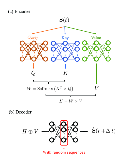
Figure 1: Schematic illustration of NANN’s architecture, which includes (a) encoder and (b) decoder. The encoder encodes the input $\mathbf{S}(t)$ into key $K$, query $Q$, and value $V$, leading to an attention weight $W$ and further to a state latent variable $H$. This compresses the input data sequence into a latent space representation while capturing intricate relationships within the sequence. The state latent variable $H$ can then be decoded by the decoder, where random sequences are introduced into every fully-connected layer to match the influences from stochastic noise. After training via minimizing the moment loss function $l$ that estimates the difference between the predicted state $\hat{\mathbf{S}}(t+\Delta t)$ and the target $\mathbf{S}(t+\Delta t)$, the predicted state $\hat{\mathbf{S}}(t+\Delta t)$ is expected to assume a similar probability distribution as the one obtained directly by the simulations. It is demonstrated in this work that NANN can learn to generate the long-term stochastic dynamics of the relatively larger system sizes by just training with the one-step dynamics on the relatively smaller system sizes. See text for more details.

The extrapolation of system size is another challenge that couples with the challenge of the stochastic noise. If a machine learning model can predict stochastic dynamics on relatively larger system sizes (assuming $N_{+}$ particles) by just training on the relatively smaller ones (assuming $N<N_{+}$ particles), it is then possible to accelerate the simulations in practice. For this purpose, before asking whether the stochastic dynamics of different system sizes can be generated effectively and efficiently, the machine learning model is required to be capable, at least in form, of flexibly dealing with multi system sizes. Ordinary feedforward architectures are not naturally suitable in this context (Goodfellow et al., 2016), and we shall focus on the network architectures with attention (Vaswani et al., 2017). The so-called attention is the key to the famous transformer architectures, which is also increasingly being applied to assisting physical investigations (Alkin et al., ; Geneva and Zabaras, 2022; Xu et al., 2024; Wu et al., ). It generally enables the machine learning model to flexibly deal with multi system sizes.

Incorporating these, we establish the noise-aware neural network (NANN) that combines a self-attention block (Vaswani et al., 2017) within the encoder (Sutskever et al., 2014), enabling the compression of the input data sequence into a latent space representation while capturing intricate relationships within the sequence. The decoder is composed of several fully-connected layers (Goodfellow et al., 2016), augmented by introduced random sequences. Such a setup can produce distinct outputs for the same input, corresponding to the variations observed in relevant systems due to stochastic noise. The PReLU function $\textrm{PReLU}(x)\equiv\max(0,x)+a\min(0,x)$ (where $a$ is the learnable parameter) (He et al., 2015) is applied as the activation function (Goodfellow et al., 2016) since it allows the effective prediction of the distribution of state variables containing negative values. Each input sample for NANN is a certain state $\mathbf{S}(t)$ that includes all the $M$ state variables of all the $N$ particles of the system at time $t$, which is a tensor with dimension $\left[N,M\right]$. The data samples are first encoded through a fully-connected layer $\boldsymbol{x}\equiv\left(x_{1},x_{2},\cdots,x_{M}\right)^{T}$ with $M$ neurons, followed by passing the encoded input samples to the attention block in the encoder. In the attention block, the key $K$ and query $Q$ contain information that determines the strength of interactions of each particle in the system with respect to all other particles, thus outputting an attention weight $W$ with dimension $\left[N,N\right]$ that models the strength of interactions among all particles. The value $V$ retains the characteristics of the input samples and is intended to be combined with the weight matrix to update the state representation of the latent space of the particle. Eventually, the updated state representation of particles in the latent space is decoded by a decoder consisting of fully-connected layers containing random sequences, so as to obtain the predicted state $\hat{\mathbf{S}}(t+\Delta t)$.

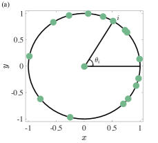
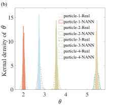
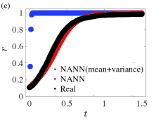
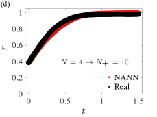
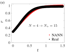
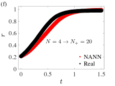
Figure 2: NANN based simulations on the noisy Kuramoto model. (a) Schematic illustration of the phase $\theta$ distribution of the noisy Kuramoto model consisting of $15$ limit-cycle oscillators for instance. (b) Direct comparison of the probability distribution of every oscillator’s phase in the subsequent time step concerning the noisy Kuramoto model’s one-step dynamics, with the solid lines corresponding to the NANN’s outcomes and the dashed lines corresponding to the results of the real simulations on this noisy Kuramoto model with $N=4$. (c) Direct comparison of the time evolution of the order parameter $r$ concerning the noisy Kuramoto model’s long-term stochastic dynamics, with the red markers corresponding to the NANN’s outcomes with $A=4$, the blue markers corresponding to the NANN’s outcomes with $A=2$, and the black markers corresponding to the results of the real simulations on this Vicsek model with $N=4$. Given only the $t=0$ one-step data for training, when only the first-order and second-order moments are taken into account in the moment loss function $l$, i.e., when $A=2$, the machine learning is completely unable to capture the physics. While in sharp contrast, the NANN trained with $A=4$ accomplishes its task very well. Furthermore, it successfully generates the long-term dynamics of the (d) $N_{+}=10$, (e) $N_{+}=15$, (f) $N_{+}=20$ systems by just training on $N=4$. See text for more details.

III NANN based simulation of the noisy Kuramoto model

To illustrate concretely how NANN can be applied in simulating stochastic dynamics, let us start with the noisy Kuramoto model (Acebrón et al., 2005; Rodrigues et al., 2016) as a preliminary demonstration. The physical system under consideration consists of $N$ limit-cycle oscillators with the presence of stochastic noise, whose dynamical equation reads (Acebrón et al., 2005; Rodrigues et al., 2016)

$$\dot{\theta_{i}}\left(t\right)=\omega_{i}+\eta_{i}\left(t\right)+\frac{J}{N}\sum_{j=1}^{N}\sin\left(\theta_{j}\left(t\right)-\theta_{i}\left(t\right)\right).$$ (2)

Here, $\eta_{i}(t)$ is a stochastic Gaussian noise, $\theta_{i}\left(t\right)$ is the phase of the $i$th oscillator, $\omega_{i}$ is its intrinsic natural frequency, and $J$ is a coupling strength. The phase coherence $r\equiv\langle\exp(i\theta(t))\rangle$ of all oscillators is a typical order parameter in this system, which reaches its maximum $r=1$ when all oscillators’ phases are synchronous, and its minimum $r=0$ when the phases are balanced around the circle, such as evenly spread or in clusters that balance each other out (Acebrón et al., 2005; Rodrigues et al., 2016). With all oscillators constrained to lie on the unit circle as illustrated in Fig. 2(a), the positions of every oscillator are determined by $x_{i}(t)\equiv\cos\theta_{i}(t),y_{i}(t)\equiv\sin\theta_{i}(t)$, and hence the phase $\theta_{i}\left(t\right)$ is the only state variable under consideration, i.e., $S_{i}(t)=\{\theta_{i}(t)\}$.

In this scenario, we train NANN with a series of known $\mathbf{S}(t)=\{S_{i}(t)\}$ ($i=1,2,\ldots,N$), and then let NANN predict the system’s state at $t+\Delta t$. This predicted state $\hat{\mathbf{S}}(t+\Delta t)$ is expected to hold the physical meaning of the possible phase configuration of all $N$ oscillators at $t$, and it shall be as similar as possible to the target $\mathbf{S}(t+\Delta t)$, i.e., the phase configuration obtained directly by the simulations. However, due to the target’s probabilistic changes driven by the stochastic noise, it is pointless to require the predicted phase for every $i$ and $t$ to be exactly the same as the one obtained directly by the simulations. Instead, when NANN learns the probability distribution that governs the generation of the target, one knows that its outputs actually simulate the dynamical equation under consideration, namely Eq. (2), and thus the time evolution of the order parameter $r$ shall be consistent between the one calculated using NANN’s outcomes and the one calculated using the results of the real simulations. We indeed find such results, as we shall see in the following.

Here, we fix $J=1$ and assume that every oscillator has the same $\omega_{i}=0.3$ for instance. The system is initialized to a typical state that the oscillator’s phase spans from $0$ to $2\pi$, and this initial state is provided to train the NANN, with any $t>0$ being a subsequent time step to be predicted. We first confirm that NANN can indeed learn the probability distribution that governs the generation of the target for the one-step evolution, as shown in Fig. 2(b). Then we examine its performance concerning the long-term dynamics. Fig. 2(c) shows a direct comparison of the time evolution of the order parameter $r$ for $N=4$ oscillators. The black curve is the $r$ calculated using the results of the real simulations. The blue curve is the $r$ calculated using NANN’s outcomes with $A=2$, i.e., it is trained with only the first-order moment (mean) and the second-order moment (variance). The red curve is the $r$ calculated using NANN’s outcomes with $A=4$.

From the blue curve in Fig. 2(c), one can clearly see that although the moment loss function $l$ provides a general framework for learning probability distributions, the powerful fitting ability of machine learning is completely unable to capture the physics when only the first-order and second-order moments are taken into account. This thus illustrates the technical difficulties of applying machine learning techniques to predicting and even accelerating stochastic dynamics simulations. Despite that, the NANN trained with $A=4$ predicts the stochastic dynamics simulations of this noisy Kuramoto model very well, as shown clearly in Fig. 2(c). The time evolution of the order parameter $r$ is highly consistent, manifesting that given only the $t=0$ one-step data for training, NANN has the effectiveness to predict the system’s state at arbitrary subsequent time steps.

Furthermore, NANN does not fixedly correspond to a specific particle number $N$, so it might have an extrapolation capability concerning the system size. Such an extrapolation is no doubt a non-trivial task, and its effectiveness needs to be examined in practice. But somewhat surprisingly, we find that NANN can indeed realize it very well. Fig. 2(d-f) shows the direct comparisons of the time evolution of the order parameter $r$ concerning different $N_{+}$. The black curves are the $r$ calculated using the results of the real simulations on $N_{+}=10,15,20$ systems, respectively. And the red curves are the $r$ calculated using NANN’s outcomes with $A=4$, just training on a relatively smaller $N=4$ system and then extrapolating to predict stochastic dynamics on the relatively larger $N_{+}=10,15,20$ systems, respectively. In a detailed check on the probability distributions of each particle, we confirm that extrapolating system size $N\rightarrow N_{+}$ does not break NANN’s effectiveness in learning the probability distribution. The consistency between NANN’s extrapolating outputs and the results of the real simulations is not only in the sense of ensemble average, but works for every particle at the same time. These results thus indicate that NANN can effectively deal with stochastic dynamics simulations, overcoming not only the challenge from the stochastic noise, but also the challenge from the extrapolation of system size.

IV Application of NANN in the flocking dynamics

In this section, let us switch to another prototypical but more complex model, namely the Vicsek model (Vicsek et al., 1995; Toner et al., 2005; Grégoire and Chaté, 2004; Chaté et al., 2008), to better demonstrate the effectiveness, efficiency, and generality of the NANN bashed approach in simulating stochastic dynamics. The physical system under consideration consists of $N$ self-propelled active particles in a two-dimensional box of size $L\times L$ with the presence of extrinsic stochastic noise, whose dynamical equation reads (Vicsek et al., 1995; Toner et al., 2005; Grégoire and Chaté, 2004; Chaté et al., 2008)

$$\boldsymbol{x}_{j}(t+\Delta t) =\boldsymbol{x}_{j}(t)+\boldsymbol{v}_{j}(t)\Delta t,$$ (3)

$$\theta_{j}(t+\Delta t) =\arg\sum_{k\in U_{j}}(e^{i\theta_{k}(t)}+\eta e^{i\xi_{j}(t)}).$$ (4)

Here, $\boldsymbol{x}_{j}(t)$, $\boldsymbol{v}_{j}(t)$ and $\theta_{j}(t)$ are the position, the velocity, and the direction of motion of the $j$th particle at time $t$, respectively. $\xi_{j}(t)\in[-\pi,\pi]$ is a uniformly distributed random noise with $\eta\in[0,1]$ being the extrinsic noise level. With all self-propelled particles assuming the same constant speed $v_{0}$, each particle adjusts its direction of motion in the time step based on the average velocity direction of all particles within its neighbors $U_{j}$ within a circular region of radius $R$. Concerning the flocking dynamics in this system, the group velocity $v_{a}=|\sum_{j=1}^{N}\boldsymbol{v}_{j}|/(Nv_{0})$ of all self-propelled particles is a typical order parameter (Vicsek et al., 1995; Toner et al., 2005; Grégoire and Chaté, 2004; Chaté et al., 2008), which reaches its maximum $v_{a}=1$ when the particles form a flock with their directions of motion are all aligned, and its minimum $v_{a}=0$ when the directions of motion are totally random. Distinguishing from the global interactions involved in the noisy Kuramoto model, the alignment involved here in the Vicsek model acts locally, and is even trickier since at the macroscopic level it is not Newtonian but actually based on the intelligent communicating and decision-making of the active agents (Vicsek et al., 1995; Toner et al., 2005; Grégoire and Chaté, 2004; Chaté et al., 2008). Therefore, this is not only a typical scenario that can better demonstrate NANN, but also a practical application scenario where more intricate collective phenomena are expected to emerge at larger scales (Kürsten and Ihle, 2020), calling for the assistance of machine learning.

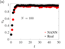
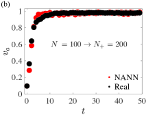
Figure 3: NANN’s application on simulations of flocking dynamics. (a) Direct comparison of the time evolution of the order parameter $v_{a}$ concerning the Vicsek model’s long-term flocking dynamics, with the red markers corresponding to the NANN’s outcomes and the black markers corresponding to the results of the real simulations on this Vicsek model with $N=100$. The consistency in $v_{a}$ manifests that, given only the $t=0$ one-step data for training, NANN has the effectiveness to predict this nonequilibrium complex system’s long-term dynamics. (b) The extrapolation capability of NANN in this scenario. NANN successfully generates the long-term dynamics of the $N_{+}=200$ system by just training on $N=100$. See text for more details.

In this scenario, $\boldsymbol{x}_{j}(t)$ and $\theta_{j}(t)$ are the state variables under consideration, i.e., $S_{j}(t)=\{\boldsymbol{x}_{j}(t),\theta_{j}(t)\}$. Using the moment loss function $l$ with $A=4$, we train NANN with a series of known $\mathbf{S}(t)=\{S_{j}(t)\}$ ($j=1,2,\ldots,N$), and then let NANN predict the system’s state at $t+\Delta t$. This predicted state $\hat{\mathbf{S}}(t+\Delta t)$ is expected to hold the physical meaning of the possible position and velocity configuration of all $N$ self-propelled particles at $t$, and it shall be as similar as possible to the target $\mathbf{S}(t+\Delta t)$, i.e., the position and velocity configuration obtained directly by the simulations. Here, we fix $\eta=0.2,L=5,R=1$ for instance, and assume periodic boundary conditions. The system is initialized in the disordered phase, and such random states are provided to train the NANN, with any $t>0$ being a subsequent time step to be predicted.

Fig. 3(a) shows a direct comparison of the time evolution of the order parameter $v_{a}$. The black curve is the $v_{a}$ calculated using the results of the real simulations on the $N=100$ system, and the red curve is the $v_{a}$ calculated using NANN’s outcomes for the same system size. The consistency in $v_{a}$ manifests that, given only the $t=0$ one-step data for training, NANN has the effectiveness to predict this nonequilibrium complex system’s long-term dynamics. In particular, the system’s long-term flocking dynamics appear quite differently and more complicatedly compared with the one-step evolution at $t=0$, but NANN’s effectiveness remains robust to a considerable extent. This can be expected only when the machine learning model does learn the underlying logic of Eq. (4), rather than merely learning specific patterns, configurations, or evolutionary trajectories. Furthermore, from Fig. 3(b) one can clearly see the extrapolation capability of NANN also remaining robust for this nonequilibrium complex system. NANN successfully generates the long-term dynamics of the $N_{+}=200$ system by just training on $N=100$. The time evolution of the group velocity $v_{a}$ of all $N$ self-propelled particles during the flocking dynamics reveal no considerable difference between NANN’s extrapolating outputs and the results of the real simulations on Eq. (4). These machine learning results for both the Vicsek model and the noisy Kuramoto model are obtained in a quite generic manner without any case-by-case special design on the network architecture, strongly suggesting that NANN can be readily applied for various complex systems.

In general, we find that the efficiency of using NANN to generate evolution trajectories can be about one order of magnitude higher than that of using the original algorithm to simulate the stochastic dynamics simulations on the same system size. On this foundation, when specifically applying NANN to any certain physical system, its efficiency can be further improved by providing more physical information to the machine learning model. Consider the noisy Kuramoto model for instance. Noticing that the interactions are global in that case, the attention weight $W$ in the architecture (see also Fig. 1) that models the strength of interactions among all particles can be set to unity by hand, which significantly improves the efficiency. Finally, it is worth mentioning that there of course exist some conventional but skillfully optimized algorithms that are even faster. It is common knowledge that artificial intelligence is currently unable to really master or even replace conventional human wisdom in physics. Like many machine learning applications in physics (Li et al., 2022; Behler and Parrinello, 2007; Chmiela et al., 2017; Zhang et al., 2018; Ko et al., 2019; Huang et al., 2021; Lu et al., 2021; He et al., 2022; Li et al., 2020; Xie et al., 2022, 2023; Carleo et al., 2019; Carrasquilla, 2020; Cichos et al., 2020; Carrasquilla and Melko, 2017; van Nieuwenburg et al., 2017; Li and Wang, 2018; Guo and He, 2023), NANN is a cooperator of those conventional ways, rather than a competitor. Taking the advantages of machine learning in terms of universality and transferability, NANN is intended to serve as a generic tool and help physicists more conveniently find the interesting physical systems and key parameter regions that are of special value and significance to be focused on and investigated in the conventional ways. In this practical sense, we believe that NANN can stimulate various investigations in all fields associated with stochastic dynamics simulations.

V Conclusions

We propose a new type of neural network, noise-aware neural network (NANN), based on which a generic machine learning approach is developed to simulate the stochastic dynamics, as demonstrated in the noisy Kuramoto model and the Vicsek model. A key feature of this approach is its ability to generate the long-term stochastic dynamics of complex large-scale systems by training NANN with the one-step dynamics of the smaller-scale systems. This can be particularly useful in investigating long-time dynamical behavior of large complex systems in different fields, ranging from active matter (Solon et al., 2015; Omar et al., 2021; Wysocki et al., 2014; Siebert et al., 2017; Digregorio et al., 2018; Speck, 2021; Fernandez-Rodriguez et al., 2020; Rein et al., 2023; Vicsek et al., 1995; Grégoire and Chaté, 2004; Toner et al., 2005; Chaté et al., 2008), over intelligent matter (Mosquera-Doñate and Boguñá, 2015; Rozanova and Boguñá, 2017; Yusufaly and Boedicker, 2016; Aguilar et al., 2021; Bäuerle et al., 2018; Zampetaki et al., 2021), to social physics (Farkas et al., 2003) and etc., where rich phenomena, such as the cross sea pattern of self-propelled particles (Kürsten and Ihle, 2020), the band pattern of self-propelled rods (Ginelli et al., 2010), and the large-scale vortex of moving microtubules (Sumino et al., 2012), etc., could emerge.