Emergence of entanglement and breakdown of causality in the quantum realm

Abstract

Entanglement is the most striking but also most weird property in quantum mechanics. It has been confirmed by many experiments over decades through the criterion of violating Bell’s inequality. However, a more fundamental problem arisen from EPR paradox is still not fully understood, that is, why quantum world emerges entanglement that classical physics does not. In this paper, we investigate the quantum dynamics of two photonic modes (or any two bosonic modes) coupled to each other through a beam splitting. Such a coupling fails to produce two-mode entanglement. We also start with a decoupled two-mode initial pure state, namely, no entanglement and no statistic feature to begin with. By solving the quantum equation of motion exactly without relying on the probabilistic interpretation, we find that when the initial wave function of one mode is different from a wave packet obeying minimum Heisenberg uncertainty (which corresponds to a well-defined classically particle), the causality in the time-evolution of another mode is broken down explicitly. It also leads to the emergence of quantum entanglement between the two modes. The lack of causality is the nature of statistics. The Bell’s inequality only excludes the possible existence of local hidden variables for the probabilistic interpretation of quantum mechanics. The internally causality breaking in the dynamical evolution of subsystems in isolated systems may answer the question how quantum dynamics generate naturally the probabilistic phenomena, even though the dynamical evolution of the whole system is completely described by the deterministic Schrödinger equation.

I Introduction

Quantum mechanics has been confirmed by countless experiments to be the most powerful theory for describing natural phenomena, but the nature of quantum mechanics itself has been the subject of debate and research since its inception. The most controversial issue is about the connection of the wave function solved from the deterministic Schrödinger equation to the physical quantities measured experimentally in reality. In particular, the statistical probability interpretation of the wave function which is very successful for all the measurement results in microscopic world, has rest the long historical debate begun with the two great physicists, Einstein and Bohr. In 1935, Einstein, Podolsky, and Rosen further pointed out that under the probability interpretation, quantum mechanical wave functions of distant noninteracting systems contain non-local correlations einstein1935can that goes far beyond the usual understanding of physical observations in reality. The non-local correlation feature of wave functions in composite systems was soon named as entanglement by Schrödinger schrodinger1935discussion , and becomes the most striking but also most weird property in quantum physics.

Over the past half century, numerous experiments have been developed to demonstrate the entanglement effects. The earliest experimental proof for EPR paradox, which was first recognized by Bohm and Aharonov bohm1957discussion , was indeed given in 1950 by Wu, et al. in their experiment of measuring the angular correlation of scattered annihilation photons Wu_PR_77 . It further inspired Bell to find mathematically an inequality for the correlations between two systems to be satisfied if there are local hidden variables associated with the probability description of measurement results bell1964einstein . Bell also showed that entanglement wave functions of distant noninteracting systems could violate this inequality. Thus, violation of Bell’s inequality becomes a criterion for demonstrating the non-local property of entanglement. Aspect aspect1982experimental ; aspect1982experimental' , Clauser clauser1969proposed ; freedman1972experimental , and Zeilinger weihs1998violation have been awarded the 2022 Nobel Prize in Physics for their groundbreaking experiments with entangled photons and pioneering the quantum information science. Nowadays, entanglement has become the most useful resource in quantum sciences for the development of quantum technologies.

Although the non-local property of entanglement has been well demonstrated by many experiments based on the violation of Bell’s inequality, a more fundamental question arisen from EPR paradox is, why and how entanglement emerges in the quantum world but not in classical physics? The non-locality (violation of Bell’s inequality) is a sufficient condition for the observation of entanglement between particles at a distant that any interaction between them can be ignored and excludes the possibility of having local hidden variables for quantum probabilistic description, but it does not answer the above question. Moreover, within the framework of the Standard Model which is build on the local gauge theory Weinberg2000 , non-local entanglements between various physical systems are all originally generated at an earlier time by more fundamental local interactions. For examples, photon-photon entanglements and electron-electron entanglements are indeed all generated through the local matter-photon interactions (or more fundamentally, QED). To date, there is no definite experimental evidence to show that the nature phenomena have gone beyond the predictions of the Standard Model. It remains an unsolved mystery why entanglement emerges only in the quantum world but not in classical physics.

On the other hand, for any entangled state of a composite system consisting of two or more subsystems, the reduced density matrix of subsystems represents a mixed state that cannot be expressed as a wave function that obeys the Schrödinger equation. That is, an entanglement state itself is governed by Schrödinger’s deterministic equation of motion but it produces internally a probabilistic description for its subsystem states. Apparently, such a description goes beyond the deterministic framework of the Schrödinger equation itself because probability phenomena are indeterministic, which is a natural consequence of the lack of causality in statistics. In response to the EPR paradox, Bohr had thought that it is the necessity of a final renunciation of the classical ideal of causality and a radical revision of our attitude towards the problem of physical reality add reference of Bohr . In this paper, we are going to show that the underlying feature of entanglement is indeed associated with the breakdown of causality for subsystem evolutions in composite systems, even though the Schrödinger equation is a deterministic equation of motion governing the dynamical evolution of the whole system. Thus, it is a big challenge to figure out, under what circumstances the causality would be broken down explicitly from a deterministic theory and meantime entangled states of composite systems emerge?

Without loss of the generality, we investigate in this paper the quantum dynamics of two photonic modes (or any two bosonic modes) coupled to each other through simple exchange transitions, such as beam splittings. Such coupling itself is unable to produce two-mode entanglement. We also start with a decoupled two-mode initial pure state, namely, no entanglement and no statistic feature to begin with. Then, we solve the deterministic quantum equation of motion exactly using the coherent state path integral approach ZhangRMP1990 ; Zhangbook2023 with some extensions TZ2008 ; JZ2010 ; LZ2012 ; LZ2018 ; Zhang2019 ; HZ2022b . Using the path integral approach is because the path integral formalism of quantum mechanics allows to make a direct connection between the quantum and classical deterministic dynamics and can show the explicit differences between quantum and classical physics. From such an investigation, we may unambiguously answer the key question explored in this work: why quantum world emerges the entanglement that classical physics does not? We find that it is different from classical dynamics, the causality in the quantum evolution for subsystems is broken down, and meantimes the entanglement between the two modes emerges. The lack of causality is also the nature of statistics, which further shows how the probabilistic feature of quantum states is manifested from the deterministic formulation of quantum mechanics itself.

II Coherent state path integrals formulation of quantum mechanics

In order to explore the origin of entanglement associated with the causality breaking so that the statistic feature of wave functions is manifested in the deterministic quantum equation of motion, we consider a very simple system consisting of a pair of photonic or more generally bosonic modes that couple to each other through simple exchange transitions. The system is described by the following simple Hamiltonian

$$H_{tot}=\hbar\omega_{1}a_{1}^{\dagger}a_{1}\!+\!\hbar\omega_{2}a_{2}^{\dagger}a_{2}\!+\!\hbar(V_{12}a_{1}^{\dagger}a_{2}\!+\!V^{\ast}_{12}a_{2}^{\dagger}a_{1}),$$ (1)

where $a_{1}^{\dagger}$ and $a_{2}^{\dagger}$ ($a_{1}$ and $a_{2}$) are the creation (annihilation) operators of the two photonic modes with frequencies $\omega_{1}$ and $\omega_{2}$, respectively. The last term in Eq. (1) describes the coupling of the two modes that can be easily realized with a beam splitting in experiments, for example. Because of the linearity, such a coupling fails to produce the two-mode entanglement. We will study the time-evolution of two modes governed deterministically by the Hamiltonian of Eq. (1). Also, two different initial states are specifically considered but both initial states are set to be separable pure states, namely there is also no entanglement and no statistic feature to begin with. Thus, the problem becomes very simple that anyone who has studied quantum mechanics can solve it. But using the path integral technique given in this paper, the exact solutions we obtained are surprising. It may resolve the fundamental issue in the long-running historical debate for quantum mechanics.

Specifically, we let mode 1 be initially in a coherent state (corresponding to a Gaussian wave packet with minimum Heisenberg uncertainty that can serve as a well-defined classical particle), the mode 2 can be initially either in a coherent state, or a squeezed state ZhangRMP1990 ; Zhangbook2023 . As it is well-known, photonic modes are one-to-one corresponding to harmonic oscillators. Within the framework of Schrödinger’s deterministic equation of motion, the time evolution of the coherent states for a single harmonic oscillator mode follows precisely the trajectories of an isolated classical harmonic oscillator for all kind of initial coherent states. This was originally discovered by Schrödinger in 1926 Sch_1926_WP and later developed by Glauber for quantum optics in 1963 glauber1963coherent , also see the review article by one of the author ZhangRMP1990 and the recent published book Zhangbook2023 . Thus, if mode 1 does not couple to mode 2, the quantum state will follows exactly the classical trajectories. With the above setups, we can examine physically in what conditions the quantum dynamics of the two modes can give rise to exactly the same classical dynamics, and under what circumstances the quantum dynamical will be deviated away from the classical dynamics such that the two modes evolve into an entangled state. We find that the time-evolution of the coupled two modes governed by the Hamiltonian of Eq. (1) with the two different initial states mentioned above behaves very different. The detailed calculations are given in Sec. III. Simply speaking, for the first case, the state of each mode keeps in a pure state at any later time, as one expected, because the coupling Hamiltonian of Eq. (1) cannot generate entanglement between the two modes. The corresponding quantum dynamical evolution follows exactly the classical trajectory solution. While, for the second case, the two modes will eventually entangled due to the squeezed state, as has been demonstrated in the quantum photonic circuit experiments, see for examples, Refs. QIC ; Zhong2020 ; Arrazola2021 . As a result, the state of each mode becomes a mixed state in the second case, the probabilistic feature and the entanglement between two modes are naturally emerges.

These results indicate that classical physics do not have entanglement. Entanglement generated from the deterministic equation of motion must accompany with the emergence of statistical probability for its subsystems. This implies that some fundamental law satisfied by classical deterministic dynamics should be broken down somewhere in the corresponding quantum evolution when entanglement emerges. We further find that this fundamental law is nothing but just the causality. To show explicitly this finding, we use the path integral technique in the coherent state representation ZhangRMP1990 ; Zhangbook2023 with some extensions TZ2008 ; JZ2010 ; LZ2012 ; LZ2018 ; Zhang2019 ; HZ2022b . This formulation can make a unambiguous quantum-to-classical correspondence ZhangPR95 . We then solve analytically and exactly the dynamics of the coupled two modes governed by Eq. (1) in terms of classical-like paths, to see where it has the possibility to break down the causality while the classical deterministic dynamics must obey.

Explicitly, the dynamics of the two modes is governed by the Schrödinger equation,

$$i\hbar\frac{d}{dt}|\psi_{tot}(t)\rangle=H_{tot}|\psi_{tot}(t)\rangle,$$ (2a)

or equivalently by the von Neumann equation

$$\dfrac{d}{dt}\rho_{tot}(t)=\dfrac{1}{i\hbar}[H_{tot},\rho_{tot}(t)],$$ (2b)

where $\rho_{tot}(t)=|\psi_{tot}(t)\rangle\langle\psi_{tot}(t)|$ is the density matrix of the two modes. If $|\psi_{tot}(t)\rangle$ is an entangled state, then the reduced density matrix $\rho_{1}(t)=\Tr_{2}[\rho_{tot}(t)]$ or $\rho_{2}(t)=\Tr_{1}[\rho_{tot}(t)]$ must be a mixed state, namely $\rho^{2}_{1}(t)\neq\rho_{1}(t)$ and $\rho^{2}_{2}(t)\neq\rho_{2}(t)$. Thus, it is more convenient (and indeed necessary) to begin with the von Neumann equation (2b) because Schrödinger equation is inconvenient (even not applicable for mixed states in principle). We will use the path integral technique to solve exactly the reduced density matrix $\rho_{1}(t)$ [or $\rho_{2}(t)$] from Eq. (2b) to see whether and how the entanglement emerges and how the causality is broken down, in terms of the same language used in the description of classical dynamics.

To be more specific, we focus on the dynamics of $\rho_{1}(t)$ which is obtained by the partial trace over the mode 2 states from the total density matrix of the two modes. The formal solution of Eq. (2b) for the total density matrix is given by

$$\rho_{tot}(t)=U(t,t_{0})\rho_{tot}(t_{0})U^{\dagger}(t,t_{0})$$ (3a)

with the time-evolution operator

$$U(t,t_{0})=\exp(-\frac{i}{\hbar}H_{tot}(t-t_{0})).$$ (3b)

For initially separable states of the two modes we will go to consider, the coherent state matrix element of $\rho_{1}(t)=\Tr_{2}[\rho_{tot}(t)]$ in terms of the path integrals can be expressed as TZ2008 ; JZ2010 ; LZ2012 ; LZ2018 ; Zhang2019 ; HZ2022b

$$\langle z_{1f}|\rho_{1}(t)|z^{\prime}_{1f}\rangle =\!\!\int\!d\mu(z_{1i})d\mu(z^{\prime}_{1i})\mathcal{J}(z_{1f},z^{\prime}_{1f},t;z_{1i},z^{\prime}_{1i},t_{0})$$

$$\qquad\qquad\qquad\times\!\langle z_{1i}|\rho_{1}(t_{0})|z^{\prime}_{1i}\rangle,$$ (4)

with the propagating function $\mathcal{J}(z_{1f},z^{\prime}_{1f},t;z_{1i},z^{\prime}_{1i},t_{0})$ defining as follows

$$\mathcal{J}(z_{1f}, z^{\prime}_{1f},t;~{}z_{1i},z^{\prime}_{1i},t_{0})$$

$$\equiv\!\!\int d\mu(z_{2i})d\mu(z^{\prime}_{2i})d\mu(z_{2f})\langle z_{1f}z_{2f}|U(t,t_{0})|z_{1i}z_{2i}\rangle$$

$$\!\times\!\langle z_{2i}|\rho_{2}(t_{0})|{z_{2i}}^{\prime}\rangle\langle z^{\prime}_{1i}z^{\prime}_{2i}|U^{\dagger}(t,t_{0})|z_{1f}z^{\prime}_{2f}\rangle$$

$$=B (z_{1},z^{\prime}_{1})\!\!\int\!e^{\frac{i}{\hbar}(S_{1}[z_{1}]-S_{1}^{\ast}[z^{\prime}_{1}])}F[z_{1},z^{\prime}_{1}]\mathcal{D}[z_{1}]\mathcal{D}[z^{\prime}_{1}].$$ (5)

Here all the dynamical effect of mode 2 on the mode 1 through simple exchange transitions is encompassed into the following influence functional, which was originally introduced by Feynman and Vernon Feynman1963 ,

$$F[z_{1},z^{\prime}_{1}] =\!\!\int\!d\mu^{\prime}(z_{1f})d\mu^{\prime}(z_{1i})d\mu^{\prime}({z_{1i}}^{\prime})\langle z_{2i}|\rho_{2}(t_{0})|{z_{2i}}^{\prime}\rangle$$

$$\!\times B(z_{2},z^{\prime}_{2})\!\!\int\!e^{\frac{i}{\hbar}(S_{2_{1}}[z_{1},z_{2}]-S^{\ast}_{2_{1}}[z^{\prime}_{1},z^{\prime}_{2}])}\mathcal{D}[z_{2}]\mathcal{D}[z^{\prime}_{2}].$$ (6)

The factor $B(z_{j},z^{\prime}_{j})=\exp(\Phi(z_{j})+\Phi^{\ast}(z^{\prime}_{j}))$ is the boundary effect in the coherent state path integral formulation with $\Phi(z_{j})=\frac{1}{2}{z^{\ast}_{jf}}z_{j}(t)+\frac{1}{2}z^{\ast}_{j}(t_{0})z_{ji}$ for $j=1,2$. This boundary factor was originally discovered by Feddeev and Slavnov in formulating the functional quantum field theory with a correct coherent state path integral formalism Faddeev1980 . The functions $S_{1}[z_{1}]$, $S_{2_{1}}[z_{1},z_{2}]$ are the classical actions of the two coupled photonic modes in the coherent state representation, coming straightforwardly from the forward time-evolution operator $U(t,t_{0})$ in path integrals,

$$S_{1}[z_{1}]=\!\!\int^{t}_{t_{0}}\!\!\Big{(}\frac{i\hbar}{2}(z^{\ast}_{1}\dot{z}_{1}-\dot{z}_{1}^{\ast}z_{1})-\hbar\omega_{1}z_{1}^{\ast}z_{1}\Big{)}d\tau,$$ (7a)

$$S_{2_{1}}[z_{1},z_{2}]=\!\!\int^{t}_{t_{0}}\!\!\Big{(}\frac{i\hbar}{2}(z^{\ast}_{2}\dot{z}_{2}-\dot{z}_{2}^{\ast}z_{2})-\hbar\omega_{2}z_{2}^{\ast}z_{2}$$

$$-\hbar V_{12}z^{\ast}_{1}z_{2}-\hbar V_{12}^{\ast}z_{2}^{\ast}z_{1}\Big{)}d\tau.$$ (7b)

The backward time-evolution operator $U^{\dagger}(t,t_{0})$ contributes the path integrals with the complex conjugate actions $S^{*}_{1}[z_{1}]$ and $S^{*}_{2_{1}}[z_{1},z_{2}]$ in Eqs. (II-II). Here, to avoid the unambiguous boundary conditions in coherent state path integral formalism ZhangRMP1990 ; Zhangbook2023 ; Schulman1981 ; Faddeev1980 , we have used the non-normalized coherent state $|z_{j}\rangle=\exp(z_{j}a^{\dagger}_{j})|0\rangle$ with the resolution of identity $\int|z_{j}\rangle\langle z_{j}|d\mu(z_{j})=1$, namely, the normalized factor is moved into the integral measure $d\mu(z_{j})=e^{-\absolutevalue{z_{j}}^{2}}\frac{dz^{\ast}_{j}dz_{j}}{2\pi i}$. The path integral measure $\mathcal{D}[z_{j}]=\prod_{t_{0}<\tau<t}d\mu(z_{j}(\tau))$. This completes the exact quantum mechanics formulation of the coupled two modes in terms of the coherent state path integrals for our further investigation. The formulation remains the same for much more complicated systems with slight extensions, see Refs. TZ2008 ; JZ2010 ; LZ2012 ; LZ2018 ; Zhang2019 ; HZ2022b .

III Solving the exact quantum dynamics with stationary paths

III.1 Stationary paths for quantum path integrals in bilinear systems

Path integral is defined as a sum over all possible paths (an infinity of quantum-mechanically possible paths) for the system evolving from one state to another. However, since the action shown by Eq. (7) is a quadratic function, only the stationary paths have the contribution to the path integral in Eqs. (II-II), which is always true for bilinear systems. The stationary paths obey the classical equations of motion determined by the least action principle $\delta S=0$. In other word, the stationary paths satisfy the Euler-Lagrange equation,

$$\frac{d}{d\tau}\frac{\partial\mathcal{L}}{\partial\dot{z}_{i}}-\frac{\partial\mathcal{L}}{\partial z_{i}}=0~{},~{}~{}\frac{d}{d\tau}\frac{\partial\mathcal{L}}{\partial\dot{z}^{*}_{i}}-\frac{\partial\mathcal{L}}{\partial z^{*}_{i}}=0.$$ (8)

This allows us to solve the quantum mechanics in terms of classical dynamics. It also provides a clean connection between the quantum and classical dynamics that can help us to answer the questions discussed in the introduction.

From Eq. (7b), we obtain the equations of motion for mode 2,

$$\frac{dz_{2}(\tau)}{d\tau}+i\omega_{2}z_{2}(\tau)+iV^{\ast}_{12}z_{1}(\tau)=0,$$ (9a)

$$\frac{dz^{\ast}_{2}(\tau)}{d\tau}-i\omega_{2}z^{\ast}_{2}(\tau)-iV_{12}z^{\ast}_{1}(\tau)=0.$$ (9b)

It is easy to check that with the transformation

$$z_{2}=\frac{1}{\sqrt{2}}(x_{2}+ip_{2})~{},~{}~{}z^{*}_{2}=\frac{1}{\sqrt{2}}(x_{2}-ip_{2})$$ (10)

where $x_{2}$ and $p_{2}$ are equivalent to the dimensionless position of momentum of the mode as a harmonic oscillator, Eq. (9) gives the exact classical equation of motion for mode 2 of the two coupled harmonic oscillators. On the other hand, Eq. (9b) is the conjugation of Eq. (9a). It is also a mathematical consequence that quantum evolution must obey the complex structure, arisen from the unitary evolution, just as the mathematical requirement of the symplectic structure for classical evolution of conservative systems ZhangRMP1990 ; ZhangPR95 ; Helgason1978 . Thus, quantum and classical evolution dynamics are unified in the same framework.

Not only these two equations of motion are conjugated to each other, their boundary conditions are also conjugated, i.e., the boundary conditions of Eqs. (9b) and (9a) are given by $z_{2}(t_{0})=z_{2i}$ and $z_{2}^{\ast}(t)=z_{2f}^{\ast}$, respectively. TZ2008 ; JZ2010 ; LZ2018 ; LZ2012 ; Zhang2019 . This is also a natural quantum mechanics result, namely, one cannot fixed the boundary condition of $z$ and $z^{*}$ (or equivalently the position and the momentum) at the same time, due to the uncertainty relationship. As a result, the solutions of these two equations of motion in Eq. (9) are given by,

$$z_{2}(\tau)=z_{2i}e^{-i\omega_{2}(\tau-t_{0})}-iV^{\ast}_{12}\!\!\int^{\tau}_{t_{0}}\!\!\!e^{-i\omega_{2}(\tau-\tau^{\prime})}z_{1}(\tau^{\prime})d\tau^{\prime},$$ (11a)

$$z_{2}^{\ast}(\tau)=z_{2f}^{\ast}e^{-i\omega_{2}(t-\tau)}-iV_{12}\!\!\int^{t}_{\tau}\!\!\!e^{-i\omega_{2}(\tau^{\prime}-\tau)}z^{\ast}_{1}(\tau^{\prime})d\tau^{\prime},$$ (11b)

where $t_{0}\leq\tau\leq t$, which agrees with the condition for unitary evolution. Equation (11) describes the full dynamics of mode 2 for the forward quantum evolution in Eq. (II). Likewise, we can find the stationary paths of mode 2 for the backward quantum evolution, i.e. the solution of the variables $z^{\prime}_{2}(\tau)$ and ${z^{\prime}_{2}}^{\ast}(\tau)$ from the stationary path equation of motion,

$$z^{\prime}_{2}(\tau)=z_{2f}e^{i\omega_{2}(t-\tau)}+iV^{\ast}_{12}\!\!\int^{t}_{\tau}\!\!\!e^{i\omega_{2}(\tau^{\prime}-\tau)}z_{1}(\tau^{\prime})d\tau^{\prime},$$ (12a)

$$z^{\prime\ast}_{2}(\tau)=z^{\prime\ast}_{2i}e^{i\omega_{2}(\tau-t_{0})}+iV_{12}\!\!\int^{\tau}_{t_{0}}\!\!\!e^{i\omega_{2}(\tau-\tau^{\prime})}z^{\prime\ast}_{1}(\tau^{\prime})d\tau^{\prime}.$$ (12b)

Thus, the path integrals in Eq. (II) is completely determined by the stationary paths given by Eqs. (11) and (12).

Remarkably, when we substitute the above solutions into Eq. (II) and completely integrate out the degrees of freedom of mode 2, the effect of mode 2 on the dynamics of mode 1 could be very different for different initial states of mode 2. To see the exact dynamical effect of mode 2 on mode 1, namely, to calculate the rest integrals in Eq. (II), we need to specify the initial states $|\psi_{tot}(t_{0})\rangle$ of the system. As we have discussed in Sec. II, we shall choose a separable initial state of the two modes so that no entanglement begins with:

$$|\psi_{tot}(t_{0})\rangle=|\alpha_{1}\rangle\otimes|\alpha_{2},s\rangle,$$ (13)

where $|\alpha_{1}\rangle=D(\alpha_{1})|0\rangle)$ is the usual coherent state and $|\alpha_{2},s\rangle=D(\alpha_{2})S(s)|0\rangle$ is a squeezed coherent state. The displacement operator $D(\alpha_{i})=\exp(\alpha_{i}a^{\dagger}_{i}-\alpha^{\ast}_{i}a_{i})$ with ($i=1,2)$ and the squeezed operator $S(s)=\exp(\frac{1}{2}(s^{\ast}a^{2}_{2}-s{a^{\dagger}}^{2}_{2}))$. The coherent parameters $\alpha_{i}$ and the squeezing parameter $s$ are complex numbers. We also rewrite the squeezing parameter as $s=\gamma e^{i\theta}$. Because Eq. (13) is a pure state, there is also no statistic feature to begin with. The two special initial states mentioned in Sec. II correspond to $s=0$ (i.e. $\gamma=0$) and $\alpha_{2}=0$, respectively. Namely, in the first initial state, two modes are both in coherent states, while in the second initial state, mode 1 is in a coherent state and mode 2 is in a squeezed state. Now, we go to show explicitly how the two different initial states of the mode 2 result in very different dynamical evolution of the mode 1.

In terms of the density matrix, the initial states of the mode 2 in Eq. (13) can be written as

$$\rho_{2}(t_{0})=|\alpha_{2},s\rangle\langle\alpha_{2},s|.$$ (14)

Thus, the influence functional Eq. (II) can be explicitly and exactly calculated. With the help of the faithful representation of the generalized Heisenberg group $H_{6}$, a subgroup of the symplectic group $Sp(4)$ ZhangRMP1990 , it is easy to find the functional functional Eq. (II),

$$F[z_{1},z^{\prime}_{1}]=\exp(\frac{i}{\hbar}S_{\rm eff}[z_{1},z^{\prime}_{1}]).$$ (15)

Here, $S_{\rm eff}[z_{1},z^{\prime}_{1}]$ denotes an effective action describing the dynamical effect of mode 2 on mode 1 through their coupling Hamiltonian in Eq. (1). Explicitly, the effective action is found to be

$$S_{\rm eff}[z_{1},z^{\prime}_{1}] =S_{\rm co}[z_{1},z^{\prime}_{1}]+S_{\rm sq}[z_{1},z^{\prime}_{1}]$$

$$+i\hbar\!\int^{t}_{t_{0}}\!\!d\tau\!\!\int^{\tau}_{t_{0}}\!\!\!d\tau^{\prime}\big{[}\chi^{*}_{1}({\tau})g(\tau,\tau^{\prime})z_{1}(\tau^{\prime})$$

$$\qquad\qquad\qquad-\!{z^{\prime}_{1}}^{\ast}(\tau^{\prime})g(\tau^{\prime},\tau)\chi_{1}({\tau})\big{]},$$ (16a)

where

$$S_{\rm co}[z_{1},z^{\prime}_{1}]= \!-\!\hbar V^{\ast}_{12}\alpha^{\ast}_{2}\!\!\int^{t}_{t_{0}}\!\!d\tau e^{i\omega_{2}(\tau-t_{0})}\chi_{1}({\tau})+\text{c.c.}$$ (16b)

$$S_{\rm sq}[z_{1},z^{\prime}_{1}]= \!-\!i\hbar\!\int^{t}_{t_{0}}\!\!d\tau\!\!\int^{t}_{t_{0}}\!\!\!d\tau^{\prime}\big{\{}\chi^{*}_{1}({\tau})\widetilde{g}(\tau,\tau^{\prime})\chi_{1}({\tau^{\prime}})$$

$$\qquad+\frac{1}{2}[\chi^{*}_{1}({\tau})\overline{g}(\tau,\tau^{\prime})\chi^{*}_{1}({\tau^{\prime}})+c.c.]\big{\}}$$ (16c)

are the contributions arisen from the coherent part and the squeezing part of the initial state in Eq. (14), respectively. We have also introduced the variable $\chi_{1}({\tau^{\prime}})=z_{1}(\tau^{\prime})\!-\!{z^{\prime}_{1}}(\tau^{\prime})$ which characterizes the difference between the forward and the backward paths for the density matrix evolution. The three two-time correlation functions in Eq. (16) are given by

$$g(\tau,\tau^{\prime}) =\absolutevalue{V_{12}}^{2}e^{-i\omega_{2}(\tau-\tau^{\prime})},$$ (17a)

$$\widetilde{g}(\tau,\tau^{\prime}) =\sinh^{2}\!\gamma\absolutevalue{V_{12}}^{2}e^{-i\omega_{2}(\tau-\tau^{\prime})},$$ (17b)

$$\overline{g}(\tau,\tau^{\prime}) =\frac{\sinh(2\gamma)e^{i(\theta+2\omega_{2}t_{0})}}{4}(V_{12})^{2}e^{-i\omega_{2}(\tau+\tau^{\prime})},$$ (17c)

which describe the two-time correlations between the two modes. Equation (16) shows that the coherence part in mode 2 initial state acts as a linear driving field applying on mode 1, see Eq. (16b). While the squeezing part induces non-local time correlations between the forward and backward evolutions of the reduced density matrix for mode 1, see Eq. (16c), which are indeed the sources for the breakdown of the causality as well as the emergence of entanglement, as we will show explicitly next.

III.2 Internally breakdown of causality and emergence of quantum entanglement

Having the exact analytical solution of the influence functional Eq. (II) given by Eqs. (15)-(16), we can now solve the propagating function Eq. (II) to determine the reduced density matrix of mode 1. Substituting Eq. (16) into Eq. (II), the classical action of the mode 1 in the path integrals is modified as $S_{1}[z_{1}]-S^{\ast}_{1}[z^{\prime}_{1}]+S_{\rm eff}[z_{1},z^{\prime}_{1}]$, where $S_{1}[z_{1}]$ is the classical action of mode 1 for the forward evolution, $S^{\ast}_{1}[z^{\prime}_{1}]$ is that of the backward evolution, and $S_{\rm eff}[z_{1},z^{\prime}_{1}]$ is the effective action induced by mode 2 on mode 1 through the two-mode coupling in Eq. (1), which mixes the forward and backward paths together. Note that the total action for the mode 1 is still a quadratic function of the complex variables $z_{1}$ and $z^{\prime}_{1}$. Thus, the path integrals of Eq. (II) are again fully determined by the stationary paths which obey the Euler-Lagrange equation governed by the action $S_{1}[z_{1}]-S^{\ast}_{1}[z^{\prime}_{1}]+S_{\rm eff}[z_{1},z^{\prime}_{1}]$. The resulting equations of motion for mode 1 are

$$\dot{z}_{1}(\tau)\!+\!i\omega_{1}z_{1}(\tau)\!+\!\!\!\int^{\tau}_{t_{0}}\!\!\!\!g(\tau,\tau^{\prime})z_{1}(\tau^{\prime})d\tau^{\prime}=\!-iV_{12}e^{-i\omega_{2}(\tau-t_{0})}\alpha_{2}$$

$$\qquad\!+\!\!\int^{t}_{t_{0}}\!\!\!\big{[}\overline{g}(\tau,\tau^{\prime})\chi^{*}_{1}({\tau^{\prime}})\!-\!\widetilde{g}(\tau,\tau^{\prime})\chi_{1}({\tau^{\prime}})\big{]}d\tau^{\prime},$$ (18a)

$$\dot{z}_{1}^{\ast}(\tau)\!-\!i\omega_{1}z_{1}^{\ast}(\tau)\!-\!\!\!\int^{t}_{\tau}\!\!\!g^{\ast}(\tau,\tau^{\prime})z_{1}^{\ast}(\tau^{\prime})d\tau^{\prime}\!=\!iV^{\ast}_{12}e^{i\omega_{2}(\tau-t_{0})}\alpha_{2}^{\ast}\!$$

$$\!-\!\!\int^{t}_{t_{0}}\!\!\!\big{\{}g^{\ast}(\tau,\tau^{\prime}){z^{\prime}_{1}}^{\ast}(\tau^{\prime})\!+\!\overline{g}^{\ast}(\tau,\tau^{\prime})\chi_{1}({\tau^{\prime}})\!-\!\widetilde{g}^{\ast}(\tau,\tau^{\prime})\chi^{*}_{1}({\tau^{\prime}})\big{]}d\tau^{\prime},$$ (18b)

$$\dot{z}^{\prime}_{1}(\tau)+i\omega_{1}z^{\prime}_{1}(\tau)\!-\!\!\!\int^{t}_{\tau}\!\!\!g(\tau,\tau^{\prime})z^{\prime}_{1}(\tau^{\prime})d\tau^{\prime}\!=\!-iV_{12}e^{-i\omega_{2}(\tau-t_{0})}\alpha_{2}$$

$$\!-\!\!\int^{t}_{t_{0}}\!\!\!\big{[}g(\tau,\tau^{\prime})z_{1}(\tau^{\prime})\!-\!\overline{g}(\tau,\tau^{\prime})\chi^{*}_{1}({\tau^{\prime}})\!+\!\widetilde{g}(\tau,\tau^{\prime})\chi_{1}({\tau^{\prime}})\big{]}d\tau^{\prime},$$ (18c)

$${\dot{z}_{1}}^{\prime\ast}\!(\tau)\!-\!i\omega_{1}{z^{\prime}_{1}}^{\ast}\!(\tau)\!+\!\!\!\int^{\tau}_{t_{0}}\!\!\!\!g^{\ast}(\tau,\tau^{\prime}){z^{\prime}_{1}}^{\ast}\!(\tau^{\prime})d\tau^{\prime}\!=iV^{\ast}_{12}e^{i\omega_{2}(\tau-t_{0})}\alpha_{2}^{\ast}$$

$$\qquad-\!\!\int^{t}_{t_{0}}\!\!\!\big{[}\overline{g}^{\ast}(\tau,\tau^{\prime})\chi_{1}({\tau^{\prime}})\!-\!\widetilde{g}^{\ast}(\tau,\tau^{\prime})\chi^{*}_{1}({\tau^{\prime}})\big{]}d\tau^{\prime},$$ (18d)

subjected to the boundary conditions $z_{1}(t_{0})=z_{1i}$, $z^{\ast}_{1}(t)=z^{\ast}_{1f}$, $z^{\prime}_{1}(t)=z^{\prime}_{1f}$ and ${z^{\prime}_{1}}^{\ast}(t_{0})={z^{\prime}_{1i}}^{\ast}$, where $t_{0}\leq\tau\leq t$. Because $\chi_{1}({\tau^{\prime}})=z_{1}(\tau^{\prime})\!-\!{z^{\prime}_{1}}(\tau^{\prime})$, Eq. (18) shows that the forward and backward paths are all mixed together. Combining the solutions of Eq. (18) with the solutions of Eqs. (11)-(12) for mode 2, it shows that the forward and backward paths of mode 2 are mixed as well. As one can see, Eqs. (18a) and (18b) [also Eqs. (18c) and (18d)] are no longer conjugated each other. In other words, we start with a unitary evolution formulation for the two-mode coupling system but the unitary evolution is broken down when we look at the dynamical evolution of each mode. This is indeed a general consequence for open quantum systems, namely for any composite quantum system (a system consists of two or more subsystems), the dynamical evolution of each individual quantum subsystem must be non-unitary TZ2008 ; JZ2010 ; LZ2012 ; LZ2018 ; Zhang2019 ; HZ2022b .

Moreover, these equations of motion in Eq. (18), which determine all the contributions for the path integrals Eq. (II), show that not only the quantum unitary evolution is broken down, the causality of its dynamical evolution is also broken down for each mode, even though these equations are derived from the deterministic evolution equation Eq. (2b) without taking any approximation. Explicitly, Eq. (18a) shows that the solution of the forward path $z_{1}(\tau)$ at time $\tau$ evolves from $t_{0}$ to $\tau$, but it is also affected by its future dynamics from $\tau$ to $t$, see the last term in Eq. (18a). This is an explicit breakdown of the causality manifested through the classical-type equations of motion. Likewise, Eq. (18c) shows again that the backward path at time $\tau$ evolves from $t$ to $\tau$, but is also influenced by its later dynamics from $\tau$ to $t_{0}$. The other two equations of motion for their conjugate variables, i.e., Eqs. (18b) and (18d), show the same property of the breakdown of the causality, and meantimes also show the breakdown of the unitary. Here, the breakdown of unitary means that the equations of motion for the variable $z_{1}(\tau)$ and $z^{*}_{1}(\tau)$ are no longer conjugated each other. As it is shown, the breakdown of causality only occurs for each mode rather than for dynamics of two mode as a whole. Therefore, we called such kind of causality breaking as an internally causality breaking. Due to the breakdown of causality, finding the corresponding solutions of these equations of motion is usually not an easy task.

However, using the approach we have developed in solving the dynamics of open quantum systems in the last two decades TZ2008 ; JZ2010 ; LZ2012 ; LZ2018 ; Zhang2019 ; HZ2022b , the mixed forward and backward paths with the causality breaking can actually be solved analytically. This is done by introducing a formal solution (a linear transformations) to Eq. (18),

$$z_{1}(\tau)=u(\tau,t_{0})z_{1i}+v_{0}(\tau,t_{0})\alpha_{2}$$

$$\qquad\quad-v_{1}(\tau,t)\chi(t)-v_{2}(\tau,t)\chi^{*}(t),$$ (19a)

$${z^{\prime}_{1}}^{\ast}(\tau)=u^{\ast}(\tau,t_{0}){z^{\prime}}^{\ast}_{1i}+v_{0}^{\ast}(\tau,t_{0})\alpha^{\ast}_{2}$$

$$\qquad\qquad+v^{\ast}_{1}(\tau,t)\chi^{*}(t)+v^{\ast}_{2}(\tau,t)\chi(t),$$ (19b)

$$\chi(\tau)=u^{\ast}(t,\tau)\chi(t),~{}~{}\chi^{*}(\tau)=u(t,\tau)\chi^{*}(t)$$ (19c)

where $\chi(t)=z_{1}(t)-z^{\prime}_{1f}$ and $\chi^{*}(t)=z^{\ast}_{1f}-{z^{\prime}}^{\ast}_{1}(t)$, and $z_{1}(t)$ and ${z^{\prime}}^{\ast}_{1}(t)$ are the end point values of the stationary paths that can be self-consistently determined from the above solution, while $z^{\prime}_{1f}$ and $z^{\ast}_{1f}$ are the end point values in formulating the path integrals, see Eq. (II). With the above transformation, the equations of motion Eq. (18) are reduced to

$$\dot{u}(\tau,t_{0})+i\omega_{1}u(\tau,t_{0})+\!\int^{\tau}_{t_{0}}\!\!g(\tau,\tau^{\prime})u(\tau^{\prime},t_{0})d\tau^{\prime}\!=\!0,$$ (20a)

$$\dot{v}_{0}(\tau,t_{0})+i\omega_{1}v_{0}(\tau,t_{0})+\!\int^{\tau}_{t_{0}}\!\!g(\tau,t^{\prime})v_{0}(t^{\prime},t_{0})dt^{\prime}$$

$$~{}~{}~{}~{}~{}~{}~{}~{}~{}~{}~{}~{}~{}~{}~{}~{}~{}~{}~{}~{}~{}~{}~{}~{}~{}~{}~{}=\!-iV_{12}e^{-i\omega_{2}(\tau-t_{0})},$$ (20b)

$$\dot{v}_{1}(\tau,t)+i\omega_{1}v_{1}(\tau,t)+\!\int^{\tau}_{t_{0}}\!\!g(\tau,\tau^{\prime})v_{1}(\tau^{\prime},t)d\tau^{\prime}$$

$$~{}~{}~{}~{}~{}~{}~{}~{}~{}~{}~{}~{}~{}~{}~{}~{}~{}~{}~{}~{}~{}~{}~{}~{}~{}~{}~{}=\!\int^{t}_{t_{0}}\!\!\widetilde{g}(\tau,\tau^{\prime})u^{*}(t,\tau^{\prime})d\tau^{\prime},$$ (20c)

$$\dot{v}_{2}(\tau,t)+i\omega_{1}v_{2}(\tau,t)+\!\int^{\tau}_{t_{0}}\!\!g(\tau,\tau^{\prime})v_{2}(\tau^{\prime},t)d\tau^{\prime}$$

$$~{}~{}~{}~{}~{}~{}~{}~{}~{}~{}~{}~{}~{}~{}~{}~{}~{}~{}~{}~{}~{}~{}~{}~{}~{}~{}~{}=\!-\!\int^{t}_{t_{0}}\!\!\overline{g}(\tau,\tau^{\prime})u(t,\tau^{\prime})d\tau^{\prime},$$ (20d)

subjected to the boundary conditions: $u(t_{0},t_{0})=1$, $v_{0}(t_{0},t_{0})=0$, $v_{1}(t_{0},t)=0$ and $v_{2}(t_{0},t)=0$. These time-correlation functions correspond indeed to the nonequilibrium Green functions as we have shown in solving the general dynamics of open quantum systems TZ2008 ; JZ2010 ; LZ2012 ; LZ2018 ; Zhang2019 ; HZ2022b . The analytical solution of these nonequilibrium Green functions can be easily obtained:

$$u(\tau,t_{0}) =\cos^{2}(\frac{\varphi}{2})e^{-i\omega_{+}(\tau-t_{0})}+\sin^{2}(\frac{\varphi}{2})e^{-i\omega_{-}(\tau-t_{0})},$$ (21a)

$$v_{0}(\tau,t_{0}) =-iV_{12}\int^{\tau}_{t_{0}}\!\!u(\tau,\tau_{1})e^{-i\omega_{2}(\tau_{1}-t_{0})}d\tau_{1},$$ (21b)

$$v_{1}(\tau,t) =\!\int^{\tau}_{t_{0}}\!\!d\tau_{1}\int^{t}_{t_{0}}\!\!d\tau_{2}u(\tau,\tau_{1})\widetilde{g}(\tau_{1},\tau_{2})u^{\ast}(t,\tau_{2}),$$

$$=\sinh^{2}\gamma v(\tau,t_{0})v^{*}(t,t_{0})$$ (21c)

$$v_{2}(\tau,t) =-\!\!\int^{\tau}_{t_{0}}\!\!d\tau_{1}\int^{t}_{t_{0}}\!\!d\tau_{2}u(\tau,\tau_{1})\overline{g}(\tau_{1},\tau_{2})u(t,\tau_{2})$$

$$=\frac{1}{4}\sinh(2\gamma)e^{i\theta}v(\tau,t_{0})v(t,t_{0}),$$ (21d)

where $\omega_{\pm}=\frac{1}{2}(\omega_{1}+\omega_{2})\pm\frac{1}{2}\sqrt{[(\omega_{1}-\omega_{2})]^{2}+4\absolutevalue{V_{12}}^{2}}$ and $\varphi=\tan^{-1}(\frac{2\absolutevalue{V_{12}}}{\omega_{1}-\omega_{2}})$.

Equations (19) and (21) gives the exact analytical solution of the stationary paths determined by the equations of motion of Eq. (18). The causality breaking is shown explicitly in these solutions. For example, the solution of the forward path $z_{1}(\tau)$ given by Eq. (19a) contains four terms. The first two terms [$\sim u(\tau,t_{0})$ and $v_{0}(\tau,t_{0})$] are arisen from its past historical motion with the coupling to the motion of another mode. The last two terms [$\sim v_{1}(\tau,t)$ and $v_{2}(\tau,t)$] are contributed from its future motion mixing with the backward stationary paths. Such kind of solutions should not occur in the classical deterministic evolution alone because of the causality. We find further that the above causality breaking occurs only if the squeezing parameter in the initial state of the mode 2 does not vanish, i.e., $s\neq 0$ in Eq. (13).

If $s=0$, i.e. $\gamma=0$ so that both modes are initially in coherent states, see Eq. (13), then the two-time correlations $\widetilde{g}(\tau,\tau^{\prime})=0$ and $\overline{g}(\tau,\tau^{\prime})=0$, see Eq. (17). This directly leads to $v_{1}(\tau,t)=0$ and $v_{2}(\tau,t)=0$, as shown by Eqs. (21c) and (21d). As a result, Eq. (19) is reduced to

$$z_{1}(\tau)=u(\tau,t_{0})z_{1i}+v_{0}(\tau,t_{0})\alpha_{2},$$ (22a)

$${z^{\prime}_{1}}^{\ast}(\tau)=u^{\ast}(\tau,t_{0}){z^{\prime}}^{\ast}_{1i}+v_{0}^{\ast}(\tau,t_{0})\alpha^{\ast}_{2},$$ (22b)

which shows that the causality is recovered. In other words, if the initial states of both modes are coherent states, they correspond to wave packets with the minimum uncertainty $\Delta x=\Delta p$ and $\Delta x\Delta p=1/2$). In this situation, the causality maintains in quantum dynamical evolution of the coupled two modes. Note that the wave packets with minimum Heisenberg uncertainty have been described and defined as classical particles. The solution of Eq. (22) fully agrees with the classical solution, namely, the quantum evolution of coherent states can reproduce the exact classical dynamics of the two coupled harmonic oscillators.

However, if $\gamma\neq 0$, i.e., the initial state of mode 2 is a coherent squeezed state, which contains pure quantum effect (squeezing) that goes beyond the properties of a classical particle, then $v_{1}(\tau,t)\neq 0$ and $v_{2}(\tau,t)\neq 0$ such that the causality of the stationary paths for each mode is no longer preserved, as shown by the solution of Eq. (19) with Eq. (21). Thus, it is the quantumness in the initial state of mode 2 induces the influence of the future dynamics ($t>\tau$) of mode 1 on its present dynamics at $\tau$ so that the causality is broken down. We find further that the about internally causality breaking, i.e., all the stationary paths are determined by their past as well as their future dynamics for each mode, indeed accompanies with the emergence of entanglement between the two modes, even though the two modes are initially unentangled and the coupling of the two modes given in Eq. (1) cannot generates entanglement. To make this conclusion explicitly, we are now going to solve the reduced density matrix $\rho_{1}(t)$ for mode 1.

Using the equations of motion Eq. (18), the propagating function Eq. (II) can be simply reduced to

$$\mathcal{J}(z_{1f} ,z^{\prime}_{1f},t;z_{1i},z^{\prime}_{1i},t_{0})\!=\!\bar{N}(t)\exp\!\Big{\{}\!\frac{1}{2}\big{[}z^{\ast}_{1f}z_{1}(t)\!+\!z^{\ast}_{1}(t_{0})z_{1i}$$

$$+\!{z^{\prime}_{1}}^{\ast}(t)z^{\prime}_{1f}\!+\!{z^{\prime}}^{\ast}_{1i}z^{\prime}_{1}(t_{0})\!+\!(z^{\ast}_{1f}\!-\!{z^{\prime}_{1}}^{\ast}(t))v_{0}(t,t_{0})\alpha_{2}$$

$$\!-\!\alpha^{\ast}_{2}v_{0}^{\ast}(t,t_{0})(z_{1}(t)\!-\!z^{\prime}_{1f})\big{]}\!\Big{\}},$$ (23)

where $\bar{N}(t)$ represents the fluctuations around the stationary paths but it is only a simple time-dependent factor that can be determined by the fact $\Tr[\rho_{tot}(t)]=1$, see the next. The end-point values of the stationary paths $z_{1}(t)$, $z^{\ast}_{1}(t_{0})$, $z^{\prime}_{1}(t_{0})$ and ${z^{\prime}_{1}}^{\ast}(t)$ can be obtained from Eq. (19). With the solution of the propagating function, and the initial state $\rho_{1}(t_{0})=|\alpha_{1}\rangle\langle\alpha_{1}|$ given in Eq. (13), we find the analytical reduced density matrix $\rho_{1}(t)$ of mode 1 in the coherent state representation

$$\langle z_{1f}|\rho_{1}(t)|z^{\prime}_{1f}\rangle= N(t)\exp\{z_{1f}^{\ast}\alpha(t)\!-\!\frac{1}{2}\beta(t)(z_{1f}^{\ast}\!-\!\alpha^{\ast}(t))^{2}\Big{\}}$$

$$\times\exp\left\{\delta(t)(z_{f}^{\ast}\!-\!\alpha^{\ast}(t))(z^{\prime}_{f}\!-\!\alpha(t))\right\}$$

$$\times\exp\{\alpha^{\ast}(t)z^{\prime}_{1f}\!-\!\frac{1}{2}\beta^{*}(t)(z^{\prime}_{1f}\!-\!\alpha(t))^{2}\Big{\}}$$ (24)

where $\alpha(t)=u(t,t_{0})\alpha_{1}+v_{0}(t,t_{0})\alpha_{2}$, and

$$\begin{split}&\beta(t)=\frac{\tanh\gamma e^{i\theta}v_{0}^{2}(t,t_{0})}{1-(1-\absolutevalue{v_{0}(t,t_{0})}^{2})^{2}\tanh^{2}\gamma}\\ &\delta(t)=\frac{\tanh^{2}\gamma(1-\absolutevalue{v_{0}(t,t_{0})}^{2})\absolutevalue{v_{0}(t,t_{0})}^{2}}{1-(1-\absolutevalue{v_{0}(t,t_{0})}^{2})^{2}\tanh^{2}\gamma}\\ &N(t)=\frac{\sech\gamma\exp(-\absolutevalue{\alpha(t)}^{2})}{\sqrt{1-(1-\absolutevalue{v_{0}(t,t_{0})}^{2})^{2}\tanh^{2}\gamma}}.\end{split}$$ (25)

In Eq. (III.2), the term $\delta(t)(z_{2f}^{\ast}-\beta^{\ast}(t))(z^{\prime}_{2f}-\beta(t))$ in the middle exponent factor or more precisely, the term $\delta(t)z_{2f}^{\ast}z^{\prime}_{2f}$ in the exponent makes the reduced density matrix impossible to be written as the external product of a pure state. In other words, $\rho_{1}(t)$ must be a mixed state if the coefficient $\delta(t)$ is not zero. On the other hand, the total density matrix of the two modes must maintain in a pure state under the quantum evolution governed by Eq. (1) because the initial state of Eq. (13) is a pure state and the total system is isolated. This is equivalently to say that the total state of this coupled two-mode system has become a pure entanglement state during the dynamical evolution, it cannot be written as a direct product of the two individual mode states, namely $\rho_{tot}(t)\neq\rho_{1}(t)\otimes\rho_{2}(t)$ if $\gamma\neq 0$.

More explicitly, we can write down the exact reduced density operator $\rho_{1}(t)$ from Eq. (III.2) without relying on the coherent state representation,

$$\rho_{1} (t)=\tilde{N}e^{A^{\dagger}(t)}\bigg{[}\sum^{\infty}_{n=0}\delta^{n}(t)|n\rangle\langle n|\bigg{]}e^{A(t)}$$ (26)

with $\tilde{N}\!=\!N\exp(\delta(t)\absolutevalue{\alpha(t)}^{2}\!-\!\frac{1}{2}(\beta^{*}(t)\alpha(t)^{2}\!+\!\beta(t)\alpha^{*}(t)^{2}))$, $A^{\dagger}(t)\!\equiv\![(1\!-\!\delta(t))\alpha(t)\!+\!\beta(t)\alpha^{*}(t)]a^{\dagger}_{1}\!-\!\frac{1}{2}\beta(t)a^{{\dagger}2}_{1}$, and $|n\rangle=\frac{1}{\sqrt{n!}}(a^{\dagger}_{1})^{n}|0\rangle$ is the Fock state. The summation $\sum^{\infty}_{n=0}\delta^{n}(t)|n\rangle\langle n|$ is indeed a thermal-like state when $\delta(t)$ is not zero. Thus, the state $\rho_{1}(t)$ is obviously a mixed state. We can also re-express the reduced density matrix $\rho_{1}(t)$ as

$$\rho_{1}(t)=\mathcal{N}\sum^{\infty}_{n=0}\frac{\delta^{n}(t)}{n!}(a^{\dagger}_{1})^{n}|\tilde{\alpha}(t),\xi(t)\rangle\langle\tilde{\alpha}(t),\xi(t)|(a_{1})^{n},$$ (27)

where $|\tilde{\alpha}(t),\xi(t)\rangle$ is a squeezed coherent state. The coherent parameter $\tilde{\alpha}(t)=\frac{1}{1-\absolutevalue{\beta(t)}^{2}}(c^{\ast}(t)-\beta(t)c(t))$ and $\xi(t)=\bar{\gamma}e^{i\bar{\theta}}$ ($\bar{\gamma}=\frac{1}{2}\ln\frac{1-\absolutevalue{\beta(t)}}{1+\absolutevalue{\beta(t)}}$ and $\bar{\theta}\!=\!\arg(\beta(t)^{\ast}/2)$), and $c(t)\!=\!(1-\delta(t))\alpha^{\ast}(t)+\beta^{*}(t)\alpha(t)$. In fact, Eqs. (26) and (27) are usually called as squeezed thermal state or thermalized squeezing state.

The reason that the reduced density matrix $\rho_{1}(t)$ of mode 1 becomes a mixed state (i.e. the two modes are entangled) through their dynamical evolution is because the initial state of mode 2 contains quantumness. If mode 2 is initially also in a coherent state as mode 1, namely both modes are initially in coherent states corresponding to minimum-uncertainty wave packets for well-defined classical particles, the reduced density matrix $\rho_{1}(t)$ will keep to stay in pure states (more precisely, coherent states), and the entanglement between the two modes never emerge. This can be easily justified by setting the squeezed parameter $s_{2}=0$ (i.e., $\gamma=0$) in the initial state of Eq. (13). This setting immediately leads to the coefficients $\beta(t)=0$ and $\delta(t)=0$ in Eq. (25). Thus, the reduced density matrix $\rho_{1}(t)$ in Eq. (III.2), (26) and (27) is simply reduced to

$$\rho_{1}(t)=D(\alpha(t))|0\rangle\langle 0|D^{\dagger}(\alpha(t))=|\alpha(t)\rangle\langle\alpha(t)|,$$ (28)

where $\alpha(t)=u(t,t_{0})\alpha_{1}+v_{0}(t,t_{0})\alpha_{2}$. This is a pure state and evolves exactly as a classical harmonic oscillator, no entanglement emerges. It describes precisely the same evolution of a classical harmonic oscillator with the trajectory given by $\alpha(t)$ in the complex phase space, where the causality is preserved, which agrees with the solution of Eq. (22). This also answers the question why classical physics does not exist entanglement, and the causality is well preserved.

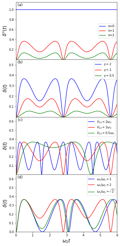
Figure 1: (Colour online) The dimensionless coefficient $\delta(t)$ in Eq. (III.2)-(27) as a function of time, which characterizes the mixing degree of the reduced density matrix $\rho_{1}(t)$. (a) The first few terms in the expansion of Eq. (26), $\delta^{n}(t)$ with $n=0,1,2$, the other parameters in the calculation are $(\omega_{1}/\omega_{2})=2$, $V_{12}=\omega_{2}$, and the squeezed parameter $\gamma=2$. (b-d) $\delta(t)$ for different squeezed parameter $\gamma=2,1,0.5$, the different coupling strength parameters $V_{12}=(2,1,0.5)\omega_{2}$, and the different frequencies setting $(\omega_{1},\omega_{2})=(1,1),(2,1),(\sqrt{2},1)$, respectively.

To see how the reduced density matrix $\rho_{1}(t)$ changes in time as a mixed state, which is characterized by $\delta(t)\neq 0$ when $\gamma\neq 0$, we present some numerical results in Fig. 1 for the values of $\delta(t)$ in time for various different cases. In Fig. 1(a) we show the first few values of $\delta^{n}(t)$ in the expansion of Eq. (26) [or Eq. (27)]. It shows that the mixed state of mode 1 (also representing the entanglement between the two modes) change periodically in time. It becomes more clear in Fig. 1(b-d), where $\delta(t)$ is plotted as a function of time for the different squeezed parameters, different coupling strengths, and different set of the two mode frequencies, respectively. It always shows the periodicity, which is the essence for finite quantum systems. As long as the system contains finite number of particles or modes, the evolution is always periodic. The squeezing strength $\gamma$ affects the oscillation amplitude, as shown in Fig. 1(b). The two-mode coupling strength $V_{12}$ changes the oscillation frequencies, as given by Fig. 1(c), which corresponding to the two normal mode frequencies in Eq. (21a). Because of the periodicity, there is still a discrete set of points that $\delta(t)=0$ where the states of both modes retrieve to be a pure state and no entanglement occurs at these points, but the measure of the set is zero. In the reality, many other modes exist in the surrounding, different frequencies will generate different normal mode frequencies which causes different periodicities, as shown in Fig. 1(d). Thus, when one oscillator couples to many other modes, the periodicities of $\delta(t)$ will be eventually merged and disappear. This is in fact a general procedure of how a subsystem in a complicated composite system is eventually thermalized HZ2022 , even though the initial system of the total system is a pure state here. The underlying feature behind the thermalization is indeed the internally causality breaking for every part of a large composite system. This is the foundation of statistical mechanics and thermodynamics. We will leave this problem in a further investigation YZ2024 .

IV Discussions and Perspectives

In this paper, we study the physical underpinning of the entanglement emergence from the quantum evolution of a coupled two-mode system, a very simple system that can be easily implemented and demonstrated experimentally. The coupling is linear, so it does not inherently create entanglement between the two modes. We also start with separable initial pure states of the two modes, so there are no entanglement and also no statistic feature to begin with. In particular, we set one mode initially in a Glauber coherent state which is a wave packet with minimum uncertainty ($\Delta x=\Delta p$ and $\Delta x\Delta p=\hbar/2$) that is one-to-one corresponding to a classical particle in a harmonic potential. Thus, by looking at the deterministic quantum evolution governed by the coupled Hamiltonian Eq. (1), we have shown in what conditions the Glauber coherent state can give rise to exactly the same classical dynamics, and under what circumstances it will tune to be a mixed state so the two modes evolve into an entangled state. Such an investigation provides the way to explore the essence and the origin of the entanglement in quantum realm. We find that the emergence of entanglement is accompanied with the internally causality breaking, and both stem from the quantumness containing in the initial state (in this paper we used the squeezed state) of another mode. If another mode is also initially in a Glauber coherent state, no entanglement emerges and causality does not be broken in the dynamical evolution of each mode. The corresponding quantum dynamics gives rise precisely the same classical dynamics of the two coupled harmonic oscillators. This answers to some extent the question of why entanglement emerges in the quantum world that cannot occur in classical physics.

The system and the setting studied in this paper are simple but quite unique. This is because the Glauber coherent states (wave packets with minimal Heisenberg uncertainty) are the only quantum states that behave as classical particles that can evolve exactly along their classical trajectories in a harmonic potential. It provides a unique way to distinguish the differences between quantum and classical dynamics in terms of the same language and to demonstrate quantum properties that are not present in classical physics. In the seminal EPR paper einstein1935can , Einstein et al. proposed the thought experiment of using a plane-wave wavefunction to describe the entanglement between particles at a distant that the interaction between them can be ignored. It is a thought experiment because a plane-wave wavefunction is quantum mechanically unphysical Tannoudji1991 , the corresponding probability is equally distributed in the space and the overall probability is divergent so experimental measurements for such physical particles are infeasible. David Bohm reformulated the EPR experiment later by considering a pair of entangled spin-$1/2$ particles that can be measured Bohm1951 . But a spin system (or more generally, fermionic systems) is intrinsically a quantum system that differs from classical systems. In fact, any system containing two or a few finite states has no direct correspondence with a classical system. It is difficult, if not impossible, to find other systems and setups whose quantum dynamics can exactly reproduce the corresponding classical dynamics on the one hand ZhangPR95 ; Zhang1990 ; Zhang1994 , and on the other hand, demonstrate quantum properties not present in classical physics, by simply changing the initial states.

Although the system and setups in this paper are very simple and quite unique, the conclusion we obtained is actually general. The exact solution of the reduced density matrix of mode 1 solved from the deterministic evolution equation of the two-mode coupling system can be straightforwardly extended to many-mode coupling systems, including continuously distributed infinite modes. As long as the coupling is bilinear, and the initial states of other modes are not all in the coherent states, entanglement inevitably emerges. The emergence of entanglement is accompanied by the internally causality breaking in the dynamical evolution of each mode, as manifested through the same equations of motion of Eq. (18), with slightly changing the two-time correlations of Eq. (17) to a summation over all other modes. This formulation has been shown in our general investigations to open quantum system dynamics LZ2012 ; HZ2022b . The further extension to many-fermionic systems is also straightforward, by changing the complex variables to the Grassmann variables in the same equations of motion for the stationary paths with some sign changes caused by the anti-exchange property of Grassmann variables TZ2008 ; JZ2010 . Thus, emergence of entanglement accompanying with the internally causality breaking is manifested in the same ways in fermionic systems. In fact, this is a general consequence for any composite systems, the emergence of entanglement between two or more subsystems always accompanies by the breakdown of causality in the dynamical evolution of these subsystems, except for linear coupling bosonic systems with all particles being initially in wave packets with minimum Heisenberg uncertainty. This is because the final solutions from the equations of motion obtained in this paper are determined by Eq. (20), which corresponds to the basic nonequilibrium Green functions that can be easily extended to any many-body quantum systems and quantum field theory, where different interactions will result in different but more complicated two-time correlations between different subsystems than that given by Eq. (17) Zhang2019 .

As an extension, the rigorous and exact solution obtained from the simple composite system in this paper shows that the breakdown of the causality generally occurs for subsystems. This is why we called it as an internally causality breaking. While, the evolution of the whole systems (i.e., isolated systems) follows the deterministic Schrödinger equation. It should be true that the quantum dynamical evolution of various constitutes in isolated systems all breaks internally the causality. Schrödinger equation is the quantum equation of motion for isolated systems only. Any constitute in a physical system cannot be treated as an isolated system, even for the single electron in hydrogen atom. As an illustration, the electron in atoms must interact with nucleus to form the bound states and it also interacts with photons to give the transitions between different states. Therefore, electron and its movement is only a part of the quantum dynamics of atoms, molecules and solids. Our solution indicates that the causality in the quantum evolution of every electron should be internally broken, even though the electron paths would be more complicated than the example we studied in this paper and cannot be determined by stationary paths alone in the path integrals. More importantly, the internally causality breaking naturally leads to a probabilistic description for all quantum measurements, because when the system is measured, it is no longer an isolated system. Consequently, it is hard to see precisely the movement of single electron in atoms, molecules and solids, even though some dynamical effects of single electron have been observed by means of the attosecond spectroscopy Krausz2010 ; LHuillier2017 ; Krausz2009 ; Agostini2014 . It should not be possible to track the electron (and any particle) movement when it transits between different states, not because of the very short timescales but due to the internally causality breaking for various particles in quantum realm. The lack of causality is the nature of statistics. This may reveal the long-standing mystery why quantum mechanics holds a probabilistic interpretation. It is the internally causality breaking in quantum dynamics makes the measurement results become probabilistic.

At last, one might ask how such internally causality breaking in quantum systems can be detected experimentally. To a certain extent, it requires to detect the advanced-time effect rather than the retarded-time effect in the dynamical evolution, which is far more than just a difficulty. State-of-the-art experimental setups are needed. The advanced experimental technologies, such as precision measurement or non-demolition measurements Thorne1980 ; Haroche2007a ; Haroche2007b and the faster detection with attosecond spectroscopy Krausz2009 ; Agostini2014 may be useful. Nevertheless, we show that the internally causality breaking in quantum systems is the inherent property of quantum mechanics. It opens up a new avenue to explore many related fundamental physics problems that have not been fully understood so far, such as the foundation of thermalization in nature, the dynamical evolution of bio-systems, and even the origin of our universe, etc. It may also provide a new direction for the development of quantum technology. As one knows, the main obstacle for the development of quantum technology comes from the inevitable decoherence effect. From our previous research on decoherence theory TZ2008 ; Zhang2012 ; LZ2018 ; HZ2022b , one can see that decoherence stems from the same reason as the emergence of entanglement and probability in quantum systems, i.e., the internally causality breaking. Therefore, instead of devoting huge resources to overcome the inevitable decoherence effects raised by the environment as well as the manipulations of quantum states (it also has the same problem for topological states LZ2018 ; HZ2020 ) for performing quantum computational unitary operations, it may be a more promising direction for attempting to compatibly combine and utilize the characteristics of entanglement, decoherence and probabilities together towards achieving new breakthroughs in quantum technology. We leave these researches for further investigations.

- (1) A. Einstein, B. Podolsky, and N. Rosen, Can quantum- mechanical description of physical reality be considered complete?, Phys. Rev. 47, 777 (1935).
- (2) E. Schrödinger, Discussion of probability relations be- tween separated systems, Mathematical Proceedings of the Cambridge Philosophical Society, 31, 555 (1935).
- (3) D. Bohm and Y. Aharonov, Discussion of experimental proof for the paradox of Einstein, Rosen, and Podolsky, Phys. Rev. 108, 1070 (1957).
- (4) C. S. Wu and I. Shaknov, The angular correlation of scattered annihilation radiation, Phys. Rev. 77, 136 (1950)
- (5) J. S. Bell, On the Einstein Podolsky Rosen paradox, Physics Physique Fizika 1, 195 (1964).
- (6) A. Aspect, P. Grangier, and G. Roger, Experimental realization of Einstein-Podolsky-Rosen-Bohm Gedankenexperiment: A new violation of bell’s inequalities, Phys. Rev. Lett. 49, 91 (1982).
- (7) A. Aspect, J. Dalibard, and G. Roger, Experimental test of Bell’s inequalities using time-varying analyzers, Phys. Rev. Lett. 49, 1804 (1982).
- (8) J. F. Clauser, M. A. Horne, A. Shimony, and R. A. Holt, Proposed experiment to test local hidden-variable theories, Phys. Rev. Lett. 23, 880 (1969).
- (9) S. J. Freedman and J. F. Clauser, Experimental test of local hidden-variable theories, Phys. Rev. Lett. 28, 938 (1972).
- (10) G. Weihs, T. Jennewein, C. Simon, H. Weinfurter, and A. Zeilinge, Violation of Bell’s inequality under strict Einstein locality conditions, Phys. Rev. Lett. 81, 5039 (1998).
- (11) S. Weinberg, The Quantum Theory of Fields, Vol. I: Foundations (Cambridge Univ. Press, UK, 1995).
- (12) N. Bohr, Can quantum-mechanical description of physical reality be considered complete?, Phys. Rev. 48, 696 (1935).
- (13) W. M. Zhang, D. H. Feng, and R. Gilmore, Coherent states: Theory and some applications, Rev. Mod. Phys. 62, 867 (1990).
- (14) C. F. Kam, W. M. Zhang, and D. H. Feng, Coherent States: New Insights into Quantum Mechanics with Applications. Lecture Notes in Physics (Springer-Verlag, 2023).
- (15) M. W. Y. Tu and W. M. Zhang, Non-Markovian decoherence theory for a double-dot charge qubit, Phys. Rev. B 78, 235311 (2008).
- (16) J. Jin, M. W. Y. Tu, W. M. Zhang, and Y. J. Yan, Non-equilibrium quantum theory for nanodevices based on the Feynman-Vernon influence functional, New J. Phys. 12, 083013 (2010).
- (17) C. U. Lei and W. M. Zhang, A quantum photonic dissipative transport theory, Ann. Phys. 327, 1408 (2012).
- (18) H. L. Lai, P. Y. Yang, Y. W. Huang, and W. M. Zhang, Exact master equation and non-Markovian decoherence dynamics of Majorana zero modes under gate-induced charge fluctuations, Phys. Rev. B 97, 054508 (2018).
- (19) W. M. Zhang, Exact master equation and general non-Markovian dynamics in open quantum systems, Eur. Phys. J. Special Topics on Non-equilibrium Dynamics: Quantum Systems and Foundations of Quantum Mechanics, 227, 1849 (2019).
- (20) Y. W. Huang and W. M. Zhang, Exact master equation for generalized quantum Brownian motion with momentum-dependent system-environment couplings, Phys. Rev. Res. 4, 033151 (2022).
- (21) E. Schrödinger, Der stetige Übergang von der Mikro-zur Makromechanik, Naturwiss. 14, 664–666 (1926).
- (22) R. J. Glauber, Coherent and incoherent states of the radiation field, Phys. Rev. 131, 2766 (1963).
- (23) A. Politi, J. C. F. Matthews, M. G. Thompson, and J. L. O’Brien, Integrated quantum photonics, IEEE J. Quantum Electron. 15, 1673–1684 (2009).
- (24) H.-S. Zhong, H. Wang, Y.-H. Deng, M. C. Chen, L.-C. Peng, Y.-H. Luo, J. Qin, D. Wu, X. Ding, […], and J.-W. Pan. Quantum computational advantage using photons. Science 370, 1460 (2020).
- (25) J. M. Arrazola, V. Bergholm, K. Brádler, T. R. Bromley, M. J. Collins, I. Dhand, A. Fumagalli, T. Gerrits, A. Goussev, L. G. Helt, et al., Quantum circuits with many photons on a programmable nanophotonic chip, Nature (London) 591, 54 (2021).
- (26) W. M. Zhang and D. H. Feng, Quantum nonintegrability in finite systems, Phys. Rep. 252, 1 (1995).
- (27) R. P. Feynman and F. L. Vernon, The theory of a general quantum system interacting with a linear dissipative system, Ann. Phys. 24, 118 (1963).
- (28) L. D. Faddeev and A. A. Slavnov, Gauge Fields: Introduction to Quantum Theory (Benjamin-Cummings, Reading, MA, 1980).
- (29) S. L. Schulman, Techniques and Applications of Path Integration (Wiley, New York, 1981).
- (30) S. Helgason, Differential Geometry, Lie Groups and Symmetric Space (Academic, New York, 1978).
- (31) W. M. Zhang, P. Y. Lo, H. N. Xiong, M. W. Y. Tu, and F. Nori, General Non-Markovian Dynamics of Open Quantum Systems, Phys. Rev. Lett. 109, 170402 (2012).
- (32) W. M. Huang and W. M. Zhang, Nonperturbative renormalization of quantum thermodynamics from weak to strong couplings, Phys. Rev. Research 4, 023141(2022).
- (33) S. K. Yang and W. M. Zhang, The dynamical foundation of statistical mechanics and thermalization, (in preparation, 2024).
- (34) C. Cohen-Tannoudji, B. Diu, and F. Laloe, Quantum Mechanics,1st ed. (Wiley, New York, 1977).
- (35) D. Bohm, Quantum Theory, (Prentice-Hall, Inc., New Jersey, 1951).
- (36) W. M. Zhang, J. M. Yuan, D. H. Feng, Q. Pan, and J. Tjon, Quantum fluctuations in classical chaos, Phys. Rev. A 40, R3646 (1990).
- (37) I. Zlatev, W. M. Zhang, and D. H. Feng, Possibility that Schrödinger’s conjecture for the hydrogen-atom coherent states is not attainable, Phys. Rev. A 50, R1793 (1994).
- (38) M. Schultze, M. Fiess, N. Karpowics, J. Gagnon, M. Korbman, M. Hofstetter, S. Neppl, A. L. Cavalieri, Y. Komninos, Th. Mercouris, C. A Nicolaides, R. Pazourek, S. Nagele, J. Feist, J. Burgdörfer, A. M. Azzeer, R. Ernstorfer, R. Kienberger, U. Kleineberg, E. Goulielmakis, F. Krausz and V. S. Yakovlev, Delay in Photoemission, Science 328, 1658 (2010).
- (39) M. Isinger, R.J. Squibb, D. Busto, S. Zhong, A. Harth, D. Kroon, S. Nandi, C.L. Arnold, M. Miranda, J.M. Dahlström, E. Lindroth, R Feifel, M. Gisselbrecht and A. L’Huillier, Photoionization in the time and frequency domain, Science 358, 893 (2017).
- (40) F. Krausz and M. Ivanov, Attosecond physics, Rev. Mod. Phys. 81, 163 (2009).
- (41) S. Ghimire, G. Ndabashimiye, A. D. DiChiara, E. Sistrunk, M. I Stockman, P. Agostini, L. F. DiMauro and D. A. Reis, Strong-field and attosecond physics in solids, J. Phys. B: At. Mol. Opt. Phys. 47, 204030 (2014).
- (42) V. B. Braginsky, Y. I. Vorontsov, and K. S. Thorne, Quantum Non-demolition Measurements, Science, 209, 547 (1980).
- (43) S. Gleyzes, S. Kuhr, C. Guerlin, J. Bernu, S. Deléglise, U. Busk Hoff, M. Brune, J. M. Raimond and S. Haroche, Quantum jumps of light recording the birth and death of a photon in a cavity, Nature 446, 297 (2007).
- (44) C. Guerlin, J. Bernu, S. Deléglise, C. Sayrin, S. Gleyzes, S. Kuhr, M. Brune, J.M. Raimond and S. Haroche, Progressive field-state collapse and quantum non-demolition photon counting, Nature 448, 889 (2007).
- (45) Y. W. Huang, P. Y. Yang, and W. M. Zhang, Quantum theory of dissipative topological systems, Phys. Rev. B 102, 165116 (2020).