Delay Dispersion in IRS-assisted FSO Links

Abstract

The line-of-sight (LOS) requirement of free-space optical (FSO) systems can be relaxed by employing optical intelligent reflecting surfaces (IRSs). In this paper, we model the impact of the IRS-induced delay dispersion and derive the channel impulse response (CIR) of IRS-assisted FSO links. The proposed model takes into account the characteristics of the incident and reflected beams’ wavefronts, the position of transmitter and receiver, the size of the IRS, and the incident beamwidth on the IRS. Our simulation results reveal that a maximum effective delay spread of 0.7 ns is expected for a square IRS with area 1 $\mathrm{m}^{2}$, which induces inter-symbol interference for bit rates larger than 10 Gbps. We show that the IRS-induced delay dispersion can be mitigated via equalization at the receiver.

I Introduction

Free space optical (FSO) systems are prime candidates for incorporation in next generation wireless communication networks [1]. Due to their directional narrow laser beams, easy-to-install transceivers, and high data rates, FSO links are appealing for last-mile access, fiber backup, and backhaul of wireless networks. The line-of-sight (LOS) requirement of FSO systems can be relaxed by employing optical relays or optical intelligent reflecting surfaces (IRSs) [2]. Optical IRSs are planar structures which can change the properties of the incident beam such as its phase and polarization [3, 4, 5].

The authors in [6, 7, 8] have developed deterministic and statistical channel models for IRS-assisted FSO links. Based on these models, they analyzed the impact of IRSs on the normalized received power, known as geometric loss, and the misalignment loss due to random movements of the transmitter (Tx), IRS, and receiver (Rx). Moreover, in [5, 9], the authors studied the impact of the IRS size and phase shift profile on the received power at the Rx lens and compared the end-to-end performance with that achieved with optical relays.

Optical IRSs can be implemented as planar surfaces equipped with arrays of micro-mirrors or meta-material-based passive subwavelength elements [10, 11]. The former technology uses specular reflection by adjusting the orientation of the micro-mirrors to redirect the incident beam in the desired direction. In contrast, metamaterial-based IRSs change the phase of the incident beam locally at every IRS element and provide anomalous reflection to point the beam towards the desired direction. Thus, for both types of IRSs, every IRS element reflects part of the beam incident on the IRS. The parts of the beam reflected by different IRS elements have different distances to the Rx lens. Depending on the size of the beam footprint on the IRS, the size of the IRS, and the position of Tx and Rx, the different delays experienced by different parts of the reflected beam may cause IRS-induced channel dispersion. Moreover, due to the high data rate of FSO links (typically on the order of 1-10 Gbps), the symbol duration is very small (0.1 - 1 ns). Thus, the delay dispersion introduced by the IRS may cause inter-symbol interference (ISI), which degrades the end-to-end performance and needs to be mitigated. The authors in [12] investigated the impact of the time delay between different antenna elements of a phased array and the resulting ISI for wideband millimeter-wave signals. Moreover, the authors in [13] studied the frequency domain characteristics of IRS-assisted visible light communication (VLC) and the corresponding achievable rate. However, to the best of the authors’ knowledge, the IRS-induced channel dispersion of FSO links has not been investigated in the literature, yet.

In this paper, we analyze the delay dispersion caused by IRS-assisted FSO links given the phase profile of the transmitted and reflected beams. Then, we derive the channel impulse response (CIR) using the Huygens-Fresnel principle where we take into account the size of the IRS and the positions of Tx and Rx. Furthermore, we mitigate the channel dispersion-induced ISI using digital equalization methods. Our simulation results reveal that the delay spread introduced by the IRS elements increases with the difference between the angle of the incident beam and the angle of the reflected beam on the IRS, denoted by $\Delta\theta$. Moreover, as $\Delta\theta$ increases, the channel gain decreases due to the higher geometric loss of the IRS-assisted FSO link. Furthermore, we show that for dispersive FSO channels equalization can greatly improve performance.

II System and Channel Models

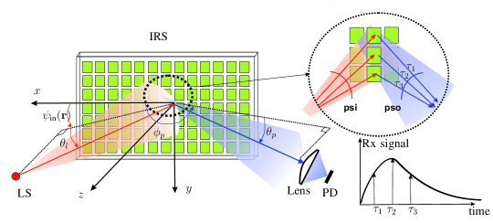
Figure 1: IRS-assisted FSO system model.

We consider a point-to-point FSO link, where the Tx is equipped with a laser source (LS) and connected via an optical IRS to a Rx, which is equipped with a photo detector (PD) and a lens, see Fig. 1. The $xy$-plane of the adopted $xyz$-coordinate system coincides with the IRS plane and the center of the IRS is in the origin.

II-A System Model

II-A1 Transmitter

The Tx is equipped with an LS emitting a Gaussian laser beam. The beam axis intersects with the $xy$-plane at distance $d_{l}$ and points in direction $\mathbf{\Psi}_{l}=\left(\theta_{l},\phi_{l}\right)$, where $\theta_{l}$ is the angle between the $xy$-plane and the beam axis, and $\phi_{l}$ is the angle between the projection of the beam axis on the $xy$-plane and the $x$-axis, see Fig. 1.

We consider the transmission of a sequence of independent and identically distributed (i.i.d.) symbols $a[m]$. After pulse shaping, the optical transmit signal is given by

$$s(t)={P_{0}}\sum_{m=-\infty}^{+\infty}a[m]g_{\text{tx}}(t-mT),$$ (1)

where ${P_{0}}$ is the transmit power, $a[m]\in\{0,1\}$ are on-off keying (OOK) modulated symbols, and $g_{\text{tx}}(t)$ is the real-valued pulse shaping filter with symbol duration $T$, see Fig. 2.

We assume rectangular pulses, which are easy to realize in FSO systems [14] and are defined as

$$g_{\text{tx}}(t)=\frac{1}{T}\Pi\left({\frac{t}{T}}\right),\quad$$ (2)

with spectrum $G_{\text{tx}}(f)=\int_{-\infty}^{\infty}g_{\text{tx}}(t)e^{-\mathrm{j}2\pi ft}\mathrm{d}t=\text{sinc}\left({T\pi f}\right)$. Here, $\text{sinc}(x)=\frac{\sin(x)}{x}$ is the sinc-function and $\Pi(\cdot)$ is defined as $\Pi(\frac{x}{a})=1$ for $|x|<\frac{a}{2}$ and $\Pi(\frac{x}{a})=0$ otherwise.

II-A2 Receiver

The Rx is equipped with a PD and a circular lens of radius $a$. The lens of the Rx is located at distance $d_{p}$ from the origin of the $xyz$-coordinate system. The normal vector of the lens plane points in direction $\mathbf{\Psi}_{p}=\left(\theta_{p},\phi_{p}\right)$, where $\theta_{p}$ is the angle between the $xy$-plane and the normal vector, and $\phi_{p}$ is the angle between the projection of the normal vector on the $xy$-plane and the $x$-axis.

We assume a direct detection system, where the PD produces an electrical current, $y(t)$, which is proportional to the optical power received at the lens, i.e., $y(t)=s(t)\circledast h(t)$, where $\circledast$ denotes the convolution. Moreover, $h(t)$ is the CIR in equivalent baseband representation which will be discussed in detail in Section II-B. Assuming that the PD has no bandwidth constraint, after filtering $y(t)$ with a receive filter $g_{\text{rx}}(t)$ matched to the transmit pulse, i.e., $g_{\text{rx}}(t)=g_{\text{tx}}^{*}(-t)$, the electrical signal $u(t)$ before sampling is given by

$$u(t) =\left({y}(t)+\tilde{n}(t)\right)\circledast g_{\text{rx}}(t)=r(t)+n(t),$$ (3)

where ${r}(t)=y(t)\circledast g_{\text{rx}}(t)$ [17, 14] and $(\cdot)^{*}$ denotes the complex conjugate operator. Furthermore, $\tilde{n}(t)$ is additive white Gaussian noise with mean zero and power spectral density $N_{0}$. The filtered noise $n(t)=\tilde{n}(t)\circledast g_{\text{rx}}(t)$ is a zero-mean Gaussian process with autocorrelation function $\frac{N_{0}}{2}\Phi_{{g_{\text{rx}}}{g_{\text{rx}}}}(\tau)$, where $\Phi_{{g_{\text{rx}}}{g_{\text{rx}}}}(\tau)=g_{\text{rx}}(\tau)\circledast g_{\text{rx}}^{*}(-\tau)$.

II-A3 IRS

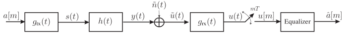
Figure 2: End-to-end optical system model.

The size of the IRS is $L_{x}\times L_{y}$ and it consists of $Q=Q_{x}Q_{y}$ subwavelength elements, where $Q_{x}$ and $Q_{y}$ are the numbers of elements in $x$- and $y$-direction, respectively. Given that the size of the IRS is much larger than the optical wavelength, i.e., $L_{x},L_{y}\gg\lambda$, the IRS can be modeled as a continuous surface with a continuous phase shift profile denoted by $\Phi_{\text{irs}}(\mathbf{r})$ [5], where $\mathbf{r}=[x,y]^{T}$ denotes a point in the $xy$-plane and $(\cdot)^{T}$ refers to transposition. The phase shift introduced by the IRS is exploited such that it compensates the phase difference between the incident and the desired beam. Given the positions of the LS, $\left(d_{l},\mathbf{\Psi}_{l}\right)$, and the PD, $\left(d_{p},\mathbf{\Psi}_{p}\right)$, we adopt a linear phase shift profile as follows [8]

$$\phi_{\text{irs}}(\mathbf{r}) =k\left(\Phi_{0}+\Phi_{x}x+\Phi_{y}y\right),\qquad$$ (4)

where $k=\frac{2\pi}{\lambda}$ is the wave number, $\lambda$ is the wavelength, $\Phi_{x}=\cos(\theta_{l})\cos(\phi_{l})+\cos(\theta_{p})\cos(\phi_{p})$, $\Phi_{y}=\cos(\theta_{l})\sin(\phi_{l})+\cos(\theta_{p})\sin(\phi_{p})$, and $\Phi_{0}$ is constant.

II-A4 Discrete-Time System Model

By sampling signal $u(t)$ at times $t=mT$ and defining $u[m]\overset{\Delta}{=}u(mT)$, we obtain

$$u[m] {=}\sum\limits_{\ell=-\infty}^{\infty}h_{e}[\ell]{a}[m-\ell]+n[m]$$ (5)

$$=h_{e}[0]{a}[m]+\sum_{\ell\neq m}h_{e}[\ell]{a}[m-\ell]+n[m],$$

where $h_{e}[m]\overset{\Delta}{=}h_{e}(mT)$ and $h_{e}(t)=h(t)\circledast g_{\text{tx}}(t)\circledast g_{\text{rx}}(t)$ is the overall impulse response. $n[m]=n(mT)$ has autocorrelation function $\Phi_{nn}[m]={N_{0}\over 2}\delta[m]$, i.e., the discrete-time noise is white. Here, $\delta[\cdot]$ denotes the Kronecker delta function. If the channel delay dispersion is negligible and there is no ISI in the channel, then, $h_{e}[m]=h_{\text{0}}\delta[m]$, where $h_{\text{0}}$ is a constant. This is the conventional system model for point-to-point non-dispersive FSO channels.

II-B Channel Model

IRS-assisted FSO channels are impaired by geometric and misalignment losses (GML), atmospheric loss, and atmospheric turbulence induced fading [8]. Thus, the CIR of the considered FSO system can be modeled as follows

$$h(t)=Rh_{p}h_{a}h_{\text{gml}}(t),\quad$$ (6)

where $R$ is the PD responsivity, $h_{a}$ represents the random atmospheric turbulence induced fading, $h_{p}$ is the atmospheric loss, and $h_{\text{gml}}(t)$ characterizes the GML impulse response.

In (6), to characterize the temporal characteristics of the IRS-assisted FSO channel, we ignore the delay dispersion due to atmospheric turbulence. In fact, it was shown in [18] that for typical data rates of FSO links, which are on the order of several Gbps and a link distance of 1 km, the root mean square (RMS) delay spread due to atmospheric turbulence is about 10 ps in rainy weather [18]. Given symbol durations on the order of 0.1 ns, the delay dispersion due to atmospheric turbulence is practically negligible [19].

On the other hand, the GML impulse response $h_{\text{gml}}(t)$ represents the normalized power collected at the lens disregarding the atmospheric loss and atmospheric turbulence and is given by [5]

$$h_{\text{gml}}(t)=\frac{1}{2\eta P_{0}}\int_{\mathcal{A}_{\text{lens}}}\lvert E_{\text{rx}}(\mathbf{r}_{p},t)\rvert^{2}\mathrm{d}\mathbf{r}_{p},$$ (7)

where $E_{\text{rx}}(\mathbf{r}_{p},t)$ is the received electric field at time $t$, $\eta$ is the free-space impedance, $\mathcal{A}_{\text{lens}}$ denotes the area of the Rx lens, and $\mathbf{r}_{p}=[x_{p},y_{p}]^{T}$ denotes a point in the lens plane. Here, the origin of the $x_{p}y_{p}z_{p}$-coordinate system is the center of the lens and the $z_{p}$-axis is parallel to the normal vector of the lens plane. We assume that the $y_{p}$-axis is parallel to the intersection line of the lens plane and the $xy$-plane, and the $x_{p}$-axis is perpendicular to the $y_{p}$- and $z_{p}$-axes.

To determine $E_{\text{rx}}(\mathbf{r}_{p},t)$, we assume that the LS emits a Gaussian laser beam at time $t-\tau$, which is reflected by the IRS and received at the lens with delay $\tau$. Then, employing the Huygens-Fresnel principle [20], we obtain

$$E_{\text{rx}}(\mathbf{r}_{p},t)=\frac{\zeta}{\mathrm{j}\lambda}\times$$

$$\iint\limits_{(x,y)\in\Sigma_{\text{irs}}}\frac{|E_{\text{in}}(\mathbf{r})|}{\lVert\mathbf{r}_{o}-\mathbf{r}\rVert}e^{-\mathrm{j}\left(k\lVert\mathbf{r}_{o}-\mathbf{r}\rVert+\phi_{\text{irs}}(\mathbf{r})+\psi_{\text{in}}(\mathbf{r})\right)}\delta\left(t-\tau(\mathbf{r})\right)\mathrm{d}\mathbf{r},$$ (8)

where $\Sigma_{\text{irs}}$ is the IRS area, $\zeta$ is the passivity factor of the IRS, and $|E_{\text{in}}(\mathbf{r})|$ and $\psi_{\text{in}}(\mathbf{r})$ are respectively the amplitude and phase of the incident Gaussian beam on the IRS. Moreover, $\delta(\cdot)$ is the Dirac delta function and $\tau(\mathbf{r})$ is the delay profile across the IRS. Furthermore, $\mathbf{r}_{o}=[x_{o},y_{o},z_{o}]^{T}$ is the observation point on the lens plane in $xyz$-coordinates and is given by $\mathbf{r}_{o}=\mathbf{R}_{\text{rot}}[\mathbf{r}_{p}^{T},d_{p}]^{T}$, where $\mathbf{R}_{\text{rot}}=\left(\begin{smallmatrix}\cos(\phi_{p})\sin(\theta_{p})&-\sin(\phi_{p})&\cos(\phi_{p})\cos(\theta_{p})\\ \sin(\phi_{p})\sin(\theta_{p})&\cos(\phi_{p})&\sin(\phi_{p})\cos(\theta_{p})\\ -\cos(\theta_{p})&0&\sin(\theta_{p})\\ \end{smallmatrix}\right)$.

Adopting the paraxial approximation [21], the Gaussian laser beam propagates along the beam axis and the electric field incident on the IRS is then given by [5]

$$E_{\text{in}}\!\left(\mathbf{r},d_{l}\right)=\frac{E_{0}w_{0}}{w(d_{l})}\exp\left({-{x^{2}\over w_{x}^{2}(d_{l})}-{y^{2}\over w_{y}^{2}(d_{l})}-\mathrm{j}\psi_{\text{in}}}(\mathbf{r})\right)$$

$$\psi_{\text{in}}(\mathbf{r})=k\left(d_{l}-x\cos(\theta_{l})+\frac{x^{2}}{2R_{x}(d_{l})}+\frac{y^{2}}{2R_{y}(d_{l})}\right)-\psi_{o}(d_{l}),\,\quad$$ (9)

where $E_{0}=\sqrt{\frac{4\eta P_{0}}{\pi w_{0}^{2}}}$, $\psi_{0}(d_{l})=\tan^{-1}\left(\frac{d_{l}}{z_{R}}\right)$, $w(z_{l})=w_{0}\Big{[}{1+\left(\frac{z_{l}}{z_{R}}\right)^{2}}\Big{]}^{1/2}$ is the beamwidth at distance $z_{l}$, $w_{0}$ is the beam waist, $z_{R}=\frac{\pi w_{0}^{2}}{\lambda}$ is the Rayleigh range, and $R(z_{l})=z_{l}\Big{[}1+\left(\frac{z_{R}}{z_{l}}\right)^{2}\Big{]}$ is the radius of the curvature of the beam’s wavefront. Moreover, $w_{x}(d_{l})=\frac{w(d_{l})}{\sin(\theta_{l})}$, $w_{y}(d_{l})=w(d_{l})$, $R_{x}(d_{l})=\frac{R(d_{l})}{\sin^{2}(\theta_{l})}$, and $R_{y}(d_{l})=R(d_{l})$.

To solve (8), in the next section, we first derive the delay profile $\tau(\mathbf{r})$. Then, we employ scattering theory to determine the delayed received electric field and an analytical expression for the corresponding GML impulse response.

III Derivation of CIR

To model the CIR, we first derive the delay considering the distance between Tx and IRS, the distance between Rx and IRS, and the orientation of Tx and Rx with respect to (w.r.t.) the IRS.

III-A Delay Model

The end-to-end delay of the beam originating from the LS, reflected by the IRS, and received at the lens can be modeled by the optical path through which the beam propagates. Moreover, the end-to-end optical path is closely linked to the total accumulated phase from the Tx to the Rx via $L_{\text{e2e}}=\frac{\Phi_{\text{tot}}(\mathbf{r},\mathbf{r}_{o})}{k}$, where $\Phi_{\text{tot}}(\mathbf{r},\mathbf{r}_{o})=\psi_{\text{in}}(\mathbf{r})+\psi_{\text{out}}(\mathbf{r},\mathbf{r}_{o})$. Here, $\psi_{\text{out}}(\mathbf{r},\mathbf{r}_{o})=k\lVert\mathbf{r}_{o}-\mathbf{r}\rVert$ is the accumulated phase of the reflected beam to the lens and $\psi_{\text{in}}(\mathbf{r},\mathbf{r}_{o})$ is the accumulated phase of the incident beam on the IRS [5]. Thus, given the speed of light in air, $v_{l}$, the end-to-end delay is given by

$$\tau(\mathbf{r},\mathbf{r}_{o})=\frac{L_{\text{e2e}}}{v_{l}}=\frac{1}{kv_{l}}\left[\psi_{\text{in}}(\mathbf{r})+{\psi_{\text{out}}(\mathbf{r},\mathbf{r}_{o})}\right].$$ (10)

The above equation shows that the end-to-end delay depends on the phase profiles of the incident and reflected beams, the considered points on the IRS, $\mathbf{r}$, and the considered point on the lens, $\mathbf{r}_{o}$.

Given that the size of the IRS and the width of the incident beam on the IRS are typically much smaller than the IRS-to-Rx distance, the IRS typically operates in the intermediate regime (Fresnel regime) [5], where $d_{p}\gg d_{f}$, $d_{f}=\frac{x_{e}^{2}+y_{e}^{2}}{2\lambda}$, and $i_{e}=\min(\frac{L_{i}}{2},w_{i}(d_{l})),i\in\{x,y\}$. For this case, it was shown in [5] that considering only the first and second order terms of $\mathbf{r}$ in $\psi_{\text{out}}(\mathbf{r})$ is sufficient, which leads to the following approximation

$$\psi_{\text{out}}(\mathbf{r})=-k\lVert\mathbf{r}_{o}-\mathbf{r}\rVert\approx-k\left(d_{p}-\mathbf{a}^{T}\mathbf{r}+\mathbf{r}^{T}\mathbf{R}_{1}\mathbf{r}\right),$$ (11)

where $\mathbf{a}=\frac{1}{d_{p}}[x_{o},y_{o}]^{T}$ and $\mathbf{R}_{1}=\frac{1}{2d_{p}}\begin{pmatrix}1-\frac{x_{o}^{2}}{d_{p}^{2}}&\frac{-x_{o}y_{o}}{d_{p}^{2}}\\ \frac{-x_{o}y_{o}}{d_{p}^{2}}&1-\frac{y_{o}^{2}}{d_{p}^{2}}\end{pmatrix}$. Substituting (9) and (11) in (10), $\tau(\mathbf{r},\mathbf{r}_{o})$ is given by

$$\tau(\mathbf{r},\mathbf{r}_{o}) \approx\tau_{0}+\mathbf{c}^{T}\mathbf{r}+\mathbf{r}^{T}\mathbf{B}\mathbf{r},$$ (12)

where $\mathbf{c}=\frac{1}{v_{l}}\left(-\mathbf{a}-\mathbf{b}\right)$, $\mathbf{b}=[\cos(\theta_{l})\cos(\phi_{l}),0]^{T}$, $\mathbf{B}=\frac{1}{v_{l}}\left(\mathbf{R}_{1}+\mathbf{R}_{2}\right)$, $\mathbf{R}_{2}=\begin{pmatrix}\frac{1}{2R_{x}(d_{l})}&0\\ 0&\frac{1}{2R_{y}(d_{l})}\end{pmatrix}$, $\tau_{0}=\frac{-\psi_{0}}{v_{l}}+\tau_{\text{los}}$, and $\tau_{\text{los}}=\frac{d_{l}+d_{p}}{v_{l}}$ is the end-to-end delay of the LOS link without delay dispersion. Eq. (12) shows that the delay profile is a function of $x^{2}$ and $y^{2}$, and thus, the points on the IRS causing similar delay are located on an ellipse.

We can further simplify (12) by taking into account that the lens and IRS sizes are typically much smaller than the Tx-to-IRS and IRS-to-Rx distances, i.e., ${a}\ll d_{p}$, and $L_{x},L_{y}\ll\min\{\sqrt{2d_{l}},\sqrt{2d_{p}}\}$. In this case, the linear terms of $\mathbf{r}$ in (12) are dominant and thus, by substituting $\mathbf{r}_{o}=\mathbf{R}_{\text{rot}}[\mathbf{r}_{p}^{T},d_{p}]^{T}$, the delay profile can be simplified to a linear model as follows

$$\tau(\mathbf{r}) \approx\tau_{0}+\mathbf{c}^{T}\mathbf{r}=\tau_{0}+a_{1}{x}+a_{2}{y},\qquad$$ (13)

where $a_{1}=\frac{-1}{v_{l}}\left[\cos(\phi_{p})\cos(\theta_{p})+\cos(\phi_{l})\cos(\theta_{l})\right]$ and $a_{2}=\frac{-1}{v_{l}}\left[\sin(\phi_{l})\cos(\theta_{l})+\sin(\phi_{p})\cos(\theta_{p})\right]$. Eq. (13) reveals that the delay profile depends on the positions and orientations of the LS and the PD, i.e., $(d_{l},\Psi_{l})$ and $(d_{p},\Psi_{p})$. Defining the delay spread as the difference between the maximum and the minimum value of the delay profile, i.e., $\Delta\tau(\mathbf{r})=\max\left(\tau(\mathbf{r})\right)-\min\left(\tau(\mathbf{r})\right)$, for IRS lengths $L_{x}=L_{y}=1$ m, $v_{l}=3\times 10^{8}\,\frac{\mathrm{m}}{\mathrm{s}}$, $\Psi_{l}=(\frac{\pi}{2},0)$, and $\Psi_{p}=(0,\pi)$, we obtain a delay spread of $3.3$ ns. Given the small pulse duration for high data rate FSO systems, e.g., $T=0.1$ ns, the delay spread is expected to be much larger than the pulse width, i.e., $\Delta\tau(\mathbf{r})\gg T$, thus, successively transmitted pulses overlap at the Rx causing ISI. On the other hand, if $\Delta\tau(\mathbf{r})\ll T$ holds for the delay spread, the waves reflected by different IRS elements result in constructive or destructive interference and no pulse dispersion is expected. For the mentioned example, the delay spread can be ignored if $\cos(\theta_{p})-\cos(\theta_{l})\ll\frac{Tv_{l}}{L_{x}}=0.03$, and given $\theta_{l}=\frac{\pi}{2}$, we obtain $\theta_{p}\gg 1.54\,\mathrm{rad}\approx\frac{\pi}{2}$. This example shows that the delay spread is negligible when the elevation angles of the Tx and Rx w.r.t. the IRS are identical and Tx and Rx are located in a plane perpendicular to the IRS, i.e., $\theta_{l}\approx\theta_{p}$, $\phi_{l}=0$, and $\phi_{p}=\pi$. Next, using the linear delay profile in (13), we derive the dispersive CIR in the next section.

III-B Channel Impulse Response

To determine the impact of delay dispersion on the optical electric field, we employ a similar approach as the Knife-edge diffraction model [22, 23], where we consider the different portions of the beam incident on the IRS as Huygens secondary sources and the sum of these sources determines the received wavefront on the lens. The electric field emitted by each of the secondary sources arrives at the lens with an end-to-end delay of $\tau(\mathbf{r})$, and the resulting received field is obtained based on (8). In the following lemma, we simplify (8) using the delay profile in (13).

Lemma 1

Assuming the linear delay profile in (13), the dispersive electric field received at the lens at time $t$ is given by

$$E_{\text{rx}}(\mathbf{r}_{o},t){=}\int_{\varkappa\in\mathcal{C}}E(\mathbf{r}(\varkappa))e^{-\mathrm{j}\phi(\mathbf{r}(\varkappa),\mathbf{r}_{o})}\frac{\lVert\nabla\mathbf{r}(\varkappa)\rVert}{\lVert\nabla{\tau}({\mathbf{r}})\rVert}\,\mathrm{d}\varkappa,$$ (14)

where $E(\mathbf{r}(\varkappa))=\frac{\zeta}{\mathrm{j}\lambda d_{p}}\left|E_{\text{in}}(\mathbf{r}(\varkappa))\right|$, $\phi(\mathbf{r}(\varkappa),\mathbf{r}_{o})=k\lVert\mathbf{r}_{o}-\mathbf{r}(\varkappa)\rVert+\phi_{\text{irs}}(\mathbf{r}(\varkappa))+\psi_{\text{in}}(\mathbf{r}(\varkappa))$, $\nabla\mathbf{r}(\varkappa)$ denotes the gradient of vector $\mathbf{r}$ w.r.t. variable $\varkappa$, and $\mathcal{C}$ denotes the curve where $\tau(\mathbf{r}(\varkappa))=t$ holds.

Proof:

First, we substitute (13) in (8). Next, to simplify the $2$-dimensional integral, we use $\int_{\mathcal{R}^{n}}f(\mathbf{x})\delta\left(g(\mathbf{x})\right)\mathrm{d}\mathbf{x}=\int_{g^{-1}(0)}\frac{f(\varkappa)}{\lvert\nabla g(\mathbf{x})\rvert}\mathrm{d}\sigma(\varkappa)$, which is known as the “simple layer integral” and $g^{-1}(0)$ denotes the $(n-1)$-dimensional surface where $g(\mathbf{x})=0$ [24]. In (8), we have $\mathbf{x}=\mathbf{r}$, $g(\mathbf{x})=t-\tau(\mathbf{r})$, and $f(\mathbf{x})=E(\mathbf{r})e^{-\mathrm{j}\phi(\mathbf{r})}$ in the simple layer integral. Then, assuming $\mathbf{r}(\varkappa)=[x(\varkappa),y(\varkappa)]^{T}$, and substituting $\mathrm{d}\sigma(\varkappa)$ by $\lVert\nabla\mathbf{r}(\varkappa)\rVert\mathrm{d}\varkappa$, we obtain (14) and this completes the proof. ∎

Theorem 1

The CIR of an IRS-assisted FSO link can be accurately approximated by

$$h_{\text{gml}}(t) =C_{h}e^{-\sigma_{\tau}\left({t-\tau_{0}}\right)^{2}}\int\limits_{-\tilde{a}}^{\tilde{a}}\int\limits_{-\tilde{a}}^{\tilde{a}}e^{\mathbf{r}_{p}^{T}\mathbf{D}^{T}\mathbf{C}\mathbf{D}\mathbf{r}_{p}+\frac{t-\tau_{0}}{a_{2}}\mathbf{e}\mathbf{D}\mathbf{r}_{p}}\mathrm{d}\mathbf{r}_{p},\quad\left|t-\tau_{0}\right|\leq a_{1}\frac{L_{x}}{2}+a_{2}\frac{L_{y}}{2},$$ (15)

where $\sigma_{\tau}=2\frac{c_{2}}{a_{2}^{2}}-c_{2}^{2}\frac{c_{5}-2\frac{a_{1}}{a_{2}}}{2a_{2}^{2}a_{s}}$, $\tilde{a}={\sqrt{\pi}a\over 2}$, $C_{h}=\frac{2\zeta^{2}}{\lambda^{2}d_{p}^{2}|a_{2}|^{2}|a_{s}|w^{2}(d_{l})}$, $\mathbf{D}=\frac{-\mathrm{j}k}{2d_{p}}\begin{pmatrix}\cos(\phi_{p})\sin(\theta_{p})&-\sin(\phi_{p})\\ \sin(\phi_{p})\sin(\theta_{p})&\cos(\phi_{p})\\ \end{pmatrix}$, $\mathbf{C}=\frac{1}{2a_{s}}\begin{pmatrix}1&-\frac{a_{1}}{a_{2}}\\ \frac{a_{1}}{a_{2}}&1\\ \end{pmatrix}$, and $\mathbf{e}=\left[\frac{1}{a_{s}},-2-\frac{c_{0}a_{1}}{a_{s}a_{2}}\right]$. Here, $c_{0}=c_{2}\left(c_{5}-2\frac{a_{1}}{a_{2}}\right)$, $c_{1}=\frac{1}{w_{x}^{2}(d_{l})}+\frac{\mathrm{j}k}{2d_{p}}\left(1-\cos^{2}(\phi_{p})\cos^{2}(\theta_{p})\right)+\frac{\mathrm{j}k}{2R_{x}(d_{l})}$, $c_{2}=\frac{1}{w_{y}^{2}(d_{l})}+\frac{\mathrm{j}k}{2d_{p}}\left(1-\sin^{2}(\phi_{p})\cos^{2}(\theta_{p})\right)+\frac{\mathrm{j}k}{2R_{y}(d_{l})}$, $c_{5}=\frac{-\mathrm{j}k}{d_{p}}\sin(\phi_{p})\cos(\phi_{p})\cos^{2}(\theta_{p})$, and $a_{s}=c_{1}+\left(\frac{a_{1}}{a_{2}}\right)^{2}c_{2}-\frac{a_{1}}{a_{2}}c_{5}$.

Proof:

The proof is provided in Appendix A. ∎

Based on (15), $h_{\text{gml}}(t)$ can be evaluated numerically. As the integral limits are finite, the complexity of numerical integration is low.

Corollary 1

If the LS and PD are located at $\phi_{l}=0$ and $\phi_{p}=\pi$ (in-plane reflection), respectively, the linear delay profile in (13) simplifies to $\tau(\mathbf{r})=a_{1}x+\tau_{0}$. Thus, the CIR and its frequency response can be respectively accurately approximated by

$$h_{\text{gml}}(t)=\begin{cases}\sqrt{c_{\tau}\over\pi}h_{\text{LOS}}\exp\left(-c_{\tau}(t-\tau_{0})^{2}\right),&\left|t-\tau_{0}\right|\leq\frac{L_{x}}{2}a_{1},\\ 0,&\text{otherwise},\end{cases}$$

$$H_{\text{gml}}(f)=\frac{-1}{2}h_{\text{LOS}}e^{-\pi^{2}f^{2}/c_{\tau}}\left[\text{erf}\left(\frac{\sqrt{c_{\tau}}}{2}L_{x}a_{1}-\mathrm{j}\frac{\pi f}{\sqrt{c_{\tau}}}\right)+\text{erf}\left(\frac{\sqrt{c_{\tau}}}{2}L_{x}a_{1}+\mathrm{j}\frac{\pi f}{\sqrt{c_{\tau}}}\right)\right],$$ (16)

where $h_{\text{LOS}}=\text{erf}\left(\frac{k\tilde{a}}{\sqrt{2}w(d_{l})|b_{y}|d_{p}}\right)$, $b_{x}=\frac{1}{w_{x}^{2}(d_{l})}+\frac{\mathrm{j}k}{2R_{x}(d_{l})}+\frac{\mathrm{j}k}{2d_{p}}$, $b_{y}=\frac{1}{w_{y}^{2}(d_{l})}+\frac{\mathrm{j}k}{2R_{y}(d_{l})}+\frac{\mathrm{j}k}{2d_{p}}$, and $c_{\tau}=\frac{2}{a_{1}^{2}w_{x}^{2}(d_{l})}$.

Proof:

The proof is provided in Appendix B. ∎

As can be observed in (16), the CIR is a truncated Gaussian function with parameter $c_{\tau}$ which depends on the width of the beam footprint on the IRS, and the position of the LS and PD via $a_{1}=\frac{1}{v_{l}}\left[\cos(\theta_{p})-\cos(\theta_{l})\right]$. This reveals that for $\theta_{l}=\theta_{p}$ the end-to-end channel is non-dispersive and by increasing the difference between angles $\theta_{l}$ and $\theta_{p}$, the maximum delay spread increases which leads to dispersion and ISI in such systems.

III-C Conservation of Energy

Disregarding the path loss and channel fading for the moment, the law of conservation of energy implies that the power of the beam incident on the IRS is equal to the power reflected from the IRS. We take this into account by factor $\zeta$. Assuming that the LS transmits with average power $P_{0}$, the average received power at the lens is given by

$$\bar{{P}}_{\text{rx}}=P_{0}\int_{-\infty}^{\infty}h_{\text{gml}}(\tau)\mathrm{d}\tau.$$ (17)

Given that the average received power is equal to the average transmit power due to the passivity of the IRS, the following proposition provides the value of $\zeta$ for in-plane IRS reflections.

Proposition 1

For in-plane reflection, the passivity factor $\zeta$ of the IRS-based FSO channel in (16) is given by

$$\zeta^{2}={\lambda|a_{1}|d_{p}\sin(\theta_{l})}.$$ (18)

Proof:

The proof is provided in Appendix C. ∎

IV Simulation Results

Figure 3: Channel impulse response versus delay for $\theta_{l}=\frac{\pi}{2}$ and different $\Delta\theta$.

In this section, first we validate the analytical CIR in (7) for a dispersive IRS-assisted FSO link. Then, we investigate the system performance in terms of BER for different equalization methods. We assume the LS emits a Gaussian beam with $w_{0}=1$ mm, $\lambda=1550$ nm, FSO bandwidth $W_{\text{fso}}=10$ GHz, $v_{l}=3\times 10^{8}\,{\mathrm{m}\over\mathrm{s}}$, and $P_{0}=0.05\,\mathrm{mW}$. The Rx is equipped with a circular lens with radius $a=10$ cm, and the noise spectral density is $N_{0}=-104\ \mathrm{dBm}/\mathrm{MHz}$. Moreover, the Tx and Rx are located at $(d_{l},\mathbf{\Psi}_{l})=(200\,\text{m},[\frac{\pi}{2},0])$ and $(d_{p},\mathbf{\Psi}_{p})=(220\,\text{m},[\theta_{p},\pi])$, respectively.

Fig. 3 shows the CIR as a function of time for different values of $\Delta\theta=\theta_{l}-\theta_{p}$. We define the effective delay spread as the delay spread where the amplitude of the CIR $h_{\text{gml}}(\tau)$ reduces by 3 dB compared to its maximum value, which is denoted by $\Delta\tau_{3\,\mathrm{dB}}$. As can be observed, by decreasing the value of $\Delta\theta$, the delay reduces to the LOS end-to-end delay of $\tau_{\text{los}}=1.4\,\mu\mathrm{s}$. Here, for a Rx located at $\theta_{p}=0.1$ rad ($\Delta\theta=1.47$ rad), the FSO link experiences an effective delay spread of $0.7$ ns, whereas for Rxs at angles $\theta_{p}=1.05$ rad ($\Delta\theta=0.52$ rad) and $\theta_{p}=1.47$ rad ($\Delta\theta=0.1$ rad), the effective delay spreads reduce to 0.3 ns and 0.07 ns, respectively. We can observe that by increasing the difference between the angle of the incident beam $\theta_{l}$ and the angle of the reflected beam $\theta_{p}$, i.e., $\Delta\theta$, the effective delay spread induced by the IRS increases. This can be seen in the delay model in (13) from parameter $a_{1}=\frac{1}{v_{l}}\left[\cos(\theta_{p})-\cos(\theta_{l})\right]$. Fig. 3 also shows that by increasing angle $\theta_{p}$ (decreasing $\Delta\theta$), the CIR has larger maximum values and thus, the lens receives more power from the IRS. This means that, for smaller $\Delta\theta$, the channel is less dispersive and the geometric loss is smaller.

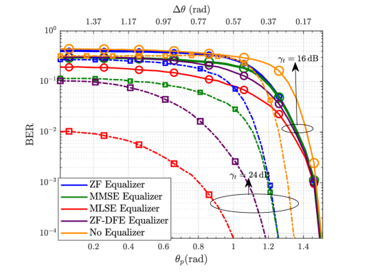
Figure 4: BER versus angles $\theta_{p}$ and $\Delta\theta$.

Fig. 4 shows the BER versus angles $\theta_{p}$ and $\Delta\theta=\frac{\pi}{2}-\theta_{p}$ for transmit SNRs $\gamma_{t}=16$ dB and 24 dB. To alleviate the ISI caused by delay spread, we employ maximum likelihood sequence estimation (MLSE), linear zero forcing (ZF) and minimum mean squared error (MMSE) equalization, and ZF-decision feedback equalization (ZF-DFE) at the Rx [25]. By increasing $\theta_{p}$ from 0 rad to $\pi\over 2$ rad (decreasing $\Delta\theta$), the number of dispersive FSO channel taps gradually decrease from 10 taps to 1 tap. Thus, we implemented MLSE using the Viterbi algorithm with $2^{9}$ states and linear equalizers with 20 taps. As can be observed, as $\theta_{p}$ increases, the BER decreases (even without equalizer) because of the smaller effective delay spread of the IRS-based FSO channel and the larger GML gain due to the higher received power at the lens. Our results also show that MLSE yields the best performance at the expense of higher complexity. Using linear equalization techniques, we can reduce the complexity compared to Viterbi algorithm. In particular, the MMSE equalizer performs better than the ZF equalizer for $\theta_{p}\leq 1.2$ rad ($\Delta\theta\geq 0.37$ rad), since the MMSE equalizer reduces noise enhancement. On the other hand, for $\theta_{p}>1.2$ rad ($\Delta\theta<0.37$ rad), the BER performance of the ZF equalizer matches that of the MMSE equalizer. Moreover, for $\gamma_{t}=16$ dB, both linear equalizers approach the performance of MLSE for $\theta_{p}>1.4$ rad ($\Delta\theta<0.17$ rad). Here, the difference between incident and reflected angles is very small, and as a result, the delay spread and ISI are also small. Moreover, ZF-DFE provides a good compromise between performance and complexity. It outperforms both linear equalizers but requires a much lower complexity compared to MLSE [25].

V Conclusions

In this paper, we investigated the delay dispersion introduced by an IRS in an FSO link. Using our analysis, we developed an analytical model for the delay profile and the continuous CIR of IRS-assisted FSO links. We showed that equalization techniques can be used to overcome the IRS-induced ISI. Our simulation results show that the positions of Tx and Rx w.r.t. the IRS, the IRS size, and the incident beamwidth affect the maximum delay spread and link performance. Moreover, using suitable equalization techniques the IRS-induced ISI can be resolved at the Rx.

Appendix A Proof of Theorem 1

Considering the received electric field in (14), and given $\tau(\mathbf{r})=\tau_{0}+a_{1}x+a_{2}y$, we obtain $\lVert\nabla{\tau}({\mathbf{r}})\rVert=\lVert[a_{1},a_{2}]^{T}\rVert=\sqrt{a_{1}^{2}+a_{2}^{2}}$. Then, using $\mathbf{r}(s)=[x(s),y(s)]^{T}=[s,\tilde{\tau}_{1}-\frac{a_{1}}{a_{2}}s]$, with $\tilde{\tau}_{1}=\frac{t-\tau_{0}}{a_{2}}$ and $-\frac{L_{x}}{2}\leq s\leq\frac{L_{x}}{2}$, we have $\lVert\nabla\mathbf{r}(s)\rVert=\lVert[1,-\frac{a_{1}}{a_{2}}]\rVert=\left[1+\left(\frac{a_{1}}{a_{2}}\right)^{2}\right]^{1\over 2}$. Thus, by substituting (9) and (4), we obtain

$$E_{\text{rx}}(\mathbf{r}_{o},t)=\frac{E_{0}w_{0}\zeta}{\mathrm{j}\lambda d_{p}|a_{2}|w(d_{l})}e^{-\mathrm{j}k(d_{l}+d_{p})+\mathrm{j}\psi_{0}-\mathrm{j}k\Phi_{0}}e^{-c_{2}\tilde{\tau}_{1}^{2}-c_{4}\tilde{\tau}_{1}}$$

$$\times\int_{-\frac{L_{x}}{2}}^{\frac{L_{x}}{2}}e^{-a_{s}s^{2}-b_{s}s}\mathrm{d}s$$

$$\overset{(i)}{=}\frac{E_{0}w_{0}\zeta}{2\lambda d_{p}|a_{2}|w(d_{l})}\sqrt{\frac{\pi}{a_{s}}}e^{-\mathrm{j}k(d_{l}+d_{p})+\mathrm{j}\psi_{0}}e^{-c_{2}\tilde{\tau}_{1}^{2}-c_{4}\tilde{\tau}_{1}}e^{\frac{b_{s}^{2}}{4a_{s}}}$$

$$\times\left[\text{erf}\left(\frac{\sqrt{a_{s}}L_{x}}{2}+\frac{b_{s}}{2\sqrt{a_{s}}}\right)-\text{erf}\left(-\frac{\sqrt{a_{s}}L_{x}}{2}+\frac{b_{s}}{2\sqrt{a_{s}}}\right)\right],\qquad$$ (19)

where in $(i)$ we use [26, (2.33-1)]. Moreover, $\bar{c}_{1}=\frac{1}{w_{x}^{2}(d_{l})}+\frac{\mathrm{j}k}{2d_{p}}\left(1-\frac{x_{o}^{2}}{d_{p}^{2}}\right)+\frac{\mathrm{j}k}{2R_{x}(d_{l})}$, $\bar{c}_{2}=\frac{1}{w_{y}^{2}(d_{l})}+\frac{\mathrm{j}k}{2d_{p}}\left(1-\frac{y_{o}^{2}}{d_{p}^{2}}\right)+\frac{\mathrm{j}k}{2R_{y}(d_{l})}$, $c_{3}=\frac{-\mathrm{j}kx_{o}}{d_{p}}+\mathrm{j}k\Phi_{x}-\mathrm{j}k\cos(\theta_{l})$, $c_{4}=\frac{-\mathrm{j}ky_{o}}{d_{p}}+\mathrm{j}k\Phi_{y}$, $\bar{c}_{5}=-\mathrm{j}k\frac{x_{o}y_{o}}{d_{p}^{3}}$, and $b_{s}=c_{3}-\frac{a_{1}}{a_{2}}c_{4}+\tilde{\tau}_{1}(c_{5}-2\frac{a_{1}}{a_{2}})c_{2}$.

Then, assuming $L_{x}\gg{2\over\sqrt{a_{s}}}$, we obtain the power density, defined as $I_{\text{rx}}(\mathbf{r}_{o},t)=\frac{1}{2\eta P_{0}}\left|E_{\text{rx}}(\mathbf{r}_{o},t)\right|^{2}$, as follows

$$I_{\text{rx}}(\mathbf{r}_{o},t) =C_{h}\exp\left(\frac{1}{2a_{s}}\left(c_{3}-c_{4}\frac{a_{1}}{a_{2}}\right)^{2}\right)$$ (20)

$$\times\exp\Biggl{(}-\tilde{\tau}_{1}^{2}\left(2c_{2}-\left(c_{5}-2\frac{a_{1}}{a_{2}}\right)^{2}\frac{c_{2}^{2}}{2a_{s}}\right)$$

$$-\tilde{\tau}_{1}\left(2c_{4}-\frac{c_{2}}{a_{s}}\left(c_{5}-2\frac{a_{1}}{a_{2}}\right)\left(c_{3}-\frac{a_{1}}{a_{2}}c_{4}\right)\right)\Biggl{)}.\qquad$$

Then, we apply $\mathbf{r}_{o}=\mathbf{R}_{3}\left[\mathbf{r}_{p}^{T},d_{p}\right]^{T}$ and approximate $\frac{x_{o}^{2}}{d_{p}^{2}}\approx\cos^{2}(\phi_{p})\cos^{2}(\theta_{p})$, $\frac{y_{o}^{2}}{d_{p}^{2}}\approx\sin^{2}(\phi_{p})\cos^{2}(\theta_{p})$, and $\frac{x_{o}y_{o}}{d_{p}^{2}}\approx\sin(\phi_{p})\cos(\phi_{p})\cos^{2}(\theta_{p})$ [5], which leads to $\bar{c}_{1}\approx c_{1}$, $\bar{c}_{2}\approx c_{2}$, and $\bar{c}_{5}\approx c_{5}$. Then, by applying the values of $\Phi_{x}$ and $\Phi_{y}$ in (4) and substituting $[c_{3},c_{4}]^{T}=\mathbf{D}\mathbf{r}_{p}$ and (20) in (7), we obtain (15). This completes the proof.

Appendix B Proof of Corollary 1

Given (14) and $\tau(\mathbf{r})=a_{1}x+\tau_{0}$, we can substitute $\mathbf{r}(s)=[\tilde{\tau}_{2},s]^{T}$ with $\tilde{\tau}_{2}=\frac{t-\tau_{0}}{a_{1}}$ and $-\frac{L_{y}}{2}\leq s\leq\frac{L_{y}}{2}$. Using similar approximations as in the proof of Theorem 1, the received electric field at the lens obtained as

$$E_{\text{rx}}(\mathbf{r}_{o},t)=\frac{1}{|a_{1}|}\int_{-\frac{L_{y}}{2}}^{\frac{L_{y}}{2}}E(\mathbf{r}(s))e^{-\mathrm{j}\phi(\mathbf{r}(s),\mathbf{r}_{o})}\mathrm{d}s$$

$$=C_{e}e^{-\mathrm{j}k\phi_{e}+\mathrm{j}\psi_{0}}\exp\left(-\frac{(\tilde{\tau}_{2})^{2}}{w_{x}^{2}(d_{l})}\right)\int_{-\frac{L_{y}}{2}}^{\frac{L_{y}}{2}}e^{-b_{y}s^{2}-y(\mathrm{j}k\frac{y_{p}}{d_{p}})}\mathrm{d}s$$

$$=C_{e}e^{-\mathrm{j}k\phi_{e}+\mathrm{j}\psi_{0}}\frac{\sqrt{\pi}}{2\sqrt{b_{y}}}\exp\left(-\frac{(\tilde{\tau}_{2})^{2}}{w_{x}^{2}(d_{l})}\right)\exp\left(\frac{-k^{2}y_{p}^{2}}{4b_{y}d_{p}^{2}}\right)\times$$

$$\left[\text{erf}\left(\!\!\sqrt{b_{y}}\frac{L_{y}}{2}+\frac{\mathrm{j}ky_{p}}{2d_{p}\sqrt{b_{y}}}\!\right)-\text{erf}\left(\!\!-\sqrt{b_{y}}\frac{L_{y}}{2}+\frac{\mathrm{j}ky_{p}}{2d_{p}\sqrt{b_{y}}}\!\right)\!\right]\!,\quad$$ (21)

where $C_{e}=\frac{v_{l}\zeta E_{0}w_{0}}{\lambda d_{p}|a|w(d_{l})}$, $\phi_{e}=d_{l}+d_{p}-\tilde{\tau}(\cos(\theta_{l})-\cos(\theta_{p}))+\frac{(\tilde{\tau}_{2})^{2}}{2R_{x}(d_{l})}-{\tilde{\tau}_{2}}\frac{\sin(\theta_{p})x_{p}}{d_{p}}+\left(\tilde{\tau}_{2}\right)^{2}\frac{\sin^{2}(\theta_{p})}{2d_{p}}+\Phi_{x}\tilde{\tau}_{2}$.

Assuming $L_{y}\gg\frac{2}{\sqrt{b_{y}}}$, we can simplify the received beam intensity as follows

$$I_{\text{rx}}(\tau,\mathbf{r}_{p})=\frac{C_{e}^{2}\pi}{2\eta P_{0}|b_{y}|}e^{-2\frac{\tilde{\tau}_{2}^{2}}{w_{x}^{2}(d_{l})}}\exp\left(\frac{-k^{2}y_{p}^{2}\mathcal{R}\{b_{y}\}}{2|b_{y}|^{2}d_{p}^{2}}\right),\qquad$$ (22)

where $\mathcal{R}\{\cdot\}$ denotes the real part of a complex number. Next, we obtain the GML factor in (7) as follows

$$h_{\text{gml}}(\tau) =\frac{C_{e}^{2}\pi}{2\eta P_{0}|b_{y}|}e^{-\frac{2(\tilde{\tau}_{2})^{2}}{w_{x}^{2}(d_{l})}}\iint_{\Sigma_{\text{lens}}}\exp\left(\frac{-k^{2}y_{p}^{2}\mathcal{R}\{b_{y}\}}{2|b_{y}|^{2}d_{p}^{2}}\right)\mathrm{d}x_{p}\mathrm{d}y_{p}$$ (23)

$$\overset{(i)}{=}C_{h}\exp\left(-\frac{2\tilde{\tau}_{2}^{2}}{w_{x}^{2}(d_{l})}\right)\text{erf}\left(\frac{k\tilde{a}}{\sqrt{2}w(d_{l})|b_{y}|d_{p}}\right),$$

where in $(i)$, we use $\int e^{ax^{2}}\mathrm{d}x=\frac{1}{2}\sqrt{\frac{\pi}{a}}\text{erfi}(\sqrt{a}x)$ and $\text{erfi}(x)=-\mathrm{j}\text{erf}(\mathrm{j}x)$. Moreover, $C_{h}=\sqrt{\frac{2}{\pi}}\frac{\zeta^{2}}{\lambda d_{p}|a_{1}|^{2}w(d_{l})}$. Substituting $\zeta$ from (18), we obtain (16) and this completes the proof.

Appendix C Proof of Proposition 1

Ignoring the impact of atmospheric loss and atmospheric turbulence and given the passivity of the IRS, the average received power over the dispersive channel should be equal to average transmitted power without delay given by

$$\bar{P}_{\text{rx}} =\int_{-\infty}^{\infty}P_{0}h_{\text{gml}}(t)\mathrm{d}t$$ (24)

$$=P_{0}C_{h}\text{erf}\left(\frac{k\tilde{a}}{\sqrt{2}w(d_{l})|b_{y}|d_{p}}\right)\int_{-\infty}^{\infty}\exp\left(-\frac{2(\tilde{\tau}_{2})^{2}}{w_{x}^{2}(d_{l})}\right)\mathrm{d}t$$

$$\overset{(i)}{=}P_{0}\frac{\zeta^{2}}{\lambda d_{p}|a_{1}|\sin(\theta_{l})}\text{erf}\left(\frac{k\tilde{a}}{\sqrt{2}w(d_{l})|b_{y}|d_{p}}\right),$$

where in $(i)$ we use $\int_{-\infty}^{\infty}\exp(-p^{2}x^{2}-qx)\,\mathrm{d}x=\frac{\sqrt{\pi}}{p}\exp\left(\frac{q^{2}}{4p^{2}}\right)$ [26, (3.323-2)]. Comparing (24) with average transmit power $P_{0}$ leads to (18) and completes the proof.

References

• [1] W. Saad, M. Bennis, and M. Chen, “A vision of 6G wireless systems: Applications, trends, technologies, and open research problems,” IEEE Network, vol. 34, no. 3, pp. 134–142, May/June 2020.
• [2] H. Ajam, M. Najafi, V. Jamali, and R. Schober, “Power scaling law for optical IRSs and comparison with optical relays,” in Proc. IEEE Globecom, 2022, pp. 1527–1533.
• [3] V. Jamali, H. Ajam, M. Najafi, B. Schmauss, R. Schober, and H. V. Poor, “Intelligent reflecting surface assisted free-space optical communications,” IEEE Commun. Mag., vol. 59, no. 10, pp. 57–63, 2021.
• [4] M. Najafi and R. Schober, “Intelligent reflecting surfaces for free space optical communications,” in Proc. IEEE Globecom, 2019, pp. 1–7.
• [5] H. Ajam, M. Najafi, V. Jamali, B. Schmauss, and R. Schober, “Modeling and design of IRS-assisted multi-link FSO systems,” IEEE Trans. Commun., vol. 70, no. 5, pp. 3333–3349, 2022.
• [6] M. Najafi, B. Schmauss, and R. Schober, “Intelligent reflecting surfaces for free space optical communication systems,” IEEE Trans. Commun., vol. 69, no. 9, pp. 6134–6151, 2021.
• [7] A. R. Ndjiongue, T. M. N. Ngatched, O. A. Dobre, A. G. Armada, and H. Haas, “Analysis of RIS-based terrestrial-FSO link over G-G turbulence with distance and jitter ratios,” J. Lightwave Technology, vol. 39, no. 21, pp. 6746–6758, 2021.
• [8] H. Ajam, M. Najafi, V. Jamali, and R. Schober, “Channel modeling for IRS-assisted FSO systems,” in Proc. IEEE WCNC, 2021, pp. 1–7.
• [9] ——, “Optical irss: Power scaling law, optimal deployment, and comparison with relays,” IEEE Trans. Commun., 2023.
• [10] M. Najafi, V. Jamali, R. Schober, and H. V. Poor, “Physics-based modeling and scalable optimization of large intelligent reflecting surfaces,” IEEE Trans. Commun., vol. 69, no. 4, pp. 2673–2691, 2021.
• [11] A. R. Ndjiongue, T. M. N. Ngatched, O. A. Dobre, and H. Haas, “Design of a power amplifying-RIS for free-space optical communication systems,” IEEE Wireless Commun., vol. 28, no. 6, pp. 152–159, 2021.
• [12] Z. Zhang, Y. Yin, and G. M. Rebeiz, “Intersymbol interference and equalization for large 5G phased arrays with wide scan angles,” IEEE Trans. Microw. Theory Tech., vol. 69, no. 3, pp. 1955–1964, 2021.
• [13] C. Chen, S. Huang, H. Abumarshoud, I. Tavakkolnia, M. Safari, and H. Haas, “Frequency-domain channel characteristics of intelligent reflecting surface assisted visible light communication,” J. Lightwave Technology, vol. 41, no. 24, pp. 7355–7369, 2023.
• [14] S. Hranilovic, “Minimum-bandwidth optical intensity Nyquist pulses,” IEEE Trans. Commun., vol. 55, no. 3, pp. 574–583, 2007.
• [15] D. Plabst, F. J. G. Gómez, T. Wiegart, and N. Hanik, “Wiener filter for short-reach fiber-optic links,” IEEE Commun. Lett., vol. 24, no. 11, pp. 2546–2550, 2020.
• [16] J. Kahn, W. Krause, and J. Carruthers, “Experimental characterization of non-directed indoor infrared channels,” IEEE Trans. Commun., vol. 43, no. 2/3/4, pp. 1613–1623, 1995.
• [17] J. Kahn and J. Barry, “Wireless infrared communications,” Proc. IEEE, vol. 85, no. 2, pp. 265–298, 1997.
• [18] M. Grabner and V. Kvicera, “Multiple scattering in rain and fog on free-space optical links,” J. Lightwave Technology, vol. 32, no. 3, pp. 513–520, 2014.
• [19] M. A. Khalighi and M. Uysal, “Survey on free space optical communication: A communication theory perspective,” IEEE Commun. Surveys Tuts., vol. 16, Fourthquarter 2014.
• [20] J. W. Goodman, Introduction to Fourier Optics.   Roberts & Co., 2005.
• [21] L. C. Andrews and R. L. Phillips, Laser Beam Propagation through Random Media.   Bellingham, Washington: SPIE Press, 2005.
• [22] A. Goldsmith, Wireless Communications.   Cambridge Univ. Press, 2005.
• [23] L. W. Barclay, Propagation of Radiowaves.   Institution of Engineering and Technology (IET), 2003.
• [24] L. Zhang, “Dirac delta function of matrix argument,” International Journal of Theoretical Physics, vol. 60, p. 2445–2472, 2021.
• [25] J. G. Proakis and M. Salehi, Digital Communications.   McGraw Hill, 2007.
• [26] I. S. Gradshteyn and I. M. Ryzhik, Table of Integrals, Series, and Products.   San Diego, CA: Academic, 1994.