Intelligent Reflecting Surfaces vs. Full-Duplex Relays: A Comparison in the Air

Abstract

This letter aims to provide a fundamental analytical comparison for the two major types of relaying methods: intelligent reflecting surfaces and full-duplex relays, particularly focusing on unmanned aerial vehicle communication scenarios. Both amplify-and-forward and decode-and-forward relaying schemes are included in the comparison. In addition, optimal 3D UAV deployment and minimum transmit power under the quality of service constraint are derived. Our numerical results show that IRSs of medium size exhibit comparable performance to AF relays, meanwhile outperforming DF relays under extremely large surface size and high data rates.

I Introduction

Intelligent reflecting surface (IRS) is a revolutionizing architecture that can modify the amplitude and phase of incident signals via controllable reflection, to enhance the performance of wireless communication networks[1]. As a complementary device, IRS could be easily installed on the walls, ceilings and facades of buildings, benefiting from its low fabrication costs and light weight[2]. Although the ease of deployment is quite appealing, some fundamental limitations remain. First, deploying an IRS at a fixed place potentially reduces its coverage since it only serves a limited and fixed area. Second, line-of-sight (LoS) paths are typically difficult to maintain due to complex environments near ground. As a result, the signals will be severely attenuated after undergoing several reflections. Third, it is practically difficult to deploy IRSs considering environmental and civil constraints. To unlock the limitations of terrestrial IRSs, it is promising to deploy an IRS on an unmanned aerial vehicle (UAV), known as UAV-IRS, aerial IRS or UAV-mounted/borne/carried IRS[3]. Thanks to its mobility, UAV-IRS could bypass the obstacles to establish LoS links with ground users. More significantly, wider coverage range is realized through full-angle reflection towards the ground.

Despite the attractiveness of UAV-IRS, it is strongly encouraged to compare this integration with traditional full-duplex UAV-relay, given that previous literature mainly focused on the comparison in terrestrial scenarios[1, 4, 5, 6, 7, 8, 9, 10]. In [11], the authors reviewed the differences and similarities between full-duplex relays and IRSs. In [1] and [4], the authors showed that IRSs could achieve 300% higher energy efficiency against half-duplex amplify-and-forward (AF) relays while the authors of [5] pointed out that IRSs could outperform half-duplex decode-and-forward (DF) relays only under large surfaces and/or high data rates. Furthermore, AF full-duplex relays and IRSs were compared in MIMO systems by optimizing the beamforming matrices[6, 7]. Differently, [8] showed that IRSs could outperform DF full-duplex relays in terms of outage probability and energy efficiency. More recently, [9] presented that IRSs had a huge performance loss compared to DF full-duplex relays. In[10], IRSs were compared with AF and DF relays, however, only some experimental results were provided, with no further theoretical analysis. In a nutshell, fair comparison between IRSs and relays including both AF and DF protocols, as well as mathematical analysis are needed and yet not provided.

Since IRSs could be interpreted as full-duplex[2], we thus perceive full-duplex relays as fairer comparison targets. Our goal is to provide a fundamental analytical comparison between IRSs and full-duplex relays including AF and DF schemes, specifically in UAV communication networks. For fairness of comparison, we prove the optimal 3D deployment of UAV and derive the minimum transmit power under quality of service (QoS) constraint for IRS, AF and DF relays. The novel contribution will underpin the emerging paradigm of integrated perception, communication and control (IPCC) design. Further, numerical simulations are conducted to effectively compare IRSs against full-duplex relays and justify the proposed theorems.

II System Model

To study the fundamental performance for fair comparison between the two types of relaying technologies, we consider a classic three-node system model comprised of a single-antenna source (S), a single-antenna destination (D) and an aerial node (R), i.e., UAV-IRS or UAV-relay, as shown in Fig. 1. The IRS is installed with $N=N_{x}N_{y}$ elements while the full-duplex relay is equipped with two uniform planar arrays (UPAs) of size $N$ separately used for transmission and reception. It is assumed that the direct link between S and D suffers from deep fading and thus is negligible[5, 9]. The UAV helps establish LoS transmission links with S and D in order to relay signals. The coordinates of S, D and R are given by $(0,0,0)$, $(L,0,0)$ and $(x_{U},y_{U},h_{U})$, respectively. Hence the deterministic air-to-ground channel gain from S to R and that from R to D are, respectively, expressed by[12, 13]

$$g_{SR}=\beta_{0}d_{SR}^{-2},\quad g_{RD}=\beta_{0}d_{RD}^{-2},$$ (1)

with $\beta_{0}$ denoting the channel gain at a reference distance of 1m, $d_{SR}=\sqrt{x_{U}^{2}+y_{U}^{2}+h_{U}^{2}}$ and $d_{RD}=\sqrt{(x_{U}-L)^{2}+y_{U}^{2}+h_{U}^{2}}$. Further, the channel vectors from S to R and that from R to D are given by, respectively,

$$\mathbf{h}_{SR}=\sqrt{g_{SR}}\mathbf{a}_{SR},\quad\mathbf{h}_{RD}=\sqrt{g_{RD}}\mathbf{a}_{RD},$$ (2)

with $\mathbf{a}_{i}=[1,\ldots,e^{-j\frac{2\pi}{\lambda}d\sin\theta_{i}[(n_{x}-1)\cos\phi_{i}+(n_{y}-1)\sin\phi_{i}]},\ldots,$ $e^{-j\frac{2\pi}{\lambda}d\sin\theta_{i}[(N_{x}-1)\cos\phi_{i}+(N_{y}-1)\sin\phi_{i}]}]^{T},i\in\{SR,RD\}$. $\lambda$ represents the wavelength and $d$ denotes antenna separation. $n_{x}$ and $n_{y}$ denote the indexes of antenna along horizontal and vertical directions, respectively. $\theta_{i}$ and $\phi_{i}$ denote the corresponding elevation and azimuth angles, respectively.

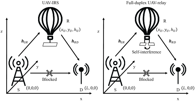
Figure 1: Illustration of three-node systems

II-A IRS-assisted networks

In this setup, we let diagonal matrix $\mathbf{\Psi}=\text{diag}(e^{j\psi_{1}},\ldots,e^{j\psi_{N}})$ represent the passive beamforming of IRS, and thus the received signal at D is denoted by $y_{D}^{(IRS)}=\mathbf{h}_{RD}^{H}\mathbf{\Psi}\mathbf{h}_{SR}\sqrt{p_{S}^{(IRS)}}s+n_{D}$, where $p_{S}^{(IRS)}$ denotes the transmit power of S, $s$ represents the transmit signal with unit power and $n_{D}\sim\mathcal{CN}(0,\sigma^{2})$ is the noise at D. Thereby, the corresponding capacity is

$$R_{IRS} =\log_{2}\bigg{(}1+\frac{p_{S}^{(IRS)}|\mathbf{h}_{RD}^{H}\mathbf{\Psi}\mathbf{h}_{SR}|^{2}}{\sigma^{2}}\bigg{)}$$ (3)

$$\overset{(a)}{=}\log_{2}\bigg{(}1+\frac{N^{2}p_{S}^{(IRS)}g_{SR}g_{RD}}{\sigma^{2}}\bigg{)},$$

where $(a)$ holds by adopting coherent phase shifting scheme $\psi_{n}=j\frac{2\pi}{\lambda}d\{\sin\theta_{SR}[(n_{x}-1)\cos\phi_{SR}+(n_{y}-1)\sin\phi_{SR}]-\sin\theta_{RD}[(n_{x}-1)\cos\phi_{RD}+(n_{y}-1)\sin\phi_{RD}]\},\forall n=n_{x}n_{y}$[5]. The beam alignment for the high-mobility UAV-IRS can be achieved using the framework in [14]. As expected, the received power increases in the order of $\mathcal{O}(N^{2})$[2].

II-B AF full-duplex relay-assisted networks

In this case, the full-duplex relay simultaneously receives and transmits signals with AF scheme. Hence, the received signal at relay is given by $\mathbf{y}_{R}^{(AF)}=\sqrt{p_{S}^{(AF)}}\mathbf{h}_{SR}s+\sqrt{\rho p_{R}^{(AF)}}\mathbf{\tilde{y}}_{R}^{(AF)}+\mathbf{n}_{R}$, where $p_{S}^{(AF)}$ and $p_{R}^{(AF)}$ denote the transmit power of S and AF relay, respectively. $\rho$ characterizes the effects of self-interference cancellation, $\mathbf{n}_{R}\sim\mathcal{CN}(0,\sigma^{2}\mathbf{I}_{N})$ is the noise, and $\mathbf{\tilde{y}}_{R}^{(AF)}$ is a delayed and distorted replica of $\mathbf{y}_{R}^{(AF)}$. Without loss of generality, we assume $\mathbf{\tilde{y}}_{R}^{(AF)}\sim\mathcal{CN}(0,\mathbf{I}_{N})$[15]. Then the received signal is processed with combiner $\mathbf{v}$ and forward with precoder $\mathbf{w}$, where $\|\mathbf{v}\|=1$ and $\|\mathbf{w}\|=1$. Therefore, the received signal at D is expressed by

$$y_{D}^{(AF)} \!=\!\sqrt{p_{R}^{(AF)}}\mathbf{h}_{RD}^{H}\mathbf{w}\mathbf{v}^{H}\mathbf{y}_{R}^{(AF)}+n_{D}$$ (4)

$$\!=\!\sqrt{\!p_{R}^{(AF)}p_{S}^{(AF)}}\mathbf{h}_{RD}^{H}\mathbf{w}\mathbf{v}^{H}\mathbf{h}_{SR}s$$

$$\!+\!\sqrt{\!\rho}p_{R}^{(AF)}\mathbf{h}_{RD}^{H}\mathbf{w}\mathbf{v}^{H}\tilde{\mathbf{y}}_{R}^{(AF)}\!\!+\!\!\sqrt{\!p_{R}^{(AF)}}\mathbf{h}_{RD}^{H}\mathbf{w}\mathbf{v}^{H}\mathbf{n}_{R}\!+\!n_{D}.$$

$$R_{AF} =\!\mathbb{E}\left[\log_{2}\left(1+\frac{p_{R}^{(AF)}p_{S}^{(AF)}|\mathbf{h}_{RD}^{H}\mathbf{w}\mathbf{v}^{H}\mathbf{h}_{SR}|^{2}}{\rho(p_{R}^{(AF)})^{2}|\mathbf{h}_{RD}^{H}\mathbf{w}\mathbf{v}^{H}\tilde{\mathbf{y}}_{R}^{(AF)}|^{2}+p_{R}^{(AF)}|\mathbf{h}_{RD}^{H}\mathbf{w}\mathbf{v}^{H}\mathbf{n}_{R}|^{2}+|n_{D}|^{2}}\right)\right]$$ (5)

$$\overset{(b)}{\leq}\!\log_{2}\!\left(\!1\!+\!\frac{p_{R}^{(AF)}p_{S}^{(AF)}\mathbb{E}\left[|\mathbf{h}_{RD}^{H}\mathbf{w}\mathbf{v}^{H}\mathbf{h}_{SR}|^{2}\right]}{(N\rho(p_{R}^{(AF)})^{2}+N\sigma^{2}p_{R}^{(AF)})\mathbb{E}[|\mathbf{h}_{RD}^{H}\mathbf{w}|^{2}]+\sigma^{2}}\!\right)\overset{(c)}{=}\log_{2}\!\left(\!1\!+\!\frac{N^{2}p_{R}^{(AF)}p_{S}^{(AF)}g_{SR}g_{RD}}{(N\rho(p_{R}^{(AF)})^{2}+N\sigma^{2}p_{R}^{(AF)})g_{RD}+\sigma^{2}}\!\right).$$

 

The achievable rate of AF relay-aided networks is derived as (5) at the top of next page, where $(b)$ holds due to Jensen’s inequality and the fact that $\mathbb{E}[\|\tilde{\mathbf{y}}_{R}^{(AF)}\|^{2}]=N,\mathbb{E}[\|\mathbf{n}_{R}\|]=\sigma^{2}N,\mathbb{E}[|n_{R}|^{2}]=\sigma^{2},\|\mathbf{w}\|^{2}=1$ and $\|\mathbf{v}\|^{2}=1$; $(c)$ holds by using maximum ratio transmission and combing scheme $\mathbf{v}=\frac{\mathbf{h}_{SR}}{\|\mathbf{h}_{SR}\|}$, $\mathbf{w}=\frac{\mathbf{h}_{RD}}{\|\mathbf{h}_{RD}\|}$[6] and the fact that $\mathbb{E}[\|\mathbf{h}_{SR}\|^{2}]=Ng_{SR}$ and $\mathbb{E}[\|\mathbf{h}_{RD}\|^{2}]=Ng_{RD}$.

II-C DF full-duplex relay-assisted networks

With DF relaying protocol, the relay first decodes the received signal, which is given by $\mathbf{y}_{R}^{(DF)}=\sqrt{p_{S}^{(DF)}}\mathbf{h}_{SR}s+\sqrt{\rho p_{R}^{(DF)}}\tilde{\mathbf{s}}+\mathbf{n}_{R}$, where $p_{S}^{(DF)}$ and $p_{R}^{(DF)}$ denote the transmit power of S and DF relay, respectively. $\tilde{\mathbf{s}}\sim\mathcal{CN}(0,\mathbf{I}_{N})$ is a delayed and distorted replica of $\mathbf{w}s$. After decoding the information, DF relay encodes it for further transmission and the signal received by D is $y_{D}^{(DF)}=\sqrt{p_{R}^{(DF)}}\mathbf{h}^{H}_{RD}\mathbf{w}s+n_{D}$. Following the similar analysis to (5), the achievable rate of DF relay-aided networks is

$$\color[rgb]{0,0,1}R_{DF}\leq\log_{2}\bigg{(}1+\min\bigg{(}\frac{p_{S}^{(DF)}g_{SR}}{\rho p_{R}^{(DF)}+\sigma^{2}},\frac{Np_{R}^{(DF)}g_{RD}}{\sigma^{2}}\bigg{)}\bigg{)}.$$ (6)

III 3D UAV deployment optimization

In this section, we provide rigorous proof for optimal UAV deployment. It is assumed that UAV could move horizontally in a wide area $\mathcal{A}$ covering S and D while it could fly vertically at the altitude ranging from $h_{min}$ to $h_{max}$, where $h_{min}$ denotes the minimum height to maintain an LoS path, and $h_{max}$ means the maximum tolerable height.

III-A IRS-assisted networks

Here we start with IRS to draw some useful insights. Considering the deployment constraints and substituting (1) into (3), we can express the UAV positioning problem as

$$\max_{x_{U},y_{U},h_{U}} R_{IRS}=\log_{2}\bigg{(}1+\frac{N^{2}p_{S}^{(IRS)}\beta_{0}^{2}}{\sigma^{2}d_{SR}^{2}d_{RD}^{2}}\bigg{)}$$ (7a)

s.t. $$(x_{U},y_{U})\in\mathcal{A},h_{min}\leq h_{U}\leq h_{max}.$$ (7b)

We observe that only the denominator in (7a) is related to the UAV position. Thus problem (7) is reduced to

$$\min_{x_{U},y_{U},h_{U}} f(x_{U},y_{U},h_{U})=d_{SR}^{2}d_{RD}^{2}$$

$$=(x_{U}^{2}+y_{U}^{2}+h_{U}^{2})\big{(}(x_{U}-L)^{2}+y_{U}^{2}+h_{U}^{2}\big{)}$$ (8a)

s.t. $$\eqref{cons:UAV deployment for IRS}.$$ (8b)

Lemma 1.

The optimal solution to problem (8) is

$$x_{U}^{*}=\left\{\begin{aligned} &\frac{L}{2},\quad\text{if}\ \ L\leq 2h_{min}\\ &\frac{L}{2}\pm\sqrt{\frac{L^{2}}{4}-h_{min}^{2}},\quad\text{if}\ \ L>2h_{min}\end{aligned}\right.,$$ (9)

$$y_{U}^{*}=0,h_{U}^{*}=h_{min}.$$ (10)

Proof.

See Appendix A. ∎

Remark 1.

Lemma 1 states that UAV should hover at the midpoint of S and D if its flight altitude is relatively high. Otherwise, the UAV should hover near to either S or D when its flight altitude is relatively low.

III-B AF full-duplex relay-assisted networks

For AF relays, we substitute (1) into (5) and follow the steps in the IRS case. A simplified UAV deployment problem is expressed by

$$\min_{x_{U}}\quad\xi_{1}\tilde{g}(x_{U})+\xi_{2}\tilde{f}(x_{U}),\quad\text{s.t.}\quad x_{U}\in[0,L],$$ (11)

where $\xi_{1}=\frac{\rho p_{R}^{(AF)}+\sigma^{2}}{N\beta_{0}p_{S}^{(AF)}}$, $\xi_{2}=\frac{\sigma^{2}}{N^{2}\beta_{0}^{2}p_{S}^{(AF)}p_{R}^{(AF)}}$, $\tilde{g}(x_{U})=x_{U}^{2}+h_{min}^{2}$ and $\tilde{f}(x_{U})$ is defined in Lemma 1.

Lemma 2.

The optimal solution to problem (11) satisfies $\tilde{x}^{*}_{U}\in[0,x_{U}^{*}]$, with $x_{U}^{*}$ being defined in Lemma 1.

Proof.

First, the solution to minimize $\xi_{2}\tilde{f}(x_{U})$ is defined in Lemma 1. Further, we could see that $\tilde{g}(x_{U})$ is increasing over $x_{U}\in[0,L]$, and as a result the optimal solution of $\xi_{1}\tilde{g}(x_{U})+\xi_{2}\tilde{f}(x_{U})$ is no greater than that of sole $\xi_{2}\tilde{f}(x_{U})$, which proves Lemma 2. ∎

Although we have Lemma 2, it is still non-trivial to write the expression of optimal solution. Fortunately, it could be readily proved that $\tilde{f}(x_{U})$ and $\tilde{g}(x_{U})$ are convex over the intervals of interest, and thus $\xi_{1}\tilde{g}(x_{U})+\xi_{2}\tilde{f}(x_{U})$ is also convex. Therefore, one-dimensional searching methods such as golden section search can be adopted to obtain the optimal solution efficiently.

Remark 2.

Lemma 2 reveals that the UAV should never be placed at D side in the AF relay case. Moreover, if we define $\xi\triangleq\frac{\xi_{1}}{\xi_{2}}=\frac{N\beta_{0}p_{R}^{(AF)}(\rho p_{R}^{(AF)}+\sigma^{2})}{\sigma^{2}}$, we could intuitively deduce that the UAV deployment only depends on $p_{R}^{(AF)}$, $N$, $L$ and $h_{min}$. If $p_{R}^{(AF)}\rightarrow+\infty$, then $\xi\gg 1$ and $\tilde{g}(x_{U})$ becomes dominant. To minimize $\tilde{g}(x_{U})$, we have $\tilde{x}_{U}^{*}\rightarrow 0$. On the other hand, if $p_{R}^{(AF)}\rightarrow 0$, then $\xi\ll 1$ and $\tilde{f}(x_{U})$ becomes dominant. In this case, $\tilde{x}_{U}^{*}$ will be close to Lemma 1.

III-C DF full-duplex relay-assisted networks

For ease of notation, we denote $\mu_{1}=\frac{p_{S}^{(DF)}}{\rho p_{R}^{(DF)}+\sigma^{2}}$ and $\mu_{2}=\frac{Np_{R}^{(DF)}}{\sigma^{2}}$. Our goal is to maximize the minimum value between $\mu_{1}g_{SR}$ and $\mu_{1}g_{RD}$. Note that in the DF case, we similarly have $y_{U}^{*}=0$ and $h_{U}^{*}=h_{min}$, which leads to a much simpler problem as follows,

$$\max_{x_{U}}\min\left\{\frac{\mu_{1}}{\tilde{g}(x_{U})},\frac{\tilde{g}(x_{U})\mu_{2}}{\tilde{f}(x_{U})}\right\}\quad\text{s.t.}\ x_{U}\in[0,L],$$ (12)

with $\tilde{g}(x_{U})$ and $\tilde{f}(x_{U})$ being defined in problem (11).

Lemma 3.

The optimal solution to problem (12) is

$$x_{U}^{*}=\left\{\begin{aligned} &0,\quad\text{if}\ \ \mu_{1}\leq\nu\mu_{2}\\ &L,\quad\text{if}\ \ \mu_{1}\geq\frac{1}{\nu}\mu_{2}\\ &\frac{L}{2},\quad\text{if}\ \ \mu_{1}=\mu_{2}\\ &kL\!+\!\sqrt{k^{2}L^{2}\!-kL^{2}\!-h_{min}^{2}},\ \text{if}\ \ \nu\mu_{2}<\mu_{1}<\mu_{2}\\ &kL\!-\!\sqrt{k^{2}L^{2}\!-kL^{2}\!-h_{min}^{2}},\ \text{if}\ \ \mu_{2}<\mu_{1}<\frac{1}{\nu}\mu_{2}\end{aligned}\right.,$$ (13)

with $\nu=\frac{h_{min}^{2}}{L^{2}+h_{min}^{2}}$ and $k=\frac{\mu_{1}}{\mu_{1}-\mu_{2}}$.

Proof.

First, it can be seen that $\frac{\mu_{1}}{\tilde{g}(x_{U})}$ is always no greater than $\frac{\tilde{g}(x_{U})\mu_{2}}{\tilde{f}(x_{U})}$ if $\mu_{1}\leq\nu\mu_{2}$. To maximize $\frac{\mu_{1}}{\tilde{g}(x_{U})}$, we shall have $x_{U}^{*}=0$. Similarly, we need to maximize $\frac{\tilde{g}(x_{U})\mu_{2}}{\tilde{f}(x_{U})}$ when $\mu_{1}\geq\frac{1}{\nu}\mu_{2}$, which yields $x_{U}^{*}=L$. When $\nu\mu_{2}<\mu_{1}<\frac{1}{\nu}\mu_{2}$, the optimal solution is obtained by solving equation $\frac{\mu_{1}}{\tilde{g}(x_{U})}=\frac{\tilde{g}(x_{U})\mu_{2}}{\tilde{f}(x_{U})}$. If $\mu_{1}=\mu_{2}$, it is a linear equation with solution $x_{U}^{*}=\frac{L}{2}$. Otherwise, it is a quadratic equation with its solutions defined in Lemma 3. ∎

Remark 3.

Lemma 3 indicates that UAV deployment in the DF case depends on $p_{S}^{(DF)}$, $p_{R}^{(DF)}$, $N$, $L$ and $h_{min}$. If $\mu_{1}>\mu_{2}$, the UAV needs to be deployed at D side. Differently, under conditions $\mu_{1}<\mu_{2}$, the UAV ought to be placed near S.

IV Transmit power minimization under QoS constraint

Considering low energy consumption, the transmit power ought to be minimized, without violating the QoS requirement, say $R_{i}\geq R_{0},i\in\{IRS,AF,DF\}$. From (3), (5) and (6), it can be seen that data rates are non-decreasing with respect to transmit power. Therefore, the equality must hold at the optimal point and our goal transforms into finding the minimum transmit power under $R_{i}=R_{0},i\in\{IRS,AF,DF\}$, which is concluded in Proposition 1.

Proposition 1.

To achieve a data rate $R_{0}$, the minimum transmit power for IRS-aided networks scales down with $N^{2}$, denoted by

$$p_{S}^{(IRS)}=\frac{\sigma^{2}(2^{R_{0}}-1)}{N^{2}g_{SR}g_{RD}}.$$ (14)

The AF relay case requires the transmit power

$$p_{S}^{(\!AF\!)}\!\!+\!p_{R}^{(\!AF\!)}\!=\!2\sqrt{\!\frac{\sigma^{2}\!(\rho(2^{\!R_{0}}\!-1)\!+\!g_{SR})\!(2^{\!R_{0}}\!-\!1)}{N^{2}g_{SR}^{2}g_{RD}}}\!+\!\frac{\sigma^{2}(2^{\!R_{0}}\!-\!1)}{g_{SR}}.$$ (15)

The DF relay case requires the transmit power

$$\color[rgb]{0,0,1}p_{S}^{(DF)}\!+\!p_{R}^{(DF)}\!=\!\frac{\sigma^{2}\rho(2^{R_{0}}\!-\!1)^{2}}{Ng_{SR}g_{RD}}\!+\!\frac{\sigma^{2}(2^{R_{0}}\!-\!1)}{g_{SR}}\!+\!\frac{\sigma^{2}(2^{R_{0}}\!-\!1)}{Ng_{RD}}.$$ (16)

Proof.

See Appendix B. ∎

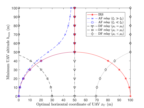
Figure 2: Optimal UAV deployment for IRS, AF and DF relays under $N=10$ and $L=100$m

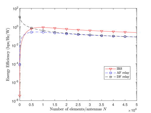
Figure 3: Energy efficiency versus $N$ under $L=200$m and $R_{0}=4$bps/Hz/W

V Numerical Results

In this section, we present numerical results to gain useful insights. We adopt an alternating optimization method[1] to handle the coupled nature of UAV deployment and transmit power. This approach involves iteratively updating each variable while keeping the other fixed. The iteration process continues until the decrease in transmit power falls below a predefined threshold $\epsilon$. The default parameter settings are $\beta_{0}=-60$dB[12], $\sigma^{2}=-110$dBm[12], $\rho=-110$dB[15] and $\epsilon=10^{-3}$[13].

First, we show the optimal $x_{U}$ versus $h_{min}$ in Fig. 2. The transmit power at S is set to 20dBm[13]. As expected in Remark 1, when $h_{min}$ is small, IRSs could be deployed near S or D, otherwise they should be placed at the midpoint. Differently, when $\xi_{1}\ll\xi_{2}$ ($p_{R}^{(AF)}=10$dBm), the placement of AF relay is similar to that of IRS at S side. When $\xi_{1}\gg\xi_{2}$ ($p_{R}^{(AF)}=50$dBm), the UAV ought to be deployed closer to S (see Remark 2). Further, in the DF relay case, we can see that the UAV could be deployed at midpoint ($p_{R}^{(DF)}=4.3$dBm), S side ($p_{R}^{(DF)}=8.5$dBm) or D side ($p_{R}^{(DF)}=0$dBm), depending on the value of $\mu_{1}$ and $\mu_{2}$ (see Remark 3).

In the sequel, we analyze the energy efficiency for each system. The total power consumption contains transmit power and hardware dissipation power. We denote $\omega$ as the drain efficiency. In the IRS-aided case, energy model is expressed by $P^{(IRS)}=\omega^{-1}p_{S}^{(IRS)}+P_{S}+P_{D}+NP_{e}$, where $P_{S}$, $P_{D}$ and $P_{e}$ denote the power consumption of S, D and each element of IRS, respectively. For AF and DF relays, we can write their system power as $P^{(i)}=\omega^{-1}(p_{S}^{(i)}+p_{R}^{(i)})+P_{S}+P_{D}+P^{(i)}_{R}+2NP_{a}$, with $P^{(i)}_{R},i\in\{AF,DF\}$ denoting the hardware dissipation power of relay and $P_{a}$ representing the power consumption of each antenna. Specifically, $P_{S}$, $P_{D}$ and $P_{R}^{(i)},i\in\{AF,DF\}$ are set equally to 100mW[5], $P_{e}$ is 0.33mW[9], $P_{a}$ is 0.5mW[9] and drain efficiency $\omega$ is 0.5[5]. Energy efficiency is computed by the ratio of data rates to total power consumption. It is shown in Fig. 3 that energy efficiency of both IRS and AF relay first increases and then decreases while that of DF relay keeps declining. Moreover, as $N$ increases, the energy efficiency of DF relay will get closer to AF relay’s since $NP_{a}$ becomes dominant.

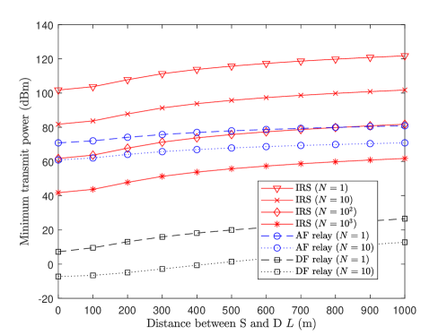
(a) Minimum transmit power versus distance $L$ under $h_{min}=100$m and $R_{0}=4$bps/Hz

(b) Energy efficiency versus achievable rate $R_{0}$ under $L=200$m and $h_{min}=100$m

(c) Energy efficiency versus $h_{min}$ under $L=200$m and $R_{0}=4$bps/Hz/W

Figure 4: Performance comparison between IRSs and full-duplex relays

Then, we compare IRSs against full-duplex relays under different sizes to draw some useful insights. It is illustrated in Fig. 4(a) that higher transmit power is required to achieve a rate $R_{0}$ as $L$ increases. Also, an IRS of size $N=10^{2}$ is needed to outperform the AF relay of size $N=1$. On the other hand, IRSs are inferior to DF relays in our setup, even when the size are extremely large, i.e., $N=10^{3}$. It is shown in Fig. 4(b) that medium size ($N=10^{2}$) is needed by IRSs to outperform AF relays. Meanwhile, large size ($N=10^{3}$) as well as high data rates ($R_{0}\geq 16$bps/Hz) are required by IRSs to outperform DF relays of size $N=1$, which coincides with the observation in[5]. Finally, the impact of $h_{min}$ is analyzed in Fig. 4(c). We can see that the energy efficiency of all relaying schemes decreases with $h_{min}$. In particular, DF relay presents a rather small reduction in energy efficiency compared with IRS and AF relay.

VI Conclusion

In this article, we analytically compare IRSs against full-duplex relays, specifically in UAV communication scenarios. Both AF and DF relaying schemes are considered for comparison. Further, 3D UAV deployment as well as transmit power are optimized. Our numerical results demonstrate that DF relays generally outperform IRSs, except in cases where the surface size of IRSs is large and data rates are high. Moreover, AF relays exhibit comparable performance to IRSs of medium size.

Appendix A Proof of Lemma 1

First, we readily have $x_{U}^{*}\in[0,L]$, $y_{U}^{*}=0$ and $h_{U}^{*}=h_{min}$ based on [12, Lemma 3]. Then the problem is simplified as finding $x_{U}\in[0,L]$ to minimize $\tilde{f}(x_{U})=(x_{U}^{2}+h_{min}^{2})((x_{U}-L)^{2}+h_{min}^{2})$. Following [16, Theorem 1], we compute the first derivative of $\tilde{f}(x_{U})$ as

$$\frac{d\tilde{f}(x_{U})}{dx_{U}} =4x_{U}^{3}-6Lx_{U}^{2}+(2L^{2}+4h_{min}^{2})x_{U}-2h_{min}^{2}L$$ (17)

$$=4\bigg{(}x_{U}-\frac{L}{2}\bigg{)}\bigg{(}\bigg{(}x_{U}-\frac{L}{2}\bigg{)}^{2}+h_{min}^{2}-\frac{L^{2}}{4}\bigg{)}.$$

1) If $L\leq 2h_{min}$, we have $\frac{d\tilde{f}(x_{U})}{dx_{U}}<0$ for $x_{U}\in[0,\frac{L}{2})$ and $\frac{d\tilde{f}(x_{U})}{dx_{U}}>0$ for $x_{U}\in(\frac{L}{2},L]$. Obviously, $x_{U}=\frac{L}{2}$ is the minimum point of $\tilde{f}(x)$;

2) On the other hand, if $L>2h_{min}$, we can obtain $x_{1,3}=\frac{L}{2}\pm\sqrt{\frac{L^{2}}{4}-h_{min}^{2}}$ and $x_{2}=\frac{L}{2}$ by setting $\frac{d\tilde{f}(x_{U})}{dx_{U}}=0$. It is observed that $\frac{d\tilde{f}(x_{U})}{dx_{U}}<0$ for $x_{U}\in[0,x_{1})\cup(x_{2},x_{3})$ and $\frac{d\tilde{f}(x_{U})}{dx_{U}}>0$ for $x_{U}\in(x_{1},x_{2})\cup(x_{3},L]$. Therefore, $x_{1}$ and $x_{3}$ are two minimum points and $\tilde{f}(x_{1})=\tilde{f}(x_{2})$ since $\tilde{f}(x_{U})$ is symmetric about $x_{U}=\frac{L}{2}$.

Appendix B Proof of Proposition 1

(14) can be directly obtained by solving $R_{IRS}=R_{0}$. In the sequel, we focus on AF and DF relays.

1) For the AF relay case, by setting $R_{AF}=R_{0}$, we shall obtain $p_{S}^{(AF)}=\frac{\rho(2^{R_{0}}-1)}{g_{SR}}p_{R}^{(AF)}+\frac{\sigma^{2}(2^{R_{0}}-1)}{N^{2}g_{SR}g_{RD}p_{R}^{(AF)}}+\frac{\sigma^{2}(2^{R_{0}}-1)}{g_{SR}}$. Therefore, $p_{S}^{(AF)}+p_{R}^{(AF)}=\frac{\rho(2^{R_{0}}-1)+g_{SR}}{g_{SR}}p_{R}^{(AF)}+\frac{\sigma^{2}(2^{R_{0}}-1)}{N^{2}g_{SR}g_{RD}p_{R}^{(AF)}}+\frac{\sigma^{2}(2^{R_{0}}-1)}{g_{SR}}\overset{(b)}{\geq}2\sqrt{\frac{\sigma^{2}(\rho(2^{R_{0}}-1)+g_{SR})(2^{R_{0}}-1)}{N^{2}g_{SR}^{2}g_{RD}}}+\frac{\sigma^{2}(2^{R_{0}}-1)}{g_{SR}}$, where $(b)$ is obtained with Cauchy inequality and the equality holds when $p_{R}^{(AF)}=\sqrt{\frac{\sigma^{2}(2^{R_{0}}-1)}{N^{2}g_{RD}(\rho(2^{R_{0}}-1)+g_{SR})}}$.

2) For the DF relay case, $\frac{p_{S}^{(DF)}g_{SR}}{\rho p_{R}^{(DF)}+\sigma^{2}}=\frac{Np_{R}^{(DF)}g_{RD}}{\sigma^{2}}$ must hold since otherwise we could further decrease $p_{S}^{(DF)}$ or $p_{R}^{(DF)}$ to achieve the equality without violating rate requirement $R_{0}$. Thereby, using $R_{DF}=R_{0}$ and after some algebra, we have $p_{S}^{(DF)}=\frac{\sigma^{2}\rho(2^{R_{0}}-1)^{2}}{Ng_{SR}g_{RD}}+\frac{\sigma^{2}(2^{R_{0}}-1)}{g_{SR}}$ and $p_{R}^{(DF)}=\frac{\sigma^{2}(2^{R_{0}}-1)}{Ng_{RD}}$.

References

- [1] C. Huang, A. Zappone, G. C. Alexandropoulos, M. Debbah, and C. Yuen, “Reconfigurable intelligent surfaces for energy efficiency in wireless communication,” IEEE transactions on wireless communications, vol. 18, no. 8, pp. 4157–4170, 2019.
- [2] Q. Wu and R. Zhang, “Towards smart and reconfigurable environment: Intelligent reflecting surface aided wireless network,” IEEE communications magazine, vol. 58, no. 1, pp. 106–112, 2019.
- [3] C. You, Z. Kang, Y. Zeng, and R. Zhang, “Enabling smart reflection in integrated air-ground wireless network: IRS meets UAV,” IEEE Wireless Communications, vol. 28, no. 6, pp. 138–144, 2021.
- [4] Y. Han, W. Tang, S. Jin, C.-K. Wen, and X. Ma, “Large intelligent surface-assisted wireless communication exploiting statistical CSI,” IEEE Transactions on Vehicular Technology, vol. 68, no. 8, pp. 8238–8242, 2019.
- [5] E. Björnson, Ö. Özdogan, and E. G. Larsson, “Intelligent reflecting surface versus decode-and-forward: How large surfaces are needed to beat relaying?” IEEE Wireless Communications Letters, vol. 9, no. 2, pp. 244–248, 2019.
- [6] Q. Wu and R. Zhang, “Intelligent reflecting surface enhanced wireless network via joint active and passive beamforming,” IEEE Transactions on Wireless Communications, vol. 18, no. 11, pp. 5394–5409, 2019.
- [7] Q. Gu, D. Wu, X. Su, J. Jin, Y. Yuan, and J. Wang, “Performance comparisons between reconfigurable intelligent surface and full/half-duplex relays,” in 2021 IEEE 94th Vehicular Technology Conference (VTC2021-Fall). IEEE, 2021, pp. 01–06.
- [8] J. Ye, A. Kammoun, and M.-S. Alouini, “Spatially-distributed RISs vs relay-assisted systems: A fair comparison,” IEEE Open Journal of the Communications Society, vol. 2, pp. 799–817, 2021.
- [9] A. Bazrafkan, M. Poposka, Z. Hadzi-Velkov, P. Popovski, and N. Zlatanov, “Performance comparison between a simple full-duplex multi-antenna relay and a passive reflecting intelligent surface,” IEEE Transactions on Wireless Communications, 2023.
- [10] C. Y. Goh and C. Y. Leow, “A comparative study of reconfigurable intelligent surfaces with relays in UAV cooperative communications,” in Advances in Information and Communication: Proceedings of the 2023 Future of Information and Communication Conference (FICC), Volume 1. Springer, 2023, pp. 100–106.
- [11] M. Di Renzo, K. Ntontin, J. Song, F. H. Danufane, X. Qian, F. Lazarakis, J. De Rosny, D.-T. Phan-Huy, O. Simeone, R. Zhang et al., “Reconfigurable intelligent surfaces vs. relaying: Differences, similarities, and performance comparison,” IEEE Open Journal of the Communications Society, vol. 1, pp. 798–807, 2020.
- [12] Y. Zeng, R. Zhang, and T. J. Lim, “Throughput maximization for UAV-enabled mobile relaying systems,” IEEE Transactions on communications, vol. 64, no. 12, pp. 4983–4996, 2016.
- [13] Q. Ding, Y. Luo, and C. Luo, “Throughput maximization of flexible duplex networks with an in-band full-duplex UAV-BS,” in ICC 2023 - IEEE International Conference on Communications, 2023, pp. 6411–6416.
- [14] Y. Chen, Y. Wang, J. Zhang, P. Zhang, and L. Hanzo, “Reconfigurable intelligent surface (RIS)-aided vehicular networks: Their protocols, resource allocation, and performance,” IEEE Vehicular Technology Magazine, vol. 17, no. 2, pp. 26–36, 2022.
- [15] A. Sabharwal, P. Schniter, D. Guo, D. W. Bliss, S. Rangarajan, and R. Wichman, “In-band full-duplex wireless: Challenges and opportunities,” IEEE Journal on selected areas in communications, vol. 32, no. 9, pp. 1637–1652, 2014.
- [16] Y. Ren, R. Zhou, X. Teng, S. Meng, M. Zhou, W. Tang, X. Li, C. Li, and S. Jin, “On deployment position of RIS in wireless communication systems: Analysis and experimental results,” IEEE Wireless Communications Letters, pp. 1–1, 2023.