A Bayes Factor Framework for Unified Parameter Estimation and Hypothesis Testing

Abstract

The Bayes factor, the data-based updating factor of the prior to posterior odds of two hypotheses, is a natural measure of statistical evidence for one hypothesis over the other. We show how Bayes factors can also be used for parameter estimation. The key idea is to consider the Bayes factor as a function of the parameter value under the null hypothesis. This ‘Bayes factor function’ is inverted to obtain point estimates (‘maximum evidence estimates’) and interval estimates (‘support intervals’), similar to how P-value functions are inverted to obtain point estimates and confidence intervals. This provides data analysts with a unified inference framework as Bayes factors (for any tested parameter value), support intervals (at any level), and point estimates can be easily read off from a plot of the Bayes factor function. This approach shares similarities but is also distinct from conventional Bayesian and frequentist approaches: It uses the Bayesian evidence calculus, but without synthesizing data and prior, and it defines statistical evidence in terms of (integrated) likelihood ratios, but also includes a natural way for dealing with nuisance parameters. Applications to real-world examples illustrate how our framework is of practical value for making make quantitative inferences.
Keywords: Bayesian inference, integrated likelihood, meta-analysis, nuisance parameters, replication studies, support interval

1 Introduction

A universal problem in data analysis is making inferences about unknown parameters of a statistical model based on observed data. In practice, data analysts are often interested in two tasks: (i) estimating the parameters (i.e., finding the most plausible value or a region of plausible values based on the observed data), and (ii) testing hypotheses related to them (i.e., using the observed data to quantify the evidence that the parameter takes a certain value). While these tasks may seem distinct, there are several statistical concepts that provide a link between the two.

In frequentist statistics, there is a duality between parameter estimation and hypothesis testing as P-values, confidence intervals, and point estimates correspond in the sense that the P-value for a tested parameter value is less than $\alpha$ if the $(1-\alpha)100\%$ confidence interval excludes that parameter value, and that the (two-sided) P-value is largest when the tested parameter value is the point estimate. The P-value function – the P-value viewed as a function of the tested parameter (for an overview see e.g., Bender et al., , 2005; Fraser, , 2019) – provides a link between these concepts. One may alternatively look at closely related quantities: One minus the two-sided P-value function known as confidence curve (Cox, , 1958; Birnbaum, , 1961), one minus the one-sided P-value function known as confidence distribution, or its derivative known as confidence density (Xie and Singh, , 2013; Schweder and Hjort, , 2016). A visualization of the P-value function, such as shown in the left plot in Figure 1, provides the observer with a wealth of information, as P-values (for any tested parameter), confidence intervals (at any level of interest), and point estimates can be easily read off. As such, P-value functions and their relatives have been deemed important measures to address common misinterpretations and misuses of P-values and confidence intervals (Greenland et al., , 2016; Infanger and Schmidt-Trucksäss, , 2019; Rafi and Greenland, , 2020; Marschner, , 2024, among others).

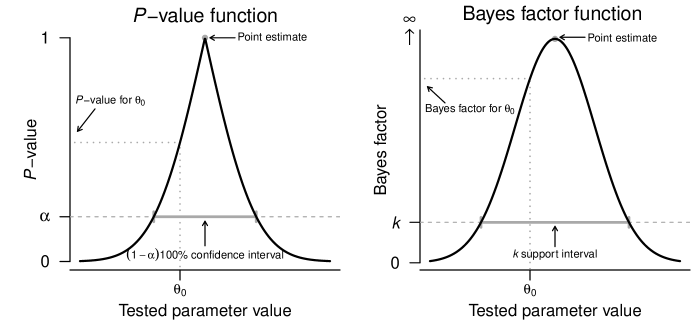
Figure 1: Examples of P-value functions and Bayes factor functions. P-value are two-sided. Bayes factors are oriented in favor of the tested parameter value over a specified alternative hypothesis (i.e., a higher Bayes factor indicates higher support for the parameter value over the alternative).

In Bayesian statistics, the posterior distribution of the unknown parameter plays a similar role to the P-value function, since point estimates (e.g., posterior modes, medians, or means), credible intervals, and posterior probabilities of hypotheses can all be derived from it. The posterior provides a synthesis of the data and the prior distribution, which can be seen as an advantage but also as a challenge in the absence of prior knowledge. In particular, for testing of hypotheses, it can be difficult to specify prior probabilities such as ‘$\Pr(\text{the treatment effect is absent})$’ and ‘$\Pr(\text{the treatment effect is present})$’.

One approach to address this issue is to report the Bayes factor (Jeffreys, , 1939; Good, , 1958; Kass and Raftery, , 1995), i.e., the updating factor of the prior to posterior odds of two hypotheses. As such, Bayes factors allow data analysts to evaluate the relative evidence for two hypotheses without depending on the prior probabilities of the hypotheses; for example, a Bayes factor can quantify the evidence for the presence or absence of a treatment effect without having to assign prior probabilities to these hypotheses (although one still has to specify a prior for the parameter under the alternative, which is challenging in itself). However, the use of Bayes factors comes at the cost of lacking an overarching concept, such as a P-value function or posterior distribution, that can provide data analyst with a coherent set of point and interval estimates. In practice, data analysts who wish to perform hypothesis testing with Bayes factors but also parameter estimation are therefore faced with a dilemma; they can either supply their Bayes factors with a posterior distribution conditional on one hypothesis being true (e.g., the posterior of a treatment effect, assuming the effect is indeed present), which can lead to contradictory conclusions with the Bayes factor (for examples, see Stone, , 1997; Wagenmakers et al., , 2022), or they can assign prior probabilities to the tested hypotheses and report a posterior averaged over both hypotheses (known as Bayesian model averaging, see e.g., Hoeting et al., , 1999; Campbell and Gustafson, , 2022), but this requires specification of prior probabilities which is highly controversial and the reason why the Bayes factor was reported in the first place rather than the posterior probabilities of the hypotheses.

Our goal is therefore to resolve this dilemma and provide a unified framework for estimation and hypothesis testing based on Bayes factors. The idea is the same as for the P-value function; we consider the Bayes factor as a function of the tested parameter. We then use this Bayes factor function to derive point estimates, interval estimates, and Bayes factors (as shown in the right plot in Figure 1), establishing a duality between hypothesis testing and parameter estimation. Our framework builds on the recently proposed Bayesian support interval (Wagenmakers et al., , 2022; Pawel et al., , 2024) and extends it with the novel concept of point estimation based on Bayes factors. We call the resulting estimate the maximum evidence estimate (MEE) – the parameter value that receives the most evidential support from the data over a specified alternative hypothesis. This provides data analysts with a unified framework for statistical inference centred around the Bayes factor.

Approaches related to the Bayes factor function have recently been proposed in the physics community under the names of ‘Bayes factor surface’ (Fowlie, , 2024) and ‘K ratio’ (Afzal et al., , 2023). Another method called ‘Bayes factor function’ has recently been proposed by Johnson et al., (2023). In this approach, Bayes factors are viewed as a function of a hyperparameter of the prior under the alternative hypothesis but for a fixed null hypothesis. We acknowledge that introducing another concept with the same name may be confusing, but we think that Bayes factor function is the most appropriate name, in analogy to P-value function.

This paper is structured as follows. In the following (Section 2), we introduce the general theory of Bayes factors, support sets, and maximum evidence estimates. We then discuss their connection to other approaches to statistical inference (Section 3). Various real data examples in Section 4 illustrate properties of the Bayes factor framework. We conclude with a discussion of the advantages, limitations, and opportunities for future research (Section 5).

2 Bayes factor function inference

Suppose we observe data $y$ with an assumed distribution with probability density/mass function $p(y\mid\theta,\psi)$ that depends on parameters $\theta\in\Theta$ and $\psi\in\Psi$, with $\theta$ being the focus parameters and $\psi$ being possible nuisance parameters. Consider two hypotheses, the null hypothesis $H_{0}\colon\theta=\theta_{0}$ postulating that $\theta$ takes a certain value $\theta_{0}$ and the alternative hypothesis $H_{1}\colon\theta\neq\theta_{0}$ postulating that $\theta$ takes a different value. A natural measure of relative evidence for the two hypotheses is the Bayes factor (Jeffreys, , 1939; Good, , 1958; Kass and Raftery, , 1995), the data-based updating factor of the prior odds of the hypotheses to their posterior odds

$$\operatorname{BF}_{01}(y;\theta_{0}) =\frac{p(H_{0}\mid y)}{p(H_{1}\mid y)}\bigg{/}\,\frac{p(H_{0})}{p(H_{1})}$$ (1a)

$$=\frac{p(y\mid H_{0})}{p(y\mid H_{1})}$$ (1b)

$$=\frac{\int_{\Psi}p(y\mid\theta_{0},\psi)p(\psi\mid H_{0})\,\mathrm{d}\psi}{\int_{\Theta}\int_{\Psi}p(y\mid\theta,\psi)\,p(\theta,\psi\mid H_{1})\,\mathrm{d}\psi\,\mathrm{d}\theta}$$ (1c)

with $p(\theta,\psi\mid H_{1})$ denoting the prior assigned to the parameters under $H_{1}$ and $p(\psi\mid H_{0})$ the prior assigned to the nuisance parameters under $H_{0}$.

As (1a) shows, the Bayes factor represents the data-based core of the Bayesian belief calculus. It remains useful even if one rejects the idea of assigning probabilities to $H_{0}$ and $H_{1}$, since this is not necessary (Goodman, , 1999). The alternative expression of the Bayes factor in equation (1b) shows that this update is dictated by the relative predictive accuracy of the two hypotheses. That is, the posterior odds of the null hypothesis $H_{0}$ increase if it outperforms the competing alternative hypothesis $H_{1}$ in predicting the data $y$, and vice versa (Good, , 1952; Gneiting and Raftery, , 2007). Finally, the last equation (1c) shows how the Bayes factor can be calculated, i.e., by dividing the likelihood of $y$ under the null value $\theta_{0}$ (possibly integrated over the prior of $\psi$ under $H_{0}$) by the likelihood of $y$ integrated over the prior of $\theta$ (and possibly $\psi$) under $H_{1}$. The priors for $\theta$ and $\psi$ may also be point priors, in which case the Bayes factor reduces to a likelihood ratio.

The idea now is to consider the Bayes factor (1) as a function of $\theta_{0}$, that is, to vary the tested parameter value (the point null hypothesis $H_{0}\colon\theta=\theta_{0}$) in order to assess the support for different parameter values over the alternative $H_{1}$, see the right plot in Figure 1 for an example. Like the P-value function, this Bayes factor function (BFF) helps to address cognitive challenges with inferential statistics (Greenland, , 2017). For example, it shifts the focus of inference from testing a single privileged null hypothesis (e.g., the hypothesis that there is no treatment effect) to an entire continuum of hypotheses. By looking at the BFF, data analysts can then identify hypotheses that receive equal or even less support from the data than the privileged one; for example, a parameter value indicating a very large treatment effect may receive equal support as the value of no treatment effect (sometimes called ‘counternull’, see Rosenthal and Rubin, , 1994).

For one- or two-dimensional focus parameters $\theta$, the BFF can be plotted as a curve or surface, respectively, so that the relative support for parameter values can be visually assessed. For higher dimensional focus parameters, this becomes more difficult and the BFF may need to be summarized in some way, which we discuss in the following.

2.1 Support sets

The BFF can be used to obtain support sets (Wagenmakers et al., , 2022) which are set-valued estimates for $\theta$ based on inverting the Bayes factor (1) similar to how P-value functions are inverted to obtain confidence sets. Specifically, a support set at support level $k>0$ is defined by

$$S_{k}=\left\{\theta_{0}:\operatorname{BF}_{01}(y;\theta_{0})\geq k\right\}$$

that is, the parameter values for which the Bayes factor indicates at least evidence of level $k$ over the specified alternative. In practice, a $k$ support set (typically an interval) is obtained from ‘cutting’ the BFF at $k$ and taking the parameter values above as part of the support set (see the right plot in Figure 1 for illustration). It may happen that for certain choices of $k$ the support set is empty because the data do not constitute relative evidence at that level.

The choice of the support level is arbitrary, just as the choice of the confidence level from a confidence set is. One may, for example, report the support level $k=1$ as it represents the tipping point at which the parameter values begin to be supported over the alternative. Conventions for Bayes factor evidence levels can also be used. For example, based on the convention from Jeffreys, (1961), a support set at level $k=10$ includes the parameter values that receive ‘strong’ relative support from the data, while a $k=1/10$ support set includes the parameter values that are at least not strongly contradicted.

2.2 The maximum evidence estimate

A natural point estimate for the unknown parameter $\theta$ based on the BFF is given by

$$\hat{\theta}_{\mathrm{ME}}=\operatorname*{arg\,max}_{\theta_{0}\in\Theta}\operatorname{BF}_{01}(y;\theta_{0}),$$

and we call it the maximum evidence estimate (MEE), since it is the parameter value for which the Bayes factor indicates the most evidence over the alternative. The associated evidence level

$$k_{\mathrm{ME}}=\operatorname{BF}_{01}(y;\hat{\theta}_{\mathrm{ME}}),$$

that is, the BFF evaluated at the MEE, quantifies the evidential value of the estimate $\hat{\theta}_{\mathrm{ME}}$ over the alternative. Evidence levels close to $k_{\mathrm{ME}}=1$ indicate that the MEE receives little support over the alternative hypothesis $H_{1}$, whereas large evidence levels $k_{\mathrm{ME}}$ indicate that the MEE receives substantial support over the alternative hypothesis $H_{1}$. A useful summary of a BFF is hence given by the MEE, its evidence level, and a support set, similar to how a P-value function may be summarized with a point estimate and confidence set.

To understand the behaviour of the MEE with increasing sample size, we may look at an approximation of the Bayes factor. Suppose that the data $y_{1:n}=\{y_{1},y_{2},\dots,y_{n}\}$ are independent and identically distributed and denote by $\hat{\psi}_{0}$ the maximizer of the log likelihood of the data under the null and by $(\hat{\theta}_{1}$, $\hat{\psi}_{1})$ the maximizer under the alternative hypothesis. Denote by $n\widehat{V}_{0}$ and $n\widehat{V}_{1}$ the modal dispersion matrices (minus the inverse of the matrix of second-order partial derivatives of the log likelihood evaluated at the corresponding maximizer). Applying a Laplace approximation to the logarithm of the BFF (O’Hagan and Forster, , 2004, equation 7.27) gives then

$$\log\operatorname{BF}_{01}(y_{1:n};\theta_{0})\approx\log\frac{p(y_{1:n}\mid\theta_{0},\hat{\psi}_{0})}{p(y_{1:n}\mid\hat{\theta}_{1},\hat{\psi}_{1})}+\frac{\dim(\theta)}{2}\log\frac{n}{2\pi}+\log\frac{p(\hat{\psi}_{0}\mid H_{0})}{p(\hat{\theta}_{1},\hat{\psi}_{1}\mid H_{1})}+\frac{1}{2}\log\frac{|\widehat{V}_{0}|}{|\widehat{V}_{1}|}.$$ (2)

To obtain the MEE, the log Bayes factor (2) needs to be maximized with respect to $\theta_{0}$. It is clear that as $\theta_{0}$ becomes more different from $\hat{\theta}_{1}$, the log normalized profile likelihood (first term) will decrease toward negative infinity, indicating evidence against the parameter value $\theta_{0}$. On the other hand, when $\theta_{0}$ is not too far from $\hat{\theta}_{1}$ the term will be about zero, so that an increasing sample size $n$ (second term) increases the log BFF toward positive infinity, indicating evidence for $\theta_{0}$. The relative accuracy of the priors (third term) and the relative dispersion (fourth term) lead to further adjustments of the BFF. For instance, when a parameter estimate is likely under the corresponding prior, this increases the evidence for corresponding hypothesis while a misspecified prior that is in conflict with the parameter estimates lowers the evidence for the corresponding hypothesis. In sum, finding the MEE corresponds approximately to maximizing the profile likelihood that is adjusted based on the accuracy of the prior of the parameters and the modal dispersion.

2.3 Example: Normal mean

Suppose we observe a single observation $y$ assumed to be sampled (at least approximately) from a normal distribution $Y\mid\theta\sim\operatorname{N}(\theta,\sigma^{2})$. Assume that $\sigma^{2}$ is known and we want to conduct inferences regarding $\theta$. This is a simple but frequently encountered scenario, for example, $y$ could be an estimated regression coefficient from a generalized linear model and $\sigma$ its estimated standard error. In the following we will consider an example from RECOVERY collaborative group, (2022). This randomised controlled trial found a reduction in mortality of patients hospitalised with COVID-19 when treated with baricitinib compared to usual care (age-adjusted log hazard ratio $y=-0.14$ with standard error $\sigma=0.064$ estimated with Cox regression). To obtain a Bayes factor for contrasting $H_{0}\colon\theta=\theta_{0}$ against $H_{1}\colon\theta\neq\theta_{0}$ we need to formulate a prior for $\theta$ under the alternative $H_{1}$. We will now discuss three choices with different characteristics shown in Table 1.

Table 1: Bayes factor function $\operatorname{BF}_{01}$, maximum evidence estimate $\hat{\theta}_{\mathrm{ME}}$, evidence value $k_{\mathrm{ME}}$, and $k$ support interval (SI) for a normal mean based on one observation $y$ from $Y\mid\theta\sim\operatorname{N}(\theta,\sigma^{2})$ with known variance $\sigma^{2}$ and for three prior distributions for $\theta$ under the alternative $H_{1}$: A normal prior (left), a normal prior centered around the parameter value of the null hypothesis $\theta_{0}$ (middle), a point prior shifted away from the parameter value of the null hypothesis $\theta_{0}$ by $d>0$ (right).

	Prior for $\theta$ under $H_{1}$
	$\theta\sim\operatorname{N}(m,v)$	$\theta\sim\operatorname{N}(\theta_{0},v)$	$\theta=\theta_{0}+d$
$\operatorname{BF}_{01}$	$\exp\left[-\frac{1}{2}\left\{\frac{(y-\theta_{0})^{2}}{\sigma^{2}}-\frac{(y-m)^{2}}{\sigma^{2}+v}\right\}\right]\sqrt{1+\frac{v}{\sigma^{2}}}$	$\exp\left[-\frac{1}{2}\left\{\frac{(y-\theta_{0})^{2}}{\sigma^{2}(1+\sigma^{2}/v)}\right\}\right]\sqrt{1+\frac{v}{\sigma^{2}}}$	$\exp\left\{\frac{2d(\theta_{0}-y)+d^{2}}{2\sigma^{2}}\right\}$
$\hat{\theta}_{\mathrm{ME}}$	$y$	$y$	non-existent
$k_{\mathrm{ME}}$	$\exp\left\{\frac{(y-m)^{2}}{2(\sigma^{2}+v)}\right\}\sqrt{1+\frac{v}{\sigma^{2}}}$	$\sqrt{1+\frac{v}{\sigma^{2}}}$	non-existent
$k$ SI	$y\pm\sigma\sqrt{\log(1+\frac{v}{\sigma^{2}})+\frac{(y-m)^{2}}{\sigma^{2}+v}-\log k^{2}}$	$y\pm\sigma\sqrt{\left\{\log(1+\frac{v}{\sigma^{2}})-\log k^{2}\right\}(1+\frac{\sigma^{2}}{v})}$	$\left[y+\frac{\sigma^{2}\log k}{d}-\frac{d}{2},\infty\right]$

Perhaps the simplest choice is a prior that does not depend on the parameter value $\theta_{0}$ of the null hypothesis, such as a normal prior with mean $m$ and variance $v$ (left column in Table 1). The hyperparameters $m$ and $v$ may be specified based on external data or based on an alternative hypothesis of interest (e.g., the prior mean $m$ could be set to a minimum clinically important treatment effect and $v$ could be set to zero to obtain a point prior as typically used in a power analysis). RECOVERY collaborative group, (2022) reported a meta-analytic log hazard ratio and standard error based on eight previous trials, which we now use to set the prior mean and variance to $m=-0.56$ and $v=0.12^{2}$, see Figure 2 for the resulting BFF (orange). In this case, the MEE is given by $\hat{\theta}_{\mathrm{ME}}=y=-0.14$ with the support interval centered around it. Due to the apparent conflict between the observed data and the specified prior under the alternative, the $k=1$ support interval spans an wide range from $-0.35$ to $0.08$, indicating that very beneficial up to slightly harmful treatment effects are supported by the data over the alternative.

The formulae in Table 1 (left column) show that as the prior mean $m$ becomes closer to the observed data $y$, the evidence level $k_{\mathrm{ME}}$ decreases and the support interval becomes narrower. This is because an alternative closer to the data clearly has better predictive accuracy of the data than an alternative further away, and thus fewer point null hypotheses can outpredict it. Figure 2 illustrates this phenomenon with another prior distributions (one with mean at the observed log hazard ratio $y=-0.14$, the blue BFF). The BFF has its mode still at the observed log hazard ratio estimate but shows a far narrower $k=1$ support interval from $-0.22$ to $-0.06$ than the orange BFF with the mean $m=-0.56$ based on the eight previous trials.

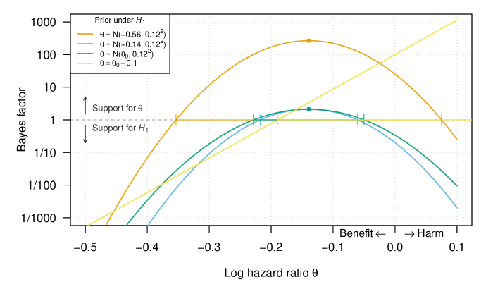
Figure 2: Bayes factor function, MEE, and $k=1$ support interval for a log hazard ratio $\theta$ based on estimated log hazard ratio $y=-0.14$ with standard error $\sigma=0.064$ from the RECOVERY trial (RECOVERY collaborative group, , 2022) for different prior distributions for the $\theta$ under the alternative $H_{1}$. A normal likelihood $Y\mid\theta\sim\operatorname{N}(\theta,\sigma^{2}_{i})$ is assumed for the data.

Another approach to formulating a prior distribution for $\theta$ under the alternative commonly suggested in ‘objective’ Bayes theories is to center the prior around the tested parameter value $\theta_{0}$ (Jeffreys, , 1961; Berger and Delampady, , 1987; Kass and Wasserman, , 1995). For example, one can specify a normal prior with mean at the null value $\theta_{0}$ (middle column in Table 1). Thus, the resulting BFF varies both the null and the alternative, unlike the BFF based on the ‘global’ normal prior with fixed mean $m$. As a result, the interpretation of the BFF is different: For such a ‘local’ normal prior, the BFF quantifies the support of parameter values over alternative parameter values in a neighborhood around them. As for the global normal prior, the MEE based on the local normal prior is given by $\hat{\theta}_{\mathrm{ME}}=y$ and support intervals are centered around it, but the associated, Bayes factor, evidence level and support interval are different. Figure 2 illustrates that when the mean $m$ of a global normal prior is too different from the observed data $y$ (as in the case of the orange BFF, where the prior was specified based on the eight previous trials), the $k=1$ support interval based on the local prior with the same variance is narrower. On the other hand, when the mean $m$ of the global prior is equal to the data (blue BFF), the support interval based on the local prior is wider.

The last prior in the right most column of Table 1 represents a point prior shifted from the null value $\theta_{0}$ by $d>0$. The prior is again ‘local’ in the sense that it is different for each tested parameter value of the null hypothesis $\theta_{0}$, and as such encodes an alternative hypothesis that the log hazard ratio is greater than the tested parameter value. However, this leads to an ever-increasing BFF, see Figure 2 for a numerical illustration. As a result, the MEE and its evidence level do not exist, while the support interval still exists but its right limit extends to infinity. Although such a prior seems unrealistic, the example demonstrates that a poorly chosen prior can lead to pathological behavior of the resulting BFF.

2.4 Choice of the prior

As the previous example showed, the prior assigned to the parameters under the alternative has a substantial impact on BFF inference. This ‘sensitivity’ of Bayes factors to prior distributions enables data analysts to accurately quantify the support of parameter values over informative alternative hypotheses when they are available, but poses a challenge in their absence (Kass and Raftery, , 1995). Various approaches have been proposed to deal with this issue, for example, ‘default’ or ‘objective’ prior distributions (Bayarri et al., , 2012; Consonni et al., , 2018), reverse-Bayes analysis (Held et al., , 2022), prior elicitation (O’Hagan, , 2019), or sensitivity analysis (Franck and Gramacy, , 2019), all with advantages and disadvantages. Here we will not reiterate general considerations on prior specification for Bayes factors (see e.g., Section 5 in Kass and Raftery, , 1995) but focus on specific considerations related to BFFs.

As in other Bayes factor applications, BFFs are only unambiguously defined if priors for focus parameters are proper under the alternative $H_{1}$ (i.e., integrate to one), whereas priors for nuisance parameters may be improper as long as the same prior is assigned under both the null $H_{0}$ and the alternative $H_{1}$ so that arbitrary constants cancel out. A general distinction can be made between global priors, which do not depend on the value of $\theta_{0}$ under the null hypothesis and local priors, which do. In the latter case, the interpretation of the BFF is more intricate, since for each parameter value the BFF quantifies the support over a different alternative. For a more natural interpretation, global priors may hence be preferred over local priors. At the same time, local priors correspond to the typical use of ‘default’ Bayes factors, which is to center the prior around $\theta_{0}$, and as such may be preferred in the same situations where default Bayes factors would be used.

Finally, it is usually advisable to report sensitivity analyses for plausible ranges of priors, to assess the robustness of the conclusions. A convenient visual sensitivity analysis is, for example, to plot different BFFs resulting from different prior specifications, as shown in Figure 2. One can go a step further and use a ‘reverse-Bayes‘ approach (Good, , 1950; Held et al., , 2022), which involves systematically determining the prior that represents the tipping point and changes the conclusions of the analysis. Data analysts can then reason about whether or not such a prior is plausible in the light of external knowledge and data.

2.5 Sequential analysis

An attractive property of Bayesian inference is that it provides a coherent way to analyze data that come in batches. That is, the same posterior distribution is obtained regardless of whether all data are analyzed at once, or whether the posterior distribution based on one batch is used as the prior for the other.

If we have two batches $y_{1}$ and $y_{2}$, the BFF based on both batches is

$$\operatorname{BF}_{01}(y_{1:2};\theta_{0}) =\operatorname{BF}_{01}(y_{1};\theta_{0})\times\operatorname{BF}_{01}(y_{2}\mid y_{1};\theta_{0})$$

where

$$\operatorname{BF}_{01}(y_{2}\mid y_{1};\theta_{0}) =\frac{\int_{\Psi}p(y_{2}\mid\theta_{0},\psi)\,p(\psi\mid y_{1},H_{0})\,\mathrm{d}\psi}{\int_{\Theta}\int_{\Psi}p(y_{2}\mid\theta,\psi)\,p(\theta,\psi\mid y_{1},H_{1})\,\mathrm{d}\psi\,\mathrm{d}\theta}$$

is the partial Bayes factor obtained from using the posterior distributions under the null $p(\psi\mid y_{1},H_{0})$ and under the alternative $p(\theta,\psi\mid y_{1},H_{1})$ based on the first batch $y_{1}$ to compute the Bayes factor based on the second batch $y_{2}$ (O’Hagan and Forster, , 2004, p.186). This result generalizes to more than two batches by

$$\operatorname{BF}_{01}(y_{1:n};\theta_{0}) =\operatorname{BF}_{01}(y_{1};\theta_{0})\times\prod_{i=2}^{n}\operatorname{BF}_{01}(y_{i}\mid y_{1:(i-1)};\theta_{0}),$$

that is, a BFF based on all the available data can be obtained by multiplying the BFF based on the previous batches by the partial Bayes factor based on the current batch. Thus, like ordinary Bayesian inference with posterior distributions, BFF inference is sequentially coherent.

2.6 Asymptotic behaviour of the Bayes factor function

It is of interest to understand the asymptotic behaviour of the BFF, that is, how does the BFF (and quantities derived from it) behave as more data are generated under a certain ‘true’ hypothesis? It is well-known that Bayes factors are consistent in the sense that when the data are generated under one of the contrasted hypotheses, the Bayes factor tends to overwhelmingly favour that hypothesis over the alternative as more data are generated, i.e., go to zero or infinity, depending on the orientation of the Bayes factor (see e.g., Kass and Vaidyanathan, , 1992; Gelfand and Dey, , 1994; Dawid, , 2011). Since the BFF is nothing else than the Bayes factor evaluated for various null hypotheses, this consistency property carries over to the BFF. That is, as more data are generated from the true model with parameter $\theta_{*}$, the BFF at $\theta_{0}=\theta_{*}$ will go to infinity, while the BFF at $\theta_{0}\neq\theta_{*}$ will go to zero.

As a concrete example where the distribution of the BFF can be derived in closed-form, consider again inference about a normal mean based on data $Y\mid\theta\sim\operatorname{N}(\theta,\kappa^{2}/n)$, where $\kappa^{2}$ denotes a unit-variance and $n$ the sample size. The logarithm of the BFF based on a normal prior $\theta\mid H_{1}\sim\operatorname{N}(m,v)$ can then be written as

$$\log\operatorname{BF}_{01}(Y;\theta_{0}) =\frac{1}{2}\left[\log\left(1+\frac{n\,v}{\kappa^{2}}\right)+\frac{(\theta_{0}-m)^{2}}{v}-\left\{Y-\frac{(\theta_{0}-m)\kappa^{2}}{n\,v}-\theta_{0}\right\}^{2}\frac{v\,n}{\kappa^{2}(v+\kappa^{2}/n)}\right].$$ (3)

Hence, when the data are generated from $Y\mid\theta_{*}\sim\operatorname{N}(\theta_{*},\kappa^{2}/n)$ with true mean $\theta_{*}$, we have that

$$\left\{Y-\frac{(\theta_{0}-m)\kappa^{2}}{n\,v}-\theta_{0}\right\}^{2}\frac{n}{\kappa^{2}}\sim\chi^{2}_{1,\lambda}$$

with non-centrality parameter $\lambda=n\left\{\theta_{*}-\frac{(\theta_{0}-m)\kappa^{2}}{n\,v}-\theta_{0}\right\}^{2}/\kappa^{2}.$ Thus, by rearranging terms in (3), we can compute the probability that the Bayes factor is below some threshold $\gamma$ by

$$\Pr\{\operatorname{BF}_{01}(Y;\theta_{0})\leq\gamma\mid\theta_{*}\}=1-\Pr(\chi_{1,\lambda}^{2}\leq X)$$

with

$$X=\left\{\log\left(1+\frac{n\,v}{\kappa^{2}}\right)+\frac{(\theta_{0}-m)^{2}}{v}-2\log\gamma\right\}\left(1+\frac{\kappa^{2}}{v\,n}\right).$$

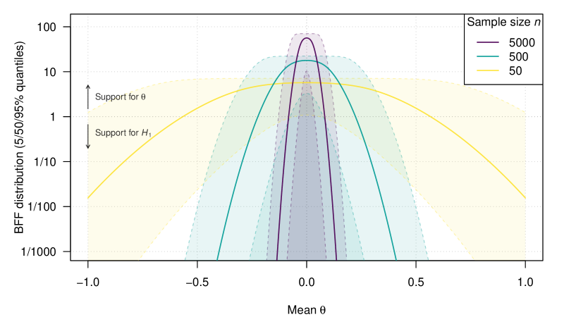
Figure 3: Distribution of the BFF for different sample sizes. A data model $Y\mid\theta\sim\operatorname{N}(\theta,\kappa^{2}/n)$ is assumed and data are generated from a true mean $\theta_{*}=0$ and unit-variance $\kappa^{2}=4$. The BFF is based on a local normal prior $\theta\mid H_{1}\sim\operatorname{N}(\theta_{0},v=4)$ assigned to $\theta$ under the alternative.

Figure 3 shows the distribution of the BFF for different sample sizes, a true mean of $\theta_{*}=0$, a unit-variance of $\kappa^{2}=4$, and with a local normal prior with the same unit variance (a unit-information prior, see Kass and Wasserman, , 1995) specified under the alternative. We see that as the sample size increases, the distribution of the BFF at the true mean shifts toward larger values, indicating more evidence for the true mean, as it should. On the other hand, the further away the BFF is evaluated from the true mean, the more its distribution shifts toward smaller values, indicating increasing evidence for the alternative, as it should.

3 Connection to other inference frameworks

We will now explore connections of BFF inference to other inference frameworks.

3.1 Maximum integrated likelihood

In typical situation where a division of the null’s marginal likelihood $p(y\mid H_{0})$ by the alternative’s marginal likelihood $p(y\mid H_{1})$ does not change the maximizer of the null’s marginal likelihood $p(y\mid H_{0})$, the MEE can be obtained by maximizing $p(y\mid H_{0})$ without reference to an alternative $H_{1}$. This is, for instance, the case when a global prior (a prior that does not depend on $\theta_{0}$) is assigned to $\theta$ under the alternative, or also in the case of the local normal prior that is centered around $\theta_{0}$ from the previous example. The MEE is then equivalent to the maximizer of the integrated likelihood

$$\hat{\theta}_{\mathrm{MIL}}=\operatorname*{arg\,max}_{\theta\in\Theta}\int_{\Psi}p(y\mid\theta,\psi)\,p(\psi\mid H_{0})\,\mathrm{d}\psi,$$

based on prior $p(\psi\mid H_{0})$ assigned to the nuisance parameters (see e.g., Kalbfleisch and Sprott, , 1970; Basu, , 1977; Berger et al., , 1999; Royall, , 1997; Severini, , 2007). When there are no nuisance parameters, the MEE reduces to the ordinary maximum likelihood estimate.

To consider a concrete example, assume a sample of $n$ normal random variables $Y_{1},\dots,Y_{n}\mid\theta,\sigma^{2}\overset{i.i.d.}{\sim}\operatorname{N}(\mu,\sigma^{2})$. Suppose that $\sigma^{2}$ is the focus and $\mu$ the nuisance parameter, and that an improper uniform prior $p(\mu\mid H_{0})=1$ is assigned to $\mu$. The intergrated likelihood of an observed sample $y_{1},\dots,y_{n}$ is then

$$p(y_{1},\dots,y_{n}\mid\sigma^{2})=(2\pi\sigma^{2})^{-(n-1)/2}\,n^{-1/2}\,\exp\left\{\frac{-\sum_{i=1}^{n}(y_{i}-\bar{y})^{2}}{2\sigma^{2}}\right\}$$

and maximizing it leads to the sample variance (REML) estimate of the variance

$$\hat{\sigma}^{2}_{\mathrm{MIL}}=\frac{\sum_{i=1}^{n}(y_{i}-\bar{y})^{2}}{n-1}.$$

The same MEE is obtained when the prior $p(\mu,\sigma^{2}\mid H_{1})$ does not depend on the value of the variance under $H_{0}$ as the denominator of the Bayes factor is simply a multiplicative factor that does not change its maximum. This shows that REML and MIL estimates can also be motivated from a Bayesian evidence perspective which complements the well-established connections between REML estimation and marginal posterior estimation based on flat priors for the nuisance parameters (Harville, , 1974; Laird and Ware, , 1982). It is reassuring that different methods produce the same estimate in these situations. However, the important difference between these methods is the motivation and interpretation of the resulting estimate – the MEE represents a natural estimate for $\theta$ because it is the parameter value for which the data provide the most evidence over an alternative hypothesis, while the (integrated) maximum likelihood estimate is defined without reference to alternatives.

3.2 Likelihoodist inference

The likelihoodist school of statistical inference (Barnard, , 1949; Edwards, , 1971; Royall, , 1997; Blume, , 2002) rejects the use of prior distributions to formulate alternatives or to eliminate nuisance parameters, but it also shares features with the BFF paradigm. That is, if point priors are assigned to the parameters, the Bayes factor reduces to a likelihood ratio which is the evidence measure used by likelihoodists. For this reason, BFF inferences correspond to likelihoodist inferences if the Bayesian and likelihoodist agree on the used point priors.

However, there is disagreement when it comes to the use of support sets. When there are no nuisance parameters, likelihoodists define their support sets based on the relative likelihood

$$L(\theta)=\frac{p(y\mid\theta)}{p(y\mid\hat{\theta}_{\textrm{ML}})}$$ (4)

where $\hat{\theta}_{\textrm{ML}}$ is the maximum likelihood estimate. For example, Royall, (1997) recommended reporting the set of parameter values with relative likelihood greater than $k=1/8$ (at most ‘strong’ evidence against them) or $k=1/32$ (at most ‘quite strong’ evidence against them). From a Bayesian perspective, using the observed maximum likelihood estimate as a prior under the alternative seems to hardly represent genuine prior knowledge or an alternative theory, but rather a cherry-picked alternative that gives to the most biased assessment of support for the alternative (Berger and Sellke, , 1987).

3.3 Frequentist inference

The relative likelihood (4) serves as an important basis for frequentist statistics since under the null hypothesis $-2\log L(\theta_{0})$ has an asymptotic chi-squared distribution with $\dim(\theta)$ degrees of freedom. Frequentists thus also use relative likelihoods but merely as a test statistic.

Another connection between frequentist and BFF inference is given by the ‘universal bound’ (Kerridge, , 1963; Robbins, , 1970; Royall, , 1997), which bounds the frequentist probability of obtaining misleading Bayesian evidence. That is, when data are generated under $H_{0}:\theta=\theta_{0}$, the probability of obtaining a Bayes factor $\operatorname{BF}_{01}$ less than $k<1$ is at most $k$ for any prior under the alternative

$$\Pr\{\operatorname{BF}_{01}(y)\leq k\mid H_{0}\}\leq k.$$

If there are nuisance parameters, the bound holds only marginalized over the prior of the nuisance parameters. For the bound to hold in a strict sense (i.e., for every possible value of the nuisance parameter), special priors must be assigned to them (Hendriksen et al., , 2021; Grünwald et al., , 2024).

The universal bound can thus be used to transform BFFs into conservative P-values and confidence sets, e.g., a $k=1/20$ support set obtained from a BFF corresponds to a 95% conservative confidence set and $p=\min\{\operatorname{BF}_{01},1\}$ corresponds to a conservative $P$-value. Remarkably, the bound holds without adjustment even when the data collection is continuously monitored and stopped as soon as evidence against $H_{0}$ is found (Robbins, , 1970). However, it is important to note that P-values and confidence sets obtained in this way are usually much more conservative than ordinary ones which are calibrated to have exact type I error rate and coverage, respectively. Finally, if the data model is misspecified, the bound is obviously invalid.

3.4 Bayesian inference

The BFF can, under certain conditions, be transformed into a Bayesian posterior distribution. Specifically, assuming that the priors for the nuisance parameters satisfy $p(\psi\mid H_{0})=p(\psi\mid\theta=\theta_{0},H_{1})$, the Bayes factor can be represented as the ratio of marginal posterior to prior density evaluated at the tested parameter value (known as Savage-Dickey density ratio, see e.g., Dickey, , 1971; Verdinelli and Wasserman, , 1995; Wagenmakers et al., , 2010). Hence, the posterior can be obtained by multiplying the BFF with the prior

$$p(\theta\mid y,H_{1})=\underbrace{\frac{p(y\mid\theta,H_{1})}{p(y\mid H_{1})}}_{=\operatorname{BF}_{01}(y;\theta)}\times p(\theta\mid H_{1}).$$ (5)

It is, however, important to emphasize that BFFs based on priors under the alternative that depend on the null (e.g., commonly used ‘local’ normal or Cauchy priors that are centered around $\theta_{0}$) cannot be transformed to a genuine posterior distribution in this way, but multiplication with the prior will result in a different posterior for every $\theta$.

Since, under certain regularity conditions, the posterior is asymptotically normally distributed around the maximum likelihood estimate (Bernardo and Smith, , 2000, chapter 5.3), we can conclude that whenever these conditions are satisfied and the BFF has the Savage-Dickey density ratio representation (5), the BFF is asymptotically given by the asymptotic posterior normal density divided by the prior density, both evaluated at $\theta_{0}$. The posterior, and hence also the BFF, will become more concentrated around the true parameter $\theta_{*}$ as more data are generated, giving another intuition about the consistency property of Bayes factors.

The Savage-Dickey density ratio (5) also provides a convenient way to compute BFFs: One of the many programs for computing Bayesian posterior distributions, such as Stan (Carpenter et al., , 2017) or INLA (Rue et al., , 2009), can be used to compute a posterior density, which can then be divided by the prior density to obtain a BFF. The caveat is again that this only works for global priors under the alternative and with the same prior assigned to the nuisance parameters under the null and alternative.

The relationship between the posterior and the BFF also exposes its connection to another Bayesian inference quantity – the relative belief ratio

$$\mathrm{RB}(\theta\mid H_{1})=\underbrace{\frac{p(\theta\mid y,H_{1})}{p(\theta\mid H_{1})}}_{=\operatorname{BF}_{01}(y;\theta)},$$ (6)

see e.g., Evans, (2015). This quantity is the updating factor of the prior to the posterior density/mass function, and is related to the Bayes factor via the aforementioned mentioned Savage-Dickey density ratio. An estimation and testing framework centred on the relative belief ratio was developed by Evans, (1997). The parameter value that maximizes the relative belief ratio was termed the least relative surprisal estimate, later also referred to as maximum relative belief estimate (Evans, , 2015). Clearly this estimate is equivalent to the MEE whenever the BFF and relative belief ratio coincide. Evans, (1997) also defined a $\delta\times 100\%$ relative surprise region, which is the set of parameter values with $\delta\times 100\%$ posterior probability and with highest relative belief ratios among all such sets. Similarly, Shalloway, (2014) defined an evidentiary credible region which is equivalent to the relative surprise region, but motivated by information theory. While both are closely related to the support set via the Savage-Dickey density ratio, they differ from the support set in that they are defined by posterior probabilities and not by evidence, the ordering induced by the relative belief ratio merely provides a rule to chose among all credible sets (Wagenmakers et al., , 2022). Thus, a relative surprise region may contain parameter values that are not supported by the data. For this reason, Evans, (2015) defined yet another type of region, a $k$ plausible region which contains parameter values with a relative belief ratio of at least $k$ and as such coincides with the $k$ support set whenever the Savage-Dickey density representation applies to the BFF and when a global prior is chosen for $\theta$ under the alternative.

4 Applications

We will now apply BFF inference to several real-world examples.

4.1 Binomial proportion

Bartoš et al., (2023) conducted a study to test the hypothesis that fair coins tend to land on the same side as they started slightly more often (with a probability of about 0.51). This hypothesis was formulated by Diaconis et al., (2007) based on a physical model of coin flipping. During the course of the study, 48 participants contributed to the collection of $n=350^{\prime}757$ coin flips among which $y=178^{\prime}078$ landed on the same side as they started.

We will now assume a binomial data model $Y\mid\theta\sim\operatorname{Bin}(n,\theta)$ and conduct inferences regarding the unknown probability $\theta$. In their pre-registered analysis, Bartoš et al., (2023) specified a truncated beta prior for the probability $\theta$ under the alternative ($\theta\mid H_{1}\sim\operatorname{Beta}(a,b)_{[l,u]}$). Based on this prior, the Bayes factor for testing $H_{0}\colon\theta=\theta_{0}$ against $H_{1}\colon\theta\neq\theta_{0}$ is

$$\operatorname{BF}_{01}(y;\theta_{o})=\frac{\theta_{0}^{y}\,(1-\theta_{0})^{n-y}}{\operatorname{{B}}(a+y,b+n-y)/\operatorname{{B}}(a,b)}\times\frac{I_{u}(a,b)-I_{l}(a,b)}{I_{u}(a+y,b+n-y)-I_{l}(a+y,b+n-y)}$$

with the beta function $\operatorname{{B}}(a,b)=\int_{0}^{1}t^{a-1}\,(1-t)^{b-1}\,\mathrm{d}t$ and the incomplete regularized beta function $I_{x}(a,b)=\{\int_{0}^{x}t^{a-1}\,(1-t)^{b-1}\,\mathrm{d}t\}/\operatorname{{B}}(a,b)$. Specifically, Bartoš et al., (2023) assigned the hyperparameters $a=5100,b=4900,l=0.5,u=1$ to instantiate an alternative hypothesis that closely aligns with the theoretical prediction from Diaconis et al., (2007) of a 0.51 probability with slight uncertainty around it.

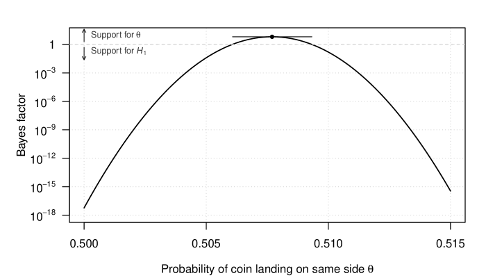
Figure 4: Bayes factor function analysis of data from Bartoš et al., (2023). Among $n=350^{\prime}757$ coin flips, $y=178^{\prime}078$ landed on the same side as they started. A beta prior tightly concentrated around the theoretically predicted probability of 0.51 is assigned to the probability under the alternative ($\theta\mid H_{1}\sim\operatorname{Beta}(5100,4900)_{[0.5,1]}$).

Figure 4 shows the resulting BFF for a range of probabilities from 0.5 to 0.515. Looking at the BFF evaluated at $\theta=0.5$, we can see the finding reported by Bartoš et al., (2023): There is extreme evidence ($\operatorname{BF}_{01}=1/(1.71\times 10^{17})$) against $\theta=0.5$ and in favour of the alternative concentrated around $\theta=0.51$. This result hence provides decisive evidence for the theory from Diaconis et al., (2007) over the hypothesis that coins tend to land on the same side with equal probability. However, the BFF framework permits further insights. For example, we can see that all probability values up to about 0.504 and all values larger than 0.512 are decisively refuted by the data, each having an associated Bayes factor below $10^{-3}$. Furthermore, the $k=1$ support interval from 0.506 to 0.509 shows the probability values that are better supported by the data than the specified alternative, which excludes the theoretically predicted $\theta=0.51$. The MEE at $\hat{\theta}_{\mathrm{ME}}=0.508$ is the best supported value, with $k_{\mathrm{ME}}=6.51$ indicating substantial evidence over the alternative concentrated around 0.51.

4.2 Meta-analysis

The previous analysis assumed that coin flips were independent among participants and trials. The top left plot in Figure 5 shows that this assumption seems violated as the estimated probabilities that a coin lands on the same side for each of the $n=48$ study participants are clearly heterogeneous. This suggests that the analysis should be modified to account for heterogeneity. In the following, we will therefore synthesize these estimates while accounting for heterogeneity with a meta-analysis, as Bartoš et al., (2023) did.

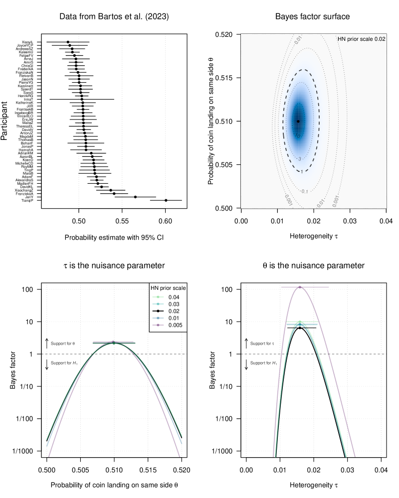
Figure 5: Bayes factor analysis of coin flipping experiments from Bartoš et al., (2023), taking into account between-participant heterogeneity. The product of a truncated beta prior ($\theta\mid H_{1}\sim\operatorname{Beta}(5100,4900)_{[0.5,1]}$) for $\theta$ and a half-normal prior with scale 0.02 for $\tau$ are assigned under the alternative $H_{1}$. The same priors are assumed when the parameters are nuisance parameters under $H_{0}$ (bottom plots). The bottom plots also show the BFF for other scale parameters of the half-normal prior.

Suppose we have $i=1,\dots,n$ estimates $y_{i}$ with (assumed to be known) standard errors $\sigma_{i}$. The estimates are assumed to be normally distributed around a participant specific true probability $\theta_{i}$, i.e.,

$$y_{i}\mid\theta_{i},\sigma^{2}_{i} \sim\operatorname{N}(\theta_{i},\sigma^{2}_{i})$$

$$\theta_{i}\mid\theta,\tau^{2} \sim\operatorname{N}(\theta,\tau^{2}).$$

Marginalized over the participant specific probabilities, the distribution of an estimate is then

$$y_{i}\mid\theta,\tau,\sigma^{2}_{i} \sim\operatorname{N}(\theta,\sigma^{2}_{i}+\tau^{2}).$$

There are two unknown parameters, $\theta$ and $\tau$. The mean $\theta$ quantifies the average probability across participants, while the heterogeneity standard deviation $\tau$ quantifies the heterogeneity of these probabilities. The Bayes factor for testing $H_{0}\colon\theta=\theta_{0},\tau=\tau_{0}$ against $H_{1}\colon\theta\neq\theta_{0},\tau\neq\tau_{0}$ is then given by

$$\operatorname{BF}_{01}(y_{1},\dots,y_{n};\theta_{0},\tau_{0})=\frac{\prod_{i}^{n}\operatorname{N}(y_{i}\mid\theta_{0},\tau_{0}^{2})}{\int_{0}^{\infty}\int_{-\infty}^{+\infty}\prod_{i}^{n}\operatorname{N}(y_{i}\mid\theta,\tau^{2})\,p(\theta,\tau\mid H_{1})\,\mathrm{d}\theta\,\mathrm{d}\tau}$$

with $\operatorname{N}(x\mid m,v)$ denoting the normal density with mean $m$ and variance $v$ evaluated at $x$.

As in the previous analysis we assigned a $\theta\mid H_{1}\sim\operatorname{Beta}(5100,4900)_{[0.5,1]}$ prior to the average probability $\theta$ under the alternative $H_{1}$. In addition, we assigned a half-normal prior $p(\tau\mid H_{1})=\sqrt{2/\pi}\,\exp\{-\tau^{2}/(2\,s^{2})\}/s$ to the heterogeneity standard deviation $\tau$, and assumed it to be independent of $\theta$. Half-normal priors are commonly used in meta-analysis due to their simplicity and desirable properties such as nearly uniform behavior around zero $\tau=0$ (see e.g., Röver et al., , 2021). We choose a scale $s=0.02$ because the resulting prior gives $95\%$ probability to $\tau$ values smaller than 0.04, thus encoding the possibility of no heterogeneity (all true participant probabilities are the same when $\tau=0$) up to small amounts of heterogeneity (the true participant probabilities differ by a few percentage points). BFFs for priors with smaller or larger scale parameters are also shown in Figure 5 as sensitivity analyses.

The top-right plot in Figure 5 shows the BFF in a two-dimensional surface when both parameters are considered as focus parameters. In contrast to the analysis that ignored between-participant heterogeneity, we see that the MEE for the average probability ($\hat{\theta}_{\mathrm{ME}}=0.51$) is now consistent with the theoretical prediction of Diaconis et al., (2007). In addition, the MEE for the heterogeneity standard deviation ($\hat{\tau}_{\mathrm{ME}}=0.016$) suggests small but non-negligible heterogeneity. This MEE receives strong support over the alternative ($k_{\mathrm{ME}}=14$). The relatively concentrated $k=1$ support region indicates that probabilities from around 0.505 to 0.515 along with heterogeneity standard deviations from 0.012 to 0.021 are supported by the data over the alternative. Finally, the BFF shows that probabilities of $\theta=0.5$ and no heterogeneity $\tau=0$ are clearly refuted by the data over the alternative ($\log\operatorname{BF}_{01}=-1.81\times 10^{5}$).

The two bottom plots in Figure 5 show BFFs when either $\tau$ or $\theta$ is considered as nuisance parameter. In both cases, the same prior as for the alternative $H_{1}$ was assigned to the corresponding nuisance parameter under $H_{0}$. In addition, BFFs for other choices of the scale parameter of the half-normal prior were computed to assess the sensitivity of the results to this choice. We see that the two marginal MEEs ($\hat{\theta}_{\mathrm{ME}}=0.51$ and $\hat{\tau}_{\mathrm{ME}}=0.016$) align with the joint MEEs, but their evidence values ($k_{\mathrm{ME}}=2.2$ and $k_{\mathrm{ME}}=6.4$, respectively) indicate less support over the alternative than for the joint one. Finally, looking at the colored BFFs obtained by changing the scale parameter of the half-normal prior assigned to $\tau$, we see that the scale has little effect on inferences about the probability $\theta$, but a more pronounced effect on inferences about $\tau$. For the latter parameter, increasing the scale of the prior does not seem to change the BFF too much, while decreasing the scale to a value of $s=0.005$ dramatically increases the height of the BFF, increasing the support of the MEE and surrounding values over the alternative. This seems reasonable, since the data show clear signs of heterogeneity, while a prior with such a small scale would predict almost none. In sum, the BFF analysis suggests that, on average, coins tend to land on the same side with probability $\theta=0.51$ in accordance with the hypothesis from Diaconis et al., (2007). At the same time, there seems to be considerable between-flipper heterogeneity.

4.3 Replication studies

In a replication study, researchers repeat an original study as closely as possible in order to assess whether consistent results can be obtained (National Academies of Sciences, Engineering, and Medicine, , 2019). Various types of Bayes factor approaches have been proposed to quantify the degree to which a replication study has replicated an original study (Verhagen and Wagenmakers, , 2014; Ly et al., , 2018; Harms, , 2019; Pawel and Held, , 2022; Pawel et al., , 2023). A common idea is that the posterior distribution of the unknown parameters based on the data from the original study is used as the prior distribution in the analysis of the replication data. If the replication data support this prior distribution, this suggests replication success. We will now show how this idea translates to analyzing replication studies with BFFs.

Suppose that original and replication study provide effect estimates $y_{o}$ and $y_{r}$ with standard errors $\sigma_{o}$ and $\sigma_{r}$, respectively. Each is supposed to be normally distributed around a common underlying effect size $\theta$ with (assumed to be known) variance equal to its squared standard error, i.e., $y_{i}\mid\theta\sim\operatorname{N}(\theta,\sigma^{2}_{i})$ for $i\in\{o,r\}$. A ‘replication BFF’ may then be obtained by using the replication data to contrast the null hypothesis $H_{0}\colon\theta=\theta_{0}$ to the alternative $H_{1}\colon\theta\sim\operatorname{N}(y_{o},\sigma^{2}_{o})$, where the prior under the alternative is the posterior distribution of $\theta$ based on the original data and a flat prior for $\theta$ (Verhagen and Wagenmakers, , 2014). As such, the replication Bayes factor represents a special case of the ‘partial Bayes factor‘ (O’Hagan and Forster, , 2004, p.186). This leads to the following BFF

$$\operatorname{BF}_{01}(y_{r};\theta_{0})=\sqrt{1+\frac{\sigma^{2}_{o}}{\sigma^{2}_{r}}}\,\exp\left[-\frac{1}{2}\left\{\frac{(y_{r}-\theta_{0})^{2}}{\sigma^{2}_{r}}-\frac{(y_{r}-y_{o})^{2}}{\sigma^{2}_{r}+\sigma^{2}_{o}}\right\}\right]$$

with MEE at the replication effect estimate $\hat{\theta}_{\mathrm{ME}}=y_{r}$, evidence value

$$k_{\mathrm{ME}}=\sqrt{1+\frac{\sigma^{2}_{o}}{\sigma^{2}_{r}}}\,\exp\left\{\frac{(y_{r}-y_{o})^{2}}{2(\sigma_{o}^{2}+\sigma^{2}_{r})}\right\},$$

and $k$ support interval

$$y_{r}\pm\sigma_{r}\sqrt{\log\left(1+\frac{\sigma^{2}_{o}}{\sigma^{2}_{r}}\right)+\frac{(y_{r}-y_{0})^{2}}{\sigma^{2}_{r}+\sigma^{2}_{o}}-\log k^{2}}.$$

We will now demonstrate application of the replication BFF by reanalyzing data from three replication studies that were part of the large-scale replication project in the social-behavioral sciences (Protzko et al., , 2023). The original experiment termed “Labels” found the following central result:

“When a researcher uses a label to describe people who hold a certain opinion, he or she is interpreted as disagreeing with that opinion when a negative label is used and agreeing with that opinion when a positive label is used.” Protzko et al., (2023, p. 312)

which was based on an estimated standardized mean difference $y_{o}=0.205$ with standard error $\sigma_{o}=0.051$. The replication studies conducted in three other labs found a smaller, a similar, and a much larger effect estimate ($y_{ri}\in\{0.09,0.205,0.435\}$ with standard errors $\sigma_{ri}\in\{0.052,0.057,0.044\}$, respectively).

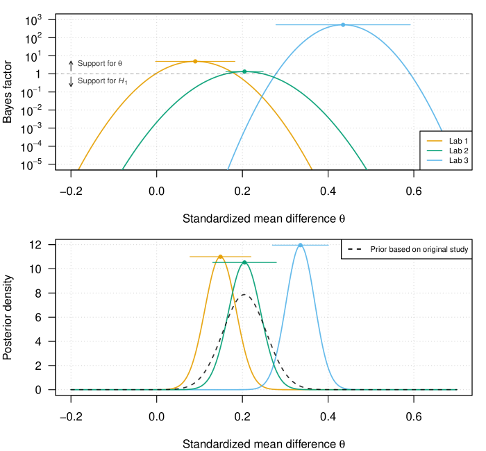
Figure 6: Bayes factor functions with maximum evidence estimates and $k=1$ support intervals (top) and posterior distribution with posterior modes and 95% highest posterior density credible intervals (bottom) for the three replication studies from the “Labels” experiment (Protzko et al., , 2023). The original study found an estimated standardized mean difference of $y_{o}=0.205$ with standard error $\sigma_{o}=0.051$ which is used to formulate the prior distribution under the alternative $\theta\mid H_{1}\sim\operatorname{N}(y_{o},\sigma^{2}_{o})$. The replication effect estimates were $y_{ri}\in\{0.09,0.205,0.435\}$ with standard errors $\sigma_{ri}\in\{0.052,0.057,0.044\}$, respectively, and are assumed to be normally distributed $y_{ri}\mid\theta\sim\operatorname{N}(\theta,\sigma^{2}_{ri})$. The posterior is obtained by multiplying the BFF with the prior density.

The top plot in Figure 6 shows the associated BFFs, MEEs, and $k=1$ support intervals. We see that, the BFFs peak at the corresponding replication estimate, but the height of these peaks differs between replications. The replication from lab 2 produced an effect estimate identical to the original one, so there is little support of its MEE over the alternative based on the original study as the estimates from both studies are in close agreement. In contrast, the MEEs from lab 1 and lab 3 receive substantial and very strong support over the alternative because they are either smaller or larger. In turn, their $k=1$ support intervals are much wider compared to the narrow support interval from lab 2. Finally, we can also see that the BFF from lab 1 indicates that there is absence of evidence regarding whether or not the data support the value of no effect ($\operatorname{BF}_{01}\approx 1$ at $\theta=0$), whereas the BFFs from labs 2 and 3 indicate strong and decisive evidence against no effect up to very small effects of around $\theta=0.1$, respectively.

The bottom plot in Figure 6 illustrates the posterior distributions, conveniently obtained by multiplying the BFF by the prior distribution based on the original data since this BFF has a Savage-Dickey density ratio representation. We can see that the $k=1$ support intervals from the top plot are given by the set of effect sizes with posterior density larger than the prior density. These posteriors represent a synthesis of the original and replication studies, as they lie somewhere in between the likelihood of the replication data and the prior based on the original study. For example, the posterior from lab 3 is centered around $0.34$ with 95% credible interval from $0.27$ to $0.4$. Clearly, this interval excludes both the original ($y_{o}=0.205$) and the replication effect estimates ($y_{r3}=0.435$), leading to a different conclusion from the BFF, which indicates decisive evidence for the MEE at $y_{r3}=0.435$ ($k_{\mathrm{ME}}=521$).

4.4 Logistic regression

To illustrate a computationally more involved application of BFFs, we consider the epidemiological study from Neutra et al., (1978), previously reanalyzed by Greenland, (2007) and Sullivan and Greenland, (2013). This study investigated the association between neonatal death and 14 exposure variables. Among the 2992 recorded births only 17 neonatal deaths occurred. This leads to challenges in conducting inferences with so many exposure variables, as we will see in the following.

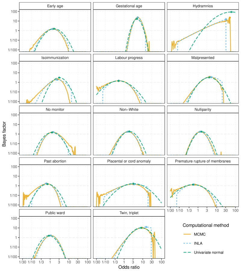
Figure 7: Multiple logistic regression BFF analysis of 2992 births with 17 neonatal deaths from Neutra et al., (1978) as reanalyzed by Sullivan and Greenland, (2013). Each plot shows the BFF related to the exponentiated regression coefficient which can be interpreted as odds ratio. Independent, weakly informative $\operatorname{N}(0,1/2)$ priors are assigned to the coefficients under the alternative $H_{1}$. All other coefficients were considered as nuisance parameters and the same priors assigned to them as under the alternative. Variables are binary indicators, except early age (0, 20 ,1 15 19, 2 under 15), gestational age ($0=\text{no}$, $1=36-38$ weeks, $2=33-36$ weeks; under 33 weeks excluded), isoimmunization ($0=\text{no}$, $1=\text{Rh}$, $2=\text{ABO}$), labour progress ($0=\text{no}$, $0.33=\text{prolonged}$, $0.67=\text{protracted}$, $1=\text{arrested}$) and past abortion ($0=\text{none}$, $1=1$, $2=2+$).

Figure 7 shows the BFFs related to a logistic regression analysis of the data including all exposures as main effects and an intercept term. Each BFF relates to the exponentiated regression coefficient, which can be interpreted as the multiplicative change of odds of neonatal death when increasing the variable by one unit while keeping all other variables fixed. An improper flat prior was assigned to the intercept under both the null and the alternative, while independent $\operatorname{N}(0,1/2)$ priors were assigned to the coefficients under the alternative. This prior represents an alternative postulating that the median odds ratio is $1$ and that $95\%$ of odds ratios are in between $1/4$ and $4$, representing a plausible range of odds ratios in epidemiology (Greenland, , 2006). For the analysis of each coefficient, all other coefficients were considered as nuisance parameters with the same priors assigned to them under the null as under the alternative.

BFFs were computed in three ways: i) By first computing the marginal posterior distribution for each coefficient from kernel smoothing of $10^{\prime}000^{\prime}000$ Markov chain Monte Carlo (MCMC) samples (solid orange lines) computed with Stan (Carpenter et al., , 2017) and then computing the BFF via the Savage-Dickey density ratio as explained in Section 3.4. ii) By computing the marginal posterior with integrated nested Laplace approximation (short-dashed blue lines) via INLA (Rue et al., , 2009) and then computing the BFF via the Savage-Dickey density. iii) By estimating the parameters of the logistic model first with maximum likelihood, and then using each estimated coefficient and its standard error for a univariate normal analysis as explained in Section 2.3, ignoring the nuisance parameters (long-dashed green lines). As a result, the MEEs from the univariate normal analysis correspond to maximum likelihood estimates, while the MEEs from the MCMC and INLA analyses correspond to integrated maximum likelihood estimates.

The MCMC analysis took the longest of the three (around 30 minutes to run), followed by the INLA analysis (about a second to run), followed by the univariate analysis (almost instantaneous). We can see that the BFFs based on MCMC and INLA (with default settings) may have inaccuracies or cannot be computed in the outer regions of the BFF, since these are regions where the posterior density is close to zero. We can also see that the univariate normal BFF agrees reasonably well with the MCMC and INLA BFFs in most cases, with the exception of the ’Hydramnios’ variable. In this case, the MCMC and INLA BFFs increase monotonically but end abruptly around OR = 50 and OR = 30, respectively, because no larger MCMC samples were observed or because the INLA algorithm returned a posterior density of zero. However, the shapes of the BFFs suggest that their maxima lie outside the range shown, and may even be larger than the maximum of the univariate normal BFF. Because of these computational issues, the ‘Hydramnios’ BFF should be interpreted with caution.

Due to the sparse nature of the data, most of the BFFs are undiagnostic about whether or not the variables exhibit harmful or beneficial associations with neonatal death. For example, the BFF (based on MCMC) for the variable ‘Early age’ (top left panel) has its mode at $\widehat{\text{OR}}_{\mathrm{ME}}=1.4$ indicating a slightly harmful association between early age pregnancy and neonatal death, yet this parameter value receives only anecdotal support over the alternative ($k_{\mathrm{ME}}=1.5$) and the corresponding $k=1$ support interval spans the range from beneficial ($\text{OR}=1/1.4$) up to harmful associations ($\text{OR}=2.5$).

For most variables, the BFFs indicate that strongly harmful ($\text{OR}>10$) associations are disfavoured by the data relative to the alternative. However, the variables ‘Gestational age’, ‘Hydramnios’, ‘Malpresented’, and ‘Twin, triplet‘ are notable exceptions. In each case, the BFFs suggest small up to very harmful associations with neonatal death. For example, for the variable ‘Hydramnios’ an MEE (based on univariate normal analysis) of $\widehat{\text{OR}}_{\mathrm{ME}}=60.3$ ($k=1$ support interval from $1.7$ to $2188$) is obtained. This extreme inflation reflects the fact that only one death was observed with hydramnios during pregnancy. The example illustrates that just as non-Bayesian methods, BFFs, support intervals, and MEEs can suffer from small-data artifacts. These could be avoided with a posterior distribution based on a weakly informative prior that shrinks the posterior toward more realistic values (Greenland, , 2006), with the caveat that a poorly chosen prior may also mask genuine signals from the data.

5 Discussion

We showed how Bayes factors can be used for parameter estimation, extending their traditional use cases of hypothesis testing and model comparison. We also linked these ideas to the overarching concept of Bayes factor functions (BFFs), which are Bayes factor analogues of P-value functions, and are likewise particularly useful for reporting of analysis results. This provides data analysts with a unified framework for statistical inference that is distinct from conventional frequentist and Bayesian approaches: While a P-value function can only quantify evidence against parameter values (Greenland, , 2023), BFFs allow us to quantify evidence in favour of parameter values over the alternative. Moreover, if a BFF diagnoses absence of evidence, data analysts can continue to collect data without worrying about multiplicity issues. Like ordinary Bayesian inference, BFF inference uses the Bayesian evidence calculus, but without synthesizing data and prior. When point priors are assigned, Bayes factors become likelihood ratios, so BFF inference aligns with likelihoodist inference, but when there are nuisance parameters, BFFs include a natural way to eliminate them via marginalization over a prior.

Like the likelihoodist and Neyman-Pearson paradigms of statistical inference, BFF inference requires the formulation of alternative hypotheses. For this reason, BFFs are particularly valuable in contexts where prior data or theories are available to formulate alternative hypotheses. For example, BFFs (under the name of ‘K ratio‘) have been used by the large-scale NANOGrav collaboration to quantify the evidence for new physics theories against the established Standard Model (Afzal et al., , 2023). In cases where there are no clear alternative hypotheses, data analysts may use BFFs based on ‘weakly informative‘ (Gelman, , 2009) or ‘default‘ prior distributions (e.g., unit-information priors, see Kass and Wasserman, , 1995), but should acknowledge this limitation and report sensitivity analyses (e.g., BFFs for different prior distributions). Another possibility is to base BFF inference on Bayes factor bounds (Berger and Sellke, , 1987; Sellke et al., , 2001; Held and Ott, , 2018), which give a bound on the maximum evidence against parameter values, but at the cost of losing the ability to quantify evidence in favour of parameter values (Pawel et al., , 2024).

Where under their control, data analysts should design experiments and studies so that conclusive inferences can be drawn from the data collected, including BFF inferences. Future research needs to investigate how experiments need to be designed to enable conclusive inference with BFFs. For example, one may design an experiment so that the expected width of a support interval is sufficiently narrow, or so that the expected evidence level for the MEE is sufficiently large. Finally, calculating BFFs can be challenging, as our logistic regression example showed. For example, if a BFF is computed via the Savage-Dickey density ratio from a posterior distribution computed by MCMC, the BFF may be imprecise at the tails of the posterior, even with millions of samples. Future work may focus on developing more efficient techniques for computing BFFs in such settings.

Bayesian, likelihoodist, or predictive reasoning may all motivate the Bayes factor as a natural tool for quantifying the relative evidence or support of competing hypotheses. Nevertheless, neither the Bayes factor nor any other measure of statistical evidence is infallible or suitable for all purposes. For example, Bayes factors by construction do not take into account the prior probabilities of their contrasted hypotheses, so they may indicate strong support for a hypothesis even though this hypothesis would still remain unlikely when combined with its prior probability (Lavine and Schervish, , 1999; Good, , 2001). Any type of statistical inference can lead to distorted scientific inferences if used in a bright-line fashion without consideration of contextual factors (Goodman, , 2016; Greenland, , 2023). We believe that BFFs are useful in this regard because they shift the focus from finding evidence against a single null hypothesis to making gradual and quantitative inferences.

Conflict of interest

We declare no conflict of interest.

Software and data

The data from Neutra et al., (1978) where obtained from the ‘fm0.asc’ file contained in ‘Supplementary Data.zip’ available at https://doi.org/10.1093/ije/dys213. The data from Bartoš et al., (2023) were obtained from the dat.bartos2023 data set included in the metadat R package (White et al., , 2023). The code and data to reproduce our analyses is openly available at https://github.com/SamCH93/BFF. A snapshot of the repository at the time of writing is available at https://doi.org/10.5281/zenodo.10817311. We used the statistical programming language R version 4.3.3 (2024-02-29) for analyses (R Core Team, , 2023) along with the brms (Bürkner, , 2021) and INLA (Rue et al., , 2009) packages for the computation of posterior distributions.

References

- Afzal et al., (2023) Afzal, A., Agazie, G., Anumarlapudi, A., Archibald, A. M., Arzoumanian, Z., Baker, P. T., Bécsy, B., Blanco-Pillado, J. J., Blecha, L., Boddy, K. K., Brazier, A., Brook, P. R., Burke-Spolaor, S., et al. (2023). The NANOGrav 15 yr data set: Search for signals from new physics. The Astrophysical Journal Letters, 951(1):L11. doi:10.3847/2041-8213/acdc91.
- Barnard, (1949) Barnard, G. A. (1949). Statistical inference. Journal of the Royal Statistical Society: Series B (Methodological), 11(2):115–139. doi:10.1111/j.2517-6161.1949.tb00028.x.
- Bartoš et al., (2023) Bartoš, F., Sarafoglou, A., Godmann, H. R., Sahrani, A., Leunk, D. K., Gui, P. Y., Voss, D., Ullah, K., Zoubek, M. J., Nippold, F., Aust, F., et al. (2023). Fair coins tend to land on the same side they started: Evidence from 350, 757 flips. doi:10.48550/ARXIV.2310.04153. arXiv preprint.
- Basu, (1977) Basu, D. (1977). On the elimination of nuisance parameters. Journal of the American Statistical Association, 72(358):355–366. doi:10.1080/01621459.1977.10481002.
- Bayarri et al., (2012) Bayarri, M. J., Berger, J. O., Forte, A., and García-Donato, G. (2012). Criteria for Bayesian model choice with application to variable selection. The Annals of Statistics, 40(3):1550–1577. doi:10.1214/12-aos1013.
- Bender et al., (2005) Bender, R., Berg, G., and Zeeb, H. (2005). Tutorial: Using confidence curves in medical research. Biometrical Journal, 47(2):237–247. doi:10.1002/bimj.200410104.
- Berger and Delampady, (1987) Berger, J. O. and Delampady, M. (1987). Testing precise hypotheses. Statistical Science, 2(3):317–335. doi:10.1214/ss/1177013238.
- Berger et al., (1999) Berger, J. O., Liseo, B., and Wolpert, R. L. (1999). Integrated likelihood methods for eliminating nuisance parameters. Statistical Science, 14(1). doi:10.1214/ss/1009211804.
- Berger and Sellke, (1987) Berger, J. O. and Sellke, T. (1987). Testing a point null hypothesis: The irreconcilability of values and evidence. Journal of the American Statistical Association, 82(397):112. doi:10.2307/2289131.
- Bernardo and Smith, (2000) Bernardo, J. M. and Smith, A. F. M. (2000). Bayesian Theory. John Wiley & Sons, Hoboken. doi:10.1002/9780470316870.
- Birnbaum, (1961) Birnbaum, A. (1961). Confidence curves: An omnibus technique for estimation and testing statistical hypotheses. Journal of the American Statistical Association, 56(294):246–249. doi:10.1080/01621459.1961.10482107.
- Blume, (2002) Blume, J. D. (2002). Likelihood methods for measuring statistical evidence. Statistics in Medicine, 21(17):2563–2599. doi:10.1002/sim.1216.
- Bürkner, (2021) Bürkner, P.-C. (2021). Bayesian item response modeling in R with brms and Stan. Journal of Statistical Software, 100(5):1–54. doi:10.18637/jss.v100.i05.
- Campbell and Gustafson, (2022) Campbell, H. and Gustafson, P. (2022). Bayes factors and posterior estimation: Two sides of the very same coin. The American Statistician, 77(3):248–258. doi:10.1080/00031305.2022.2139293.
- Carpenter et al., (2017) Carpenter, B., Gelman, A., Hoffman, M. D., Lee, D., Goodrich, B., Betancourt, M., Brubaker, M., Guo, J., Li, P., and Riddell, A. (2017). Stan: A probabilistic programming language. Journal of Statistical Software, 76(1). doi:10.18637/jss.v076.i01.
- Consonni et al., (2018) Consonni, G., Fouskakis, D., Liseo, B., and Ntzoufras, I. (2018). Prior distributions for objective Bayesian analysis. Bayesian Analysis, 13(2):627–679. doi:10.1214/18-ba1103.
- Cox, (1958) Cox, D. R. (1958). Some problems connected with statistical inference. The Annals of Mathematical Statistics, 29(2):357–372. doi:10.1214/aoms/1177706618.
- Dawid, (2011) Dawid, P. A. (2011). Posterior model probabilities. In Bandyopadhyay, P. S. and Forster, M. R., editors, Philosophy of Statistics, volume 7 of Handbook of the Philosophy of Science, pages 607–630. North-Holland, Amsterdam.
- Diaconis et al., (2007) Diaconis, P., Holmes, S., and Montgomery, R. (2007). Dynamical bias in the coin toss. SIAM Review, 49(2):211–235. doi:10.1137/s0036144504446436.
- Dickey, (1971) Dickey, J. M. (1971). The weighted likelihood ratio, linear hypotheses on normal location parameters. The Annals of Mathematical Statistics, 42(1):204–223. doi:10.1214/aoms/1177693507.
- Edwards, (1971) Edwards, A. W. F. (1971). Likelihood. Cambridge University Press, London.
- Evans, (1997) Evans, M. (1997). Bayesian inference procedures derived via the concept of relative surprise. Communications in Statistics - Theory and Methods, 26(5):1125–1143. doi:10.1080/03610929708831972.
- Evans, (2015) Evans, M. (2015). Measuring statistical evidence using relative belief. CRC Press, Boca Raton.
- Fowlie, (2024) Fowlie, A. (2024). The Bayes factor surface for searches for new physics. doi:10.48550/ARXIV.2401.11710. arXiv preprint.
- Franck and Gramacy, (2019) Franck, C. T. and Gramacy, R. B. (2019). Assessing Bayes factor surfaces using interactive visualization and computer surrogate modeling. The American Statistician, 74(4):359–369. doi:10.1080/00031305.2019.1671219.
- Fraser, (2019) Fraser, D. A. S. (2019). The p-value function and statistical inference. The American Statistician, 73(sup1):135–147. doi:10.1080/00031305.2018.1556735.
- Gelfand and Dey, (1994) Gelfand, A. E. and Dey, D. K. (1994). Bayesian model choice: Asymptotics and exact calculations. Journal of the Royal Statistical Society: Series B (Methodological), 56(3):501–514. doi:10.1111/j.2517-6161.1994.tb01996.x.
- Gelman, (2009) Gelman, A. (2009). Bayes, Jeffreys, prior distributions and the philosophy of statistics. Statistical Science, 24(2):176–178. doi:10.1214/09-sts284d.
- Gneiting and Raftery, (2007) Gneiting, T. and Raftery, A. E. (2007). Strictly proper scoring rules, prediction, and estimation. Journal of the American Statistical Association, 102(477):359–378. doi:10.1198/016214506000001437.
- Good, (1950) Good, I. J. (1950). Probability and the Weighing of Evidence. Griffin, London.
- Good, (1952) Good, I. J. (1952). Rational decisions. Journal of the Royal Statistical Society: Series B (Methodological), 14(1):107–114. doi:10.1111/j.2517-6161.1952.tb00104.x.
- Good, (1958) Good, I. J. (1958). Significance tests in parallel and in series. Journal of the American Statistical Association, 53(284):799–813. doi:10.1080/01621459.1958.10501480.
- Good, (2001) Good, I. J. (2001). Lavine, M., and Schervish, M. J. (1999), “Bayes factors: What they are and what they are not,” The American Statistician, 53, 119–122: Comment by Good and reply. The American Statistician, 55(2):171–174. doi:10.1198/000313001750358680.
- Goodman, (1999) Goodman, S. N. (1999). Toward evidence-based medical statistics. 2: The Bayes factor. Annals of Internal Medicine, 130(12):1005. doi:10.7326/0003-4819-130-12-199906150-00019.
- Goodman, (2016) Goodman, S. N. (2016). Aligning statistical and scientific reasoning. Science, 352(6290):1180–1181. doi:10.1126/science.aaf5406.
- Greenland, (2006) Greenland, S. (2006). Bayesian perspectives for epidemiological research: I. foundations and basic methods. International Journal of Epidemiology, 35(3):765–775. doi:10.1093/ije/dyi312.
- Greenland, (2007) Greenland, S. (2007). Bayesian perspectives for epidemiological research. ii. regression analysis. International Journal of Epidemiology, 36(1):195–202. doi:10.1093/ije/dyl289.
- Greenland, (2017) Greenland, S. (2017). Invited commentary: The need for cognitive science in methodology. American Journal of Epidemiology, 186(6):639–645. doi:10.1093/aje/kwx259.
- Greenland, (2023) Greenland, S. (2023). Divergence versus decision P‐values: A distinction worth making in theory and keeping in practice: Or, how divergence P‐values measure evidence even when decision P‐values do not. Scandinavian Journal of Statistics, 50(1):54–88. doi:10.1111/sjos.12625.
- Greenland et al., (2016) Greenland, S., Senn, S. J., Rothman, K. J., Carlin, J. B., Poole, C., Goodman, S. N., and Altman, D. G. (2016). Statistical tests, P values, confidence intervals, and power: a guide to misinterpretations. European Journal of Epidemiology, 31(4):337–350. doi:10.1007/s10654-016-0149-3.
- Grünwald et al., (2024) Grünwald, P., de Heide, R., and Koolen, W. (2024). Safe testing. Journal of the Royal Statistical Society Series B: Statistical Methodology. doi:10.1093/jrsssb/qkae011.
- Harms, (2019) Harms, C. (2019). A Bayes factor for replications of ANOVA results. The American Statistician, 73(4):327–339. doi:10.1080/00031305.2018.1518787.
- Harville, (1974) Harville, D. A. (1974). Bayesian inference for variance components using only error contrasts. Biometrika, 61(2):383–385. doi:10.1093/biomet/61.2.383.
- Held et al., (2022) Held, L., Matthews, R., Ott, M., and Pawel, S. (2022). Reverse-Bayes methods for evidence assessment and research synthesis. Research Synthesis Methods, 13(3):295–314. doi:10.1002/jrsm.1538.
- Held and Ott, (2018) Held, L. and Ott, M. (2018). On -values and Bayes factors. Annual Review of Statistics and Its Application, 5(1):393–419. doi:10.1146/annurev-statistics-031017-100307.
- Hendriksen et al., (2021) Hendriksen, A., de Heide, R., and Grünwald, P. (2021). Optional stopping with Bayes factors: A categorization and extension of folklore results, with an application to invariant situations. Bayesian Analysis, 16(3):961–989. doi:10.1214/20-ba1234.
- Hoeting et al., (1999) Hoeting, J. A., Madigan, D., Raftery, A. E., and Volinsky, C. T. (1999). Bayesian model averaging: a tutorial. Statistical Science, 14(4). doi:10.1214/ss/1009212519.
- Infanger and Schmidt-Trucksäss, (2019) Infanger, D. and Schmidt-Trucksäss, A. (2019). P value functions: An underused method to present research results and to promote quantitative reasoning. Statistics in Medicine, 38(21):4189–4197. doi:10.1002/sim.8293.
- Jeffreys, (1939) Jeffreys, H. (1939). Theory of Probability. Clarendon Press, Oxford, first edition.
- Jeffreys, (1961) Jeffreys, H. (1961). Theory of Probability. Clarendon Press, Oxford, third edition.
- Johnson et al., (2023) Johnson, V. E., Pramanik, S., and Shudde, R. (2023). Bayes factor functions for reporting outcomes of hypothesis tests. Proceedings of the National Academy of Sciences, 120(8). doi:10.1073/pnas.2217331120.
- Kalbfleisch and Sprott, (1970) Kalbfleisch, J. D. and Sprott, D. A. (1970). Application of likelihood methods to models involving large numbers of parameters. Journal of the Royal Statistical Society: Series B (Methodological), 32(2):175–194. doi:10.1111/j.2517-6161.1970.tb00830.x.
- Kass and Raftery, (1995) Kass, R. E. and Raftery, A. E. (1995). Bayes factors. Journal of the American Statistical Association, 90(430):773–795. doi:10.1080/01621459.1995.10476572.
- Kass and Vaidyanathan, (1992) Kass, R. E. and Vaidyanathan, S. K. (1992). Approximate Bayes factors and orthogonal parameters, with application to testing equality of two binomial proportions. Journal of the Royal Statistical Society: Series B (Methodological), 54(1):129–144. doi:10.1111/j.2517-6161.1992.tb01868.x.
- Kass and Wasserman, (1995) Kass, R. E. and Wasserman, L. (1995). A reference Bayesian test for nested hypotheses and its relationship to the Schwarz criterion. Journal of the American Statistical Association, 90(431):928–934. doi:10.1080/01621459.1995.10476592.
- Kerridge, (1963) Kerridge, D. (1963). Bounds for the frequency of misleading Bayes inferences. The Annals of Mathematical Statistics, 34(3):1109–1110. doi:10.1214/aoms/1177704038.
- Laird and Ware, (1982) Laird, N. M. and Ware, J. H. (1982). Random-effects models for longitudinal data. Biometrics, 38(4):963–974. doi:10.2307/2529876.
- Lavine and Schervish, (1999) Lavine, M. and Schervish, M. J. (1999). Bayes factors: What they are and what they are not. The American Statistician, 53(2):119–122. doi:10.1080/00031305.1999.10474443.
- Ly et al., (2018) Ly, A., Etz, A., Marsman, M., and Wagenmakers, E.-J. (2018). Replication Bayes factors from evidence updating. Behavior Research Methods, 51(6):2498–2508. doi:10.3758/s13428-018-1092-x.
- Marschner, (2024) Marschner, I. C. (2024). Confidence distributions for treatment effects in clinical trials: Posteriors without priors. Statistics in Medicine, 43(6):1271–1289. doi:10.1002/sim.10000.
- National Academies of Sciences, Engineering, and Medicine, (2019) National Academies of Sciences, Engineering, and Medicine (2019). Reproducibility and Replicability in Science. National Academies Press. doi:10.17226/25303.
- Neutra et al., (1978) Neutra, R. R., Fienberg, S. E., Greenland, S., and Friedman, E. A. (1978). Effect of fetal monitoring on neonatal death rates. New England Journal of Medicine, 299(7):324–326. doi:10.1056/nejm197808172990702.
- O’Hagan, (2019) O’Hagan, A. (2019). Expert knowledge elicitation: Subjective but scientific. The American Statistician, 73(sup1):69–81. doi:10.1080/00031305.2018.1518265.
- O’Hagan and Forster, (2004) O’Hagan, A. and Forster, J. (2004). Kendall’s Advanced Theory of Statistic 2B. Wiley & Sons, Chichester, second edition.
- Pawel et al., (2023) Pawel, S., Aust, F., Held, L., and Wagenmakers, E.-J. (2023). Power priors for replication studies. TEST. doi:10.1007/s11749-023-00888-5.
- Pawel and Held, (2022) Pawel, S. and Held, L. (2022). The sceptical Bayes factor for the assessment of replication success. Journal of the Royal Statistical Society: Series B (Statistical Methodology), 84(3):879–911. doi:10.1111/rssb.12491.
- Pawel et al., (2024) Pawel, S., Ly, A., and Wagenmakers, E.-J. (2024). Evidential calibration of confidence intervals. The American Statistician, 78(1):1–11. doi:10.1080/00031305.2023.2216239.
- Protzko et al., (2023) Protzko, J., Krosnick, J., Nelson, L., Nosek, B. A., Axt, J., Berent, M., Buttrick, N., DeBell, M., Ebersole, C. R., Lundmark, S., MacInnis, B., O’Donnell, M., Perfecto, H., Pustejovsky, J. E., Roeder, S. S., Walleczek, J., and Schooler, J. W. (2023). High replicability of newly discovered social-behavioural findings is achievable. Nature Human Behaviour. doi:10.1038/s41562-023-01749-9.
- R Core Team, (2023) R Core Team (2023). R: A Language and Environment for Statistical Computing. R Foundation for Statistical Computing, Vienna, Austria. URL https://www.R-project.org/.
- Rafi and Greenland, (2020) Rafi, Z. and Greenland, S. (2020). Semantic and cognitive tools to aid statistical science: replace confidence and significance by compatibility and surprise. BMC Medical Research Methodology, 20:244. doi:10.1186/s12874-020-01105-9.
- RECOVERY collaborative group, (2022) RECOVERY collaborative group (2022). Baricitinib in patients admitted to hospital with COVID-19 (RECOVERY): a randomised, controlled, open-label, platform trial and updated meta-analysis. The Lancet, 400(10349):359–368. doi:10.1016/s0140-6736(22)01109-6.
- Robbins, (1970) Robbins, H. (1970). Statistical methods related to the law of the iterated logarithm. The Annals of Mathematical Statistics, 41(5):1397–1409. doi:10.1214/aoms/1177696786.
- Rosenthal and Rubin, (1994) Rosenthal, R. and Rubin, D. B. (1994). The counternull value of an effect size: A new statistic. Psychological Science, 5(6):329–334. doi:10.1111/j.1467-9280.1994.tb00281.x.
- Röver et al., (2021) Röver, C., Bender, R., Dias, S., Schmid, C. H., Schmidli, H., Sturtz, S., Weber, S., and Friede, T. (2021). On weakly informative prior distributions for the heterogeneity parameter in Bayesian random-effects meta-analysis. Research Synthesis Methods, 12(4):448–474. doi:10.1002/jrsm.1475.
- Royall, (1997) Royall, R. (1997). Statistical Evidence: A likelihood paradigm. Chapman & Hall, London.
- Rue et al., (2009) Rue, H., Martino, S., and Chopin, N. (2009). Approximate Bayesian inference for latent Gaussian models by using integrated nested Laplace approximations. Journal of the Royal Statistical Society Series B: Statistical Methodology, 71(2):319–392. doi:10.1111/j.1467-9868.2008.00700.x.
- Schweder and Hjort, (2016) Schweder, T. and Hjort, N. L. (2016). Confidence, Likelihood, Probability. Cambridge University Press, Cambridge.
- Sellke et al., (2001) Sellke, T., Bayarri, M. J., and Berger, J. O. (2001). Calibration of values for testing precise null hypotheses. The American Statistician, 55(1):62–71. doi:10.1198/000313001300339950.
- Severini, (2007) Severini, T. A. (2007). Integrated likelihood functions for non-Bayesian inference. Biometrika, 94(3):529–542. doi:10.1093/biomet/asm040.
- Shalloway, (2014) Shalloway, D. (2014). The evidentiary credible region. Bayesian Analysis, 9(4):909–922. doi:10.1214/14-ba883.
- Stone, (1997) Stone, M. (1997). Discussion of papers by Dempster and Aitkin. Statistics and Computing, 7(4):263–264. doi:10.1023/a:1018502622516.
- Sullivan and Greenland, (2013) Sullivan, S. G. and Greenland, S. (2013). Bayesian regression in SAS software. International Journal of Epidemiology, 42(1):308–317. doi:10.1093/ije/dys213. erratum doi:10.1093/ije/dyu189.
- Verdinelli and Wasserman, (1995) Verdinelli, I. and Wasserman, L. (1995). Computing Bayes factors using a generalization of the Savage-Dickey density ratio. Journal of the American Statistical Association, 90(430):614–618. doi:10.1080/01621459.1995.10476554.
- Verhagen and Wagenmakers, (2014) Verhagen, J. and Wagenmakers, E.-J. (2014). Bayesian tests to quantify the result of a replication attempt. Journal of Experimental Psychology: General, 143(4):1457–1475. doi:10.1037/a0036731.
- Wagenmakers et al., (2022) Wagenmakers, E.-J., Gronau, Q. F., Dablander, F., and Etz, A. (2022). The support interval. Erkenntnis, 87(2):589–601. doi:10.1007/s10670-019-00209-z.
- Wagenmakers et al., (2010) Wagenmakers, E.-J., Lodewyckx, T., Kuriyal, H., and Grasman, R. (2010). Bayesian hypothesis testing for psychologists: A tutorial on the Savage–Dickey method. Cognitive Psychology, 60(3):158–189. doi:10.1016/j.cogpsych.2009.12.001.
- White et al., (2023) White, T., Noble, D., Senior, A., Hamilton, W. K., and Viechtbauer, W. (2023). metadat: Meta-Analysis Datasets. URL https://github.com/wviechtb/metadat. R package version 1.3-0.
- Xie and Singh, (2013) Xie, M. and Singh, K. (2013). Confidence distribution, the frequentist distribution estimator of a parameter: A review. International Statistical Review, 81(1):3–39. doi:10.1111/insr.12000.