A secular solar system resonance that disrupts the dominant cycle in Earth’s orbital eccentricity ($g_{2}$$-$$g_{5}$): Implications for astrochronology

Abstract

The planets’ gravitational interaction causes rhythmic changes in Earth’s orbital parameters (also called Milanković cycles), which have powerful applications in geology and astrochronology. For instance, the primary astronomical eccentricity cycle due to the secular frequency term ($g_{2}$$-$$g_{5}$) ($\sim$405 kyr in the recent past) utilized in deep-time analyses is dominated by Venus’ and Jupiter’s orbits, aka long eccentricity cycle. The widely accepted and long-held view is that ($g_{2}$$-$$g_{5}$) was practically stable in the past and may hence be used as a “metronome” to reconstruct accurate ages and chronologies. However, using state-of-the-art integrations of the solar system, we show here that ($g_{2}$$-$$g_{5}$) can become unstable over long time scales, without major changes in, or destabilization of, planetary orbits. The ($g_{2}$$-$$g_{5}$) disruption is due to the secular resonance $\mbox{$\sigma_{12}$}=(g_{1}-g_{2})+(s_{1}-s_{2})$, a major contributor to solar system chaos. We demonstrate that entering/exiting the $\sigma_{12}$ resonance is a common phenomenon on long time scales, occurring in $\sim$40% of our solutions. During $\sigma_{12}$-resonance episodes, ($g_{2}$$-$$g_{5}$) is very weak or absent and Earth’s orbital eccentricity and climate-forcing spectrum are unrecognizable compared to the recent past. Our results have fundamental implications for geology and astrochronology, as well as climate forcing because the paradigm that the longest Milanković cycle dominates Earth’s astronomical forcing, is stable, and has a period of $\sim$405 kyr requires revision.

1 Introduction

Laying the foundations of chaos theory, Henri Poincaré wrote: “It may happen that small differences in the initial conditions produce very great ones in the final phenomena. A small error in the former will produce an enormous error in the latter. Prediction becomes impossible $\ldots$” (Poincaré, 1914). In reference to the solar system, the sensitivity to initial conditions is indeed a key feature of the large-scale dynamical chaos in the system, which has been confirmed numerically (Sussman & Wisdom, 1988; Laskar, 1989; Ito & Tanikawa, 2002; Morbidelli, 2002; Varadi et al., 2003; Batygin & Laughlin, 2008; Zeebe, 2015; Brown & Rein, 2020; Abbot et al., 2023). Dynamical chaos affects the secular frequencies $g_{i}$ and $s_{i}$ (see Appendix A), where the terms ($g_{4}$$-$$g_{3}$) and ($s_{4}$$-$$s_{3}$), for instance, show chaotic behavior already on a 50-Myr time scale. As a result, astronomical solutions diverge around $t=\pm 50$ Myr, which fundamentally prevents identifying a unique solution on time scales $\stackrel{{\scriptstyle>}}{{\sim}}\$10⁸ y (Laskar et al., 2004; Zeebe, 2017; Zeebe & Lourens, 2019). The chaos therefore not only severely limits our understanding and ability to reconstruct and predict the solar system’s history and long-term future, it also imposes strict limits on geological and astrochronological applications such as developing a fully calibrated astronomical time scale beyond $\sim$50 Ma (for recent efforts, see Zeebe & Lourens, 2019, 2022). In contrast to these limitations (largely due to unstable terms such as ($g_{4}$$-$$g_{3}$) and ($s_{4}$$-$$s_{3}$)), another frequency term appears more promising as it shows more stable behavior. For example, it has hitherto been assumed that ($g_{2}$$-$$g_{5}$) was practically stable in the past and has been suggested for use as a “metronome” in deep-time geological applications, i.e., far exceeding 50 Ma (Laskar et al., 2004; Kent et al., 2018; Spalding et al., 2018; Meyers & Malinverno, 2018; Montenari, 2018; Lantink et al., 2019; De Vleeschouwer et al., 2024). The ($g_{2}$$-$$g_{5}$) cycle, which is the dominant term in Earth’s orbital eccentricity in the recent past ($\sim$405 kyr, see Fig. 1a) may thus have been regarded as an island of stability in a sea of chaos. However, we show in this contribution that also ($g_{2}$$-$$g_{5}$) can become unstable over long time scales.

Solar system dynamics affect Earth’s orbital evolution, as well as Earth’s climate, which is paced by astronomical cycles on time scales $\stackrel{{\scriptstyle>}}{{\sim}}\$10 kyr. The cycles include precession and obliquity cycles of Earth’s spin axis ($\sim$20 and 40 kyr in the recent past), and the short and long eccentricity cycles ($\sim$100 and 405 kyr, see Figs. 1a and 6) (Milanković, 1941; Montenari, 2018). Orbital eccentricity is controlled by the solar system’s orbital dynamics and is the focus of this study. The primary tuning target used in astrochronology and cyclostratigraphy for deep-time stratigraphic age models is the long eccentricity cycle (LEC) because it is widely assumed to be stable in the past (see above). Dynamically, Earth’s orbital eccentricity and inclination cycles originate from combinations of the solar system’s fundamental frequencies, called $g$- and $s$-frequencies (or modes), loosely related to the apsidal and nodal precession of the planetary orbits (Fig. A.1). The LEC is dominated by Venus’ and Jupiter’s orbits, viz., ($g_{2}-g_{5})$, or $g_{25}$ for short, and represents the strongest cycle in Earth’s eccentricity spectrum in the recent past (see Figs. 1 and 6). Assuming a stable LEC may appear plausible because Jupiter (dominating $g_{5}$) is the most massive planet and less susceptible to perturbations. Astronomical computations have confirmed $g_{5}$’s stability and hitherto did not indicate instabilities in $g_{25}$ (Berger, 1984; Quinn et al., 1991; Varadi et al., 2003; Laskar et al., 2004; Zeebe, 2017; Spalding et al., 2018; Zeebe & Lourens, 2022). However, compared to $g_{5}$, $g_{2}$’s long-term stability is less certain but has been overlooked so far. The long-term stability of $g_{25}$ and the LEC is critical for, e.g., climate forcing/insolation, constructing accurate age models and chronologies, expanding the evidence for the astronomical theory of climate into the more distant past, extending the astronomically calibrated geological time scale into deep time, and more (see discussion). Below we show that the LEC can become unstable over long-time scales owing to $g_{2}$, without major changes in, or destabilization of, planetary orbits. Orbital destabilization is a known, separate dynamical phenomenon relevant to the future, see below.

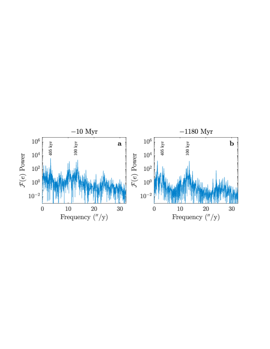
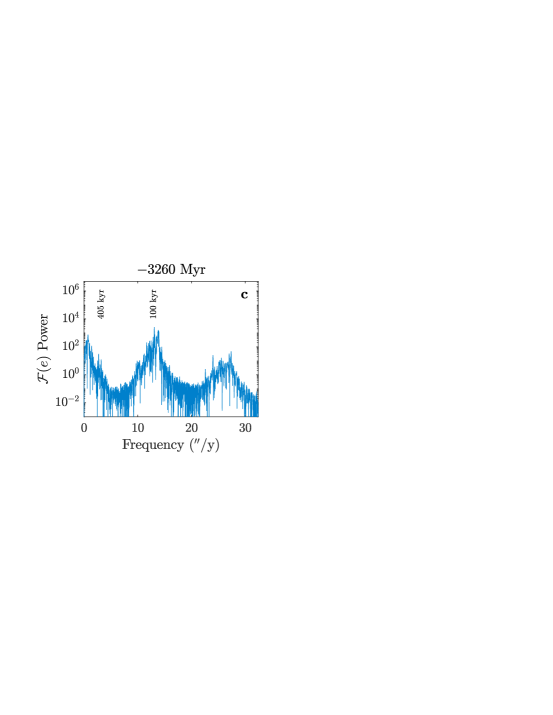
Figure 1: Fast Fourier transform (FFT $={\cal F}(e)$) over 20-Myr intervals of Earth’s orbital eccentricity. Frequencies in arcsec y^-1 = ” y^-1. (a) Standard spectrum in the recent past centered at $t=-10$ Myr (nearly identical in all solutions). Note the dominant ($g_{2}$$-$$g_{5}$) 405-kyr LEC. (b) and (c) Spectra of solutions R06 (Run 06) and R45 during $\sigma_{12}$-resonance episodes (see Section 3) centered at $t=-1180$ Myr and $t=-3260$ Myr, respectively. Note the unrecognizable spectrum pattern in (c) compared to (a) and the reduced/absence of power around the LEC frequency of $\sim$3.2” y^-1 ($\sim$405 kyr) in (b) and (c). The peaks around 10 to 13” y^-1 are due to the short eccentricity cycle.

For the present study, we performed state-of-the-art solar system integrations, including the eight planets and Pluto, a lunar contribution, general relativity, the solar quadrupole moment, and solar mass loss (see Section 2) (Zeebe, 2017; Zeebe & Lourens, 2019; Zeebe, 2022, 2023). Initial conditions at time $t_{0}$ were taken from the latest JPL ephemeris DE441 (Park et al., 2021) and the equations of motion were numerically integrated to $t=-3.5$ Gyr (beyond $-3.5$ Gyr parameters such as the lunar distance have large uncertainties, see Section 2). Owing to solar system chaos, the solutions diverge around $t=-50$ Myr, which prevents identifying a unique solution on time scales $\stackrel{{\scriptstyle>}}{{\sim}}\$10⁸ y (see above). Hence we present results from long-term ensemble integrations to explore the possible solution/phase space of the system (see Section 2). Importantly, because of the chaos, each $\sim$$10^{8}$ y interval of the integrations represents a snapshot of the system’s general/possible behavior that is largely independent of the actual numerical time of a particular solution (provided here that $t<-\mbox{$\tau_{12}$}$, where $\tau_{12}$ is of order $10^{8}$ to $10^{9}$ y, see below). In other words, a numerical solution’s behavior around, say, $t=-1.5$ Gyr may represent the actual solar system around $t=-600$ Myr and so on.

2 Methods

2.1 Solar System Integrations

Solar system integrations were performed following our earlier work (Zeebe, 2017; Zeebe & Lourens, 2019; Zeebe, 2022) with our integrator package orbitN (v1.0) (Zeebe, 2023), using a symplectic integrator and Jacobi coordinates (Wisdom & Holman, 1991; Zeebe, 2015a). The open source code is available at zenodo.org/records/8021040 and github.com/rezeebe/orbitN. The methods used here and our integrator package have been extensively tested and compared against other studies (Zeebe, 2017; Zeebe & Lourens, 2019; Zeebe, 2022, 2023). For the present study, we also included simulations with an independent integrator package (HNBody) (Rauch & Hamilton, 2002) and found the same dynamical behavior. All simulations include contributions from general relativity, available in orbitN as Post-Newtonian effects due to the dominant mass. The Earth-Moon system was modeled as a gravitational quadrupole (Quinn et al., 1991; Varadi et al., 2003; Zeebe, 2017, 2023). Initial conditions for the positions and velocities of the planets and Pluto were generated from the latest JPL ephemeris DE441 (Park et al., 2021) using the SPICE toolkit for Matlab. Coordinates were obtained at JD2451545.0 in the ECLIPJ2000 reference frame and subsequently rotated to account for the solar quadrupole moment ($J_{2}$) alignment with the solar rotation axis (Zeebe, 2017). Solar mass loss was included using $\dot{M}/M=-7\times 10^{-14}$ y^-1 (e.g., Quinn et al., 1991). As solar mass loss causes a secular drift in total energy, we added test runs with $M=const.$ to check the integrator’s numerical accuracy. Total energy and angular momentum errors were small throughout the 3.5-Gyr integrations (relative errors: $\stackrel{{\scriptstyle<}}{{\sim}}\$$6\times 10^{-10}$ and $\stackrel{{\scriptstyle<}}{{\sim}}\$$7\times 10^{-12}$, see Fig. 2). Our default numerical timestep ($|\Delta t|=4$ days) is close to the previously estimated value of 3.59 days to sufficiently resolve Mercury’s perihelion (Wisdom, 2015; Hernandez et al., 2022; Abbot et al., 2023). In additional eight simulations, we tested $|\Delta t|=2.15625$ days (adequate to $\mbox{$e_{\scriptsize\mercury}$}\ \raisebox{-2.15277pt}{$\stackrel{{\scriptstyle<}}{{\sim}}\ $}0.4$) and found no difference in terms of $\sigma_{12}$-resonances (see below), which occurred in 3/8 solutions.

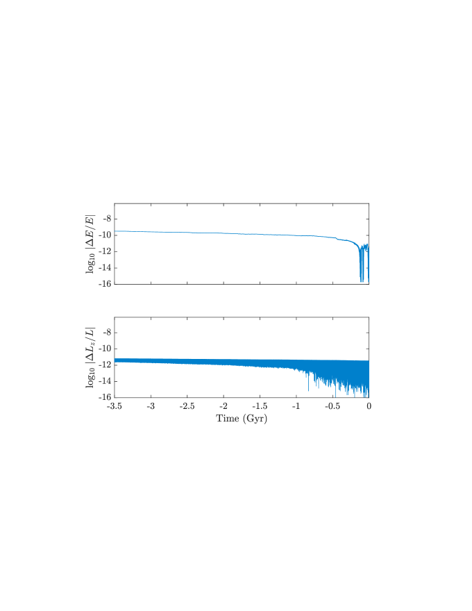
Figure 2: Relative errors in total energy ($E$) and angular momentum ($L_{z}$) of 3.5-Gyr test integrations (solar mass = $const.$). $|\Delta E/E|=|E(t)-E(0)/E(0)|$, $|\Delta L_{z}/L|=|L_{z}(t)-L_{z}(0)/L(0)|$. Due to $J_{2}$, only $L_{z}$ is conserved, not the horizontal components.

2.2 Ensemble Integrations

We performed ensemble integrations of the solar system with a total of $N=64$ members. Note that a larger $N$ is unnecessary for the current problem, which samples a common phenomenon ($\sim$40% of solutions), not a rare event, which requires large $N$ (Abbot et al., 2023). Different solutions were obtained by offsetting Earth’s initial position by a small distance (largest offset $\Delta x_{0}\simeq 1\times 10^{-12}$ au), which is within observational uncertainties (Zeebe, 2015, 2017). The different $\Delta x_{0}$ lead to complete randomization of solutions on a time scale of $\sim$50 Myr due to solar system chaos. We also tested different histories of the Earth-Moon distance ($R$), which has little effect on our results (see Section 2.3). Because of the large uncertainties in $R$ prior to $\sim$$3$ Ga, we restrict our integrations to $t=-3.5$ Gyr. Our solutions are available at www.ncdc.noaa.gov/paleo/study/xxxxx and www2.hawaii.edu/~zeebe/Astro.html.

2.3 Past Earth-Moon distance

Our integrations included a lunar contribution, i.e., a gravitational quadrupole model of the Earth-Moon system (Quinn et al., 1991; Varadi et al., 2003; Zeebe, 2017, 2023). In the present context, the lunar contribution has a relatively small effect on the overall dynamics, yet the integration requires the Earth-Moon distance ($R$) as parameter at a given time in the past. We tested two approaches, both avoiding the known problem of unrealistically small $R$ at $-3.5$ Gyr (see Fig. 3). ($i$) A linear extrapolation of $R$ into the past starting with $dR_{0}/dt$ close to the present rate and ($ii$) a 3rd-order polynomial fit to observations. The two approaches made essentially no difference in our computations and both yielded solutions including $\sigma_{12}$-resonance intervals at a similar frequency (see below). For the observational constraints on $R$, we selected robust data sets based on the reconstruction of Earth’s axial precession frequency obtained by cyclostratigraphic studies (Meyers & Malinverno, 2018; Lantink et al., 2022; Sørensen et al., 2020; De Vleeschouwer, D. $et~{}al$, 2023) (see Fig. 3). The classical integration of precession equations starting at the present rate $dR_{0}/dt$ (see Fig. 3, green dashed line) follows MacDonald (1964); Goldreich (1966); Touma & Wisdom (1994).

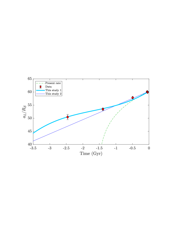
Figure 3: Past Earth-Moon distance ($R$) in units of Earth radii ($R_{E}$). Green dashed line: Integration of precession equations starting at present rate $dR_{0}/dt$ (see text), yielding (well-known) unrealistic past $R/R_{E}$. Red diamonds: Observational estimates based on robust data sets from cyclostratigraphic studies. Blue and cyan lines: Used in the present study. Blue: linear extrapolation into the past starting with $dR_{0}/dt$ close to the present rate. Cyan: 3rd-order polynomial fit to observations. Using $R/R_{E}$ based on the blue and cyan lines made essentially no difference in our computations; both approaches yielded solutions including $\sigma_{12}$-resonance intervals at a similar frequency (see Section 3).

2.4 Time series analysis of astronomical solutions

The solar system’s fundamental $g$- and $s$-frequencies were determined from the output of our numerical integrations using fast Fourier transform (FFT) over consecutive 20-Myr intervals. For the spectral analysis (see Figs. 4 and 5), we used Earth’s orbital elements and the classic variables:

$$h=e\sin(\varpi)\quad \quad k=e\cos(\varpi)$$ ; (1)

$$p=\sin(I/2)\ \sin\mbox{$\Omega$}\quad \quad q=\sin(I/2)\ \cos\mbox{$\Omega$}\ ,$$ ; (2)

where $e$, $I$, $\varpi$, and $\Omega$ are eccentricity, inclination, longitude of perihelion, and longitude of ascending node, respectively. The spectra for Earth’s $k$ and $q$, for example, show strong peaks at nearly all $g$- and $s$-frequencies, respectively (see Fig. 5). The $g$- and $s$-modes are loosely related to the apsidal and nodal precession of the planetary orbits (see Fig. A.1). However, there is generally no simple one-to-one relationship between a single mode and a single planet, particularly for the inner planets. The system’s motion is a superposition of all modes, although for the outer planets, some modes are dominated by a single planet.

2.5 Resonant angle

The resonant angle $\theta_{12}$ associated with the $\sigma_{12}$ resonance (see Eq. (6)) was determined following Lithwick & Wu (2011). The method is numerically efficient and easy to implement. Consider Eqs. (1) and (2), and use $\sin(I/2)\simeq I/2$ (applicable to small $I$, as in our solutions). The variable pairs $(h,k)$ and $2(p,q)$ can then be combined into two complex variables for each planet ($\hat{\imath}=\sqrt{-1}$):

$$z_{k} = e_{k}\exp(\hat{\imath}\ \varpi_{k})$$ (3)

$$\zeta_{k} = I_{k}\exp(\hat{\imath}\ \mbox{$\Omega$}_{k})\ ,$$ (4)

where index $k=M,V,E,\ldots,N$ refers to the planets. The $(z_{k},\zeta_{k})$ for $k=M,V$, for instance, were determined from Mercury’s and Venus’ computed orbital elements. Next, we applied a simple bandpass filter (rectangular window) centered on the fundamental frequencies $g_{i}$ and $s_{i}$ of interest (index $i$). For example, for $i=1,2$, the passed frequency range was set to $[g_{1}\ g_{2}]\pm 10\%$ and $[s_{1}\ s_{2}]^{+20\%}_{-10\%}$. The filtered (complex) quantities $(z^{*}_{i},\zeta^{*}_{i})$ then represent variables in which the magnitudes $|z^{*}_{i}|,|\zeta^{*}_{i}|$ are related to the planets, $|z^{*}_{i}|\simeq e_{k}$ and $|\zeta^{*}_{i}|\simeq I_{k}$ (see Fig. 9 and Lithwick & Wu (2011) for details). The phase angles $\varpi^{*}_{i}$ and $\mbox{$\Omega$}^{*}_{i}$ are related to the fundamental modes, $\varpi^{*}_{i}=\mbox{atan2}\{\Im(z^{*}_{i}),\Re(z^{*}_{i})\}$ and $\mbox{$\Omega$}^{*}_{i}=\mbox{atan2}\{\Im(\zeta^{*}_{i}),\Re(\zeta^{*}_{i})\}$, where $\Im$ and $\Re$ denote the imaginary and real part of a complex number. Finally, the resonant angle $\theta_{12}$ associated with $\sigma_{12}$ (see Eq. (6)) is calculated as:

$$\mbox{$\theta_{12}$}=(\varpi^{*}_{1}-\varpi^{*}_{2})+(\mbox{$\Omega$}^{*}_{1}-\mbox{$\Omega$}^{*}_{2})\ .$$ (5)

3 Results

3.1 Secular frequencies and eccentricity

Contrary to expectations, we found in $\sim$40% of the solutions that $g_{25}$ was not stable at a period $\mbox{$P_{25}$}\simeq 405$ kyr but shifted abruptly due to shifts in $g_{2}$ (Fig. 4). Importantly, in those cases the $g_{2}$ spectral peak usually split into two peaks at significantly reduced power (Fig. 5), resulting in a very weak or absent LEC (Fig. 6). Note that for, e.g., geological applications, the weak/absent LEC is crucial, not the actual value of the $P_{25}$ shift (Fig. B.1), which is immaterial because it would be unidentifiable in a stratigraphic record owing to the low $g_{25}$ power. Time series analysis of the solutions (see Section 2) revealed that the weak LEC intervals are associated with a secular resonance between the $g$- and $s$-modes dominated by Mercury and Venus ($|g_{1}-g_{2}|\simeq|s_{1}-s_{2}|$), dubbed $\sigma_{12}$:

$$\mbox{$\sigma_{12}$}=(g_{1}-g_{2})+(s_{1}-s_{2})\ .$$ (6)

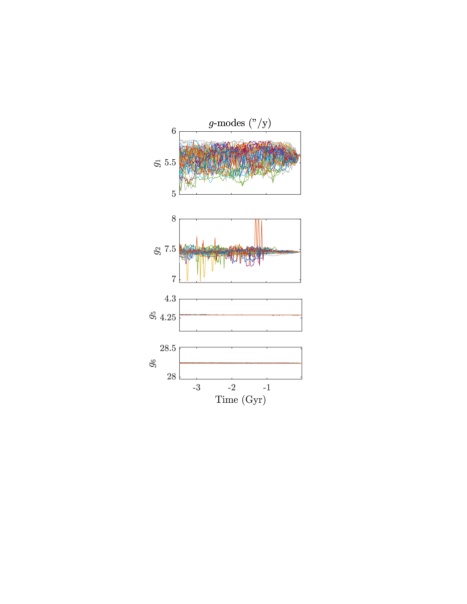
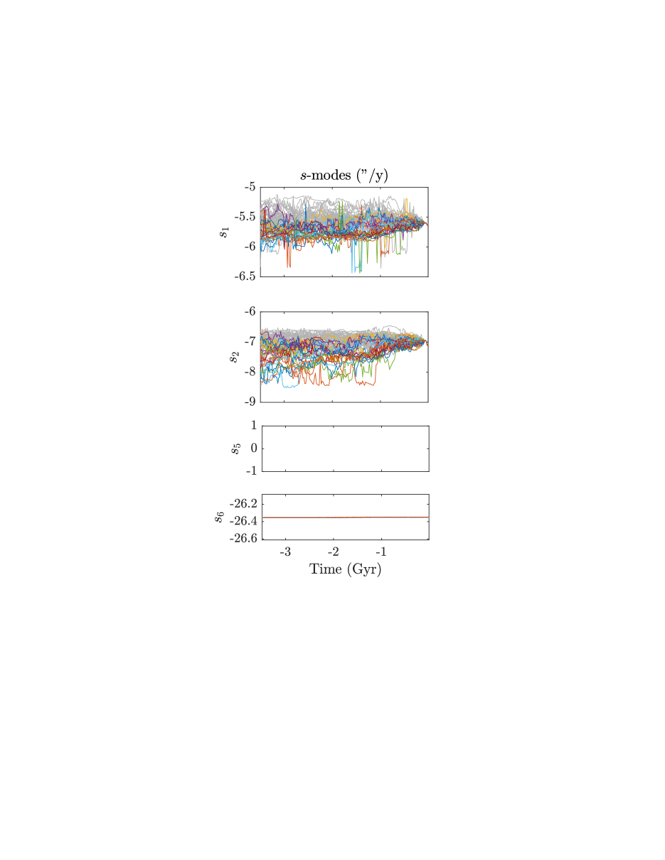
Figure 4: Evolution of fundamental solar system frequencies. The $g$- and $s$-frequencies (in arcsec y^-1 = ” y^-1) were determined from our solar system integrations using fast Fourier transform (FFT) over consecutive 20-Myr intervals and Earth’s $k$ and $q$ variables (see Section 2). The $g$- and $s$-modes are loosely related to the apsidal and nodal precession of the planetary orbits (see Fig. A.1). Solutions including $\sigma_{12}$-resonance intervals ($\sim$40%) are highlighted in color, the remaining solutions are displayed in gray. The frequencies $g_{1}$, $s_{1}$, and $s_{2}$ drift most strongly over time owing to chaotic diffusion. In addition, $g_{2}$ shows large and rapid shifts (spikes) at specific times when the spectral $g_{2}$ peak splits into two peaks at significantly reduced power during $\sigma_{12}$-resonance episodes (see Fig. 5). Alternating maximum power between the two peaks then causes the spikes in $g_{2}$. As a result, $\mbox{$g_{25}$}=(g_{2}-g_{5})$ is unstable and weak/absent during $\sigma_{12}$-resonance intervals (see Fig. B.1). $g_{5}$, $g_{6}$, and $s_{6}$ (dominated by Jupiter and Saturn) are practically stable over 3.5 Gyr ($s_{5}$ is zero due to conservation of total angular momentum/existence of an invariable plane, see Fig. A.1).

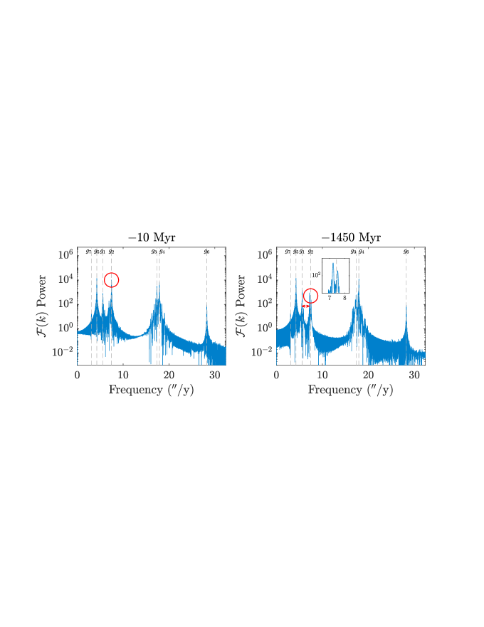
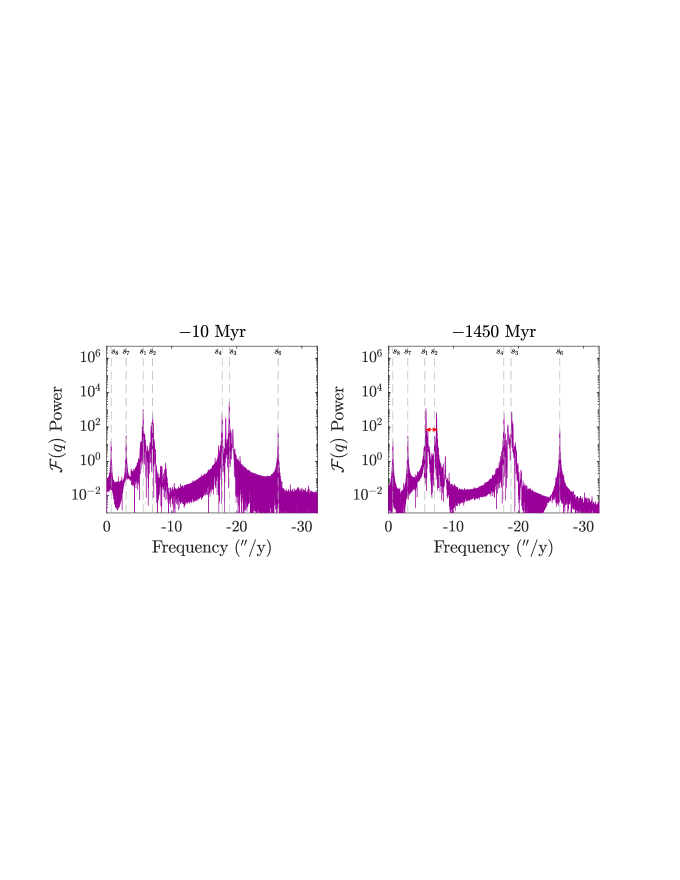
Figure 5: Time series analysis of astronomical solutions. Top and bottom: $g$- and $s$-spectra determined from our solar system integrations using fast Fourier transform (FFT $={\cal F}(k,q)$) over 20 Myr intervals and Earth’s $k$ and $q$ variables (see Section 2). Frequencies in arcsec y^-1 = ” y^-1. Left: Standard spectra in the recent past centered at $t=-10$ Myr (nearly identical in all solutions). Right: spectra of solution R28 centered at $t=-1450$ Myr (see Fig. 6b). The dashed lines indicate frequencies in the recent past (left) in all panels. During $\sigma_{12}$-resonance intervals (right), $g_{2}$ shows reduced power and generally splits into two peaks (red circles and inset). In the recent past (left), $|g_{2}-g_{1}|>|s_{2}-s_{1}|$, whereas during $\sigma_{12}$ resonances (right) $|g_{2}-g_{1}|\simeq|s_{2}-s_{1}|$ (see double arrows).

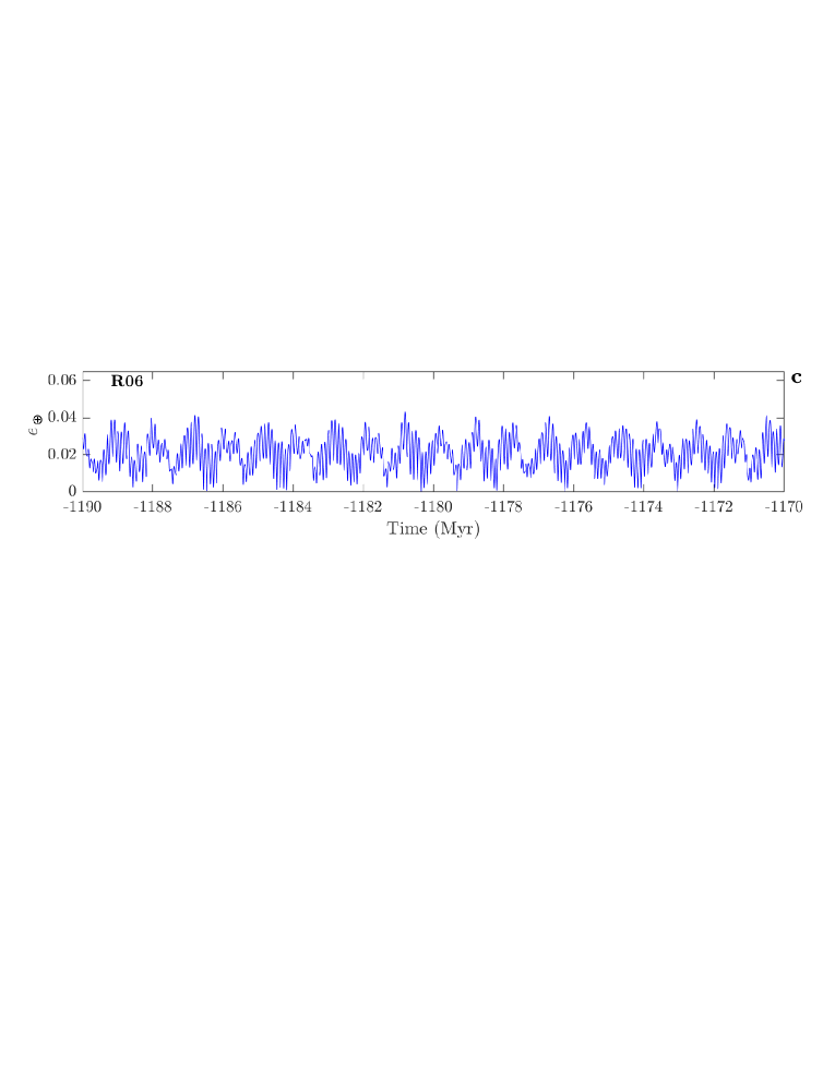
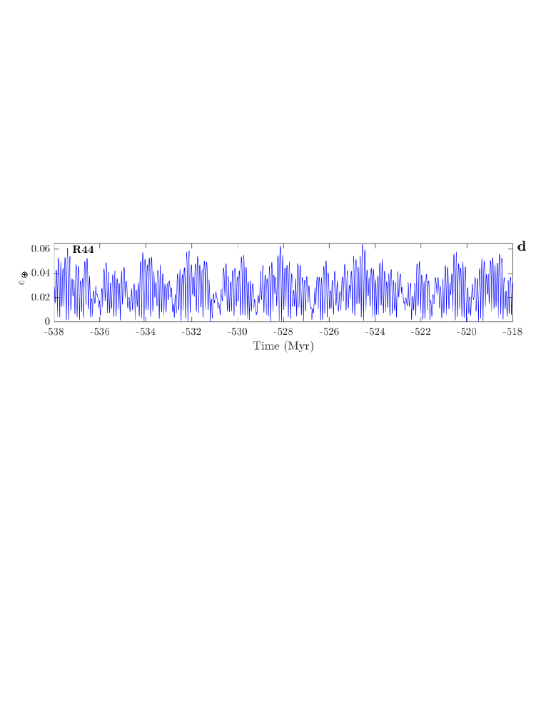
Figure 6: Earth’s orbital eccentricity from ensemble integrations. (a) Eccentricity pattern in the recent past (last 20 Myr) with short and long ($\sim$100 and $\sim$405 kyr) cycles (nearly identical in all solutions). Note the strong bundling of four short cycles into one long cycle (highlighted by 405 kyr filter). Panels (b, c, d) display examples of solutions during $\sigma_{12}$-resonance intervals. (b) Solution R28 (Run 28) over a 20-Myr interval centered at $t=-1450$ Myr. The LEC is virtually absent and the eccentricity pattern is unrecognizable compared to (a). (c) Solution R06 over a 20-Myr interval centered at $t=-1180$ Myr. In addition to a weak LEC, the maximum eccentricity is reduced to $\sim$0.04, which affects the total insolation Earth receives over one year (see text). (d) Solution R44 over a 20-Myr interval centered at $t=-528$ Myr; the LEC is present but weak relative to the short eccentricity cycle.

Several observations lend confidence to the robustness of our astronomical computations. ($i$) The methods used here and our integrator package have been extensively tested and compared against other studies (Zeebe, 2017; Zeebe & Lourens, 2019; Zeebe, 2022, 2023). ($ii$) The $\sigma_{12}$ resonance was recognized previously, although to our knowledge only by two studies (Lithwick & Wu, 2011; Mogavero & Laskar, 2022) and not its effect on $g_{25}$/LEC (see below). ($iii$) We tested an independent integrator package (HNBody Rauch & Hamilton (2002), see Section 2) and found the same dynamical behavior. ($iv$) Re-examination of previous 5-Gyr future integrations from this group (Zeebe, 2015) also revealed various solutions with $\sigma_{12}$-resonance intervals. ($v$) Total energy and angular momentum errors were small throughout our present 3.5-Gyr integrations (relative errors in test runs: $\stackrel{{\scriptstyle<}}{{\sim}}\$$6\times 10^{-10}$ and $\stackrel{{\scriptstyle<}}{{\sim}}\$$7\times 10^{-12}$, Fig. 2) and our numerical timestep sufficiently resolves Mercury’s perihelion (Wisdom, 2015; Hernandez et al., 2022; Abbot et al., 2023) (see Section 2).

During $\sigma_{12}$-resonance episodes, Earth’s orbital eccentricity pattern and hence Earth’s climate forcing spectrum due to eccentricity becomes unrecognizable compared to the recent past (Figs. 1 and 6). For example, a geologist examining a climate record exhibiting Milanković cycles within the $\sigma_{12}$ resonance (e.g., Fig. 6b-d) would fail to identify the rhythm as eccentricity cycles, given the currently known pattern (Fig. 6a). The resonance motifs are so different that (coincidentally) some frequency and amplitude modulation (AM) features (Fig. 6c) show more similarities with Mars’ orbital inclination in the recent past (Fig. C.1) (Zeebe, 2022) than Earth’s eccentricity (Fig. 6a). The estimated time scale $\tau_{12}$ for a possible $\sigma_{12}$-resonance occurrence ($\mbox{$\tau_{12}$}=$ temporal distance to the present) is of order $10^{8}$ to $10^{9}$ y. In several solutions, we found reduced $g_{2}$ and $g_{25}$ power (lower than short eccentricity power), as well as unusual eccentricity patterns, at $t\ \raisebox{-2.15277pt}{$\stackrel{{\scriptstyle<}}{{\sim}}\ $}-500$ Myr (see e.g., Fig. 6d) and in one solution at $t\simeq-420$ Myr. However, we have so far tested only 64 solutions (see Section 2), hence the youngest possible age of a $\sigma_{12}$-resonance interval that could be detectable in the geologic record is yet unknown. The duration of a $\sigma_{12}$-resonance episode may range from a few Myr to tens of millions of years (multiple entries/exits often occurring over several 100 Myr, see Figs. 6 and  9).

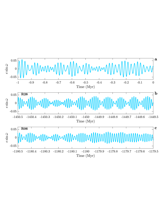
Figure 7: Climatic precession $\bar{p}=e\sin\bar{\omega}$, where $\bar{\omega}$ is the longitude of perihelion measured from the moving equinox (for details and code, see (Zeebe, 2022), github.com/rezeebe/snvec, www2.hawaii.edu/~zeebe/Astro.html, and Section 2.3. (a) $\bar{p}$ in the recent past (last 1 Myr), nearly identical in all solutions. Panels (b, c) display examples of $\bar{p}$ based on orbital solutions during $\sigma_{12}$-resonance intervals. Note the different lunisolar precession frequencies (carrier frequency) in the past owing to the Earth-Moon system’s evolution. (b) $\bar{p}$ based on solution R28 over a 1-Myr interval centered at $t=-1450$ Myr. The amplitude modulation (AM) pattern fundementally differs from (a). (c) $\bar{p}$ based on R06 over a 1-Myr interval centered at $t=-1180$ Myr. In addition to an altered AM pattern, the total amplitude is reduced compared to (a).

3.2 Insolation and climatic precession

The total mean annual insolation (or energy $W$) Earth’s receives is a function of its orbital eccentricity ($e_{\scriptsize\earth}$):

$$W\propto\left(1-\mbox{$e_{\scriptsize\earth}$}^{2}\right)^{-\frac{1}{2}}\ .$$ (7)

In the recent past, $0\ \raisebox{-2.15277pt}{$\stackrel{{\scriptstyle<}}{{\sim}}\ $}\mbox{$e_{\scriptsize\earth}$}\raisebox{-2.15277pt}{$\stackrel{{\scriptstyle<}}{{\sim}}\ $}0.06$, whereas during $\sigma_{12}$-resonance episodes, $\max\{\mbox{$e_{\scriptsize\earth}$}\}$ may be as low as $\sim$0.04 (Fig. 6c). Thus, the relative variation/difference in $W$ between eccentricity maxima and minima $((1-0^{2})^{-\frac{1}{2}}=1)$ is substantially reduced by the factor:

$$\left((1-0.06^{2})^{-\frac{1}{2}}-1\right)\ \left/\ \left((1-0.04^{2})^{-\frac{1}{2}}-1\right)\ \right.$$

$$=2.25\ .$$ (8)

Thus, in addition to a weak/absent LEC, both the total variation in eccentricity climate forcing and the extreme values are diminished on a $10^{6}$-year time scale during $\sigma_{12}$ intervals. Moreover, the $\sigma_{12}$ resonance causes major changes in climatic precession ($\bar{p}$), the primary climate driver on the shortest Milanković time scale ($\sim$20 kyr in the recent past). The main $\bar{p}$ frequencies are given by $\Psi+g_{i}$, where $\Psi$ is the lunisolar precession frequency. The disruption of $g_{2}$ (and hence $\Psi+g_{2}$) causes major changes in $\bar{p}$’s total amplitude and AM (see Figs. 7 and 8). For example, during $\sigma_{12}$-resonance intervals, the forcing power at the $\Psi+g_{2}$ precession frequency may drop by orders of magnitudes compared to the recent past (Fig. 8). The altered forcing in both, eccentricity and climatic precession, would scale down the climate response to orbital forcing, and hence its expression in geological sequences, as well as affect threshold behavior for triggering orbitally forced climate events (for recent examples such as the Paleocene-Eocene Thermal Maximum and the Eocene hyperthermals, see Zeebe & Lourens (2019)).

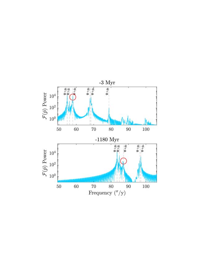
Figure 8: Fast Fourier transform (FFT $={\cal F}(\bar{p})$) of climatic precession $\bar{p}=e\sin\bar{\omega}$ over 6-Myr intervals. Frequencies in arcsec y^-1 = ” y^-1. Note different lunisolar precession frequency $\Psi$ in the past owing to the Earth-Moon system’s evolution (for details and code, see (Zeebe, 2022), github.com/rezeebe/snvec, www2.hawaii.edu/~zeebe/Astro.html, and Section 2.3). Top: Standard spectrum in the recent past centered at $t=-3$ Myr (nearly identical in all solutions). Bottom: Spectrum based on solution R06 centered at $t=-1180$ Myr. Note the split and reduced power of $\Psi+g_{2}$ in bottom vs. top panel (red circles).

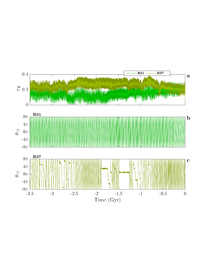
Figure 9: Examples of Mercury’s orbital eccentricity and resonant angle $\theta_{12}$. (a) Mercury’s orbital eccentricity in solutions R01 and R07. The lighter foreground colors represent filter magnitudes ($|z^{*}_{M}|$, see Section 2.5). (b, c) Resonant angle $\mbox{$\theta_{12}$}=(\varpi^{*}_{1}-\varpi^{*}_{2})+(\mbox{$\Omega$}^{*}_{1}-\mbox{$\Omega$}^{*}_{2})$ associated with $\mbox{$\sigma_{12}$}=(g_{1}-g_{2})+(s_{1}-s_{2})$ (see Section 2.5 for calculation). $\theta_{12}$ is intentionally shown over a $16\pi$ range for clarity (at $2\pi$ range, lines connect and appear as areas/patches). (b) $\theta_{12}$ in R01 circulates throughout; $\sigma_{12}$-resonance intervals are absent. (c) $\theta_{12}$ in R07 circulates but also librates during $\sigma_{12}$-resonance intervals (oscillation around a constant value, see e.g., plateau at about $-1.25$ to $-1.5$ Gyr in (c)). Solutions exhibiting $\theta_{12}$-circulation and libration were usually associated with intervals of slightly elevated eccentricity in Mercury’s orbit.

3.3 $\sigma_{12}$ resonance

In a quasi-periodic (non-chaotic) system, the fundamental frequencies are constant over time. In contrast, the solar system’s frequencies change over time owing to dynamical chaos (Fig. 4), priming the system to enter/exit the $\sigma_{12}$ resonance over long time scales. Several solar system resonances have been studied previously, including $(g_{1}-g_{5})-(s_{1}-s_{2})$ and $2(g_{4}-g_{3})-(s_{4}-s_{3})$ (Laskar, 1990; Sussman & Wisdom, 1992; Batygin et al., 2015; Ma et al., 2017; Zeebe, 2022; Abbot et al., 2023). However, to our knowledge only two studies recognized $\sigma_{12}$, yet did not investigate its consequences for $g_{25}$ and Earth’s orbital eccentricity (Lithwick & Wu, 2011; Mogavero & Laskar, 2022). $\sigma_{12}$ may be characterized by the resonant angle $\theta_{12}$ (see Eq. (5)), where $\varpi^{*}$ and $\mbox{$\Omega$}^{*}$ are associated with the $g$- and $s$-modes (analog to longitude of perihelion and ascending node, but not of individual planets, see Appendix A). Chaos is often associated with resonant angles that alternate between circulation and libration (Fig. 9). Generally, $\theta_{12}$ circulated in our solutions without $\sigma_{12}$-resonance episodes, whereas $\theta_{12}$-circulation and libration occurred in solutions that showed $\sigma_{12}$-resonance episodes and a weak/absent LEC. The latter case was usually associated with intervals of slightly elevated eccentricity in Mercury’s orbit ($0.25\ \raisebox{-2.15277pt}{$\stackrel{{\scriptstyle<}}{{\sim}}\ $}\mbox{$e_{\scriptsize\mercury}$}\raisebox{-2.15277pt}{$\stackrel{{\scriptstyle<}}{{\sim}}\ $}0.35$, see Fig. 9).

Importantly, none of our solutions showed high eccentricities ($\mbox{$e_{\scriptsize\mercury}$}\ \raisebox{-2.15277pt}{$\stackrel{{\scriptstyle>}}{{\sim}}\ $}0.4$), which could indicate progressing chaotic behavior or a potential destabilization of the inner solar system — known, separate dynamical phenomena, most relevant to future chaos, studied previously (Laskar, 1990; Sussman & Wisdom, 1992; Lithwick & Wu, 2011; Batygin et al., 2015; Zeebe, 2015; Brown & Rein, 2020; Abbot et al., 2023). Solutions displaying any significant destabilization in the past can of course be excluded (incompatible with the solar system’s known history). Furthermore, given that all our solutions showed at most slightly elevated $e_{\scriptsize\mercury}$ demonstrates that the system can enter/exit the $\sigma_{12}$ resonance without major changes in, or destabilization of, planetary orbits. Thus, past $\sigma_{12}$-resonance episodes and a weak LEC are a possible and likely dynamical phenomenon, present in $\sim$40% of our solutions.

4 Implications

We anticipate far-reaching consequences of our findings for ($i$) exploring the effects of secular resonances (particularly $\sigma_{12}$) on the long-term dynamical evolution, chaos, and planetary climates in the solar system, ($ii$) understanding and unraveling Earth’s past climate forcing and climate change via parameters including eccentricity (total insolation) and climatic precession (see Eq. (7) and Figs. 1, 6, 7, 8), ($iii$) reconstructing the solar system’s chaotic dynamics constrained by geologic evidence (Ma et al., 2017; Meyers & Malinverno, 2018; Zeebe & Lourens, 2019; Olsen et al., 2019), ($iv$) expanding the evidence for the astronomical theory of climate in yet understudied parts of Earth’s history (e.g., the Precambrian), ($v$) studying effects of deep-time Milanković forcing on Earth’s environmental and climatic long-term evolution, and ($vi$) extending the astronomically calibrated geological time scale (Montenari, 2018; Zeebe & Lourens, 2022) into deep time.

It appears that the $\sigma_{12}$ secular resonance and its effect on solar system dynamics and planetary climates has been understudied thus far. To our knowledge, only two studies recognized $\sigma_{12}$, yet did not investigate its consequences on, for instance, ($g_{2}$$-$$g_{5}$) and Earth’s orbital eccentricity (Lithwick & Wu, 2011; Mogavero & Laskar, 2022). Several of the secular modes (or terms) related to the $g_{i}$ and $s_{i}$ (or differences between pairs) show multiple, strong interactions for $i=1,\ldots 4$. In other words, secular resonances usually affect multiple frequency pairs. For example, as shown here, the $\sigma_{12}$ resonance has a major impact on ($g_{1}$$-$$g_{2}$) and ($s_{1}$$-$$s_{2}$), but also on ($g_{2}$$-$$g_{5}$). Moreover, because there is no simple one-to-one relationship between a single mode and a single inner planet (the motion is a superposition of all modes), resonances (say $\sigma_{ij}$ with $i,j=1,\ldots 4$, $i\neq j$) affect the entire inner solar system. Here, we have only investigated $\sigma_{12}$’s effect on ($g_{2}$$-$$g_{5}$) and Earth’s orbital eccentricity. Future work should explore whether there are other important, yet unknown, effects of $\sigma_{12}$ (and other resonances) on the dynamics and planetary climates in the inner solar system.

Our results have fundamental implications for, e.g., current astrochronologic and cyclostratigraphic practices, which are based on the paradigm that the LEC is stable, dominates the eccentricity spectrum, and has a period of $\sim$405 kyr. Given our findings that the $\sigma_{12}$ resonance is a common phenomenon (occurring in $\sim$40% of our solutions), the assumption of a stable 405 kyr cycle in deep time can no longer be made. Specifically, the possibility of an unstable period and weakened LEC amplitude requires rethinking of currently employed strategies for building accurate and high-resolution (‘floating’ or radio-isotopically anchored) astrochronologic age models. The presumed 405-kyr “metronome” was particularly important for constructing pre-Cenozoic age models, where reliable astronomical solutions are absent owing to solar system chaos. Deep-time astrochronologies have thus far critically relied on identification of the LEC because it is the only Milanković cycle whose period has been widely regarded as stable (Laskar et al., 2004; Kent et al., 2018; Spalding et al., 2018) and of sufficiently large amplitude to be typically expressed in sedimentary sequences. Our results indicate that, prior to several hundred Myrs in the past, the LEC may have become unstable over multi-million year intervals. Notably, on these time scales the periods of other critical Milanković parameters (climatic precession and obliquity) are also more uncertain due to changes in the Earth-Moon system’s tidal evolution.

Does the presently explored geologic record provide examples consistent with our astronomical calculations? We note here a recently discovered section in the $\sim$2.46 Ga Joffre Member of the Brockman Iron Formation (Joffre Falls, Western Australia), in which a dominant short eccentricity cycle was reported ($\sim$100 kyr), compared to a relatively weak expression at the scale of the interpreted LEC (Lantink et al., 2022) (see Fig. D.1). The interpreted eccentricity modulation pattern in the Joffre Falls section differs from typical Cenozoic precession-eccentricity dominated records, which often display a strong 1:4 hierarchy of long vs. short eccentricity cycles. One first-order interpretation for the unusual bundling pattern is a complex nonlinear response of the paleoclimate and/or sedimentary system to orbital forcing, which is still poorly understood for the ancient deposits. Yet, given our findings, a fundamentally different pattern of Earth’s orbital eccentricity variations (i.e., a weakened LEC) at the time of deposition provides an alternative explanation (see Fig. D.1). Further investigations are required to confirm past $\sigma_{12}$-resonance episodes in geologic sequences. We propose that future exploration of high-quality and rhythmic sediment successions (especially of Precambrian age) will be critical in constraining the LEC’s past stability and hence the history of the solar system’s chaotic evolution.

Generally, the possibility of an unstable/weak LEC argues strongly for internal consistency checks and tests of eccentricity-related cycles interpreted in stratigraphic sequences at multiple levels. For example, future studies need to include consistency checks between the period of short eccentricity and associated $g$-frequencies and the period of the interpreted $(g_{4}-g_{3})$ cycle and/or other very long period eccentricity modulations. At a more advanced level, the internal consistency of all $g$- and $s$-frequencies that can be extracted from the sequence need to be examined, for which algorithms are already available (Meyers & Malinverno, 2018; Olsen et al., 2019). Furthermore, the uncertainty in LEC stability substantially increases the ambiguity in interpreting cycle ratios of the eccentricity-precession forcing. Hence, independent sedimentation rate checks (preferably from accurate radiometric ages) will become inevitable to verify deep-time Milanković interpretations based on observed stratigraphic cycle hierarchy. Moreover, when significant obliquity signals are present, eccentricity-related cycle pattern will be more difficult to distinguish from those expected for obliquity.

Appendix A $g$- and $s$-modes

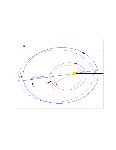
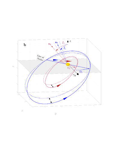
Figure A.1: Schematic illustration of (a) $g$- and (b) $s$-modes (see text).

The $g$- and $s$-modes and their interaction is central for the secular resonances discussed in this study (for illustration, see Fig. A.1). Note that there is generally no simple one-to-one relationship between a single mode and a single planet, though some outer planets may dominate a single mode. $e$, $I$, $\varpi$, and $\Omega$ are eccentricity, inclination, longitude of perihelion, and longitude of ascending node, respectively. $g$-modes are related to $e$ and $\varpi$; $e$ usually varies between some extreme values (black double arrows) and $\varpi$ characterizes the apsidal precession; $\varpi$ may librate (oscillate) or circulate for solar system orbits. The planetary $g_{i}$’s are positive, hence for circulating $\varpi$, the time-averaged apsidal precession is prograde (i.e., in the same direction as the orbital motion, see large colored arrows). The $s$ modes are related to $I$ and $\Omega$; $I$ usually varies between some extreme values (black double arrows) and $\Omega$ characterizes the nodal precession; $\Omega$ may librate or circulate. The planetary $s_{i}$’s are negative, hence for circulating $\Omega$, the time-averaged nodal precession is retrograde (i.e., in the opposite direction as the orbital motion, see large colored arrows). Given conservation of total angular momentum ($L$), there exists an invariable plane perpendicular to $L$, which is fixed in space. It follows that one of the $s$ frequencies is zero ($s_{5}$, see main text).

Appendix B Period of ($g_{2}$$-$$g_{5}$)

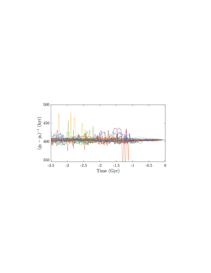
Figure B.1: Period of $\mbox{$g_{25}$}=(g_{2}-g_{5})$ from our ensemble integrations. Solutions including $\sigma_{12}$-resonance intervals ($\sim$40%) are highlighted in color, the remaining solutions are displayed in gray.

The secular frequency $g_{2}$ shows large and rapid shifts (spikes, see Fig. 4) at specific times when the spectral $g_{2}$ peak splits into two peaks at significantly reduced power during $\sigma_{12}$-resonance episodes (see Fig. 5). Alternating maximum power between the two peaks then causes the spikes in $g_{2}$ and hence in $g_{25}$ (Fig. B.1). As a result, $g_{25}$ is unstable and weak/absent during $\sigma_{12}$-resonance intervals. Note that for, e.g., geological applications, the weak/absent LEC is crucial, not the actual value of the $P_{25}$ shift, which is immaterial because it would be unidentifiable in a stratigraphic record owing to the low $g_{25}$ power.

Appendix C Mars’ inclination

The $\sigma_{12}$-resonance motifs are fundamentally different from the recent past (Fig. 6), some of which (coincidentally) show more similarities with Mars’ orbital inclination in the recent past (Fig. C.1) than Earth’s eccentricity.

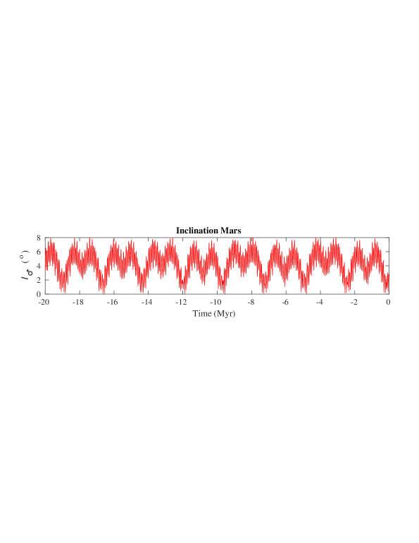
Figure C.1: Mars’ inclination over the past 20 Myr (nearly identical in all solutions, reference frame: ECLIPJ2000).

Appendix D Section at Joffre Falls, Western Australia

In the recently discovered Joffre Falls section ($\sim$2.46 Ga, Western Australia), a dominant short eccentricity cycle was reported ($\sim$100 kyr) and a relatively weak expression of the LEC (Lantink et al., 2022) (see Fig. D.1). The regular medium-scale ($\sim$85 cm) alternations of thicker units of banded iron formation and thinner, softer interval of a more shaley lithology (Fig. D.1, left) have been interpreted as the expression of short eccentricity (Lantink et al., 2022). Horizons highlighted in blue (Fig. D.1, left) correspond to cycle numbers in the original log (Lantink et al., 2022) shown on the right. Note the larger-scale modulations in the thickness and relief of the shaley beds (degree of weathering) forming two distinctive darker ’bundles’ defined by cycles 17-19 and 23-28. This pattern deviates from an expected strong $\sim$1:4 bundling pattern or ratio between the medium- and large-scale cycles in case of a strong and stable LEC. (However, note the $\sim$1:4 ratio visible in the filter amplitude of the bandpass filtered cyclicity on the right.) Higher up in the stratigraphy, the shaley layers become weaker overall and thus any larger-scale modulations are more difficult to recognize. Nevertheless, we count at least 6 medium-scale cycles until the next more distinctive shaley interval, i.e., again no clear 1:4 ratio as would be expected in case of a strong and stable LEC.

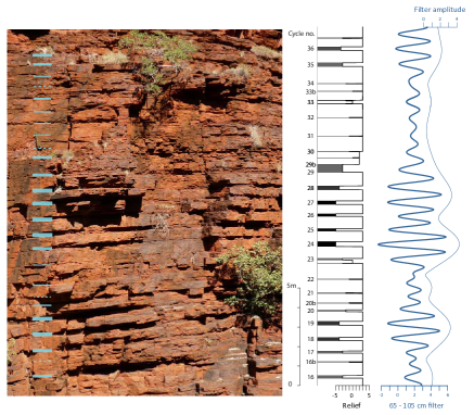
Figure D.1: Section of the $\sim$2.46 Ga Joffre Member exposed at Joffre Falls (Joffre Gorge, Karijini National Park, Western Australia). Photo credit: Frits Hilgen.

References

- Abbot et al. (2023) Abbot, D. S., Hernandez, D. M., Hadden, S., et al. 2023, Astrophys. J., 944, 190, doi: 10.3847/1538-4357/acb6ff
- Batygin & Laughlin (2008) Batygin, K., & Laughlin, G. 2008, Astrophys. J., 683, 1207, doi: 10.1086/589232
- Batygin et al. (2015) Batygin, K., Morbidelli, A., & Holman, M. J. 2015, Astrophys. J., 799, 120, doi: 10.1088/0004-637X/799/2/120
- Berger (1984) Berger, A. 1984, in Milankovitch and Climate: Understanding the Response to Astronomical Forcing, 3–40
- Brown & Rein (2020) Brown, G., & Rein, H. 2020, Res. Notes American Astron. Soc., 4, 221, doi: 10.3847/2515-5172/abd103
- De Vleeschouwer et al. (2024) De Vleeschouwer, D., Percival, L. M., Wichern, N. M., & Batenburg, S. J. 2024, Nature Rev. Earth Env., 5, 59
- De Vleeschouwer, D. (2023) De Vleeschouwer, D. . 2023, Paleoceanogr. Paleoclim., 38, 4555, doi: 10.1029/2022PA004555
- Goldreich (1966) Goldreich, P. 1966, Rev. Geophys. Space Phys., 4, 411, doi: 10.1029/RG004i004p00411
- Hernandez et al. (2022) Hernandez, D. M., Zeebe, R. E., & Hadden, S. 2022, MNRAS, 510, 4302, doi: 10.1093/mnras/stab3664
- Ito & Tanikawa (2002) Ito, T., & Tanikawa, K. 2002, MNRAS, 336, 483, doi: 10.1046/j.1365-8711.2002.05765.x
- Kent et al. (2018) Kent, D. V., Olsen, P. E., Rasmussen, C., et al. 2018, Proc. Nat. Acad. Sci., 115, 6153, doi: 10.1073/pnas.1800891115
- Lantink et al. (2019) Lantink, M. L., Davies, J. H. F. L., Mason, P. R. D., Schaltegger, U., & Hilgen, F. J. 2019, Nature Geosci., 12, 369, doi: 10.1038/s41561-019-0332-8
- Lantink et al. (2022) Lantink, M. L., Davies, J. H. F. L., Ovtcharova, M., & Hilgen, F. J. 2022, Proc. Nat. Acad. Sci., 119, e2117146119, doi: 10.1073/pnas.2117146119
- Laskar (1989) Laskar, J. 1989, Nature, 338, 237, doi: 10.1038/338237a0
- Laskar (1990) —. 1990, Icarus, 88, 266, doi: 10.1016/0019-1035(90)90084-M
- Laskar et al. (2004) Laskar, J., Robutel, P., Joutel, F., et al. 2004, Astron. Astrophys., 428, 261
- Lithwick & Wu (2011) Lithwick, Y., & Wu, Y. 2011, Astrophys. J., 739, 17 pp., doi: 10.1088/0004-637X/739/1/31
- Ma et al. (2017) Ma, C., Meyers, S. R., & Sageman, B. B. 2017, Nature, 542, 468, doi: 10.1038/nature21402
- MacDonald (1964) MacDonald, G. J. F. 1964, Rev. Geophys. Space Phys., 2, 467, doi: 10.1029/RG002i003p00467
- Meyers & Malinverno (2018) Meyers, S. R., & Malinverno, A. 2018, Proceedings of the National Academy of Science, 115, 6363, doi: 10.1073/pnas.1717689115
- Milanković (1941) Milanković, M. 1941, Kanon der Erdbestrahlung und seine Anwendung auf das Eiszeitproblem (Belgrad: Königl. Serb. Akad., pp. 633)
- Mogavero & Laskar (2022) Mogavero, F., & Laskar, J. 2022, Astron. Astrophys., 662, L3, doi: 10.1051/0004-6361/202243327
- Montenari (2018) Montenari, M. 2018, (Editor) Stratigraphy & Timescales: Cyclostratigraphy and Astrochronology in 2018, Vol. 3 (Elsevier), pp. 384
- Morbidelli (2002) Morbidelli, A. 2002, Modern Celestial Mechanics: Aspects of Solar System Dynamics (Taylor & Francis, London)
- Olsen et al. (2019) Olsen, P. E., Laskar, J., Kent, D. V., et al. 2019, Proc. Nat. Acad. Sci., 116, 10664, doi: 10.1073/pnas.1813901116
- OrbitN (2023) OrbitN. 2023, Original Release (Version 1.0.0) 2023, Jun 06 [Software]. Zenodo
- Park et al. (2021) Park, R. S., Folkner, W. M., Williams, J. G., & Boggs, D. H. 2021, Astron. J., 161, 105, doi: 10.3847/1538-3881/abd414
- Poincaré (1914) Poincaré, H. 1914, Science and Method; translated by F. Maitland (Nelson & Sons, London)
- Quinn et al. (1991) Quinn, T. R., Tremaine, S., & Duncan, M. 1991, Astron. J., 101, 2287, doi: 10.1086/115850
- Rauch & Hamilton (2002) Rauch, K. P., & Hamilton, D. P. 2002, in Bull. Am. Astron. Soc., Vol. 34, AAS/Division of Dynamical Astronomy Meeting #33, 938
- Sørensen et al. (2020) Sørensen, A. L., Nielsen, A. T., Thibault, N., et al. 2020, Earth Planet. Sci. Lett., 548, 116475, doi: 10.1016/j.epsl.2020.116475
- Spalding et al. (2018) Spalding, C., Fischer, W. W., & Laughlin, G. 2018, Astrophys. J. Lett., 869, L19, doi: 10.3847/2041-8213/aaf219
- Sussman & Wisdom (1988) Sussman, G. J., & Wisdom, J. 1988, Science, 241, 433, doi: 10.1126/science.241.4864.433
- Sussman & Wisdom (1992) —. 1992, Science, 257, 56, doi: 10.1126/science.257.5066.56
- Touma & Wisdom (1994) Touma, J., & Wisdom, J. 1994, Astron. J., 108, 1943, doi: 10.1086/117209
- Varadi et al. (2003) Varadi, F., Runnegar, B., & Ghil, M. 2003, Astrophys. J., 592, 620, doi: 10.1086/375560
- Wisdom (2015) Wisdom, J. 2015, Astron. J., 150, 127, doi: 10.1088/0004-6256/150/4/127
- Wisdom & Holman (1991) Wisdom, J., & Holman, M. 1991, Astron. J., 102, 1528, doi: 10.1086/115978
- Zeebe (2015) Zeebe, R. E. 2015, Astrophys. J., 811, 9, doi: 10.1088/0004-637X/811/1/9
- Zeebe (2015a) Zeebe, R. E. 2015a, Astrophys. J., 798, 8, doi: 10.1088/0004-637X/798/1/8
- Zeebe (2017) —. 2017, Astron. J., 154, 193, doi: 10.3847/1538-3881/aa8cce
- Zeebe (2022) —. 2022, Astron. J., 164, 107, doi: 10.3847/1538-3881/ac80f8
- Zeebe (2023) Zeebe, R. E. 2023, Astron. J, 166, doi: 10.3847/1538-3881/acd63b
- Zeebe & Lourens (2019) Zeebe, R. E., & Lourens, L. J. 2019, Science, 365, 926
- Zeebe & Lourens (2022) —. 2022, Earth Planet. Sci. Lett., 592, 117595, doi: 10.1016/j.epsl.2022.117595