Radar Rainbow Beams For Wideband mmWave Communication: Beam Training And Tracking

Abstract

We propose a novel integrated sensing and communication (ISAC) system that leverages sensing to assist communication, ensuring fast initial access, seamless user tracking, and uninterrupted communication for millimeter wave (mmWave) wideband systems. True-time-delayers (TTDs) are utilized to generate frequency-dependent radar rainbow beams by controlling the beam squint effect. These beams cover users across the entire angular space simultaneously for fast beam training using just one orthogonal frequency-division multiplexing (OFDM) symbol. Three detection and estimation schemes are proposed based on radar rainbow beams for estimation of the users’ angles, distances, and velocities, which are then exploited for communication beamformer design. The first proposed scheme utilizes a single-antenna radar receiver and one set of rainbow beams, but may cause a Doppler ambiguity. To tackle this limitation, two additional schemes are introduced, utilizing two sets of rainbow beams and a multi-antenna receiver, respectively. Furthermore, the proposed detection and estimation schemes are extended to realize user tracking by choosing different subsets of OFDM subcarriers. This approach eliminates the need to switch phase shifters and TTDs, which are typically necessary in existing tracking technologies, thereby reducing the demands on the control circurity. Simulation results reveal the effectiveness of the proposed rainbow beam-based training and tracking methods for mobile users. Notably, the scheme employing a multi-antenna radar receiver can accurately estimate the channel parameters and can support communication rates comparable to those achieved with perfect channel information.

I Introduction

The integration of sensing and communication (ISAC) has garnered substantial research interest due to the shared characteristics between sensing and communication systems, including signal processing algorithms, system architecture, and spectrum [1, 2, 3]. Sensing targets can be categorized into two groups: cooperative targets with communication needs and non-cooperative targets, including temporarily non-communicating users and obstacles. Sensing can be employed to detect and track both categories of targets. Utilizing bidirectional radar signals for cooperative user detection and location awareness offers advantages, such as enabling pilot- and feedback-free, low-latency communication, over unidirectional training communication signals. Sensing is essential for detecting non-cooperative targets and constructing a channel knowledge map [4]. Such a map is valuable for predicting communication disruptions based on the positions of obstacles and user mobility patterns. It enables proactive selection of alternative communication links, such as non-line-of-sight (NLOS) paths reflected by environmental clutter or reconfigurable intelligent surface (RIS)/relay-aided links, thus supporting resilient communication.

In both communication and radar systems, beam training is of fundamental importance and requires probing beams pointing in different directions sequentially to detect the presence and estimate the positions of users/targets [5]. However, the linear scaling of the required number of beams with the array size gives rise to a large beam training overhead and latency. To enhance training efficiency, two common approaches are employed. The first approach, based on advanced signal processing, is capable of reducing the required number of beams logarithmically with respect to the array size. Methods like hierarchical beam sweeping [6] and side-information-assisted beam training [7] fall into this category. The second approach is based on multi-beam solutions, relying on advanced hardware design [8, 9, 10, 11, 12, 13], to enable simultaneous channel probing. One method in this category is the simultaneous utilization of multiple radio frequency (RF) chains to generate beams pointing in different directions, where different beams scan different non-overlapping sectors [8, 9, 10]. However, this approach incurs high hardware complexity and cost as a large number of RF chains is needed to reduce training time. Alternatively, a cost-effective method is to employ simple true-time-delayers (TTDs), enabling the generation of frequency-dependent beams pointing in different directions by adjusting the TTD delays [12, 11, 13]. This facilitates the creation of multiple frequency-dependent beams covering the entire angular space by utilizing different frequencies. These so-called rainbow beams can be readily generated based on multi-carrier waveforms in millimeter wave (mmWave) systems.

The concept of TTD based rainbow beams, covering the full angular space, was initially introduced in [12] for fast initial access in mmWave systems. Compared with single-carrier beam scanning exploiting the same bandwidth, multi-carrier rainbow beam training may not have a big advantage in terms of training time. However, it does not need to reconfigure phase shifters (PSs) and TTDs [11]. This feature greatly reduces the requirements on the control circuits for beam training in terms of accuracy and switching time, making TTD based rainbow beams an appealing approach, especially in mmWave systems, where sophisticated hardware based solutions are difficult to realize.

There has been some preliminary research on rainbow beam technology. The authors of [13] investigated two TTD architecture candidates, namely analog and hybrid analog-digital arrays, for rainbow beam generation. Building on these initial findings, the authors of [14] extended this technique for user tracking by generating rainbow beams covering a narrow angular range to encompass possible user movements over a short duration. Moreover, by leveraging the functional relationship between the user channel characteristics and user angles and distances in the near field, the authors of [15] and [16] explored near-field rainbow beam technology for fast training and localization, respectively. Recently, rainbow beam technology has also found application in radar systems for the detection of the angles and distances of static targets [17]. Overall, rainbow beam technology has been shown to be effective in determining user/target positions, including angle and distance, in both communication and radar systems. However, the existing work in this area has two primary limitations: 1) The existing literature has primarily focused on static targets and has not considered moving targets and velocity parameter estimation. 2) Prior work has concentrated on the sensing function of rainbow beams, either for detection and tracking of user position parameters using communication signals [12, 13, 14, 15, 16] or detection of target position parameters using radar signals [17]. The application of rainbow beam technology in ISAC systems has not been explored, yet.

Against the above background, this work proposes a novel ISAC architecture aimed at enhancing communication through integration of radar functionality. The considered dual-function radar and communication (DFRC) base station (BS) employs a single RF chain to transmit sensing signals for user detection, estimation, and movement tracking. Leveraging timely and reliable channel information acquired through sensing, the DFRC BS further uses multiple RF chains for communication with multiple users. Considering a mmWave wideband system featuring massive antenna arrays, TTDs are utilized to respectively suppress the beam squint effect for effective communication and harness the beam squint effect for generating massive beams concurrently for sensing. The major contributions of this work can be summerized as follows:

• First, we propose a radar multi-beam transmission scheme based on TTDs and orthogonal frequency-division multiplexing (OFDM) signals. Considering the requirements on angular coverage and the resolution of multiple beams, we derive a mathematical relationship between the required number of subcarriers and the antenna array size to create overlapping rainbow beams. We also establish that the angular resolution of rainbow beams is unaffected by the subcarrier spacing and bandwidth.

• Subsequently, we model the radar rainbow beam echo signal and propose three corresponding detection and estimation schemes. The first scheme employs a single-antenna receiver to capture the echo signal of one set of rainbow beams. It exploits the discrete Fourier transform (DFT) and a one-dimensional search to estimate the central reflection subcarrier frequencies and the corresponding angles of the codebook for the users. The remaining user parameters, including velocity and distance, are successively estimated combining the echoes of the subcarriers adjacent to the central reflection subcarrier. While this scheme minimizes array and signal resource usage, it faces challenges in terms of distance and velocity estimation ambiguities. To address the velocity estimation ambiguity, we introduce a second scheme, which is based on the transmission of two sets of radar rainbow beams and leverages the phase difference between two adjacent OFDM symbols to estimate high velocities, and a third scheme, which employs a multi-antenna receiver to capture the echo of one set of rainbow beams.

• Following this, based on the designed rainbow beams, an efficient tracking scheme is developed by manipulating a selected subset of subcarriers. The resulting codebook-based user tracking does not require the switching of PSs and TTDs, eliminating the need of rapid hardware reconfiguration and the associated time overhead. Moreover, by allocating different frequency bands for tracking and communication, mutual interference between sensing and communication is effectively avoided, facilitating continuous user tracking while maintaining uninterrupted communication.

• Through simulations, we show that, for a single-antenna receiver, the proposed rainbow beam training scheme achieves comparable estimation performance as single-carrier radar systems. Furthermore, our result reveal that the benefits of rainbow beams can be fully leveraged by multi-antenna radar receivers, yielding ultra-high precision for estimation. A 3 dB-beamwidth overlap is shown to be sufficient for rainbow beams to achieve high estimation performance. Moreover, our simulations confirm that all three estimation schemes proposed can effectively track high-velocity, non-linearly moving users, acquiring essential channel information for communication. Notably, the scheme based on a multi-antenna radar receiver offers highly accurate angle information, resulting in nearly ideal communication rates for mobile users.

The remainder of this paper is organized as follows. In Section II, we introduce the system model and discuss the frame structure of the considered ISAC system. In Section III, the design of the proposed rainbow beams is provided. The proposed rainbow beam assisted fast beam training and user tracking schemes are presented in Section IV. Finally, Sections V and VI report our numerical results and conclusions, respectively.

Notations: The following mathematical notations and symbols are used throughout this paper. Vectors and matrices are denoted by boldface lowercase letters and boldface uppercase letters, respectively. $\mathbf{X}^{*}$, $\mathbf{X}^{\mathrm{T}}$, $\mathbf{X}^{\mathrm{H}}$, $\mathbf{X}^{\dagger}$, $||\mathbf{X}||_{F}$, $\mathrm{Tr}\{{\bf X\}}$, and $\mathrm{vec}(\mathbf{X})$ denote the conjugate, transpose, Hermitian (conjugate transpose), pseudo-inverse, Frobenius norm, trace, and vectorization of matrix $\mathbf{X}$, respectively. $||\mathbf{x}||_{2}$ denotes the $l_{2}$-norm of vector $\mathbf{x}$. $\mathfrak{R}\{x\}$ denotes the real part of a complex value. $\mathbb{E}\{\cdot\}$ denotes the expectation of a random variable. $|\cdot|$ and $\angle\left(\cdot\right)$ denote the modulus and angle of a complex number, respectively. $[\mathbf{x}]_{m}$ denotes the $m$-th element of vector $\mathbf{x}$, and $[\mathbf{X}]_{m,n}$ denotes the $(m,n)$-th element of matrix $\mathbf{X}$. The $m$-th row of matrix $\mathbf{X}$ is denoted by $[\mathbf{X}]_{m,:}$. $\odot$ denotes the Hadamard product. $\mathrm{Diag}(\mathbf{x})$ is a diagonal matrix having the entries of vector $\mathbf{x}$ on its main diagonal. Additionally, $\mathbb{C}$ and $\mathbb{R}$ refer to the fields of complex and real numbers, respectively, and $j\triangleq\sqrt{-1}$ is the imaginary unit.

II System Model

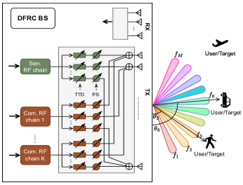
Figure 1: System model of an ISAC system.

In this work, we investigate an ISAC system with a specific focus on sensing-assisted communication, where sensing is exploited for detecting and estimating the users’ directions for the initial access for communication and then tracking the mobile users’ positions for continously updating the estimated angles and gains of the light-of-sight (LoSs) channels, enabling low overhead, high reliability, and low-latency communications.

Specifically, we consider a wideband mmWave massive multiple-input multiple-output (MIMO) system serving $K$ mobile communication users equipped with single antenna. Let $\theta_{k}$, $v_{k}$, and $D_{k}$ denote the angle, velocity, and distance of the $k$-th user relative to the BS, respectively. The DFRC BS is equipped with an $N_{r}$-antenna uniform linear array (ULA) for reception and an $N_{t}$-antenna ULA for transmission, where the two separate antenna arrays are used to suppress the self-interference caused by simultaneous transmission and reception. As shown in Fig. 1, the DFRC BS transmit antenna array is connected to $K$ RF chains providing communication services for $K$ users and an additional RF chain dedicated to sensing. Each RF chain is connected to all $N_{t}$ transmit antennas via $N_{t}$ PSs and $N_{t}$ TTDs.

II-A Signal Model

The considered cyclic prefix (CP)-OFDM system utilizes a total bandwidth of $B_{{\rm tot}}=B_{{\rm sen}}+B_{\mathrm{guard}}+B_{{\rm com}}$, which is partitioned into $B_{{\rm sen}}$ for sensing, $B_{{\rm com}}$ for communication, and $B_{\mathrm{guard}}$ for the frequency guard interval between the sensing and communication frequency bands. This frequency division can effectively avoid mutual interference between concurrently transmitted sensing and communication signals. In addition, bandwidth $B_{{\rm sen}}+B_{\mathrm{guard}}$ can be used to also transmit communication data when sensing is not performed and only communication is activated. We note that different OFDM symbols are modulated separately for sensing and communication.

II-A1 Signal Model for Sensing

The subcarrier spacing of the sensing OFDM signal is $\triangle f_{{\rm sen}}$, resulting in the elementary symbol duration, $T_{{\rm sen}}=1/\triangle f_{{\rm sen}}$. The number of subcarriers is given by $M=B_{{\rm sen}}/\triangle f_{{\rm sen}}+1$ and assumed to be an odd number. The cyclic prefix length satisfies $N_{\mathrm{cp}}=\varrho M$, where $\varrho=1/4\textrm{ or }1/8$ in 5G NR [18]. Define set $\mathcal{M}=\{0,...,M-1\}$. The baseband OFDM sensing signal is given by $\sum_{m\in\mathcal{M}}s_{m}(t)\triangleq\sum_{m\in\mathcal{M}}S_{m}e^{j2\pi f_{m}t}$ [19, Ch. 4.2.1.2], where $f_{m}=-\frac{B_{{\rm sen}}}{2}+m\triangle f_{{\rm sen}}$ is the $m$-th baseband subcarrier frequency and $S_{m}$ is the complex phase-shift keying (PSK) modulated pilot symbol on the $m$-th subcarrier. After being up-coverted with carrier frequency $f_{\mathrm{c}}$, the RF signal for transmission is given by $\sum_{m\in\mathcal{M}}\mathfrak{R}\left\{\tilde{s}_{m}(t)\right\}\triangleq\sum_{m\in\mathcal{M}}\mathfrak{R}\left\{e^{j2\pi f_{\mathrm{c}}t}s_{m}(t)\right\}\triangleq\sum_{m\in\mathcal{M}}\mathfrak{R}\left\{S_{m}e^{j2\pi(f_{\mathrm{c}}+f_{m})t}\right\}$ [19, Ch. 4.2.1.2]. Denoting the transmit (TX) analog precoding vector for the $m$-th subcarrier by $\mathbf{f}_{m}=\mathbf{f}_{\mathrm{PS}}\odot\mathbf{t}_{m}\in\mathbb{C}^{N_{t}\times 1}$ comprising a frequency-independent phase shift vector $\mathbf{f}_{\mathrm{PS}}$ and a frequency-dependent TTD vector $\mathbf{t}_{m}$, the transmitted sensing signal can be expressed as

$$\sqrt{P_{{\rm s}}}\sum_{m\in\mathcal{M}}\mathbf{f}_{m}\mathfrak{R}\left\{S_{m}e^{j2\pi(f_{\mathrm{c}}+f_{m})t}\right\},$$ (1)

where $P_{{\rm s}}$ is the transmit power.

II-A2 Signal Model for Communication

To avoid multi-user interference, we allocate different OFDM subcarriers to different users. In particular, a resource block comprising $Q$ subcarriers and bandwidth $B_{{\rm com}}/K$ is allocated to each user. Specifically, the baseband frequency of the $q$-th subcarrier allocated to the $k$-th user is given by $f_{k,q}^{\rm com}=\frac{B_{{\rm sen}}}{2}+B_{\mathrm{guard}}+(Q(k-1)+q)\triangle f_{\mathrm{com}}$, $1\leq k\leq K$, $1\leq q\leq Q$, where $\triangle f_{\mathrm{com}}$ is the subcarrier spacing for the communication OFDM symbol whose duration of an OFDM symbol including the CP is defined as $T_{\rm sym}^{\rm com}$. It is assumed that the channel between the BS and the $k$-th user follows Rician fading comprising a LoS component and $L_{k}$ NLoS propagation paths. The space-frequency channel response of the $q$-th subcarrier for the $k$-th user on the $j$ OFDM symbol is giving by $\mathbf{h}_{k,q,j}=\sqrt{\frac{\rho_{k}}{\rho_{k}+1}}\alpha_{k,q,j}\mathbf{a}_{N_{t}}\left(\theta_{k},f_{{\rm c}}+f_{k,q}^{\rm com}\right)+\sqrt{\frac{1}{\rho_{k}+1}}\sum_{l=1}^{L_{k}}\alpha_{k,q,l,j}\mathbf{a}_{N_{t}}\left(\theta_{k,l},f_{{\rm c}}+f_{k,q}^{\rm com}\right)$, with $\rho_{k}$ being the Rice factor, $\mathbf{a}_{N_{t}}$ is the steering vector, and $\theta_{k}$ and $\theta_{k,l}$ denoting the angles of departure (AoDs) of the LoS and the $l$-th NLoS path, respectively. Furthermore, $\alpha_{k,q,j}$ and $\alpha_{k,q,l,j}$ represent the frequency-dependent path fading coefficients. For example, for the LoS path, we have $\alpha_{k,q,j}=\alpha_{k}e^{j2\pi{f_{k}^{\mathrm{d,com}}jT_{\rm sym}^{\rm com}}}e^{-j2\pi f_{k,q}^{\rm com}\tau_{k}^{\mathrm{com}}}$ with frequency-independent fading coefficient $\alpha_{k}$, Doppler frequency $f_{k}^{\mathrm{d,com}}=f_{\mathrm{c}}\frac{v_{k}}{c}$, and delay $\tau_{k}^{\mathrm{com}}=\frac{D_{k}}{c}$ for one-way communication. Since the main focus of this paper is the estimation of the angles, velocities, and distances via rainbow beams, for evaluation of the resulting communication performance in Section V, we assume pure analog precoding. The analog precoding vector is given by $\mathbf{w}_{k,q}={\bf w}_{\mathrm{PS},k}\odot\mathbf{t}_{k,q}^{{\rm com}}$ containing a frequency-independent phase shift vector, ${\bf w}_{\mathrm{PS},k}$, and a frequency-dependent TTD vector, $\mathbf{t}_{k,q}^{{\rm com}}$, specific to the $q$-th subcarrier. Then, the achievable data rate of the $k$-th user on the $q$-th subcarrier is given by

$$R_{k,q}=\log_{2}\left(1+\frac{P_{{\rm c},k}}{\sigma_{{\rm c},k}^{2}}|\mathbf{h}_{k,q}^{\mathrm{H}}{\bf w}_{k,q}|^{2}\right),$$ (2)

where $P_{{\rm c},k}$ and $\sigma_{{\rm c},k}^{2}$ are the transmit and noise powers for user $k$ per subcarrier, respectively.

Optimizing $\mathbf{w}_{k,q}$ for rate maximization requires the channel state information (CSI) of $\mathbf{h}_{k,q}$, which is typically obtained via pilot-based channel estimation methods. However, given the rapid time-varying nature of the channels in mobile scenarios and the dominance of the LoS path in high-frequency systems, it is desirable to leverage radar sensing to acquire CSI for the LoS path comprising angle, velocity, and distance. Based on the estimated CSI of the LoS path, $\mathbf{w}_{k,q}$ can be designed by neglecting the NLoS components.

II-B Controllable Beam Squint

Prior to delving into the design of precoding vectors, $\mathbf{f}_{m}$ and $\mathbf{w}_{k,q}$, it is imperative to highlight the frequency-dependent properties of the massive antenna array for wideband mmWave signals, i.e., the beam squint effect. Let us consider the sensing OFDM signal as an example. Consider an angle $\theta\in[0,\pi]$ measured with respect to (w.r.t.) the array plane. The frequency-dependent steering vector in the far field of the array at angle $\theta$ and frequency $f_{m}+f_{\mathrm{c}}$ is given by $\mathbf{a}_{N_{t}}(\theta,f_{\mathrm{c}}+f_{m})=[1,e^{-j2\pi(f_{\mathrm{c}}+f_{m})\frac{d}{c}\cos\theta},\ldots,e^{-j2\pi(N_{t}-1)(f_{\mathrm{c}}+f_{m})\frac{d}{c}\cos\theta}]^{\mathrm{T}}$, where $d$ and $c$ represent the antenna spacing and the speed of light, respectively. When the propagation delay across the array aperture is less than the sampling duration, i.e., $(N_{t}-1)\frac{d}{c}<\frac{1}{B_{{\rm sen}}}$, $\mathbf{a}_{N_{t}}(\theta,f_{m}+f_{\mathrm{c}})$ can be approximated as a narrowband steering vector, i.e., $\mathbf{a}_{N_{t}}(\theta,f_{\mathrm{c}})$ [12]. In contrast, for a given carrier frequency $f_{\mathrm{c}}$, a large number of antennas $N_{t}$ or a large bandwidth $B_{{\rm sen}}$ lead to the beam squint effect. The beam squint effect causes the beams attributed to different subcarriers to be directed towards distinct angles if a frequency-independent precoding vector is employed.

Specifically, define the beampattern of phase shift precoder $\mathbf{f}_{\mathrm{PS}}$ at angle $\theta$ and frequency $f_{m}+f_{\mathrm{c}}$ as $\left|\mathbf{a}_{N_{t}}^{\mathrm{H}}\left(\theta,f_{m}+f_{\mathrm{c}}\right)\mathbf{f}_{\mathrm{PS}}\right|^{2}$. If we let the beam of the center subcarrier, with frequency $f_{\mathrm{c}}$, point towards direction angle $\theta_{\mathrm{c}}$, precoder $\mathbf{f}_{\mathrm{PS}}$ should be chosen as $\mathbf{f}_{\mathrm{PS}}=\mathbf{a}_{N_{t}}\left(\theta_{\mathrm{c}},f_{\mathrm{c}}\right)$, such that $\left|\mathbf{a}_{N_{t}}^{\mathrm{H}}\left(\theta,f_{\mathrm{c}}\right)\mathbf{f}_{\mathrm{PS}}\right|^{2}$ has the maximum value $N_{t}^{2}$ when $\theta=\theta_{\mathrm{c}}$. Given the frequency-independent precoder, the main lobe peak of the beampattern

$$\left|\mathbf{a}_{N_{t}}^{\mathrm{H}}\left(\theta,f_{m}+f_{\mathrm{c}}\right)\mathbf{f}_{\mathrm{PS}}\right|^{2} =\left|\sum_{n=1}^{N_{t}}e^{j2\pi(n-1)\left((f_{\mathrm{c}}+f_{m})\frac{d}{c}\cos\theta-f_{\mathrm{c}}\frac{d}{c}\cos\theta_{\mathrm{c}}\right)}\right|^{2}$$ (3)

for the subcarrier at frequency $f_{m}+f_{\mathrm{c}}$ is located at

$$\theta_{m}^{\mathrm{PS}} =\arccos\left(\frac{f_{\mathrm{c}}}{f_{\mathrm{c}}+f_{m}}\cos\theta_{\mathrm{c}}\right)$$ (4)

satisfying $(f_{\mathrm{c}}+f_{m})\frac{d}{c}\cos\theta_{m}^{\mathrm{PS}}-f_{\mathrm{c}}\frac{d}{c}\cos\theta_{\mathrm{c}}=0$. In narrowband systems with $\frac{f_{m}}{f_{\mathrm{c}}}\ll 1$, a highly focused OFDM beam with one main lobe peak direction at angle $\theta_{\mathrm{c}}$ can be generated to serve the users. However, in wideband systems, the main lobe peak $\theta_{m}^{\mathrm{PS}}$, for non-center carriers, deviates from the desired direction $\theta_{\mathrm{c}}$. This may lead to performance degradation. To control the beam squint effect in wideband communication systems, TTDs are utilized, which introduce constant delays to all subcarriers, resulting in a frequency-dependent steering vector that enables control of the beam direction for different signal frequencies. In this work, we consider the commonly used RF TTDs and denote by $\kappa_{n}=(n-1)\triangle\kappa$ the delay of the delay line for the $n$-th transmit antenna, where $\triangle\kappa$ is the delay spacing between adjacent antennas. This produces frequency-dependent TTD vectors, as $\mathbf{t}_{m}=[1,e^{-j2\pi f_{m}\triangle\kappa},\ldots,e^{-j2\pi f_{m}(N_{t}-1)\triangle\kappa}]^{\mathrm{T}}$. Then, the beampattern of $\mathbf{f}_{m}=\mathbf{f}_{\mathrm{PS}}\odot\mathbf{t}_{m}$ is given by

$$G(\theta,f_{m}) =\left|\mathbf{a}_{N_{t}}^{\mathrm{H}}\left(\theta,f_{m}+f_{\mathrm{c}}\right)(\mathbf{f}_{\mathrm{PS}}\odot\mathbf{t}_{m})\right|^{2}$$

$$=\left|\sum_{n=1}^{N_{t}}e^{j2\pi(n-1)\left((f_{\mathrm{c}}+f_{m})\frac{d}{c}\cos\theta-f_{\mathrm{c}}\frac{d}{c}\cos\theta_{\mathrm{c}}-f_{m}\triangle\kappa\right)}\right|^{2}$$ (5)

with the main lobe peak of subcarrier $m$ pointing to

$$\theta_{m}^{\mathrm{TTD}} =\arccos\left(\frac{\frac{c}{d}f_{m}\triangle\kappa+f_{\mathrm{c}}\cos\theta_{\mathrm{c}}}{f_{\mathrm{c}}+f_{m}}\right).$$ (6)

II-B1 Mitigation of Beam Squint for Communication

For communication, the beam squint effect must be mitigated such that the beams of all subcarriers focus towards the user of interest. This can be achieved by designing the delay parameter as $\triangle\kappa=\frac{d}{c}\cos\theta_{\mathrm{c}}$ such that $\theta_{m}^{\mathrm{TTD}}$ in (6) is independent of $f_{m}$.

II-B2 Utilization of Beam Squint for Sensing

For sensing, the beam squint effect can be strategically harnessed, allowing the beams corresponding to different subcarriers to be concurrently directed toward different directions by properly choosing the TTD vector. The resulting set of OFDM subcarrier beams are called “rainbow beams”, encompassing all potential positions of the sensing targets simultaneously, as elaborated in Section III.

II-C Frame Structure

To establish reliable communication links, accurate information regarding the directions of the users at the BS is essential. Conventionally, beam training is employed by the BS to identify the users’ directions for initial access, achieved through scanning the entire angular space using narrow beams. Subsequently, to maintain the connection, the users’ directions have to be tracked by scanning a smaller angular space that covers the previously identified directions [22]. However, this approach inevitably introduces significant latency and communication overhead, as it necessitates substantial pilot and feedback overhead. The corresponding frame structure is shown in Fig. 3(a). Furthermore, this approach requires frequent and fast switching of the array PSs, which is difficult to realize at high frequencies [13]. To reduce the overhead and hardware complexity, and achieve high-reliability and low-latency communications, we propose a novel scheme comprising fast beam training and continuous user tracking strategies by leveraging the synergies between DFRC and rainbow beamforming. The proposed frame structure for rainbow beam aided ISAC systems is depicted in Fig. 3(b).

1) Beam Training Block: The DFRC BS employs a frequency-dependent TTD array forming rainbow beams based on an OFDM signal. These beams are designed to cover the entire angular space, enabling the detection and estimation of angles, distances, and velocities of communication users.

2) Simultaneous Beam Tracking And Communication Block: The DFRC BS effectively combines the functionalities of downlink communication and movement trajectory sensing. This integrated operation enables the system to perform seamless tracking of users while continuously communicating with them simultaneously in a different frequency band[23]. For communication, the BS designs the communication beamforming based on the previously estimated user angles. Notably, the rainbow beam enabled training conducted during the initial access block is highly efficient, requiring minimal OFDM resources and no hardware overhead for PS and TTD switching. We assume that a user’s direction information obtained in the initial access block remains unchanged during the subsequent radio frames. Furthermore, we approximate the user’s estimated position information derived from radar signal reflection to be equal to its antenna position, valid in far-field communication scenarios where a user with small cross-section area is situated at a considerable distance from the BS and can be treated as a point target [24]. Regarding user tracking, the DFRC-BS employs one RF chain to create multiple rainbow beam sectors, each comprising adjacent subcarrier beams and covering a small angular space, for simultaneous monitoring of multiple users. Users having similar angular directions are tracked within the same sector. Due to the shared time resources between user tracking and communication, the proposed scheme enables uninterrupted communication, leading to enhanced spectral effeciency and reduced system-level communication latency.

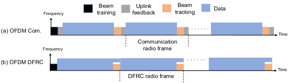
Figure 2: Frame structure of the proposed rainbow beam aided ISAC.

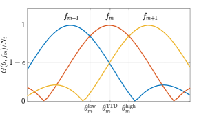
Figure 3: Example of overlapping beams.

III Design of Rainbow Beams for Sensing

In this subsection, the beam squint effect is exploited to realize fast sensing of multiple users. To this end, two essential problems must be tackled for the design of rainbow beams. Firstly, the delays of the TTDs have to be designed to ensure full angular coverage of the beams corresponding to different subcarriers. Secondly, the subcarrier spacing and total number of sensing subcarriers should be determined to guarantee angle resolution, ensuring that any arbitrary angle is covered by at least one subcarrier with sufficient beam gain for robust detection.

III-A Problem 1: Coverage

Let $[\theta_{\mathrm{low}},\theta_{\mathrm{high}}]\subseteq[0,\pi]$ define the angular space covering all potential user directions. The aim of the TTD delay design is to let the beams of all subcarriers $f_{m\in\mathcal{M}}\in[-\frac{B_{{\rm sen}}}{2},\frac{B_{{\rm sen}}}{2}]$ cover the entire angular space. To this end, we let subcarriers $f_{0}=-\frac{B_{{\rm sen}}}{2}$ and $f_{M-1}=\frac{B_{{\rm sen}}}{2}$ points to $\theta_{\mathrm{low}}$ and $\theta_{\mathrm{high}}$, respectively, and obtain the following lemma.

Lemma 1

To sense users within the angular space $[\theta_{\mathrm{low}},\theta_{\mathrm{high}}]\subseteq[0,\pi]$ using a multi-carrier signal with bandwidth $B_{{\rm sen}}$ and carrier frequency $f_{{\rm c}}$, the PSs and TTDs can be designed by determining $\triangle\kappa$ and $\theta_{\mathrm{c}}$ as follows:

$$\triangle\kappa =\frac{1}{2}\left[\left(\frac{1}{B_{{\rm sen}}}+\frac{1}{2f_{\mathrm{c}}}\right)\cos\theta_{\mathrm{high}}-\left(\frac{1}{B_{{\rm sen}}}-\frac{1}{2f_{\mathrm{c}}}\right)\cos\theta_{\mathrm{low}}\right],$$ (7)

$$\theta_{\mathrm{c}} =\arccos\left(\frac{B_{{\rm sen}}}{2}\left[\left(\frac{1}{B_{{\rm sen}}}+\frac{1}{2f_{\mathrm{c}}}\right)\cos\theta_{\mathrm{high}}+\left(\frac{1}{B_{{\rm sen}}}-\frac{1}{2f_{\mathrm{c}}}\right)\cos\theta_{\mathrm{low}}\right]\right).$$ (8)

Proof: Lemma 1 holds under the assumption of half-wavelength antenna spacing, i.e., $\frac{c}{d}=2f_{\mathrm{c}}$, and can be proved by combining $\cos\theta_{\rm low}=\frac{2f_{\mathrm{c}}f_{0}\triangle\kappa+f_{\mathrm{c}}\cos\theta_{\mathrm{c}}}{(f_{\mathrm{c}}+f_{0})}$ and $\cos\theta_{\rm high}=\frac{2f_{\mathrm{c}}f_{M+1}\triangle\kappa+f_{\mathrm{c}}\cos\theta_{\mathrm{c}}}{(f_{\mathrm{c}}+f_{M+1})}$.  $\blacksquare$

III-B Problem 2: Resolution

The resolution of the rainbow beams depends on the total number of subcarriers used. A larger number of subcarriers provides a higher angular resolution, which however causes challenges for detection and estimation due to the associated high sampling rates and main lobe ambiguities. Herein, our initial focus is on ascertaining the minimal required number of subcarriers. To avoid missing users due to uncovered directions, following[12], overlapping beams are needed, such that for any arbitrary direction, at least one subcarrier has adequate beamforming gain. However, compared to [14], the scope of this work is expanded to the estimation of additional parameters such as the users’ distances and velocities. Therefore, the design goal for the overlapping beams is to ensure that, for any arbitrary angle, at least two beams provide a power gain of no less than $(1-\epsilon)N_{t}^{2}$, where $\epsilon\in[0,1]$ is the reduction in power compared to the maximum power, i.e., $N_{t}^{2}$, and is referred to as beam overlap factor in this paper. In other words, any arbitrary angle should be covered by the $\epsilon$-beamwidth of at least two beams. Mathematically, define the angular space $[\theta_{m}^{\mathrm{low}},\theta_{m}^{\mathrm{high}}]$, wherein the beam of $f_{m}$ provides a larger gain compared with the adjacent beams, as shown in Fig. 3. The design problem is to identify the feasible set $\mathcal{S}$ of design parameters, ensuring that within region $[\theta_{m}^{\mathrm{low}},\theta_{m}^{\mathrm{high}}]$, the beam gain of at least one adjacent subcarrier does not drop below $(1-\epsilon)N_{t}^{2}$:

$$\mathcal{S}=\left\{(\triangle f_{{\rm sen}},M)\left|\left(\min_{1\leq m\leq M}\min_{\theta\in[\theta_{m}^{\mathrm{low}},\theta_{m}^{\mathrm{high}}]}\max(G(\theta,f_{m+1}),G(\theta,f_{m-1}))\right)\geq(1-\epsilon)N_{t}^{2}\right.\right\}.$$ (9)

As shown in Fig. 3, for a given $f_{m}$, the main lobes of adjacent subcarriers $f_{m-1}$ and $f_{m+1}$ intersect at the angle of $\theta_{m}^{\mathrm{TTD}}\in[\theta_{m}^{\mathrm{low}},\theta_{m}^{\mathrm{high}}]$, yielding $G(\theta_{m}^{\mathrm{TTD}},f_{m+1})=G(\theta_{m}^{\mathrm{TTD}},f_{m-1})$. This implies that in the angular space $[\theta_{m}^{\mathrm{low}},\theta_{m}^{\mathrm{high}}]$, the minimum gain for the adjacent subcarriers is obtained for $\theta_{m}^{\mathrm{TTD}}$. Then, Problem (9) becomes

$$\mathcal{S}=\left\{(\triangle f_{{\rm sen}},M)\left|\left(\min_{1\leq m\leq M}G(\theta_{m}^{\mathrm{TTD}},f_{m+1})\right)\geq(1-\epsilon)N_{t}^{2}\right.\right\}.$$ (10)

By utilizing (5) and defining

$$\psi(\theta_{m}^{\mathrm{TTD}},f_{m+1}) =(f_{\mathrm{c}}+f_{m+1})\frac{d}{c}\cos\theta_{m}^{\mathrm{TTD}}-f_{\mathrm{c}}\frac{d}{c}\cos\theta_{\mathrm{c}}-f_{m+1}\triangle\kappa$$

$$=\frac{\cos\theta_{\mathrm{c}}-2f_{\mathrm{c}}\triangle\kappa}{2(f_{\mathrm{c}}+f_{m})}\triangle f_{{\rm sen}},$$ (11)

(10) is equivalent to

$$\mathcal{S}=\left\{(\triangle f_{{\rm sen}},M)\left|\left(\max_{1\leq m\leq M}2\pi\left|\psi(\theta_{m}^{\mathrm{TTD}},f_{m+1})\right|\right)\leq\frac{\triangle\psi_{\epsilon}}{2}\right.\right\},$$ (12)

where $\triangle\psi_{\epsilon}$ is the $\epsilon$-beamwidth and can be found numerically [25, Ch. 22.7]. For example, the 3dB-beamwidth is $\triangle\psi_{\mathrm{3dB}}=0.886(2\pi/N_{t})$. The solution of Problem (12) is provided in the following lemma.

Lemma 2

For rainbow beams with beam overlap factor ${\epsilon}$ to cover an angular space of $[\theta_{\mathrm{low}},\theta_{\mathrm{high}}]\subseteq[0,\pi]$ using a multi-carrier signal with bandwidth $B_{{\rm sen}}$ and carrier frequency $f_{{\rm c}}$, the subcarrier spacing and the number of subcarriers need to satisfy

$$\triangle f_{{\rm sen}} \leq\frac{\triangle\psi_{\epsilon}}{4\pi\left(\cos\theta_{\mathrm{c}}\left/(2f_{\mathrm{c}})\right.-\triangle\kappa\right)}=\frac{\triangle\psi_{\epsilon}}{\frac{2\pi}{B_{{\rm sen}}}(1-\frac{B_{{\rm sen}}^{2}}{4f_{\mathrm{c}}^{2}})(\cos\theta_{\mathrm{low}}-\cos\theta_{\mathrm{high}})},$$ (13)

$$M =\frac{B_{{\rm sen}}}{\triangle f_{{\rm sen}}}+1\geq\frac{2\pi(1-\frac{B_{{\rm sen}}^{2}}{4f_{\mathrm{c}}^{2}})(\cos\theta_{\mathrm{low}}-\cos\theta_{\mathrm{high}})}{\triangle\psi_{\epsilon}}+1.$$ (14)

Proof: It is obvious that the maximum value of $\left|\psi(\theta_{m}^{\mathrm{TTD}},f_{m+1})\right|$ is obtained when $f_{m}=0$, leading to

$$\frac{\triangle\psi_{\epsilon}}{2} \geq 2\pi\left|\left(\frac{\cos\theta_{\mathrm{c}}}{2f_{\mathrm{c}}}-\triangle\kappa\right)\triangle f_{{\rm sen}}\right|.$$ (15)

Combining (7) and (8), we have $\frac{\cos\theta_{\mathrm{c}}}{2f_{\mathrm{c}}}-\triangle\kappa=\frac{B_{{\rm sen}}}{2}(\frac{1}{B_{{\rm sen}}^{2}}-\frac{1}{4f_{\mathrm{c}}^{2}})(\cos\theta_{\mathrm{low}}-\cos\theta_{\mathrm{high}})>0$. Therefore, the maximum subcarrier spacing given in (13) can be derived directly from (15).                       $\blacksquare$

For example, for a system with $\frac{B_{{\rm sen}}^{2}}{4f_{\mathrm{c}}^{2}}\ll 1$ and an angular space of $[\theta_{\mathrm{low}},\theta_{\mathrm{high}}]=[0,\pi]$, the critical values for the subcarrier spacing and the required number of subcarriers are $\triangle f_{{\rm sen}}=\frac{\triangle\psi_{\epsilon}B_{{\rm sen}}}{4\pi}$ and $M=\left\lceil 4\pi/\triangle\psi_{\epsilon}\right\rceil+1$, respectively, where ceiling operator $\left\lceil x\right\rceil$ gives the smallest integer that is greater than $x$.

IV Rainbow Beam Training And Tracking

In this section, we first develop a model for the received signal for rainbow beam training, before proposing three parameter estimation schemes. Finally, based on the constructed framework, rainbow beam-based user tracking is established avoiding switching of PSs and TTDs, which are typically necessary in existing tracking technologies.

IV-A Beam Training - Received Signal Model

In this section, we model the echo signal of the rainbow beams emitted by the DFRC BS. Let $m_{k}$ denote the index of the subcarrier reflected by the $k$-th user. To avoid missing any user within the angular space as elaborated in Section III, the sensing rainbow beams must overlap, which causes a given user to be located in the main lobes of the beams created by multiple adjacent subcarriers. We consider a small $N_{r}$ from a cost-effective standpoint, resulting in a frequency-independent receive steering vector $\mathbf{a}_{N_{r}}(\theta_{k})=[1,e^{-j2\pi f_{\mathrm{c}}\frac{d}{c}\cos\theta_{k}},\ldots,e^{-j2\pi(N_{r}-1)f_{\mathrm{c}}\frac{d}{c}\cos\theta_{k}}]^{\mathrm{T}}$. The angle of arrival (AoA), $\theta_{k}$ is identical to the AoD in the transmit steering vector, $\mathbf{a}_{N_{t}}(\theta_{k},f_{m}+f_{\mathrm{c}})$. Define set $\mathcal{M}_{k}$ comprising the indices of the subcarriers whose beams are reflected by the $k$-th user with a relatively high gain, providing useful information for estimation. Collecting the passband echo signal from the $K$ users, the corresponding down-converted complex baseband signal is given by

$${\bf y}(t)=\sum_{k=1}^{K}\mathbf{a}_{N_{r}}\left(\theta_{k}\right)\left(\sum_{m_{k}\in\mathcal{M}_{k}}z_{m_{k}}(t)+\sum_{m_{k}\in\mathcal{M}\setminus\mathcal{M}_{k}}z_{m_{k}}(t)\right)+\mathbf{n}_{r}(t),$$ (16)

where

$$z_{m_{k}}(t) =e^{-j2\pi f_{\mathrm{c}}t}\sqrt{P_{{\rm s}}}\beta_{k}\mathbf{a}_{N_{t}}^{\mathrm{H}}\left(\theta_{k},f_{\mathrm{c}}+f_{m_{k}}\right)\mathbf{f}_{m_{k}}\widetilde{s}_{m_{k}}\left(t-\frac{2(D_{k}-v_{k}t)}{c}\right)$$

$$=\sqrt{P_{{\rm s}}}\beta_{k}\mathbf{a}_{N_{t}}^{\mathrm{H}}\left(\theta_{k},f_{\mathrm{c}}+f_{m_{k}}\right)\mathbf{f}_{m_{k}}e^{j2\pi f_{k}^{\mathrm{d}}t}e^{-j2\pi f_{\mathrm{c}}\tau_{k}}S_{m}e^{j2\pi f_{m_{k}}t}s_{m_{k}}\left(\left(1+\frac{2v_{k}}{c}\right)t-\tau_{k}\right).$$ (17)

Here, $\sum_{m_{k}\in\mathcal{M}_{k}}z_{m_{k}}(t)$ represents the useful echo signal from the subcarriers in $\mathcal{M}_{k}$ and
$\sum_{m_{k}\in\mathcal{M}\setminus\mathcal{M}_{k}}z_{m_{k}}(t)$ is the interference caused by the $k$-th user on the remaining subcarriers. Complex channel gain $\beta_{k}$ comprises the path loss and radar cross section and has power $|\beta_{k}|^{2}=\frac{\lambda_{\mathrm{c}}^{2}\sigma_{\mathrm{rcs}}}{(4\pi)^{3}D_{k}^{4}}$ with radar cross section $\sigma_{\mathrm{rcs}}$ and center carrier wavelength $\lambda_{\mathrm{c}}$. Then, $f_{k}^{\mathrm{d}}=f_{\mathrm{c}}\frac{2v_{k}}{c}$ and $\tau_{k}=\frac{2D_{k}}{c}$ represent the Doppler frequency and round-trip delay of the $k$-th user, respectively. Vector $\mathbf{n}_{r}(t)$ is the additive white Gaussian noise (AWGN) following the distribution $\mathbf{n}_{r}(t)\sim\mathcal{CN}(0,\sigma^{2}_{\rm s}\mathbf{I})$ with noise power $\sigma^{2}_{\rm s}$ at the BS.

The term $(1+\frac{2v_{k}}{c})t$ implies a time stretching/compression of the reflection received from the $k$-th user due to the Doppler effect, giving rise to range migration and Doppler scaling. When the users’ maximum movement within a single OFDM symbol remains significantly less than the distance (range) resolution, i.e., $T_{{\rm sen}}v_{k}\ll c/(2B_{{\rm sen}})$, OFDM radar signal processing techniques typically neglect this effect, adopting the narrowband approximation $s_{m_{k}}((1+\frac{2v_{k}}{c})t-\tau_{k})\approx s_{m_{k}}(t-\tau_{k})$ [1]. This condition is equivalent to a small time-bandwidth product $T_{{\rm sen}}B_{{\rm sen}}\ll\frac{c}{|2v_{k}|}$ and $\left|\frac{2v_{k}}{c}\right|\ll\frac{1}{M}$ [26]. In addition, constant $e^{-j2\pi f_{\mathrm{c}}\tau_{k}}$ can be absorbed into $\tilde{\beta}_{k}=\beta_{k}e^{-j2\pi f_{\mathrm{c}}\tau_{k}}$. With these adjustments, (17) becomes

$$z_{m_{k}}(t) =\sqrt{P_{{\rm s}}}\tilde{\beta}_{k}\mathbf{a}_{N_{t}}^{\mathrm{H}}\left(\theta_{k},f_{\mathrm{c}}+f_{m_{k}}\right)\mathbf{f}_{m_{k}}e^{j2\pi f_{k}^{\mathrm{d}}t}s_{m_{k}}\left(t-\tau_{k}\right).$$ (18)

After matched filtering and sampling at the sampling frequency $M\triangle f_{{\rm sen}}$ at times $t=\frac{nT_{{\rm sen}}}{M}=\frac{n}{M\triangle f_{{\rm sen}}}$, where $n=0,...,M-1$, the discrete-time version of the down-converted signal is obtained as

$${\bf y}[n]=\sum_{k=1}^{K}\mathbf{a}_{N_{r}}\left(\theta_{k}\right)\left(\sum_{m_{k}\in\mathcal{M}_{k}}z_{m_{k}}[n]+\sum_{m_{k}\in\mathcal{M}\setminus\mathcal{M}_{k}}z_{m_{k}}[n]\right)+\mathbf{n}_{r}[n],$$ (19)

where $z_{m_{k}}[n]=\sqrt{P_{{\rm s}}}\tilde{\beta}_{k}\mathbf{a}_{N_{t}}^{\mathrm{H}}\left(\theta_{k},f_{m_{k}}\right)\mathbf{f}_{m_{k}}e^{j2\pi f_{k}^{\mathrm{d}}\frac{nT_{{\rm sen}}}{M}}S_{m_{k}}e^{-j2\pi f_{m_{k}}\tau_{k}}e^{j2\pi(m_{k}-\frac{M-1}{2})\frac{n}{M}}$ and $\mathbf{n}_{r}[n]$ is the discrete-time version of $\mathbf{n}_{r}(t)$.

IV-B Beam Training - Detection and Estimation

In this subsection, we first develop radar detection and estimation algorithms based on a single OFDM symbol and a single-antenna receiver, which can estimate the users’ parameters reliably for low Doppler frequencies but leads to Doppler ambiguity for high Doppler frequencies. To overcome this issue, we propose two alternative schemes that exploit two OFDM symbols and a multi-antenna receiver, respectively.

(1) Single-Antenna Receiver

Assuming a single-antenna receiver, (19) simplifies to ${y}[n]=\sum_{k=1}^{K}\sum_{m_{k}\in\mathcal{M}_{k}}z_{m_{k}}[n]+i[n]+n_{r}[n]$, where $i[n]=\sum_{k=1}^{K}\sum_{m_{k}\in\mathcal{M}\setminus\mathcal{M}_{k}}z_{m_{k}}[n]$ and $n_{r}[n]$ is the AWGN. Collecting samples $y[n]$, $n=0,...,M-1$, in measurement vector $\mathbf{y}=[y[0],y[1],\ldots,y[M-1]]^{{\rm T}}$, we obtain

$$\mathbf{y}\!=\!\mathbf{D}_{M}\!\sum_{k=1}^{K}\!\mathbf{D}(v_{k})\!\sum_{m_{k}\in\mathcal{M}_{k}}\!\!\mathbf{d}_{\mathrm{idft},m_{k}}\tilde{S}_{m_{k}}(\tau_{k})\!\!+\!\mathbf{i}\!+\!\mathbf{n},$$ (20)

where

$$\mathbf{D}_{M}\!=\!\mathrm{Diag}(1,e^{-j\pi(M-1)\frac{1}{M}},\ldots,e^{-j\pi(M-1)\frac{(M-1)}{M}}),$$ (21a)

$$\mathbf{D}(v_{k})\!=\!\mathrm{Diag}(1,\!e^{j2\pi f_{k}^{\mathrm{d}}\frac{T_{{\rm sen}}}{M}},\!\ldots,\!e^{j2\pi f_{k}^{\mathrm{d}}\frac{(M-1)T_{{\rm sen}}}{M}}),$$ (21b)

$$\tilde{S}_{m_{k}}(\tau_{k})\!=\!\sqrt{P_{{\rm s}}}\tilde{\beta}_{k}\mathbf{a}_{N_{t}}^{\mathrm{H}}\left(\theta_{k},f_{m_{k}}\right)\mathbf{f}_{m_{k}}S_{m_{k}}e^{-j2\pi f_{m_{k}}\tau_{k}},$$ (21c)

$$\mathbf{d}_{\mathrm{idft},m_{k}}=[1,e^{j2\pi m_{k}\frac{1}{M}},\ldots,e^{j2\pi m_{k}\frac{(M-1)}{M}}]^{{\rm T}},$$ (21d)

$$\mathbf{i}\!=\![i[0],i[1],\cdots,i[M-1]]^{\mathrm{T}},$$ (21e)

$$\mathbf{n}\!=\![n_{r}[0],n_{r}[1],\cdots,n_{r}[M-1]]^{\mathrm{T}}.$$ (21f)

Here, element $e^{j2\pi f_{k}^{\mathrm{d}}\frac{nT_{{\rm sen}}}{M}}$ of diagonal matrix $\mathbf{D}(v_{k})$ represents the intrapulse Doppler effect, and vector $\mathbf{d}_{\mathrm{idft},m_{k}}$ is the $m_{k}$-th column of the inverse DFT (IDFT) matrix of dimension $M$. The user parameters of interest are included in $\mathbf{D}(v_{k})$, $\tilde{S}_{m_{k}}(\tau_{k})$, and $\mathbf{d}_{\mathrm{idft},m_{k}}$.

A given user reflects signals at different frequencies, each with a different reflection gain. The frequency yielding the highest reflection gain can be regarded as the central reflection frequency of the $k$-th user, denoted as $f_{k_{\mathrm{c}}}$, where $k_{\mathrm{c}}\in\mathcal{M}_{k}$. The angle corresponding to the main lobe peak is regarded as the estimated angle of the $k$-th user. In the subsequent radar detection process, the first step is to segregate the signal components at different frequencies within the echo signal in (20). Thus, we determine the user angles based on the frequency index and proceed to estimate the users’ distance and velocity parameters from the isolated subcarrier-specific echo signals. To this end, we define

$$\tilde{\mathbf{d}}_{\mathrm{idft},m_{k}}(v_{k})=\mathbf{D}(v_{k})\mathbf{d}_{\mathrm{idft},m_{k}},$$ (22)

and rewrite (20) as

$$\mathbf{y} =\mathbf{D}_{M}\sum_{k=1}^{K}\sum_{m_{k}\in\mathcal{M}_{k}}\tilde{\mathbf{d}}_{\mathrm{idft},m_{k}}(v_{k})\tilde{S}_{m_{k}}(\tau_{k})+\mathbf{i}+\mathbf{n}.$$ (23)

(1.1) Single-Antenna Receiver for Low Doppler Frequencies

Under the condition of low Doppler frequencies, bounded by half of the subcarrier spacing, i.e., $|f_{k}^{\mathrm{d}}|<\triangle f_{{\rm sen}}/2$, resulting in a user velocity constraint of $|v_{k}|<\frac{c\triangle f_{{\rm sen}}}{4f_{\mathrm{c}}}$, DFT can be used to estimate the central reflection frequency associated with each user [1]. In particular, by taking the DFT of $\mathbf{y}$, one obtains

$$\mathbf{y}_{\mathrm{DFT}} =\mathbf{D}_{\mathrm{dft}}\mathbf{D}_{M}^{-1}\mathbf{y}$$

$$=\mathbf{D}_{\mathrm{dft}}\!\!\left(\!\sum_{k=1}^{K}\!\sum_{m_{k}\in\mathcal{M}_{k}}\!\!\!\!\tilde{\mathbf{d}}_{\mathrm{idft},m_{k}}(v_{k})\tilde{S}_{m_{k}}(\tau_{k})\!+\!\mathbf{D}_{M}^{-1}(\mathbf{i}\!+\!\mathbf{n})\right)\!,$$ (24)

where the dimension of DFT matrix $\mathbf{D}_{\mathrm{dft}}$ is $M$, and the noise-free version of vector $\mathbf{y}_{\mathrm{DFT}}$ contains $\sum_{k=1}^{K}|\mathcal{M}_{k}|$ nonzero values at row indices $\bigcup_{k=1}^{K}\mathcal{M}_{k}$. Since the subcarrier representing the central reflection frequency $f_{k_{\mathrm{c}}}$ has a higher reflection gain compared to the other subcarriers in $\mathcal{M}_{k}$, a one-dimensional search can be effectively applied to identify the $K$ row indices correspongding to power peaks in $\mathbf{y}_{\mathrm{DFT}}$. These $K$ row indices serve as estimates for the indices of the central reflection frequencies, and the corresponding angles in the codebook of the rainbow beams serve as estimates of the user direction angles, denoted by $\hat{\theta}_{k}$. Note that the intrapulse Doppler effect $e^{j2\pi f_{k}^{\mathrm{d}}\frac{nT_{{\rm sen}}}{M}}$ does not cause an estimation error for the central reflection frequencies, as the subcarriers are not shifted to adjacent subcarrier frequencies owing to the assumption of a low Doppler frequency, i.e., $|f_{k}^{\mathrm{d}}|<\triangle f_{{\rm sen}}/2$. However, errors in user angle estimation may arise due to a mismatch between the discrete angles in the codebook of the rainbow beam and the continuous user angles. This error can be reduced by increasing the number of subcarriers.

Based on the estimate of $f_{k_{\mathrm{c}}}$, denoted by $f_{\hat{k}_{\mathrm{c}}}$, the Doppler frequencies and delays can be estimated by formulating the following problem:

$$\min_{\{v_{k},\mathbf{s}_{k}(\tau_{k})\}_{k=1}^{K}}\left\|\mathbf{D}_{M}^{-1}\mathbf{y}-\sum_{k=1}^{K}\mathbf{D}(v_{k})\mathbf{D}_{\mathrm{idft},k}\mathbf{s}_{k}(\tau_{k})\right\|,$$ (25)

where matrix $\mathbf{D}_{\mathrm{idft},k}\in\mathbb{C}^{M\times|\mathcal{M}_{k}|}$ has $\mathbf{d}_{\mathrm{idft},m_{k}},m_{k}\in\mathcal{M}_{k}$, in (21d) as its columns in ascending order of $m_{k}$ and vector $\mathbf{s}_{k}(\tau_{k})\in\mathbb{C}^{|\mathcal{M}_{k}|\times 1}$ contains the corresponding $\tilde{S}_{m_{k}}(\tau_{k}),m_{k}\in\mathcal{M}_{k}$, given in (21c) as elements in decending order of $m_{k}$.

In order to solve problem (25) efficiently, we assume that the interference between the users is weak, i.e., non-overlapping sets $\mathcal{M}_{k_{1}}\cap\mathcal{M}_{k_{2}}\neq\emptyset$ for $k_{1}\neq k_{2}$. Assuming further a large $M$, we obtain the approximation $\mathbf{D}_{\mathrm{idft},k_{1}}^{\mathrm{H}}\mathbf{D}^{\mathrm{H}}(v_{k_{1}})\mathbf{D}(v_{k_{2}})\mathbf{D}_{\mathrm{idft},k_{2}}\approx\mathbf{I}$ for $k_{1}\neq k_{2}$, where $\mathbf{I}$ is the identity matrix. Given $\{v_{k}\}_{k=1}^{K}$, the optimal estimate for $\{\mathbf{s}_{k}(\tau_{k})\}_{k=1}^{K}$ based on (25) is obtained as

$$\hat{\mathbf{s}}_{k}(\tau_{k})=\left(\mathbf{D}_{\mathrm{idft},k}^{\mathrm{H}}\mathbf{D}_{\mathrm{idft},k}\right)^{-1}\mathbf{D}_{\mathrm{idft},k}^{\mathrm{H}}\mathbf{D}^{\mathrm{H}}(v_{k})\mathbf{D}_{M}^{-1}\mathbf{y},\forall k.$$ (26)

Inserting (26) into Problem (25), the $\{v_{k}\}_{k=1}^{K}$ can be obtained as

$$\{\hat{v}_{k}\}_{k=1}^{K}=\mathrm{arg}\min_{\{v_{k}\}_{k=1}^{K}}\sum_{k=1}^{K}||\mathbf{y}^{H}\left(\mathbf{D}_{M}^{\mathrm{H}}\right)^{-1}\mathbf{D}(v_{k})\mathbf{D}_{\mathrm{idft},k}||^{2}.$$ (27)

Conveniently Problem (27) can be decomposed into $K$ independent subproblems, i.e.,
$\min_{v_{k}}||\mathbf{y}^{H}\left(\mathbf{D}_{M}^{\mathrm{H}}\right)^{-1}\mathbf{D}(v_{k})\mathbf{D}_{\mathrm{idft},k}||^{2},\forall k$, which can be solved through a one-dimensional search in interval $v_{k}\in[-\frac{1}{2},\frac{1}{2}]\frac{c}{2f_{\mathrm{c}}T_{{\rm sen}}}$ in parallel.

Next, for estimation of the delay, from (21c) we obain the following relationship

$$e^{j2\pi\triangle f_{{\rm sen}}\tau_{k}} =\frac{\tilde{S}_{m_{k}}(\tau_{k})\left/\left(\mathbf{a}_{N_{t}}^{\mathrm{H}}\left(\theta_{k},f_{\mathrm{c}}+f_{m_{k}}\right)\mathbf{f}_{m_{k}}S_{m_{k}}\right)\right.}{\tilde{S}_{m_{k}+1}(\tau_{k})\left/\left(\mathbf{a}_{N_{t}}^{\mathrm{H}}\left(\theta_{k},f_{\mathrm{c}}+f_{m_{k}+1}\right)\mathbf{f}_{m_{k}+1}S_{m_{k}+1}\right)\right.},$$ (28)

which implies that the delay estimate, denoted as $\hat{\tau}_{k}$, can be readily obtained once the scalar values $\tilde{S}_{m_{k}}(\tau_{k})$ for two subcarriers from set $\mathcal{M}_{k}$ are known. To maximize estimation accuracy, it is natural to select the two subcarriers with the highest reflection gains from $\mathcal{M}_{k}$, namely the central reflection frequency $f_{k_{\mathrm{c}}}$ and an adjacent subcarrier ($f_{k_{\mathrm{c}}+1}$ or $f_{k_{\mathrm{c}}-1}$) denoted as $f_{k_{\mathrm{c}}\pm 1}$. Then, according to (26), we have

$$\hat{\tilde{S}}_{\hat{k}_{\mathrm{c}}}(\tau_{k}) =\frac{1}{M}[\mathbf{D}_{\mathrm{dft}}]_{\hat{k}_{\mathrm{c}},:}\mathbf{D}^{\mathrm{H}}(\hat{v}_{k})\mathbf{D}_{M}^{-1}\mathbf{y},$$ (29a)

$$\hat{\tilde{S}}_{\hat{k}_{\mathrm{c}}\pm 1}(\tau_{k}) =\frac{1}{M}[\mathbf{D}_{\mathrm{dft}}]_{\hat{k}_{\mathrm{c}}\pm 1,:}\mathbf{D}^{\mathrm{H}}(\hat{v}_{k})\mathbf{D}_{M}^{-1}\mathbf{y},$$ (29b)

due to the orthogonality of OFDM subcarriers. Based on (28) and (29), we obtain the estimate

$$\hat{\tau}_{k} =\pm\frac{1}{2\pi\triangle f_{{\rm sen}}}\angle\left(\frac{\hat{\tilde{S}}_{\hat{k}_{\mathrm{c}}}(\tau_{k})\left/\left(N_{t}S_{\hat{k}_{\mathrm{c}}}\right)\right.}{\hat{\tilde{S}}_{\hat{k}_{\mathrm{c}}\pm 1}(\tau_{k})\left/\left(\mathbf{a}_{N_{t}}^{\mathrm{H}}\left(\hat{\theta}_{k},f_{\mathrm{c}}+f_{\hat{k}_{\mathrm{c}}\pm 1}\right)\mathbf{f}_{\hat{k}_{\mathrm{c}}\pm 1}S_{\hat{k}_{\mathrm{c}}\pm 1}\right)\right.}\right),$$ (30)

where we exploited $N_{t}=\mathbf{a}_{N_{t}}^{\mathrm{H}}\left(\hat{\theta}_{k},f_{\mathrm{c}}+f_{\hat{k}_{\mathrm{c}}}\right)\mathbf{f}_{\hat{k}_{\mathrm{c}}}$ since precoding vector $\mathbf{f}_{\hat{k}_{\mathrm{c}}}$ is designed to align with the steering vector in direction $\hat{\theta}_{k}$.

(1.2) Single-Antenna Receiver for High Doppler Frequencies

In scenarios involving high-speed movement, Doppler ambiguity occurs when the absolute value of the Doppler frequency is greater than half of the subcarrier spacing, i.e., $|f_{k}^{\mathrm{d}}|\geq\triangle f_{{\rm sen}}/2$. This Doppler ambiguity affects $\tilde{\mathbf{d}}_{\mathrm{idft},m_{k}}(v_{k})$ in (22). To elaborate, let $f_{k}^{\mathrm{d}}T_{{\rm sen}}$ be divided into $f_{k}^{\mathrm{d}}T_{{\rm sen}}=\varepsilon_{\mathrm{i},k}+\varepsilon_{\mathrm{f},k}$, where $\varepsilon_{\mathrm{i},k}$ is the integer component and $\varepsilon_{\mathrm{f},k}$ is the fractional component such that $-1/2\leq\varepsilon_{\mathrm{f},k}<1/2$. $\varepsilon_{\mathrm{i},k}$ shifts the frequency $f_{m_{k}}$ to $f_{m_{k}+\varepsilon_{\mathrm{i},k}}$ at the receiver. This may introduce Doppler ambiguity if the shift, $\varepsilon_{\mathrm{i},k}$, is not correctly estimated. The DFT-based method proposed in the previous subsection cannot resolve this Doppler ambiguity. To tackle this issue, an alternative method exploiting two OFDM symbols is proposed, where the Doppler frequency can be estimated by utilizing the interpulse Doppler effect.

Define the OFDM block duration as $T_{\mathrm{sym}}=T_{\mathrm{cp}}+T_{{\rm sen}}$, where $T_{\mathrm{cp}}$ is the CP duration, which limits the maximum detection distance, denoted as $R_{\mathrm{max}}$, as $\frac{2R_{\mathrm{max}}}{c}\leq T_{\mathrm{cp}}$. The first OFDM symbol is given by $\sum_{m\in\mathcal{M}}s_{m}(t)$ as before. The second OFDM symbol is expressed as $\sum_{m\in\mathcal{M}}s_{m}^{(2)}(t-T_{\mathrm{sym}})\triangleq\sum_{m\in\mathcal{M}}S_{m}^{(2)}e^{j2\pi f_{m}(t-T_{\mathrm{sym}})}$, where $S_{m}^{(2)}$ is the pilot symbol on the $m$-th subcarrier of the second OFDM symbol. Following the same signal processing steps as for the first OFDM symbol and removing the CP, for a single-antenna receiver, the received down-converted baseband signal corresponding to (16) is given by $y^{(2)}(t)=\sum_{k=1}^{K}\left(\sum_{m_{k}\in\mathcal{M}_{k}}z^{(2)}_{m_{k}}(t)+\sum_{m_{k}\in\mathcal{M}\setminus\mathcal{M}_{k}}z^{(2)}_{m_{k}}(t)\right)+n^{(2)}(t)$, where $z^{(2)}_{m_{k}}(t)=\sqrt{P_{{\rm s}}}\tilde{\beta}_{k}\mathbf{a}_{N_{t}}^{\mathrm{H}}\left(\theta_{k},f_{\mathrm{c}}+f_{m_{k}}\right)\mathbf{f}_{m_{k}}e^{j2\pi f_{k}^{\mathrm{d}}t}s^{(2)}_{m_{k}}\left(t-T_{\mathrm{sym}}-\tau_{k}\right)$ and $n^{(2)}(t)$ is the AWGN.

We sample the matched filtered $y^{(2)}(t)$ at times $t=T_{\mathrm{sym}}+\frac{nT_{{\rm sen}}}{M}$, and obtain the discrete-time signal as

$$y^{(2)}[n]=\sum_{k=1}^{K}\left(\sum_{m_{k}\in\mathcal{M}_{k}}z^{(2)}_{m_{k}}[n]+\sum_{m_{k}\in\mathcal{M}\setminus\mathcal{M}_{k}}z^{(2)}_{m_{k}}[n]\right)+n^{(2)}[n],$$ (31)

where $z^{(2)}_{m_{k}}[n]=\sqrt{P_{{\rm s}}}\tilde{\beta}_{k}\mathbf{a}_{N_{t}}^{\mathrm{H}}\left(\theta_{k},f_{\mathrm{c}}+f_{m_{k}}\right)\mathbf{f}_{m_{k}}e^{j2\pi f_{k}^{\mathrm{d}}\frac{nT_{{\rm sen}}}{M}}e^{j2\pi f_{k}^{\mathrm{d}}T_{\mathrm{sym}}}S_{m_{k}}^{(2)}e^{-j2\pi f_{m_{k}}\tau_{k}}e^{j2\pi m_{k}\frac{n}{M}}$ and
$e^{j2\pi f_{k}^{\mathrm{d}}T_{\mathrm{sym}}}$ represents the interpulse Doppler effect. Furthermore, for the second OFDM symbol, (23) becomes

$$\mathbf{y}^{(2)} =\mathbf{D}_{M}\sum_{k=1}^{K}\sum_{m_{k}\in\mathcal{M}_{k}}\tilde{\mathbf{d}}_{\mathrm{idft},m_{k}}(v_{k})\tilde{S}_{m_{k}}^{(2)}(\tau_{k},v_{k})+\mathbf{i}^{(2)}+\mathbf{n}^{(2)},$$ (32)

where $\tilde{S}_{m_{k}}^{(2)}(\tau_{k},v_{k})=\sqrt{P_{{\rm s}}}\tilde{\beta}_{k}\mathbf{a}_{N_{t}}^{\mathrm{H}}\left(\theta_{k},f_{\mathrm{c}}+f_{m_{k}}\right)\mathbf{f}_{m_{k}}S_{m_{k}}^{(2)}e^{-j2\pi f_{m_{k}}\tau_{k}}e^{j2\pi f_{k}^{\mathrm{d}}T_{\mathrm{sym}}}$, and $\mathbf{i}^{(2)}$ and $\mathbf{n}^{(2)}$ are the interference from the sidelobes and the AWGN, respectively. Now, the Doppler frequency can be obtained by comparing the phase difference between $\tilde{S}_{m_{k}}(\tau_{k})$ in (21c) and $\tilde{S}_{m_{k}}^{(2)}(\tau_{k},v_{k})$, given by

$$e^{j2\pi f_{k}^{\mathrm{d}}T_{\mathrm{sym}}} =\frac{\tilde{S}_{m_{k}}^{(2)}(\tau_{k},v_{k})/S_{m_{k}}^{(2)}}{\tilde{S}_{m_{k}}(\tau_{k})/S_{m_{k}}}.$$ (33)

Therefore, for the first and second OFDM symbols, the DFT and phase rotation techniques are used to estimate $k_{\mathrm{c}}+\varepsilon_{\mathrm{i},k}$ and $\varepsilon_{\mathrm{f},k}$, respectively. Defining $\hat{k}_{\mathrm{c+i}}$ and $\hat{\varepsilon}_{\mathrm{f},k}$ as the estimates of $k_{\mathrm{c}}+\varepsilon_{\mathrm{i},k}$ and $\varepsilon_{\mathrm{f},k}$, respectively, and following (29a), we obtain the estimates

$$\hat{\tilde{S}}_{\hat{k}_{\mathrm{c+i}}}(\tau_{k}) =\frac{1}{M}[\mathbf{D}_{\mathrm{dft}}]_{\hat{k}_{\mathrm{c+i}},:}\mathbf{D}^{\mathrm{H}}\left(\frac{c\hat{\varepsilon}_{\mathrm{f},k}}{2f_{\mathrm{c}}T_{{\rm sen}}}\right)\mathbf{D}_{M}^{-1}\mathbf{y},$$ (34a)

$$\hat{\tilde{S}}_{\hat{k}_{\mathrm{c+i}}}^{(2)}(\tau_{k},v_{k}) =\frac{1}{M}[\mathbf{D}_{\mathrm{dft}}]_{\hat{k}_{\mathrm{c+i}},:}\mathbf{D}^{\mathrm{H}}\left(\frac{c\hat{\varepsilon}_{\mathrm{f},k}}{2f_{\mathrm{c}}T_{{\rm sen}}}\right)\mathbf{D}_{M}^{-1}\mathbf{y}^{(2)}.$$ (34b)

According to (33) and utilizing (34), we have

$$\hat{f}_{k}^{\mathrm{temp}} =\frac{1}{2\pi T_{\mathrm{sym}}}\angle\left(\frac{\hat{\tilde{S}}_{\hat{k}_{\mathrm{c+i}}}^{(2)}(\tau_{k},v_{k})\left/S_{\hat{k}_{\mathrm{c+i}}}^{(2)}\right.}{\hat{\tilde{S}}_{\hat{k}_{\mathrm{c+i}}}(\tau_{k})\left/S_{\hat{k}_{\mathrm{c+i}}}\right.}\right).$$ (35)

Note that $e^{j2\pi f_{k}^{\mathrm{d}}T_{\mathrm{sym}}}$ is a periodic function of $f_{k}^{\mathrm{d}}T_{\mathrm{sym}}$ with period 1, so $\hat{f}_{k}^{\mathrm{temp}}$ may not be the estimate of $f_{k}^{\mathrm{d}}$. The estimate for the Doppler frequency, denoted by $\hat{f}_{k}^{\mathrm{d}}$, is obtained based on the following analysis. 1) For $0\leq f_{k}^{\mathrm{d}}T_{\mathrm{sym}}=\varepsilon_{\mathrm{f},k}<1/2$, resulting in estimates $\hat{f}_{k}^{\mathrm{temp}}T_{\mathrm{sym}}>0$ and $\hat{\varepsilon}_{\mathrm{f},k}>0$ with $\left|\hat{f}_{k}^{\mathrm{d}}T_{\mathrm{sym}}-\hat{\varepsilon}_{\mathrm{f},k}\right|\rightarrow 0$, then we have $\hat{f}_{k}^{\mathrm{d}}=\hat{f}_{k}^{\mathrm{temp}}$. 2) For $1/2\leq f_{k}^{\mathrm{d}}T_{\mathrm{sym}}=1+\varepsilon_{\mathrm{f},k}<1$, we obtain estimates $\hat{f}_{k}^{\mathrm{temp}}T_{\mathrm{sym}}<0$ and $-1/2<\hat{\varepsilon}_{\mathrm{f},k}<0$, but $\hat{\varepsilon}_{\mathrm{f},k}$ is inaccurate due to the failure of angle rotation method at high Doppler frequency, resulting in $\left|\hat{f}_{k}^{\mathrm{d}}T_{\mathrm{sym}}-\hat{\varepsilon}_{\mathrm{f},k}\right|\gg 0$. Hence, we obtain $\hat{f}_{k}^{\mathrm{d}}T_{\mathrm{sym}}=\hat{f}_{k}^{\mathrm{temp}}T_{\mathrm{sym}}+1$. 3) For $1\leq f_{k}^{\mathrm{d}}T_{\mathrm{sym}}=1+\varepsilon_{\mathrm{f},k}<3/2$, we acquire estimate $\hat{f}_{k}^{\mathrm{d}}T_{\mathrm{sym}}>0$ and inaccurate estimate $1/2>\hat{\varepsilon}_{\mathrm{f},k}>0$, leading to $\left|\hat{f}_{k}^{\mathrm{d}}T_{\mathrm{sym}}-\hat{\varepsilon}_{\mathrm{f},k}\right|\gg 0$, then we have $\hat{f}_{k}^{\mathrm{d}}T_{\mathrm{sym}}=\hat{f}_{k}^{\mathrm{temp}}T_{\mathrm{sym}}+1$. Therefore, the esitmate $\hat{f}_{k}^{\mathrm{d}}$ can be summarized as

$$\hat{f}_{k}^{\mathrm{d}}=\begin{cases}\hat{f}_{k}^{\mathrm{temp}},&\textrm{if }\left|\hat{f}_{k}^{\mathrm{d}}T_{\mathrm{sym}}-\hat{\varepsilon}_{\mathrm{f},k}\right|<\epsilon,\\ \frac{\hat{f}_{k}^{\mathrm{temp}}T_{\mathrm{sym}}+1}{T_{\mathrm{sym}}},&\textrm{if }\left|\hat{f}_{k}^{\mathrm{d}}T_{\mathrm{sym}}-\hat{\varepsilon}_{\mathrm{f},k}\right|\geq\epsilon,\end{cases}$$ (36)

where $\epsilon$ is a threshold and can be empirically set to 0.05. For example, assuming a system with $f_{\mathrm{c}}=100$ GHz, $\triangle f_{{\rm sen}}=240$ kHz, and $T_{\mathrm{sym}}=\frac{5}{4}T_{{\rm sen}}$, the maximum velocity that can be estimated based on (36) is 432 m/s, which is sufficient for all civilian mobile devices. The maximum velocity can be further increased by using a lower central frequency or a larger subcarrier spacing.

The index of the central reflection frequency for the $k$-th user can be obtained as

$$\hat{k}_{\mathrm{c}} =\left\lfloor\hat{k}_{\mathrm{c+i}}+\hat{\varepsilon}_{\mathrm{f},k}-\hat{f}_{k}^{\mathrm{d}}\right\rceil,$$ (37)

where the operation $\left\lfloor\cdot\right\rceil$ rounds towards the nearest integer, which ensures that $\hat{k}_{\mathrm{c}}$ is not affected by the inaccurate estimate $|\hat{\varepsilon}_{\mathrm{f},k}|<1/2$. Once the estimate $\hat{k}_{\mathrm{c}}$ has been determined, the corresponding angles can be obtained from the rainbow beam codebook and the resulting delays can be derived from (29b) and (30).

(2) Multi-Antenna Receiver

Given the fleeting nature of real-time location data for high-speed mobile users, the previous approach, exploiting two OFDM symbols for training, is suboptimal. To reduce the training time overhead inherent to user detection, a multi-antenna receiver is considered as it introduces additional degrees of freedom for estimation. In particular, the user angle can be estimated first by exploiting the diversity gain introduced by multiple antennas, thereby determining the central reflection frequency, $\mathbf{f}_{m_{k}}$. Then, $\varepsilon_{\mathrm{i},k}$ can be acquired once $\mathbf{f}_{m_{k}+\varepsilon_{\mathrm{i},k}}$ has been obtained.

By defining $\bm{\theta}=[\theta_{1},...,\theta_{K}]^{\mathrm{T}}$ and $r_{k}[n]=\sum_{m_{k}\in\mathcal{M}_{k}}z_{m_{k}}[n]+\sum_{m_{k}\in\mathcal{M}\setminus\mathcal{M}_{k}}z_{m_{k}}[n]$, we rewrite (19) for the multi-antenna receiver in compact form as follows

$$\mathbf{y}[n]=\mathbf{A}_{N_{r}}(\bm{\theta})\mathbf{r}[n]+\mathbf{n}_{r}[n],$$ (38)

where $\mathbf{A}_{N_{r}}(\bm{\theta})=[\mathbf{a}_{N_{r}}(\theta_{1}),\ldots,\mathbf{a}_{N_{r}}(\theta_{K})]$ and $\mathbf{r}[n]=[r_{1}[n],\ldots,r_{K}[n]]^{\mathrm{T}}$. Determining $\bm{\theta}$ from (38) is a typical angle estimation problem [27], which can be solved through either grid-on estimation methods (including DFT and orthogonal matching pursuit (OMP) [28]), characterized by low complexity, or gridless estimation methods (including multiple signal classification (MUSIC) [29] and atomic norm minimization (ANM) [30]), known for their high precision. The grid-on estimation methods yield sufficient estimation accuracy for large $N_{r}$. However, considering the limitation of a small $N_{r}$, which can reduce hardware cost and avert the beam squint effect at the receiving array, we adopt the high-precision ANM method to estimate the angles. Notably, the ANM method’s complexity, which is $\mathcal{O}(N_{r}^{3})$, is acceptable for small $N_{r}$.

We collect $M$ vectors $\mathbf{y}_{r}[n]$ in matrix $\mathbf{Y}_{r}=[\mathbf{y}_{r}[0],...,\mathbf{y}_{r}[M-1]]$, whose rank is $K$ as $K<N_{r}$ and $K<M$. Then, by constructing a matrix $\mathbf{D}_{Y,1}\in\mathbb{C}^{M\times K}$ comprising the right singular vectors corresponding to the $K$ non-zero singular values of $\mathbf{Y}_{r}$, the ANM optimization problem can be formulated as follows [30]

$$\{\hat{\mathbf{U}}_{s},\hat{\mathbf{Z}}_{s},\hat{\mathbf{z}}\}=\mathrm{arg}\min_{\mathbf{U}_{s},\mathbf{Z}_{s},\mathbf{z}} \;\frac{\nu}{2}\left(\mathrm{Tr}(\mathbf{U}_{s})+\mathrm{Tr}(\mathrm{Toe}(\mathbf{z}))\right)+\frac{1}{2}||\mathbf{Y}_{r}\mathbf{D}_{Y,1}-\mathbf{Z}_{s}||_{F}^{2}$$ (39a)

$$\mathrm{s.t.} \;\left[\begin{array}[]{cc}\mathbf{U}_{s}&\mathbf{Z}_{s}^{\mathrm{H}}\\ \mathbf{Z}_{s}&\mathrm{Toe}(\mathbf{z})\end{array}\right]\succeq 0,$$ (39d)

where regularization parameter $\nu\propto\sqrt{\sigma^{2}_{\rm s}N_{r}\log(N_{r})}$ controls the trade-off between promoting sparsity and ensuring data fitting, and $\mathbf{Z}_{s}=\mathbf{Z}_{0}\mathbf{D}_{Y,1}$ with sparse matrix $\mathbf{Z}_{0}\in\mathbb{C}^{N_{r}\times M}$, which is a linear combination of a few $\mathbf{a}_{N_{r}}(\theta)$. The Hermitian Toeplitz matrix $\mathrm{Toe}(\mathbf{z})\in\mathbb{C}^{N_{r}\times N_{r}}$ is characterized by its first row $\mathbf{z}\in\mathbb{C}^{N_{r}\times 1}$, effectively collecting the $\mathbf{a}_{N_{r}}(\theta)$ used to construct $\mathbf{Z}_{0}$. Thus, the estimate $\hat{\bm{\theta}}$ can be obained with a root-finding approach, e.g., root MUSIC [29], based on $\mathrm{Toe}(\hat{\mathbf{z}})$.

Upon having obtained an accurate estimate $\hat{\bm{\theta}}$, the primary objective is to identify the discrete angles of the rainbow codebook that best approximate $\hat{\bm{\theta}}$. Subsequently, the subcarrier frequencies, denoted as $\{\hat{k}_{\mathrm{c}}\}_{k=1}^{K}$, corresponding to the identified discrete angles are regarded as estimates for the central reflection frequencies of the $K$ users.

Next, we estimate the Doppler frequencies. Given an accurate estimate $\hat{\bm{\theta}}$, the echo signal from the $k$-th user can be extracted as follows

$$\mathbf{y}_{k} =\left[\mathbf{A}_{N_{r}}^{\dagger}(\hat{\bm{\theta}})\mathbf{Y}_{r}\right]_{k,:}^{\mathrm{T}}$$

$$=\left[r_{k}[0],...,r_{k}[M-1]\right]^{\mathrm{T}}+\mathbf{n}_{k}$$

$$=\mathbf{D}_{M}\mathbf{D}(v_{k})\sum_{m_{k}\in\mathcal{M}_{k}}\mathbf{d}_{\mathrm{idft},m_{k}}\tilde{S}_{m_{k}}(\tau_{k})+\mathbf{i}_{k}+\mathbf{n}_{k},$$ (40)

where $\mathbf{n}_{k}$ is the corresponding noise vector and $\mathbf{i}_{k}$ is the echo interefence caused by the side lobes of the remaining subcarriers reflected by the $k$-th user.

Estimate $\hat{k}_{\mathrm{c+i}}$ can be easily acquired by finding the peak of the power spectrum of $\mathbf{D}_{\mathrm{idft}}\mathbf{D}_{M+1}^{-1}\mathbf{y}_{k}$. Furthermore, estimates of $\hat{\varepsilon}_{\mathrm{f},k}$ and $\tau_{k}$ can be obtained by solving a simplified version of Problem (25), given by

$$\{\hat{v}_{\mathrm{f},k},\hat{\tau}_{k}\}=\mathrm{arg}\min_{v_{\mathrm{f},k},\tilde{\mathbf{s}}_{k}}\left\|\mathbf{D}_{M}^{-1}\mathbf{y}_{k}-\mathbf{D}(v_{\mathrm{f},k})\mathbf{D}_{\mathrm{idft},k}\mathbf{s}_{k}(\tau_{k})\right\|,$$ (41)

where $\hat{\varepsilon}_{\mathrm{f},k}=\frac{2f_{\mathrm{c}}T_{{\rm sen}}}{c}\hat{v}_{\mathrm{f},k}$. Finally, an estimate of the Doppler frequency is given by

$$\hat{f}_{k}^{\mathrm{d}} =\hat{k}_{\mathrm{c+i}}+\hat{\varepsilon}_{\mathrm{f},k}-\hat{k}_{\mathrm{c}}.$$ (42)

Once the estimate $\hat{f}_{k}^{\mathrm{d}}$ has been acquired, the angles can be determined based on the rainbow codebook.

IV-C Rainbow Beam Based User Tracking

User tracking aims to swiftly update a user’s new position for the subsequent frame, leveraging prior information regarding position and velocity. To support rapid user mobility, time overhead for position update has to be minimal, making low time overhead a crucial performance metric for user tracking schemes. Mathematically, let $\theta_{k}^{(i)}$ represent the physical direction of the $k$-th user in the $i$-th frame. The objective of tracking is to quickly ascertain the physical direction $\theta_{k}^{(i+1)}$ for the $(i+1)$-th frame based on $\theta_{k}^{(i)}$. Utilizing prior information on the user’s physical direction, distance, and velocity, the BS can predict the potential range of variation in the user’s physical direction, denoted as $[\theta_{k}^{(i)}-\alpha_{k}^{(i)},\theta_{k}^{(i)}+\alpha_{k}^{(i)}]$. Importantly, the variation distance $\alpha_{k}^{(i)}$ remains constant across many frames unless the user undergoes an abrupt change in movement direction or velocity, constituting an irregular motion. Therefore, the goal of the proposed tracking scheme is to simultaneously establish multiple small beam sectors, encompassing the potential movement angles of the $K$ users. Based on the investigation and analysis of rainbow beam training, we propose a simple and effective strategy for user tracking. Leveraging the established rainbow codebook designed for beam training across the entire angular range of $[0,\pi]$, we first select subcarriers to generate multiple small beam sectors, effectively covering the angular space relevant to tracking $K$ users. Specifically, let $\mathcal{M}_{k}^{\rm track}$ denote the set of subcarriers whose beams span the angular interval $[\theta_{k}^{(i)}-\alpha_{k}^{(i)},\theta_{k}^{(i)}+\alpha_{k}^{(i)}]$. Then, it is sufficient for the BS to transmit baseband pilot signal $\sum_{k=1}^{K}\sum_{m_{k}\in\mathcal{M}_{k}^{\rm track}}S_{m}e^{j2\pi f_{m}t}$ to track all users. The corresponding sampled received signal at the BS is given by

$$\mathbf{y}_{{\rm track}} =\mathbf{D}_{M}\sum_{k=1}^{K}\sum_{m_{k}\in\mathcal{M}_{k}^{\rm track}}\tilde{\mathbf{d}}_{\mathrm{idft},m_{k}}(v_{k})\tilde{S}_{m_{k}}(\tau_{k})+\mathbf{i}_{{\rm track}}+\mathbf{n},$$ (43)

where $\mathbf{i}_{{\rm track}}$ contains the subcarrier interference from $\sum_{k^{^{\prime}}=1,k^{^{\prime}}\neq k}^{K}\mathcal{M}_{k^{^{\prime}}}^{\rm track}$, which is significantly weaker compared to interference $\mathbf{i}$ caused by $\mathcal{M}\setminus\mathcal{M}_{k}$ in (23). Based on the measurement in (43) with weak interference, the Doppler frequency can be more accurately estimated using (27).

In subsequent frames, as the angular spaces for user tracking change, the BS merely adapts the subcarrier frequency for tracking, eliminating the need for reconfiguration of the precoding. This approach stands in contrast to existing user tracking methods, including the TTD-based user tracking scheme proposed in [14], which maintains a fixed pilot signal, while altering the tracking beam coverage through precoding adjustments involving PSs and TTDs. In contrast, the proposed strategy tracks the varying beam coverage via the selection of different subcarriers and obviates precoding reconfiguration, thereby significantly mitigating hardware complexity and tracking-associated time overhead, which is beneficial for the realization of high-frequency devices.

V NUMERICAL RESULTS

In this section, we evaluate the performance of the proposed rainbow beam assisted ISAC system using the parameters specified in Table I. All results are obtained by averaging over 1000 parameter realizations. We consider a system with $f_{\mathrm{c}}=100$ GHz in our simulations. In accordance with the 5G NR standard [20], the available subcarrier spacings are $15\times 2^{n}$ kHz, where $n=\{1,2,3,4,5\}$. Most subcarrier spacings support both data and synchronization signaling, except for 60 kHz, dedicated to data transmission, and 240 kHz, which is exclusively for synchronization signaling [20]. Therefore, we choose $\triangle f_{{\rm sen}}=240$ kHz for sensing and $\triangle f_{\mathrm{com}}=120$ kHz for communication. The pilot symbols are set as $S_{m}=1,\forall m\in\mathcal{M}$, for sensing. In addition, we define the sensing signal-to-noise ratio (SNR) for the considered multiple-user scenario as $\mathrm{SNR}=P_{\rm s}\min\{|\beta_{k}|^{2},\forall k\}/\sigma_{\rm s}^{2}$, where $P_{\rm s}$ is the radar TX power, respectively. To evaluate performance, we calculate the root mean squared errors (RMSEs) of the angle, distance, and velocity estimates as $\frac{1}{K}\sum_{k=1}^{K}\mathbb{E}\left\{|\theta_{k}-\hat{\theta}_{k}|^{2}\right\}$, $\frac{1}{K}\sum_{k=1}^{K}\mathbb{E}\left\{|D_{k}-\hat{D}_{k}|^{2}\right\}$, and $\frac{1}{K}\sum_{k=1}^{K}\mathbb{E}\left\{|v_{k}-\hat{v}_{k}|^{2}\right\}$, respectively.

We compare the performance of the following schemes: 1) SA1O: The scheme relying on a single-antenna receiver and one set of rainbow beams proposed in Section IV-B (1.1). 2) SA2O: The scheme employing a single-antenna receiver and two sets of rainbow beams proposed in Section IV-B (1.2). 3) MA1O: The scheme proposed in Section IV-B (2) for a multi-antenna receiver. 4) SASC and MASC: Beam training via a single-carrier radar signal serves as benchmarks. The radar signal is transmitted in $M$ time slots, directed towards different angles within the domain $[0,\pi]$ to detect and estimate users. Initially, a matched filter is employed to estimate the Doppler frequencies and delays, followed by the determination of the angles. Single- and multi-antenna receivers are employed for SASC and MASC, respectively. More details can be found in [1].

TABLE I: ISAC simulation parameters.

Sensing Parameters	Value	Common Parameters	Value
Number of RX Antennas, $N_{r}$	1 or 10	Number of TX Antennas, $N_{t}$	256
Subcarrier Spacing, $\triangle f_{{\rm sen}}$	240 kHz	Central Carrier Frequency, $f_{\mathrm{c}}$	100 GHz
$\epsilon$-beamwidth, $\triangle\psi_{\epsilon}$	0.886$\frac{2\pi}{N_{t}}$	Frequency Guard Interval, $B_{\mathrm{guard}}$	4.8 MHz
Number of Subcarriers, $M$	579	Noise Power Density	$-174$ dBm/Hz
Symbol Duration, $T_{{\rm sen}}$	4.17 $\mu s$	Communication Parameters
Total Bandwidth, $B_{{\rm sen}}$	138.72 MHz	Subcarrier Spacing, $\triangle f_{\mathrm{com}}$	120 kHz
Symbol Duration, $T_{\mathrm{cp}}$	0.52 $\mu s$	Number of Subcarriers for Each User, $Q$	1024
Total Symbol Duration, $T_{\mathrm{sym}}$	4.69 $\mu s$	Total Bandwidth, $B_{{\rm com}}$	122.88 MHz
Maximum Distance, $D_{\max}$	625 m	Maximum Velocity of SA2O, $v_{\max}^{\mathrm{SA2O}}$	480 m/s
Maximum Velocity of SA1O, $v_{\max}^{\mathrm{SA1O}}$	180 m/s	Maximum Velocity of MA1O, $Mv_{\max}^{\mathrm{SA1O}}$	104220 m/s

V-A Rainbow Beam User Training

Due to the Doppler ambiguity, the performance of SA1O, SASC, and MASC is studied in low-Doppler (LD) scenarios, while SA2O and MA1O are evaluated for both LD and high-Doppler (HD) scenarios. The angles of the $K$ users are randomly generated in $[0,\pi]$, but a minimum angle separation of at least $10{{}^{\circ}}$ between adjacent users is enforced. The distances and velocities of the $K$ users are randomly generated within given ranges, where the distance spans $[100,250]$ m, and the velocities in the LD and HD scenarios span $[10,150]$ m/s and $[180,450]$ m/s, respectively.

Fig. 4 illustrates the estimation performance as a function of the sensing SNR for scenarios with $K=1$ and $K=3$ users. First, as observed from Figs. 4(a)-(c), SA2O and MA1O respectively yield similar estimation performance for both low and high Doppler frequencies, effectively handling the Doppler ambiguity while ensuring accuracy. The rainbow-beam approaches cause inter-user-interference (IUI), which leads to reduced estimation performance in multi-user scenarios, compared to single-user scenarios. For further analysis, we focus on specific parameters in the multi-user scenario. Regarding the angle estimation accuracy considered in Fig. 4(a), SA1O (SA2O) and SASC rely on fixed-resolution angle grids determined by the numbers of subcarriers and the numbers of single-carrier scans, respectively, and the accuracy is unaffected by the SNR. SA2O outperforms SA1O and matches SASC’s performance due to the enhanced diversity gain resulting from the use of two OFDM symbols. The ANM method applied in MA1O excels at lower SNR levels, achieving a high accuracy of $0.001{{}^{\circ}}$ at $\mathrm{SNR}=-20\textrm{ dB}$. Compared to MA1O, MASC provides higher precision for angle estimation, benefiting from zero IUI and low noise at the narrowband receiver. Then, as depicted in Figs. 4(b) and 4(c), for velocity and distance estimation, MA1O achieves estimation accuracies of 0.1 m/s and $10^{-3}$ m, respectively, which are notably higher than those achieved by other schemes. SA2O’s performance marginally improves with increasing SNR and saturates at $\mathrm{SNR}=-20\textrm{ dB}$, with accuracy values of 0.2 m/s and 0.5 m for velocity and distance, respectively. Notably, SA1O, albeit slightly inferior to SA2O, shows similar performance trends. SASC and MASC exhibits the worst distance estimation performance, and the accuracy of its velocity estimation is poor at low SNR, but improves to a level similar to that of MA1O at high SNR. In summary, the proposed SA1O exhibits slightly worse estimation performance than SASC, while the proposed SA2O achieves an estimation performance similar to that of SASC. Meanwhile, the proposed MA1O yields high estimation performance for all considered parameters.

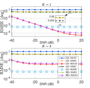
(a) Angle

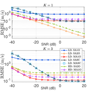
(b) Velocity

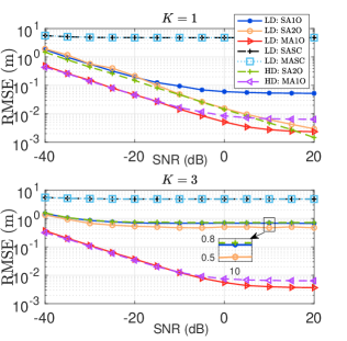
(c) Distance

Figure 4: Sensing performance versus SNR.

In Fig. 6, the impact of the beam overlap factor $\epsilon$, used to calculate the minimum number of sensing OFDM subcarriers $M$, on the RMSE of angle estimation and the feasibility probability is studied, for $\mathrm{SNR}=10$ dB and $K=1$. The feasibility probability represents the ratio of angle parameter realizations that result in successful user detection, excluding false alarms or missed detections, to all angle parameter realizations. That is, we categorize the case, where only one angle is detected, as sucessfull in the considered single-user scenario. The corresponding values of the $\epsilon$-beamwidth, $\triangle\psi_{\epsilon}$, and $M$ are provided in Table II. Fig. 6(a) shows that the RMSE increases with $\epsilon$ for all three schemes, albeit for different reasons. SA1O and SA2O rely on an angle grid where the resolution is determined by the number of subcarriers, $M$. For example, the angle resolution for $\epsilon=0.1$ is $180{{}^{\circ}}/1439=0.125{{}^{\circ}}$, resulting in an angle estimation accuracy of $0.02{{}^{\circ}}$, c.f. Fig. 6(a). In contrast, $\epsilon=0.7$ yields an angle resolution of $180{{}^{\circ}}/452=0.398{{}^{\circ}}$, leading to angle estimation accuracies of $0.13{{}^{\circ}}$ for SA1O and $0.08{{}^{\circ}}$ for SA2O, respectively, c.f. Fig. 6(a). SA2O benefits from exploiting two OFDM symbols, which provides an increased number of measurements for angle estimation, enhancing accuracy compared to SA1O. MA1O employs the high-precision ANM method, where angle resolution is unaffected by the number of subcarriers. However, a greater beam overlap, as enforced by smaller $\epsilon$, enhances the number of subcarriers effectively reflected by the user, thus providing more precise measurements for high-accuracy angle estimation. Additionally, Fig. 6(b) shows that the feasibility probabilities of SA1O and SA2O decline when $\epsilon\geq 0.5$, indicating more frequent occurrences of false alarms or missed detections. Therefore, to ensure reliable detection performance, the beam overlap factor should not exceed $\epsilon=0.5$, corresponding to the 3dB beamwidth.

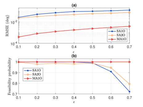
Figure 5: Sensing performance versus overlap factor of rainbow beams.

Figure 6: Achievable rate versus time for linear movement trajectory scenario with velocities of {45, 50, 55} m/s.

TABLE II: Parameters used in Figure 6.

$\epsilon$	0.1	0.2	0.3	0.4	0.5	0.6	0.7
$\frac{N_{t}}{2\pi}\triangle\psi_{\epsilon}$	0.3561	0.5151	0.6467	0.7677	0.8860	1.0066	1.1359
$M$	1439	995	793	668	579	510	452

V-B Rainbow Beam User Tracking and Communication

In this subsection, the user tracking performance is evaluated based on the achievable rate for communication, leading to optimization problem

$$\max_{{\bf w}_{k,q}}\frac{1}{Q}\sum_{q=1}^{Q}R_{k,q},\>\textrm{s.t. }|[{\bf w}_{k,q}]_{n}|=1,1\leq n\leq N_{t}.$$ (44)

Algorithms for optimization of ${\bf w}_{k,q}$ based on perfect CSI and based on the estimated direction parameters of LoS can be found in Appendix A. According to the 5G frame structure [18], the duration of one radio frame is 10 ms. For a subcarrier spacing of 120 kHz, the duration of an OFDM symbol including the CP is 8.92 $\mu$s, and the duration of a slot containing 14 OFDM symbols is 0.125 ms. In the following, the angles of the users are estimated every 10 ms. For simplicity, the number of subcarriers used for tracking of one user is set to $|\mathcal{M}_{k}|=21$ for all velocities. The sensing and communication SNRs are set to 0 dB, when the communication SNR is defined as $\mathrm{SNR}=P_{{\rm c}}\min_{\forall k}\{|\alpha_{k,0}|^{2}\}/\sigma_{\mathrm{c}}^{2}$, where $P_{{\rm c}}$ and $\sigma_{\mathrm{c}}^{2}$ are the TX power and the noise power at the users, respectively, and $|\alpha_{k,0}|^{2}=\frac{\lambda_{\mathrm{c}}^{2}}{(4\pi)^{2}D_{k}^{2}}$. The achievable rate obtained based on perfect CSI is regarded as a performance upper bound and denoted by ‘Perfect CSI’.

First, for linear motion trajectory scenarios, we study the tracking capabilities of the proposed scheme, focusing on a scenario involving three users moving on a highway. Their velocities are {45, 50, 55} m/s, and their initial positions are specified by distances {370, 448, 600} m and angles {$45{{}^{\circ}}$, $27{{}^{\circ}}$, $40{{}^{\circ}}$}. In Fig. 6(a), we compare the performances achieved with precoders designed based on the estimated LoS angles and the perfect full CSI for various Rice factors. The achievable rate is calculated every 10 ms based on the newly updated angles. Notably, for Rice factor $\rho\rightarrow\infty$, the communication performance achieved with MA1O-based tracking closely matches for perfect CSI, while SA2O exhibits a noticeable rate loss compared to the perfect CSI case, with the largest loss in achievable rate reaching approximately 0.15 bps/Hz. For Rice factors of $\rho=9$ and $\rho=4$, MA1O-based tracking introduces a small rate loss. In contrast, the rate loss for SA2O-based tracking nearly doubles to approximately 0.3 bps/Hz. In Fig. 6(b), the achievable rate, calculated for each OFDM symbol, is depicted exemplarily for $\rho\rightarrow\infty$. During the final few OFDM symbols of each radio frame, the users are tracked, and the updated CSI of LoS path are employed for communication beamforming design in the next radio frame. It is observed that with MA1O-based tracking, the initial OFDM symbols within each radio frame achieve excellent transmission rate since the LoS angles are accurately updated. However, the transmission rate gradually decreases for subsequent OFDM symbols within the same radio frame as the CSI information becomes outdated. The achievable rate of SA2O does not increase in every radio frame. We thinks this might be because the rate loss resulting from angle estimation errors could outweigh the impact of outdated angle information in certain radio frames.

Next, in Fig. 8, we investigate the achievable rate calculated at every slot for a scenario with ultra-high velocities, such as civil planes with velocities of {200, 220, 250} m/s. It is observed that both considered tracking schemes achieve nearly precise angle updates within a single radio frame, facilitating high communication rates at the start of almost each radio frame. However, given the exceptionally high user velocities, the angle information becomes quickly outdated. To ensure dependable communication services for ultra-high-velocity users, one potential strategy is to increase the tracking frequency or employ beam prediction techniques [31].

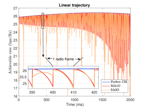
Figure 7: Achievable rate versus time for linear movement trajectory scenario with ultra-high velocities of {200, 220, 250} m/s, where $\rho\rightarrow\infty$.

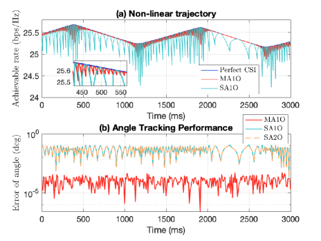
Figure 8: Achievable rate versus time for nonlinear movement trajectory scenario with velocity 15 m/s, where $\rho\rightarrow\infty$.

Finally, in Fig. 8, we study the tracking capability for a nonlinear movement trajectory scenario, where a single user with a velocity of 15 m/s is moving along a serpentine path, resulting in a non-monotonic achievable rate as a function of time, as shown in Fig. 8(a) where the achievable rate is calculated every slot. Since SA1O and SA2O achieve similar performance, hence, only the results for SA1O are presented. MA1O-based tracking consistently provides high communication rates, with negligible rate loss for most of the tracking duration. However, the rate loss becomes more pronounced, when the user transitions through the trajectory’s inflection points, leading to larger angle variations. In contrast, SA1O-based tracking typically exhibits rate losses of approximately 0.5 bps/Hz, which indcates suboptimal performance for nonlinear trajectory scenarios. Nevertheless, continuous tracking of the mobile user is still maintained. From Fig. 8(b), we deduce that the excellent rate performance of MA1O can be attributed to its ability to provide angle estimates with a precision in the range of $10^{-5}\sim 10^{-4}$, whereas SA1O yields less precise angle estimates, typically in the range of $10^{-2}\sim 10^{-1}$.

VI Conclusions

In this work, we have proposed the application of rainbow beams for ISAC in a mmWave system. OFDM radar is employed to create frequency-dependent rainbow beams based on one OFDM symbol, covering the entire angular space for fast initial access. For low-velocity users, a resource-efficient scheme based on a single-antenna radar receiver and one set of rainbow brams was proposed for estimation of the user parameters. To address the Doppler ambiguity caused by high-velocity users, two enhanced estimation schemes exploiting respectively two sets of rainbow beams and a multi-antenna radar receiver have been introduced. Furthermore, a user tracking scheme avoiding switching of PSs and TTDs has been proposed by selectively manipulating a subset of subcarriers from the radar rainbow beam, reducing the demands on control circuitry and minimizing time overhead. Our simulation results indicate that a 3 dB-beamwidth overlap is sufficient to design effective rainbow beams for sensing with a feasibility probability approaching 1. Moreover, the proposed estimation scheme based on a multi-antenna radar receiver yields high-precision estimates for the angles, distances, and velocities of the users at medium and high SNRs, realizing excellent mobile data rate performance approaching that for perfect CSI.

Appendix A Optimization of Achievable Rate for Communication

We consider a simple communication scenario to demonstrate the mitigation of the beam squint for communication and the utilization of the user parameters obtained during sensing in the proposed ISAC framework.

Denote by $\mathbf{t}_{k,q}^{{\rm com}}=[e^{-j2\pi f_{k,q}^{\rm com}\kappa_{k,1}},e^{-j2\pi f_{k,q}^{\rm com}\kappa_{k,2}},\ldots,e^{-j2\pi f_{k,q}^{\rm com}\kappa_{k,N_{t}}}]^{\mathrm{T}}$ the TTD vector for the $k$-th user on the $q$-th subcarrier. Define delay vector $\bm{\kappa}_{k}=[\kappa_{k,1},...,\kappa_{k,N_{t}}]^{{\rm T}}$, where each element is limited to $\kappa_{k,n}\in[0,1]/{f_{k,q}^{\rm com}},1\leq q\leq Q$, leading to the constraint $\kappa_{k,n}\in[0,1]/{f_{k,Q}^{\rm com}}$. The aim of designing precoding vector $\mathbf{w}_{k,q}={\bf w}_{\mathrm{PS},k}\odot\mathbf{t}_{k,q}^{{\rm com}}$ is to maximize the average rate over all the subcarriers allocated to the $k$-th user, leading to optimization problem

$$\max_{{\bf w}_{\mathrm{PS},k},\bm{\kappa}_{k}}\frac{1}{Q}\sum_{q=1}^{Q}R_{k,q},\>\textrm{s.t. }|[{\bf w}_{\mathrm{PS},k}]_{n}|=1,\kappa_{k,n}\in[0,1]/{f_{k,Q}^{\rm com}},1\leq n\leq N_{t}.$$ (45)

Using Jensen’s inequality, an upper-bound for the objective function in (45) is derived as $\frac{1}{Q}\sum_{q=1}^{Q}R_{k,q}\leq\log_{2}\left(\frac{1}{Q}\sum_{q=1}^{Q}\left(1+\frac{P_{{\rm c},k}}{\sigma_{{\rm c},k}^{2}}|\mathbf{h}_{k,q}^{\mathrm{H}}{\bf w}_{k,q}|^{2}\right)\right)$ [32, Equ. (17)]. Since the main focus of this paper is the proposed rainbow beam based training and tracking, we simplify Problem (45) by optimizing the upper-bound on the average rate. This lead to the following optimization problem,

$$\max_{{\bf w}_{\mathrm{PS},k},\bm{\kappa}_{k}}\sum_{q=1}^{Q}|\mathbf{h}_{k,q}^{\mathrm{H}}{\bf w}_{k,q}|^{2},\>\textrm{s.t. }|[{\bf w}_{\mathrm{PS},k}]_{n}|=1,\kappa_{k,n}\in[0,1]/{f_{k,Q}^{\rm com}},1\leq n\leq N_{t},$$ (46)

where $|\mathbf{h}_{k,q}^{\mathrm{H}}{\bf w}_{k,q}|^{2}={\bf w}_{\mathrm{PS},k}^{{\rm H}}{\rm diag}((\mathbf{t}_{k,q}^{{\rm com}})^{{\rm H}})\mathbf{h}_{k,q}\mathbf{h}_{k,q}^{\mathrm{H}}{\rm diag}(\mathbf{t}_{k,q}^{{\rm com}}){\bf w}_{\mathrm{PS},k}$.

We firsty assume that the full CSI for $\text{$\mathbf{h}$}_{k,q}$ is available. Given delay vector $\bm{\kappa}_{k}$, the optimal ${\bf w}_{\mathrm{PS},k}$ for Problem (46) is given by ${\bf w}_{\mathrm{PS},k}^{\mathrm{opt}}=\exp\left\{j\angle\mathbf{u}_{k}\right\}$, where $\mathbf{u}_{k}$ is the eigenvector corresponding to the largest eigenvalue of matrix $\sum_{q=1}^{Q}{\rm diag}((\mathbf{t}_{k,q}^{{\rm com}})^{{\rm H}})\mathbf{h}_{k,q}\mathbf{h}_{k,q}^{\mathrm{H}}{\rm diag}(\mathbf{t}_{k,q}^{{\rm com}})$ and $\exp\left\{j\angle\left(\cdot\right)\right\}$ is an element-wise operation. Given ${\bf w}_{\mathrm{PS},k}$, the optimal $\mathbf{t}_{k,q}^{{\rm com}}$ is obtained as $(\mathbf{t}_{k,q}^{{\rm com}})^{\rm opt}=\exp\left\{j\angle\left({\rm diag}({\bf w}_{\mathrm{PS},k}^{{\rm H}})\mathbf{h}_{k,q}\right)\right\}$ if we ignore the dependence of $\bm{\kappa}_{k}$ for the moment. Then, the optimal delay $\bm{\kappa}_{k}$ should satisfy

$$\min_{\bm{\kappa}_{k}}\sum_{q=1}^{Q}\left\|\bm{\kappa}_{k}+\frac{1}{2\pi f_{k,q}^{\rm com}}\angle\left((\mathbf{t}_{k,q}^{{\rm com}})^{\rm opt}\right)\right\|_{2}^{2},\>\textrm{s.t. }\kappa_{n}\in[0,1]/{f_{k,Q}^{\rm com}},1\leq n\leq N_{t},$$ (47)

and is given by $\bm{\kappa}_{k}^{{\rm opt}}=-\frac{1}{Q}\sum_{q=1}^{Q}\left(\frac{1}{2\pi f_{k,q}^{\rm com}}\angle\left({\rm diag}({\bf w}_{\mathrm{PS},k}^{{\rm H}})\mathbf{h}_{k,q}\right)\right)$. Finally, ${\bf w}_{\mathrm{PS},k}^{\mathrm{opt}}$ and $\bm{\kappa}_{k}^{{\rm opt}}$ are updated iteratively.

However, when only the CSI of the LoS path is available in terms of AoDs and propagation delays, as obtained via user training and tracking, the suboptimal problem corresponding to Problem (46) is given by

$$\max_{{\bf w}_{\mathrm{PS},k},\bm{\kappa}_{k}} \sum_{q=1}^{Q}{\bf w}_{k,q}^{\mathrm{H}}\mathbf{a}_{N_{t}}\left(\theta_{k},f_{{\rm c}}+f_{k,q}^{\rm com}\right)\mathbf{a}_{N_{t}}^{\mathrm{H}}\left(\theta_{k},f_{{\rm c}}+f_{k,q}^{\rm com}\right){\bf w}_{k,q},$$

s.t. $$|[{\bf w}_{\mathrm{PS},k}]_{n}|=1,\kappa_{n}\in[0,1]/{f_{k,Q}^{\rm com}},1\leq n\leq N_{t}.$$ (48)

According to Section (II-B1), the optimal delay vector is given by $\bm{\kappa}_{k}^{{\rm opt}}=\frac{d}{c}\cos\theta_{k}[0,1,...,N_{t}-1]^{{\rm T}}$, and the optimal phase shift vector is given by ${\bf w}_{\mathrm{PS},k}^{\mathrm{opt}}=\mathbf{a}_{N_{t}}\left(\theta_{k},f_{{\rm c}}\right)$.

References

- [1] C. Sturm and W. Wiesbeck, “Waveform design and signal processing aspects for fusion of wireless communications and radar sensing,” Proc. IEEE, vol. 99, no. 7, pp. 1236–1259, Jul. 2011.
- [2] F. Liu, Y. Cui, C. Masouros et al., “Integrated sensing and communications: Toward dual-functional wireless networks for 6G and beyond,” IEEE J. Sel. Areas Commun., vol. 40, no. 6, pp. 1728–1767, Jun. 2022.
- [3] J. A. Zhang, F. Liu, C. Masouros et al., “An overview of signal processing techniques for joint communication and radar sensing,” IEEE J. Sel. Topics Signal Process., vol. 15, no. 6, pp. 1295–1315, Nov. 2021.
- [4] Y. Zeng and X. Xu, “Toward environment-aware 6G communications via channel knowledge map,” IEEE Wireless Commun., vol. 28, no. 3, pp. 84–91, Jun. 2021.
- [5] K. Hosoya et al., “Multiple sector ID capture (MIDC): A novel beamforming technique for 60-GHz band multi-gbps WLAN/PAN systems,” IEEE Trans. Antennas Propag., vol. 63, no. 1, pp. 81–96, Jan. 2015.
- [6] Z. Xiao, T. He, P. Xia, and X.-G. Xia, “Hierarchical codebook design for beamforming training in millimeter-wave communication,” IEEE Trans. Wireless Commun., vol. 15, no. 5, pp. 3380–3392, May 2016.
- [7] A. Ali, N. Gonzalez-Prelcic, and R. W. Heath, “Millimeter wave beam selection using out-of-band spatial information,” IEEE Trans. Wireless Commun., vol. 17, no. 2, pp. 1038–1052, Feb. 2018.
- [8] V. Desai et al., “Initial beamforming for mmWave communications,” in Proc. 48rd Asilomar Conf. Signals, Syst., Comput., Nov. 2014, pp. 1926–1930.
- [9] C. N. Barati et al., “Initial access in millimeter wave cellular systems,” IEEE Trans. Wireless Commun., vol. 15, no. 12, pp. 7926–7940, Dec. 2016.
- [10] S. Kalia, S. A. Patnaik, B. Sadhu, M. Sturm, M. Elbadry, and R. Harjani, “Multi-beam spatio-spectral beamforming receiver for wideband phasedarrays,” IEEE Trans. Circuits Syst. I, vol. 60, no. 8, pp. 2018–2029, Aug. 2013.
- [11] C.-C. Lin et al., “Wideband beamforming with rainbow beam training using reconfigurable true-time-delay arrays for millimeter-wave wireless [feature],” IEEE Circuits Syst. Mag., vol. 22, no. 4, pp. 6–25, Fourthquarter 2022.
- [12] H. Yan, V. Boljanovic, and D. Cabric, “Wideband millimeter-wave beam training with true-time-delay array architecture,” in Proc. 53rd Asilomar Conf. Signals, Syst., Comput., Nov. 2019, pp. 1447–1452.
- [13] V. Boljanovic, H. Yan, C.-C. Lin, S. Mohapatra, D. Heo, S. Gupta, and D. Cabric, “Fast beam training with true-time-delay arrays in wideband millimeter-wave systems,” IEEE Trans. Circuits Syst. I, vol. 68, no. 4, pp. 1727–1739, Apr. 2021.
- [14] J. Tan and L. Dai, “Wideband beam tracking in THz massive MIMO systems,” IEEE J. Sel. Areas Commun., vol. 39, no. 6, pp. 1693–1710, Jun. 2021.
- [15] M. Cui, L. Dai, Z. Wang, S. Zhou, and N. Ge, “Near-field rainbow: Wideband beam training for XL-MIMO,” IEEE Trans. Wireless Commun., vol. 22, no. 6, pp. 3899–3912, Jun. 2023.
- [16] H. Luo, F. Gao, W. Yuan, and S. Zhang, “Beam squint assisted user localization in near-field integrated sensing and communications systems,” IEEE Trans. Wireless Commun., pp. 1–1, 2023, Early Access.
- [17] H. Luo, F. Gao, H. Lin, S. Ma, and H. V. Poor, “YOLO: An efficient terahertz band integrated sensing and communications scheme with beam squint,” 2023. [Online]. Available: https://arxiv.org/abs/2305.12064
- [18] NR; Physical channels and modulation (Release 18). document TS 38.211 V18.0.0, Technical Specifications Group RadioAccess Network, 3GPP, Dec. 2023.
- [19] Y. S. Cho, J. Kim, W. Y. Yang, and C. G. Kang, MIMO-OFDM WIRELESS COMMUNICATIONS WITH MATLAB. Wiley Publishing, 2010.
- [20] NR; Base Station (BS) Radio Transmission and Reception Release 15. Document TS 38.104 v15.4.0, Technical Specifications Group RadioAccess Network, 3GPP, Dec. 2018.
- [21] Evolved Universal Terrestrial Radio Access (E-UTRA); Base Station (BS) Radio Transmission and Reception Release 15. document TS 36.104 v15.3.0, Technical Specifications Group RadioAccess Network, 3GPP, Jun. 2018.
- [22] B. Ning, Z. Chen, Z. Tian, C. Han, and S. Li, “A unified 3D beam training and tracking procedure for terahertz communication,” IEEE Trans. Wireless Commun., vol. 21, no. 4, pp. 2445–2461, Apr. 2022.
- [23] F. Liu, W. Yuan, C. Masouros, and J. Yuan, “Radar-assisted predictive beamforming for vehicular links: Communication served by sensing,” IEEE Trans. Wireless Commun., vol. 19, no. 11, pp. 7704–7719, Aug. 2020.
- [24] F. Liu, Y.-F. Liu, A. Li, C. Masouros, and Y. C. Eldar, “Cramér-rao bound optimization for joint radar-communication beamforming,” IEEE Trans. Signal Process., vol. 70, pp. 240–253, Dec. 2022.
- [25] S. J. Orfinidas, “Electromagnetic waves and antennas,” Aug. 2016. [Online]. Available: https://www.ece.rutgers.edu/ orfanidi/ewa/
- [26] G. Hakobyan and B. Yang, “A novel intercarrier-interference free signal processing scheme for OFDM radar,” IEEE Trans. Veh. Technol., vol. 67, no. 6, pp. 5158–5167, Jun. 2018.
- [27] A. L. Swindlehurst, G. Zhou, R. Liu, C. Pan, and M. Li, “Channel estimation with reconfigurable intelligent surfaces-a general framework,” Proc. IEEE, vol. 110, no. 9, pp. 1312–1338, Sept. 2022.
- [28] J. Tropp, “Greed is good: Algorithmic results for sparse approximation,” IEEE Trans. Inf. Theory, vol. 50, no. 10, pp. 2231–2242, Oct. 2004.
- [29] A. J. Barabell, “Improving the resolution performance of eigenstructure-based direction-finding algorithms,” in Proc. IEEE Intl. Conf. Acoust. Speech Signal, vol. 8, Apr. 1983, pp. 336–339.
- [30] B. N. Bhaskar, G. Tang, and B. Recht, “Atomic norm denoising with applications to line spectral estimation,” IEEE Trans. Signal Process., vol. 61, no. 23, pp. 5987–5999, Dec. 2013.
- [31] M. Garkisch, S. Lotter, G. Zhou, V. Jamali, and R. Schober, “User tracking and direction estimation codebook design for IRS-assisted mmwave communication,” Mar. 2024. [Online]. Available: https://arxiv.org/abs/2403.06818
- [32] F. Sohrabi and W. Yu, “Hybrid analog and digital beamforming for mmwave ofdm large-scale antenna arrays,” IEEE Journal on Selected Areas in Communications, vol. 35, no. 7, pp. 1432–1443, Jul. 2017.