Hydrodynamic behavior near dynamical criticality
of a facilitated conservative lattice gas
Abstract
We investigate a -conservative lattice gas exhibiting a dynamical active-absorbing phase transition with critical density . We derive the hydrodynamic equation for this model, showing that all critical exponents governing the large scale behavior near criticality can be obtained from two independent ones. We show that as the supercritical density approaches criticality, distinct length scales naturally appear. Remarkably, this behavior is different from the subcritical one. Numerical simulations support the critical relations and the scale separation.
Models displaying dynamical phase transitions have attracted increasing scrutiny in recent years. Such models are tightly related to self-organizing criticality: open systems dynamically adjust their density in order to reach a critical state at density , often displaying non-trivial scaling properties. This phenomenon manifests itself, in a closed system, as a dynamical phase transition: below , the system reaches an absorbing state, while above , it remains in a quasi-stationary active state.
A fundamental example of such a model is the constrained conservative lattice gas (CLG) [1], also referred to as facilitated exclusion process in the recent literature. It is defined as an exclusion particle system (i.e. any system site cannot contain more than one particle) on a -dimensional lattice, where so-called active particles jump randomly at rate to each empty nearest neighbor111Sometimes, simultaneous jumps are considered [1], but this does not change the critical behavior of the model.. A particle is considered active if at least one of its neighboring sites is also occupied, and the total number of particles is conserved. Related models featuring an absorbing phase transition have generated an intense research activity, like for instance the paradigm Manna sandpile model [3, 4, 5, 6]. In particular many of these models, including the CLG, exhibit a hyperuniform critical state [7, 8], for which we still have a limited knowledge. The CLG has been investigated numerically in [1, 9, 7, 8] when and theoretically in [10, 11, 12, 13, 14, 15, 16] when . We focus here on the -dimensional case, and recall some previous results already obtained in the -dimensional case.
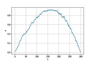
Clearly, this system remains active whenever , and could reach an absorbing state whenever . It appears, however, that in dimension , the dynamical critical density is strictly smaller than . That is, in the regime , even though an absorbing state will be ultimately reached in any finite system, on physically relevant timescales a quasi-stationary active state is observed. In order to illustrate this phenomenon, the average absorption time is numerically represented in Fig. 1 in both subcritical and supercritical regimes.
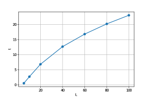
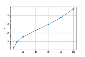
The CLG is reflection symmetric and isotropic, and therefore its macroscopic density profile , taken in the diffusive space-time scaling limit, is expected to be a solution to the parabolic equation with scalar diffusion coefficient . In the subcritical regime the particles become blocked in subdiffusive time scales (see Fig. 1a), therefore . When the initial profile has both subcritical and supercritical regions, the supercritical phase progressively invades the subcritical “frozen” areas. That is, one should interpret the above hydrodynamic equation as a Stefan problem. In dimension this result is established mathematically in [14], and exploits the explicit expression of the stationary states, a feature that is lost in higher dimensions.
In this letter we explore the scaling properties of the two-dimensional model, with a particular focus on the active phase. We study the critical exponents for all relevant macroscopic quantities, both theoretically and numerically, as it has been done for other models, for instance in [17]. We are able to deduce relationships between those critical exponents, which are of independent interest, and check them by simulations.
Macroscopic observables. Of particular interest are the critical and near criticality behavior of the model. It has been noted in [7] that the CLG could have two separate length scales near criticality. While in their simulations these two scales seem to coincide, we will see here that in the supercritical phase they differ. Let us define:
-
•
The geometric correlation length : this is the scale which is mostly used in the literature [18, Section 3.3], and is the one discussed in [1]. It describes the spread of activity. More precisely, to sustain activity, particle clusters must self-activate, i.e., a particle activates its neighbor, which further activates its neighbors, until closing a cycle and re-activating the particle we started with. The diameter of this self-activated structure is described by the geometric correlation length .
This means that, for a finite system of size , if , then there is no quasi-stationary state, and in that case activity will decay until dying out. On the other hand, if , then the activity behaves in the same manner as .
- •
Both length scales diverge when approaching criticality, as and , for some critical exponents and , which we now investigate.
In [1, 7], several other critical exponents are determined. Notably, in the latter the authors show that the CLG’s absorbing state is hyperuniform, i.e. the number of particles in a ball or radius has standard deviations of order , for smaller than .
We are interested in the hydrodynamic behavior of the CLG, whose diffusion coefficient behaves, close to , as for some exponent . In order to understand the noise’s amplitude, we also consider the compressibility . For the CLG, the dominant parameter for the system is the density of active particles, . However, the notion of active particles is in fact ambiguous, since one may or may not count as active particles who are fully surrounded by other particles (and therefore cannot move). For this reason, we distinguish between , the density of particles having at least one occupied neighbor (which is the one considered in [1]), and the activity , which counts the local number of possible jumps. We will see further that in fact both exponents and coincide (Fig. 3). This means that the perimeter of clusters of active particles is of the same order as their volume.
Relations between critical exponents. By numerical simulations we are able to get all the critical exponents in the case . In dimension , we have exact values, as discussed below.
A number of relations can be derived between the relevant critical exponents [18]. Most of them are standard, a detailed derivation will be given in a companion article [21]. The first one ties the compressibility to the particle fluctuations and the activity correlation length, as
| (1) |
This relation can be obtained by considering the structure factor (see [22, Section II.2.1]), which encapsulates the -point statistics of the distribution at a fixed time [19]. By the scaling hypothesis, can only depend on via the combination . Moreover, , and at criticality when is small. These three facts impose the form
| (2) |
and hence remains of order as . This implies equation (1).
A similar scaling relation can be obtained for the geometric correlation length. Indeed, at scales smaller than the system looks critical, so that the critical density fluctuations are larger than , and “hide” the off-criticality. The scale is therefore characterized by the relation . This yields the following relation:
| (3) |
The next relation stems from Einstein’s relation and the fact that the noise amplitude is determined by the number of possible particle jumps (see [22, Section II.2] for instance): this leads to
| (4) |
Finally, the following relation is a consequence of a particular property of the CLG, called gradient condition [23, 22], which relies on well-chosen jump rates for the system. Under this condition,
| (5) |
where (resp. ) denotes the average number of particles (resp. active particles) at site . At the macroscopic level, this identity translates as
| (6) |
and yields in turn that . Near criticality, this implies
| (7) |
Note that equations (4) and (7) give As an interesting consequence, the fact that , i.e. that clusters of active particles have volume and perimeter of the same order, implies . In Table I we give all exponents in both and cases. The former are exact values, while the latter are numerically computed.
Hydrodynamics and scale invariance. Near criticality, we are interested in the macroscopic evolution of . It evolves according to the fluctuating hydrodynamic equation
| (8) |
The noise depends on the scale at which we look: at distances above correlations are small and is white noise, while for distances smaller than the noise will have non-trivial correlations:
| (9) |
for some exponent . In the regime below , the density fluctuations are proportional to , hence equation (8) must be invariant under the parameter rescaling
| (10) |
This forces to be equal , and
| (11) |
We emphasize that on a length above the scale invariance is not the same, and in particular the dynamic exponent will change. This scale separation has been noted qualitatively in [1].
| obs. | ||||||||
|---|---|---|---|---|---|---|---|---|
| exp. | ||||||||
| -0.38 | 1 and 1.07 | 0.77 | 1.8 | 0.70 | 0.62 | 0.62 | 1.51 | |
| 0.78222obtained in [1] | 0.775333obtained in [7] | 0.632 | 1.522 |
One-dimensional case. The one-dimensional case has been recently under scrutiny, and its macroscopic evolution is now quite well understood. It has been proved rigorously [14, 13] that the critical density is given by , and the diffusive supercritical phase progressively invades the subcritical phase via flat interfaces, until either one of the phases disappears. In this respect, a crucial feature of the one-dimensional case lies in its explicit supercritical grand canonical states either parametrized by the density or the active density . These grand canonical states can be defined sequentially, by filling an arbitrary site with probability , and then following each empty site by a particle with probability , but each particle by another particle with probability .
Precisely, the hydrodynamic limit in is given by , with diffusion coefficient
| (12) |
and critical exponent . The explicit construction of the grand-canonical state yields the other observables for , as well as their critical exponent (see [15]): namely the activity with , and the compressibility , with Moreover, the stationary measure can be seen as a nearest-neighbor spin system with chemical potential , and an interaction which gives infinite costs to two neighboring empty sites. This can be solved using standard methods involving the transfer matrix (see [24, Chapter 6]), which here is given by
All the relevant quantities and exponents for the one-dimensional model are listed in Table I.
Numerical simulations. We note that in finite systems the critical density depends slightly on the geometry, so that in the analysis of the simulated data we do not enforce a single critical density for systems of different sizes or boundary conditions.
In order to numerically derive the diffusion coefficient and verify relation (7), we simulate a cylindrical system, i.e. periodic in the vertical direction, of size put in contact at the left and right boundaries with particle reservoirs with respective densities and . More specifically, at the boundary, particles are removed at rate , , and empty sites are filled at rate , . In our simulations, boundary particles are always considered active.
When the system reaches a quasi-stationary state with density . For our particular choice of boundary interactions, meaning that the reservoirs enforce the density of active particles and not the total density of particles. This relation is, however, not universal, and depends on the exact boundary dynamics considered.
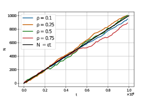
In order to estimate the diffusion coefficient, we fix and with small . We measure the total net number of particles crossing the system up to time . In general, we expect the current to be proportional to
| (13) |
where . Since our system is gradient and for our specific choice of reservoirs, we should obtain . which is verified by our simulation, see Fig. 2. In particular this shows that .
In more general models (for instance when the gradient property is not satisfied) we do not necessarily expect to be constant, but still of order (namely, neither diverging nor decaying as ).
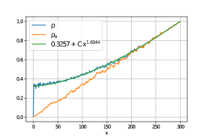
The scaling exponents and can be found by simulating the system with cylindrical geometry, maintaining one reservoir at density and the other one at density . We then measure, at each section of the cylinder, , and . See Fig. 3.
Thanks to the gradient property of the model and our choice of reservoirs, grows linearly with the horizontal distance, from at to at . This is verified in our simulation (Fig. 3a). Thanks to this result, the relation can then be written as . By fitting in Fig. 3a we obtain . Finally, noting that for small the activity is linear in (Fig. 3b), we conclude .
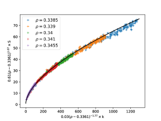
In order to find the remaining exponents, we estimate the structure factor for different values of . This is done on a system with periodic boundaries (in both directions). By fitting the data to equation (2), posing and , we obtain the values in Table I. See Fig. 4.
All the simulations used in this article are open access, available at https://github.com/alexandreroget/2D_FacilitatedExclusionProcess.
Conclusion. In this article, we discussed the critical scaling for the CLG. We saw that there are three independent critical exponents, , , and , that all other exponents () could be deduced from. Due to repulsion, active cluster sizes are of order , so their perimeter is proportional to the volume, thus and all scaling is described by two independent exponents.
We numerically computed several critical exponents for the –CLG (see Table 1), and confronted them both with those critical relations, and the numerical values in [1] and [7] for CLG with simultaneous jumps. We obtained very good agreement between them; with the exception of and . While our numerical values fit the theoretical relations introduced above, they are different from those of [7]. The reason seems to be that we approach the critical state from , while [7] do from . Recently, [8] went further investigating the approach to hyperuniformity from the subcritical regime; on the contrary to [7], they find that the critical exponent (which they denote ) is different from .
We emphasize the existence of two distinct correlation lengths, one characterizing the size of self-activating clusters, and the other one characterizing the two-points correlation decay. This distinction is a specific feature of the quasi-stationary regime , and for this reason does not exist in one dimension. We conjecture that it is a common feature of any dimension , because the rigid structure necessary to reach a frozen state at density results in the quasi-stationary regime.
Unlike in the one-dimensional case, the diffusion coefficient has negative exponent (see Table 1), and is therefore discontinuous at . We note that the diffusion term operating in the supercritical phase instantly creates at the boundary non-zero density gradients. Therefore, this discontinuity does not create a quantitative different behavior than the –Stefan problem, which has a finite critical diffusion coefficient (12). That is, subcritical regions are frozen while particles in supercritical regions diffuse; and the interfaces between them move as the supercritical regions invade the subcritical ones. The divergence of is balanced out by small non-zero density gradients, resulting in a finite current. Hence, as in dimension one, the interfaces move with finite speed.
Acknowledgements.
This project is partially supported by the ANR grant MICMOV (ANR-19-CE40-0012) of the French National Research Agency (ANR). It has received funding from the European Research Council (ERC) under the European Union’s Horizon 2020 research and innovative program (grant agreement n° 715734), and from Labex CEMPI (ANR-11-LABX-0007-01).References
- Rossi et al. [2000] M. Rossi, R. Pastor-Satorras, and A. Vespignani, Universality class of absorbing phase transitions with a conserved field, Phys. Rev. Lett. 85, 1803 (2000).
- Note [1] Sometimes, simultaneous jumps are considered [1], but this does not change the critical behavior of the model.
- Manna [1991] S. S. Manna, Two-state model of self-organized criticality, Journal of Physics A: Mathematical and General 24, L363 (1991).
- Dickman et al. [2001] R. Dickman, M. Alava, M. A. Muñoz, J. Peltola, A. Vespignani, and S. Zapperi, Critical behavior of a one-dimensional fixed-energy stochastic sandpile, Phys. Rev. E 64, 056104 (2001).
- Mukherjee and Pradhan [2023] A. Mukherjee and P. Pradhan, Dynamic correlations in the conserved manna sandpile, Phys. Rev. E 107, 024109 (2023).
- Tapader et al. [2021] D. Tapader, P. Pradhan, and D. Dhar, Density relaxation in conserved manna sandpiles, Phys. Rev. E 103, 032122 (2021).
- Hexner and Levine [2015] D. Hexner and D. Levine, Hyperuniformity of critical absorbing states, Phys. Rev. Lett. 114, 110602 (2015).
- Goldstein et al. [2024] S. Goldstein, J. L. Lebowitz, and E. R. Speer, Approach to hyperuniformity of steady states of facilitated exchange processes, arXiv:2401.16505 (2024).
- Lübeck [2001] S. Lübeck, Scaling behavior of the absorbing phase transition in a conserved lattice gas around the upper critical dimension, Phys. Rev. E 64, 016123 (2001).
- [10] A. Ayyer, S. Goldstein, J. L. Lebowitz, and E. R. Speer, Stationary states of the one-dimensional facilitated asymmetric exclusion process, arXiv:2010.07257 .
- Goldstein et al. [2019] S. Goldstein, J. L. Lebowitz, and E. R. Speer, Exact solution of the facilitated totally asymmetric simple exclusion process, Journal of Statistical Mechanics: Theory and Experiment 2019, 123202 (2019).
- [12] S. Goldstein, J. L. Lebowitz, and E. R. Speer, The discrete-time facilitated totally asymmetric simple exclusion process, Pure Appl. Funct. Anal. 6.
- Blondel et al. [2020] O. Blondel, C. Erignoux, M. Sasada, and M. Simon, Hydrodynamic limit for a facilitated exclusion process, Ann. Inst. H. Poincaré Probab. Statist. 56, 667 (2020).
- Blondel et al. [2021] O. Blondel, C. Erignoux, and M. Simon, Stefan problem for a nonergodic facilitated exclusion process, Probability and Mathematical Physics 2, 127 (2021).
- Erignoux and Zhao [2023] C. Erignoux and L. Zhao, Stationary fluctuations for the facilitated exclusion process, ArXiv preprint: 2305.13853 (2023), 2305.13853 .
- Da Cunha et al. [2024] H. Da Cunha, C. Erignoux, and M. Simon, Hydrodynamic limit for a boundary-driven facilitated exclusion process, arXiv: 2401.16535 (2024).
- Chatterjee et al. [2018] S. Chatterjee, A. Das, and P. Pradhan, Hydrodynamics, density fluctuations, and universality in conserved stochastic sandpiles, Phys. Rev. E 97, 062142 (2018).
- Hinrichsen [2000] H. Hinrichsen, Non-equilibrium critical phenomena and phase transitions into absorbing states, Advances in Physics 49, 815 (2000), https://doi.org/10.1080/00018730050198152 .
- Ghosh and Lebowitz [2017] S. Ghosh and J. L. Lebowitz, Large deviations and rigidity in hyperuniform systems: A brief survey, Indian J Pure Appl Math 48, 609 (2017).
- T20 [2018] Hyperuniform states of matter, Physics Reports 745, 1 (2018).
- Erignoux et al. [2024] C. Erignoux, A. Roget, A. Shapira, and M. Simon, Work in progress, (2024+).
- Spohn [1991] H. Spohn, Large Scale Dynamics of Interacting Particles (Springer-Verlag, 1991).
- Kipnis and Landim [1999] C. Kipnis and C. Landim, Scaling limits of interacting particle systems, Grundlehren der Mathematischen Wissenschaften [Fundamental Principles of Mathematical Sciences], Vol. 320 (Springer-Verlag, Berlin, 1999) pp. xvi+442.
- Kardar [2007] M. Kardar, Statistical Physics of Particles (Cambridge: Cambridge University Press, 2007).