Anomalous quantum scattering and transport of electrons with Mexican-hat dispersion induced by electrical potential
Abstract
We theoretically study the quantum scattering and transport of electrons with Mexican-hat dispersion through both step and rectangular potential barriers by using the transfer matrix method. Owing to the torus-like iso-energy lines of the Mexican-hat dispersion, we observe the presence of double reflections and double transmissions in both two different barrier scenarios, i.e., the normal reflection (NR), retro-reflection (RR), normal transmission (NT), and specular transmission (ST). For the step potential with electrons incident from the large wavevector, the transmission is primarily governed by NT with nearly negligible ST, while the reflection is dominant by RR (NR) within (outside) the critical angle. Additionally, for electrons incident from the small wavevector, the NT can be reduced to zero by adjusting the barrier, resulting in a significant enhancement of ST and RR. For the rectangular barrier, the transmission and reflection spectra resemble those of the step barrier, but there are two kinds of resonant tunneling which can lead to perfect NT or ST. There exists a negative differential conductance (NDC) effect in the conductance spectrum. The conductance and the peak-to-valley ratio of the NDC effect can be effectively controlled by adjusting the height and width of the barrier as well as the incident energy. Our results provide a deeper understanding of the electron states governed by the Mexican-hat dispersion.
I INTRODUCTION
The discovery of graphene in 2004 marked the beginning of extensive research on two-dimensional (2D) materials Novoselov1 . Since then, 2D materials have rapidly gained prominence in condensed matter physics due to their critical dimensions, atomic thickness, and diverse band structures Sahin ; Shaoliang Yu ; Gibertini . Many excellent and exotic properties associated to 2D materials can not be found in their bulk counterparts Sahin ; Shaoliang Yu ; Gibertini ; Gao ; Hui Cai ; Tuan . To date, a considerable number of new 2D materials have been both theoretically predicted and experimentally synthesized Gao ; Hui Cai ; Tuan . The band structures of 2D materials change qualitatively as the thickness is reduced to few or monolayer. The most famous example is graphene, which has a linear dispersion near the Fermi level, requiring a description by 2D Dirac equation Novoselov . Indirect-direct band gap transition occurs when the thickness of 2D transition metal dichalcogenides (TMDCs) decreases to monolayer Mak . For some 2D materials, the band structure undergos a transformation from a parabolic dispersion into a Mexican-hat shape as their thickness decreases to monolayer, which is also known as a Lifshiftz transition Zolyomi . Several 2D electron systems possess Mexican-hat dispersion in the low energy regime, as confirmed by experiments Min ; Jiang ; Falko2016 ; Jappor ; Ariapour ; Demirci ; Bandurin ; Kibirev . Notable examples include the gated bilayer graphene Min , the inverted InAs/GaSb double quantum well Jiang , and the ultrathin 2D group IIIA metal chalcogenides MX (M=Ga, In and X=S, Se, Te) Falko2016 ; Jappor ; Ariapour ; Demirci ; Bandurin ; Kibirev . Interestingly, the Mexican-hat shaped bands can be tuned by strain or electric fields. For instance, in monolayer InSe, the brim of the Mexican-hat bands can be continuously manipulated by strain HuTing ; Zhouma1 or a vertical electric field Skinner ; XiaoXB , accompanying with an indirect-direct band gap transition.
A prominent feature of Mexican-hat-shaped bands is the singularity in the density of states at or near the band edge, where the density of modes exhibits an abrupt step function Nurhuda ; Seixas ; Cao ; Heremans ; Ghobadi ; Houssa ; Xu-Jin Ge ; Drummond ; Wickramaratne . The distorted density of states results in exotic electric and magnetic properties in electron systems with sombrero-shaped dispersion Nurhuda ; Seixas ; Cao ; Heremans ; Ghobadi ; Houssa ; Xu-Jin Ge ; Drummond ; Wickramaratne , such as the multi-ferroic effect in -SnO Seixas , tunable magnetism and half-metallicity monolayer GaSe Cao , the enhanced thermoelectric efficiency in few-layer III-VI materials Heremans ; Houssa ; Xu-Jin Ge ; Wickramaratne , and the Lifshitz transitions in 2D InSe Drummond . In addition, the interplay between the Mexican-hat dispersion and the Rashba/Dresselhaus spin-orbit coupling may result in the spin-charge conversion Zhouma2 and spin polarization Zhouma3 . In conventional semiconductors, the Fermi surface is a circle, and electron scattering against potential barrier follows a Snell’s law akin to optics Griffiths , resulting in specular reflection and normal transmission. This behavior is also observed in graphene. However, graphene p-n junctions exhibit exotic negative refraction Cheianov ; GHLee , which is useful to focus the electron beam. For electrons with Mexican-hat shaped bands, the Fermi surfaces are two concentric circles, similar to a torus. There are two extra scattering channels, which will give rise to novel scattering features when electrons encounter a potential barrier. However, this topic remains unexplored, and the underlying scattering mechanisms are exclusive.
In this work, we theoretically study the quantum scattering and transport of electrons with Mexican-hat dispersion through both step and rectangular potential barriers by using the transfer matrix method. Owing to the torus-like iso-energy lines of the Mexican-hat dispersion, we observe the presence of double reflections and double transmissions in both two different barrier scenarios, i.e., the normal reflection (NR), retro-reflection (RR), normal transmission (NT), and specular transmission (ST). For the step potential with electrons incident from the large wavevector, the transmission is primarily governed by NT with nearly negligible ST, while the reflection is dominant by RR (NR) within (outside) the critical angle. Additionally, for electrons incident from the small wavevector, the NT can be reduced to zero by adjusting the barrier, resulting in a significant enhancement of ST and RR. For the rectangular barrier, the transmission and reflection spectra resemble those of the step barrier, but there are two kinds of resonant tunneling which can lead to perfect NT or ST. There exists a negative differential conductance (NDC) effect in the conductance spectrum. The conductance and the peak-to-valley ratio of the NDC effect can be effectively controlled by adjusting the height and width of the barrier as well as the incident energy.
The rest of this paper is organized as follows. In Sec. II, the quartic model and transfer matrix method for the Mexican-hat-dispersion electrons are introduced. In Sec. III, numerical results and discussions for the scattering and transport of Mexican-hat-dispersion electrons are presented. Finally, a brief summary of the results is given in Sec. IV.
II MODEL AND METHODS
The simplest Mexican-hat dispersion takes the form of the quartic model MaZhou1
| (1) |
where and are constants meeting the conditions and for the conduction band while and for the valence band. The energy = represents the height of the Mexican hat, and k= is the wave vector. The single-particle effective Hamiltonian corresponding to Eq. 1 can be written as
| (2) |
which is obtained by replacing the wave vectors (, ) with differential operators (, ) in Eq. (1). For a fixed electron energy , we have
| (3) |
which means the iso-energy lines, i.e., the Fermi surfaces, are two concentric circles. Their radii are =with =, where indicates the small (big) iso-energy circles. The probability current density along the two direction can be obtained by , which are given by
| (4) |
Therefore, the direction of the probability current density is identical (opposite) to the direction of the wave vector on the small (big) iso-energy circle.
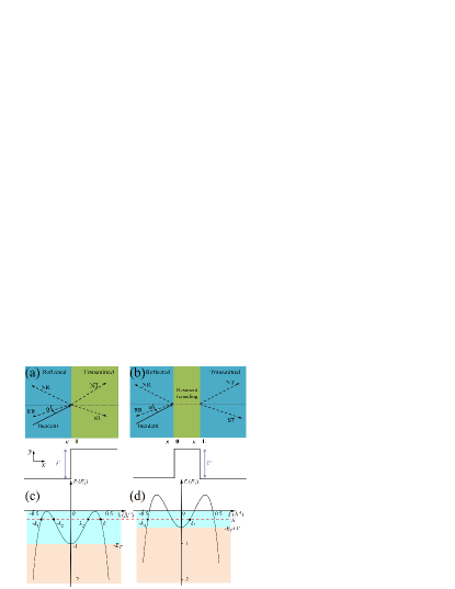
II.1 Scattering at the interface of a step potential barrier
Firstly, we consider the scattering at interface of a step potential barrier along the -direction with the height as shown in Fig. 1(a). According to the Mexican-hat dispersion shown in Fig. 1(c), we can divide the incident electron energy into two distinct regimes, each giving rise to different scattering mechanisms. The first regime is , as indicated by the light cyan region in Fig. 1(c), in which the electron energy is confined within the Mexican-hat. In this scenario, at a specific energy level, there exist four modes as shown in Fig. 1(c), two propagating forward ( and states) and two propagating backward ( and states). Consequently, one will observe retro-reflection and specular transmission, i.e., the negative refraction, in addition to the normal reflection and transmission, which is absent in the electron scattering of conventional 2D electron gas. Since there are two modes propagating forward along the -direction, we should discuss them separately. If the electron is incident with the wave vector , the wave functions in the incident/reflection () and the transmission () regions in Fig. 1(a) can be expressed respectively as
| (5) | ||||
where =. The wavevectors are =, =, , and with . We have omitted the common factor in Eq. (5) because the wavevector is conserved arising from the translation invariance along the -direction.
The type of each scattering ( and ) can be classified according to the relative orientation between the wave vector and the group velocity of both reflected and transmitted electrons. The group velocity for a given states is . We can use the product of the wave vector and the group velocity to manifest the relative orientation between them. For the reflected electron state with wave vector , we have , which is consistent with that of the incident electron state. Therefore, this is a normal reflection (NR) with magnitude , as indicated in Fig. 1(a). However, for another reflected electron state wave vector , we have , which is opposite to that of the incident electron state so that it is a retro-reflection (RR) with magnitude . Similarly, for the transmitted electron states and , we have and , which corresponding to the specular transmission (ST) and normal transmission (NT) with magnitude and , respectively.
Since the Hamiltonian in Eq. (1) contains the quartic term of , the wave functions in both regions and their first to third order derivatives should be continuous at the scattering interface Ruhl , i.e., . Once these boundary conditions are considered, we obtain the reflection and transmission coefficients as follows
| (6) |
| (7) |
| (8) |
| (9) |
Further, the probability current density operator in the Mexican hat dispersion can be derived by so that the -component of the probability current density is given as . According to the conservation of the probability current, the reflection probabilities of the NR and RR are obtained as
| (10) | ||||
The transmission probabilities of the ST and NT are
| (11) | ||||
respectively.
Similarly, if the electron is incident with another wave vector , as indicated in Fig. 1(c). For electron energies within the Mexican-hat regime. In this case, the wave functions in the two regions can be expressed respectively as
| (12) | ||||
After a similar calculation procedure, the reflection and the transmission coefficients are obtained as
| (13) | ||||
The corresponding probabilities for the NR, RR, ST and NT are
| (14) | ||||
respectively.
According to the transmission probabilities obtained above, the total conductance of the junction at zero temperature is
| (15) |
where denotes different incident wave vectors, is the incident angle, and . Here is the transverse modes in a sheet of Mexican hat dispersion materials with width .
For electron energy outside the Mexican-hat regime, , as indicated by the light yellow region in Fig. 1(c), the scattering process returns to the normal case. There is only one incident, transmission and reflection state, respectively and the wave functions in the two regions are reduced to
| (16) | ||||
Considering the continuity of the wave function at the interface , and the conservation of the probability current requires that
we obtain
| (17) |
| (18) |
and
| (19) | ||||
II.2 Scattering at the interfaces of a rectangular potential barrier
Secondly, we consider the scattering at the interfaces of a rectangular potential barrier , as shown in Fig. 1 (b), where is a step function. In this case, the whole space is separated into three regions, i.e. the incident/reflection (), the resonant tunneling (), and the transmission () regions. For the injected electron with energy and wave vector , the wave functions in the three regions are given as
| (20) | ||||
The reflection and transmission coefficients , , , and the transmission probabilities , , , can also be obtained by using the similar calculations in above subsection. However, complex algebraic operations are required to obtain the analytical forms of the reflection and transmission probabilities. Further, the analytical results are also complex and tedious. Therefore, the detail analytical calculation procedure and its results are not presented for conciseness while the numerical results are given in the following section.
III Numerical results and discussions
In what follows we show some numerical examples for the electron scattering and transport properties of electrons with Mexican-hat dispersion. Although, the physics discussed here do not depend on the band parameters of the Mexican-hat-dispersion, to provide specificity, the parameters of the energy band in monolayer InSe are chosen as an illustrative example, namely eV , eV , and meV MaZhou1 . The incident energy of the electron and the hight of the electric potential are in unit of , and the barrier width of the rectangular potential is in unit of nm.
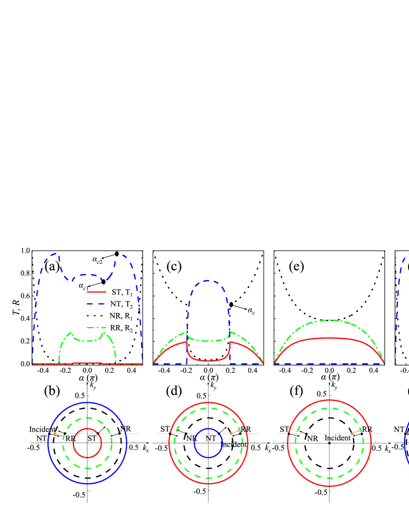
In Fig. 2(a), the reflection and transmission probabilities are plotted as a function of the incident angle at the interface of a step potential barrier. The electrons are incident with wave vector . The barrier height and incident energy are set as =0.5 and =0.1, respectively. The corresponding iso-energy lines for the incident and transmitted regions are presented in Fig. 2(b). The radii of these concentric circles from the innermost to the outermost are , , , and . Given that both the reflection and transmission probabilities are even functions concerning the incident angle , our discussions focus on the results for . When is small, as indicated by the horizontal dashed line in Fig. 2(b), double reflections and double transmissions can be generated because the four states are all propagating modes. Among the four propagating modes indicated in Fig. 2(b), the incident state lies between the NT state and the RR state, which indicates that the incident state is easier scattering into them as expressed in Eqs. (6)-(9). Hence, the probabilities of NT () and RR () are much larger than those of ST () and NR (). Owing to the presence of ST, fails to achieve its maximum value at normal incidence, which is different from the potential scattering in conventional semiconductors Griffiths . increases with the escalating , whereas, exhibits a gradual decreases as increases until it reaches the first critical angle ==0.14 where the horizontal dashed line becomes tangent to the red solid circle in Fig. 2(b). For , the ST state becomes evanescent wave, then vanishes. However, increases to a peak () as increases until it reaches the second critical angle ==0.26 where the horizontal dashed line becomes tangent to the green dashed circle in Fig. 2(b). Finally, rapidly diminishes to zero as approaches . Meanwhile, displays opposite trends compared to with an increasing up to , shown by the green dash- dotted line in Fig. 2(a). For , the RR state becomes evanescent wave, and vanishes, leading to a sharply increased .
Figures 2(c) and 2(e) display the reflection and the transmission as a function of the incident angle , in which electrons are incident with wave vector . The incident energies are =, and the barrier hight are and for Figs. 2(c) and 2(e), respectively. The corresponding iso-energy lines for the incident and transmitted regions are presented in Figs. 2(d) and 2(f). The radii of these concentric are also in the order of , , , and . For small barrier =, there are also four propagating states for small as indicated by the horizontal dashed line in Fig. 2(d). Consequently, double reflections and double transmissions also appear. Among the four propagating modes, the incident state lies between the NT state and the RR state, which means that the incident state is easier scattering into them as expressed in Eq. (13). Therefore, and are much larger than and . Different from the results in Fig. 2(a), reaches its maximum value at normal incidence and then decreases to zero when increases to the critical angle where the horizontal dashed line becomes tangent to the red solid circle in Fig. 2(d). For , vanishes because the NT state becomes evanescent wave. Whereas, increases with escalating and achieve its maximum at , then it gradually diminishes to zero as approaches . Meanwhile, displays opposite trends compared to , and shows the same trends compared to with the increasing of . For large barrier , such as =, the iso-energy circle corresponding to NT reduces to a point or disappears, and the ST state becomes evanescent wave. Hence, there are double reflections but only specular transmission in this case. Owing to the disappear of , is greatly enhanced compared with the results in Figs. 2(a) and 2(c). For electrons with incident energy satisfying , there are only two modes of propagation, one incident state and one reflected state. The scattering caused by the step barrier is similar to that in conventional semiconductors. Figure 2(g) plots the reflection and transmission spectra as a function of with and barrier hight . In this case, there are only SR () and NT (), as shown by the black solid and the blue dotted lines, respectively. The decreases slowly first and then drop fast with the increase of the , whereas, demonstrates a reversal behaviour, which is similar to the results in conventional semiconductors Griffiths . The reason is that only the NT and SR states are propagating modes within the whole incident angle range, as shown by the iso-energy lines in Fig. 2(g).
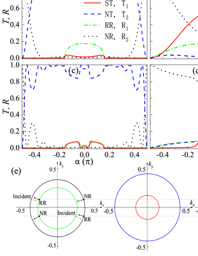
Next, let’s turn to the scattering induced by a rectangle potential barrier. Figures 3(a)-(d) show the reflection and the transmission spectra as a function of the incident angle for the scattering induced by a rectangle potential barrier for different barrier widths. In comparison to the results of the stepped barrier, there are two notable features in the case of the rectangle barrier. One is that the probability of ST will increase because there are two forward propagating waves in the barrier region [see Eq. (20)], and both of them produce ST at the interface . Another is that there is resonant tunnelling. We will focus on these two features in the following discussions.
For electrons incident with wavevector , as shown in Figs. 3(a) and 3(c), there is a critical angle = where the horizontal dashed line becomes tangent to the red solid circle in Fig. 3(e) in the reflection and transmission spectra. There are double reflections and transmissions for with enhanced and reduced because both the two forward propagating waves produce ST at the interface . However, and disappear for , and () shows some resonate peaks (dips), i.e., =1 (=0), as the increasing of arising from the resonate tunnelling. The resonate condition can be obtained numerically and need to be discussed in two cases because it sensitively depends on . For , the wavevectors and both are real. We have numerical checked the resonate condition and found it requires either =1 and =1 or =1 and =1. Therefore, we have = and =, where and are both odd or even. The resonate condition indicates large barrier width is needed to generate resonate tunnelling for . Hence, we only observe resonate tunneling within this angle region for =50 in Fig. 3(c). For , the wavevector becomes imaginary while is still real. By numerical calculation, we find the resonate condition becomes =1, i.e., = where is a nonzero integer, which is similar to that in conventional semiconductors Griffiths . The condition = means that the wider the potential barrier, the more the resonate peaks, which can be directly observed in Fig. 3(c) as indicated by the blue dashed line. For electrons incident with wavevector , as shown in Figs. 3(b) and 3(d), is greatly enhanced in comparison to the results induced by a stepped barrier. For a short barrier such as =10 nm, and doesn’t decrease to zero immediately when exceeds the critical angle [see Fig. 3(b)]. Although the states becomes evanescent wave, it can still penetrate a short barrier. For a wider barrier such as =50 nm, only shows some resonate peaks for . The resonate condition is also = and =, where and are both odd or even.
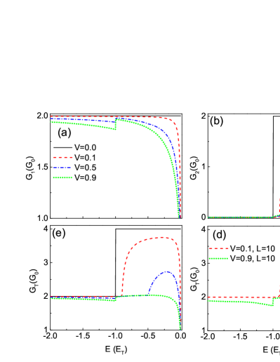
In order to understand the quantum transport properties of the junctions shown in Figs. 1(a) and 1(b). The ballistic conductances as a function of incident energy for the step and rectangle barriers are plotted in Fig. 4(a)-(d) with various potentials such as =0, 0.1, 0.5, and 0.9, where () denotes the conductance of electrons incident with (), and stands for the total conductance. As shown in Fig. 4(a), the conductance tends toward saturation with the decreasing incident energy for all barrier cases. The saturation conductance of diminishes as the barrier potential increases. This decrease in saturation conductance is attributed to the barrier obstructing the normal and specular transmissions, thereby causing an overall reduction in transmission. Concurrently, undergoes mutations at incident energy =. The magnitude of these mutations becomes more pronounced with larger values of , as the density of states in the transmitted region also undergoes mutation at . Conversely, as plotted in Fig. 4(b), initially experiences an ascent followed by a descent as the increasing of the incident energy for all barrier cases. takes its maximum around = ()/2, and gradually diminishes to zero at = (), giving rise to a negative differential conductance effect. This phenomenon can be elucidated by the fact that, when is below , the state in the transmission region becomes an evanescent wave, leading to a sharp decrease in the normal transmission as shown by the blue-dashed line in Fig. 3(e). Moreover, when is less than the brim of the Mexican-hat dispersion , the incident state becomes an evanescent wave, preventing transmission and resulting going straight to zero.
Now, let’s turn back to the total conductance depicted in Fig. 4(c) which is measured experimentally. As discussed in Figs. 4(a) and 4(b), tends to saturate with increasing incident energy, while sharply decreases. Consequently, the behavior of the total conductance =+ versus the incident energy is similar to that of . It also exhibits a negative differential conductance (NDC) effect. The transition energy of the NDC effect is . Initially, when the potential is absent, the peak-to-valley ratio of the NDC effect reaches a maximum value of 0.5 (see the black dashed line), but it gradually decreases with increasing . When the electrical potential exceeds , the NDC effect vanishes because there is only normal reflection and transmission in this case. Therefore, it is evident that the NDC effect can be effectively controlled by adjusting the barrier potential .
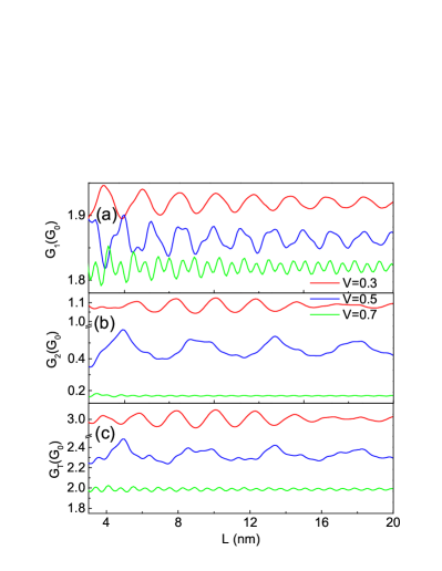
Figure 5 presents the conductances as a function of the barrier width for =0.4 under various potentials. As shown in Fig. 5, the conductances can be examined in two distinct scenarios. In the regime where , both and are real and there are four propagation modes within the barrier region, i.e., two forward and two backward. The oscillations of both and with respect to barrier width reveal a nuanced dynamic, characterized by the smaller oscillation period of compared to that of as indicated by the red and blue lines in Fig. 5(a) and 5(b). A discernible phase difference further distinguishes these oscillations. As the increasing of the barrier potential , the amplification of this period difference becomes evident, ushering in the emergence of multiple periods in the conductance . This phenomenon is particularly pronounced at elevated barrier potentials as shown in the red and blue lines in Fig. 5(c). As discussed in Fig. (4), the states matches the incident state better compared with the state . However, under the condition , the wavevector becomes imaginary while remains real. Consequently, persists in its oscillations with , while undergoes a substantial diminishment and cessation of oscillation as denoted by the green lines in Figs. 5(a) and 5(b). Consequently, in this distinctive scenario, the conductance is unequivocally dominated by the oscillatory behavior of as indicated by the green lines in Figs. 5(c).
IV Summary
In summary, we studied the quantum scattering and transport of electrons with Mexican-hat dispersion through both step and rectangular potential barriers by using the transfer matrix method. Owing to the torus-like iso-energy lines of the Mexican-hat dispersion, we observed the presence of double reflections and double transmissions in both two different barrier scenarios, i.e., the normal reflection (NR), retro-reflection (RR), normal transmission (NT), and specular transmission (ST). For the step potential with electrons incident from the large wavevector, the transmission is primarily governed by NT with nearly negligible ST, while the reflection is dominant by RR (NR) within (outside) the critical angle. Additionally, for electrons incident from the small wavevector, the NT can be reduced to zero by adjusting the barrier, resulting in a significant enhancement of ST and RR. For the rectangular barrier, the transmission and reflection spectra resemble those of the step barrier, but there are two kinds of resonant tunneling which can lead to perfect NT or ST. There exists a negative differential conductance (NDC) effect in the conductance spectrum. The conductance and the peak-to-valley ratio of the NDC effect can be effectively controlled by adjusting the height and width of the barrier as well as the incident energy. Our results provide a deeper understanding of the electron states governed by the Mexican-hat dispersion.
V Acknowledgments
This work was supported by the National Natural Science Foundation of China (Grant Nos. 12374071, 12174100, 12164021 and 11804092), and the Natural Science Foundation of Jiangxi Province (Grant No. 20212ACB201005).
References
- (1) K. S. Novoselov, A. K. Geim, S. V. Morozov, D. Jiang, Y. Zhang, S. V. Dubonos, I. V. Grigorieva, and A. A. Firsov, Science 306, 666 (2004).
- (2) H. Sahin, S. Cahangirov, M. Topsakal, E. Bekaroglu, E. Akturk, R. T. Senger, and S. Ciraci, Phys. Rev. B 80, 155453 (2009).
- (3) S. Yu, X. Wu, Y. Wang, X. Guo, and L. Tong, Adv. Mater. 29, 1606128 (2017).
- (4) M. Gibertini, M. Koperski, A. F. Morpurgo, and K. S. Novoselov, Nat. Nanotechnol. 14, 408 (2019).
- (5) G. Gao, G. Ding, J. Li, K. Yao, M. Wu, and M. Qian, Nanoscale 8, 8986 (2016).
- (6) H. Cai, Y. Gu, Y. C. Lin, Y. Yu, D. B. Geohegan, and K. Xiao, Appl. Phys. Rev. 6, 041312 (2019).
- (7) T. V. Vu, H. V. Phuc, L. C. Nhan, A. I. Kartamyshev, and N. N. Hieu, J. Phys. D: Appl. Phys. 56, 135302 (2023).
- (8) K. S. Novoselov, A. K. Geim, S. V. Morozov, D. Jiang, M. I. Katsnelson, I. V. Grigorieva, S. V. Dubonos, and A. A. Firsov, Nature 438, 197 (2005).
- (9) K. F. Mak, C. Lee, J. Hone, J. Shan, and T. F. Heinz, Phys. Rev. Lett. 105, 136805 (2010).
- (10) V. Zólyomi, N. D. Drummond, and V. I. Fal’ko, Phys. Rev. B 87, 195403 (2013).
- (11) S. J. Magorrian, V. Zólyomi, and V. I. Fal’ko, Phys. Rev. B 94, 245431 (2016).
- (12) H. R. Jappor and M. A. Habeeb, Current Applied Physics 18, 673 (2018).
- (13) M. Ariapour and S. T. Babaee, J. Magn. Magn. Mater. 510, 166922 (2020).
- (14) D. A. Bandurin, A. V. Tyurnina, G. L. Yu, A. Mishchenko, V. Zólyomi, S. V. Morozov, R. Krishna Kumar, R. V. Gorbachev, Z. R. Kudrynskyi, S. Pezzini, Z. D. Kovalyuk, U. Zeitler, K. S. Novoselov, A. Patanè, L. Eaves, I. V. Grigorieva, V. I. Fal’ko, A. K. Geim, and Y. Cao, Nat. Nanotechnol. 12, 223 (2017).
- (15) S. Demirci, N. Avazlı, E. Durgun, and S. Cahangirov, Phys. Rev. B 95, 115409(2017).
- (16) I. A. Kibirev, A. V. Matetskiy, A. V. Zotov, and A. A. Saranin, Appl. Phys. Lett. 112, 191602(2018).
- (17) Y. Jiang, S. Thapa, G. D. Sanders, C. J. Stanton, Q. Zhang, J. Kono, W. K. Lou, K. Chang, S. D. Hawkins, J. F. Klem, W. Pan, D. Smirnov, and Z. Jiang, Phys. Rev. B 95, 045116 (2017).
- (18) H. Min, B. Sahu, S. K. Banerjee, and A. H. MacDonald, Phys.Rev. B 75, 155115 (2007).
- (19) T. Hu, J. Zhou, and J. Dong, Phys. Chem. Chem. Phys. 19, 21722 (2017).
- (20) M. Zhou, R. Zhang, J. Sun, W. K. Lou, D. Zhang, W. Yang, and K. Chang, Phys. Rev. B 96, 155430 (2017).
- (21) B. Skinner, Phys. Rev. B 93, 235110 (2016).
- (22) X. B. Xiao, Q. Ye, Z. F. Liu, Q. P. Wu, Y. Li, and G. P. Ai, Nanoscale Res. Letts. 14, 322 (2019).
- (23) M. Nurhuda, A. R. T. Nugraha, M. Y. Hanna, E. Suprayoga, and E. H. Hasde, Adv. Nat. Sci: Nanosci. Nanotechnol. 11, 015012 (2020).
- (24) D. Wickramaratne, F. Zahid, and R. K. Lake, J. Appl. Phys. 118, 075101 (2015).
- (25) X. J. Ge, D. Qin, K. L. Yao, and J. T. Lü, J. Phys. D: Appl. Phys. 50, 405301 (2017).
- (26) L. Seixas, A. S. Rodin, A. Carvalho, and A. H. C. Neto, Phys. Rev. Lett. 116, 206803 (2016).
- (27) N. Ghobadi and A. Rezavand, Mater. Sci. Semicond. Process. 152, 107061 (2022).
- (28) T. Cao, Z. Li, and S. G. Louie, Phys. Rev. Lett. 114, 236602(2015).
- (29) M. Houssa, R. Meng, K. Iordanidou,G. Pourtoi, V. V. Afanasev, and A. Stesmans, J. Comput. Electron. 20, 88 (2021).
- (30) V. Zólyomi, N. D. Drummond, and V. I. Fal’ko, Phys. Rev. B 89, 205416 (2014).
- (31) J. P. Heremans, V. Jovovic, E. S. Toberer, A. Saramat, K. Kurosaki, A. Charoenphakdee, S. Yamanaka, and G. J. Snyder, Science 321, 554 (2008).
- (32) M. Zhou, D. Zhang, S. Yu, Z. Huang, Y. Chen, W. Yang, and K. Chang, Phys. Rev. B 99, 155402 (2019).
- (33) M. Zhou, S. Yu, W. Yang, W. K. Lou, F. Cheng, D. Zhang, and K. Chang, Phys. Rev. B 100, 245409 (2019).
- (34) D. J. Griffiths, Introduction to Quantum Mechanics (Cambridge University Press) (2016).
- (35) V. V. Cheianov, Vladimir Falko, and B L Altshuler, Science 315, 1252 (2007).
- (36) Gil-Ho Lee, Geon-Hyoung Park and Hu-Jong Lee, Nat. Phys. 11, 925 (2015).
- (37) Joanna Ruhl, Quantum Mechanics With a Quartic Dispersion, University of Massachusetts Boston, Doctoral Dissertations (2015).
- (38) M. Zhou, Phys. Rev. B 103, 155429 (2021).