[table]capposition=top
Parametric tuning of dynamical phase transitions in ultracold reactions
Abstract
Advances in ultracold chemistry have led to the possibility of a coherent transformation between ultracold atoms and molecules including between completely bosonic condensates. Such transformations are enabled by the magneto-association of atoms at a Feshbach resonance which results in a passage through a quantum critical point. In this study, we show that the presence of generic interaction between the formed molecules can fundamentally alter the nature of the critical point, change the yield of the reaction and the order of the consequent phase transition. We find that the correlations introduced by this rather general interaction induce nontrivial many-body physics such as coherent oscillations between atoms and molecules, and a selective formation of squeezed molecular quantum states and quantum cat states. We provide analytical and numerical descriptions of these many-body effects, along with scaling laws for the reaction yield in both the adiabatic and non-adiabatic regimes, and highlight the potential experimental relevance in quantum sensing.
I Introduction
Ultracold chemistry holds a prominent place in quantum engineering [1], information processing [2], and further understanding of fundamental quantum phenomena such as superconductivity, magnetism and mechanisms of elementary chemical reactions. One of the landmark experiments in the field of ultracold chemistry is the creation of Bose-Einstein condensates (BECs) using dilute gases of alkali metal atoms [3, 4, 5] in the 1990s. A series of experimental developments followed in the next two decades which led to major strides of progress in ultracold chemistry, quantum control and finally in the creation of a degenerate Fermi gas [6] and degenerate Bose gas of molecules [7], and observation of Bosonic stimulation of this reactive transformation [8].
Central to almost all the experimental developments concerning the creation of ultracold molecules is the concept of Feshbach resonance that allows for the association of bosonic/fermionic atoms by using a tunable magnetic field. Tuning a magnetic field across the Feshbach resonance drives an ultracold atomic system through a quantum critical point and hence a dynamical phase transition [9, 10] which results in the conversion of atoms to molecules. This ‘reaction’ is quantum coherent and reversible at macroscopic scale. The time-dependent Tavis-Cummings (TC) model [11] is a minimal model that captures many nontrivial many-body effects that are encountered during the stimulated reaction. Its Hamiltonian is
| (1) |
Here, () is the quantum mechanical pseudo-spin, and is the sweep rate of the transition through the Feshbach resonance. The sweep rate is controllable experimentally in a broad range – from almost instantaneous to quasi-adiabatic. The bosonic operator, , creates a molecule. The terms with the pseudo-spin raising and lowering operators, and , correspond, respectively, to the dissociation of a molecule and association of two fermionic atoms to form a bosonic molecule with a characteristic coupling (see [12, 13] for derivation of this model from true atomic-molecular Hamiltonians). The driven TC model can also be reformulated in terms of a fully bosonic reaction between bosonic atomic and molecular condensates [12, 13]. We will focus here on the reaction in which there are no molecules initially. This corresponds in (1) to the initial state, as , without molecules and the spin fully up-polarized along the -axis.
The time-dependent sweep is needed in practice to make all atoms encounter the resonance. In addition, the quantum adiabatic theorem guarantees that a sufficiently slow sweep converts the initial atomic state into the bosonic ground state, which is the molecular condensate. Hence, potentially, a 100% efficiency of the reaction is experimentally possible. However, the true adiabatic limit cannot be reached, so it is important to understand the quasiadiabatic regime with small but finite . This regime is characterized by the number of nonadiabatic excitations, , which is the number of the molecules that would appear in the adiabatic limit but did not form after the transition through the resonance, i.e., as .
An unusual theoretical finding about the time-dependent TC model was the discovery of its integrability [14, 15], which proved the existence of a dynamical phase transition and confirmed semiclassical predictions for the power-law scaling of the nonadiabatic excitation density after the quasi-adiabatic sweep through the resonance [12]. However, recent experiments [8] with a bosonic reaction show a behavior that is not known within the slowly driven TC model, such as coherent oscillations between atoms and molecules after crossing the Feshbach resonance. Moreover, even with the slowest sweep rates, a system usually ends up in a pre-thermalized atomic-molecular mixture state, in disagreement with the nearly perfect reaction efficiency predicted by the TC model [16].
One possibility to extend the TC model to account for the richer reaction dynamics is to add a dispersion of the atomic states. This results in a generalized TC model [15, 13] that, surprisingly, is also solvable but leads to essentially the same predictions for the behavior of the nonadiabatic excitations on the sweep rate as the minimal model (1). Hence, other interaction types may be responsible for the experimentally observed behavior beyond the standard TC model.
In this article, we consider a different generalization of the model (1), in which we add another molecular coupling term:
| (2) | |||
| (3) |
and where is the molecular number operator; is the coupling strength. The coupling in (3) is effectively broadening the molecular dispersion energy, which becomes now dependent on the number of molecules that changes during the reaction. Such a coupling must be present in ultracold molecules due to dipole interactions and elastic scatterings.
We find that this addition to the model leads to a substantially richer behavior, especially for quasi-adiabatic transitions. This could be anticipated from the applications of the TC model in optics, where such a nonlinear term describes the optical mode in a ‘Kerr-like’ medium [17, 18, 19].
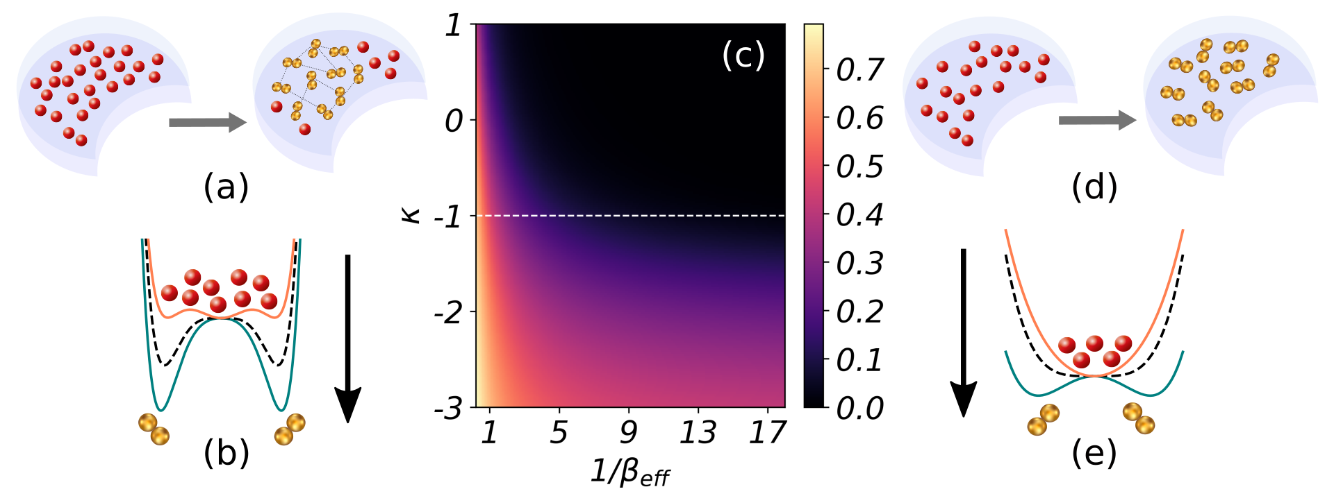
With this addition, the phase diagram for the reaction efficiency depends on both the sweep rate and the nonlinearity . In Fig. 1 we show the result of our numerical simulations for the number of the nonadiabatic excitations, which is the number of unformed molecules, following the sweep of the chemical potential. By setting , the line marks a critical nonlinearity, such that for the number of the nonadiabatic excitations is much larger than for , especially in the quasi-adiabatic limit (large ). We will show that this behavior follows from the possibility of either a second- or first-order phase transition during the sweep through the Feshbach resonance. Our model is no longer exactly solvable but in the quasi-adiabatic limit it can be studied analytically in detail.
II Semiclassical description and phase transitions
The experimentally relevant regime corresponds to a large number of molecules, , that can be potentially created during the sweep through the resonance. This justifies the semiclassical approximation. To develop it, first, we note that our model conserves
| (4) |
whose eigenvalue corresponds to our initial conditions, where the starting state is the one without molecules. Hence, it is convenient to mark all states by the number of molecules:
where is the state with molecules and is the spin state with . The initial state as corresponds to . The matrix elements in this basis are given by
| (5) |
Let us look for the solution to the Schrödinger equation of the form , and introduce the amplitude generating function
| (6) |
Note that , so the time-dependent Schrödinger equation for the amplitudes can be written in terms of a single equation for as
| (7) |
where we associate . In the semiclassical approximation we can then associate with a coordinate that is conjugate to the classical momentum . In addition, we disregard the terms of order . Then, the classical Hamiltonian that corresponds to the Schrödinger equation (7) has the form
| (8) |
with a time-dependent parameter
and the classical equations of motion
| (9) |
III Quasi-adiabatic second-order phase transition
Up to the new -dependent nonlinear term, the Hamiltonian (8) coincides with the analogous semiclassical Hamiltonian in [12]. The relation between the classical variables and the number of the nonadiabatic excitations is established by noting that as the time-dependent term completely dominates: . Following [12], we note that the equations of motion initially conserve and the adiabatic invariant is given by the initial number of molecules, :
If during the evolution the adiabatic invariant acquires a small contribution , this is interpreted in the semiclassical theory as the density of the produced elementary nonadiabatic excitations, i.e, . In the strict adiabatic limit, the ground state with no molecules eventually is transferred into the new ground state with molecules. Taking into account the nonadiabatic excitations, the number of the created molecules in our process is given by
We should assume that initially , which is negligible in comparison to the large . Next, we assume a nearly adiabatic sweep of the chemical potential [12]. The point is a steady point of the classical equations (9), in the vicinity of which the system evolves. Assuming that near this point , and retaining the terms of the lowest order we find an effective Hamiltonian that governs the evolution at the early stage of the reaction, that is
| (10) |
For a quasi-adiabatic evolution, the nonadiabatic excitations are generally suppressed exponentially, as , with some finite positive . Such excitations are not essential and we can safely disregard them. However, according to the Kibble-Zurek phenomenology, the excitations are enhanced near a critical point, at which the symmetry of the original ground state breaks down spontaneously. It turns out that the Hamiltonian (10) contains this event, so it is sufficient to describe the phase transition quantitatively.
We shift the zero of time by setting:
| (11) |
and make a canonical transformation in (10):
| (12) |
leading to an effective classical time-dependent Hamiltonian for a single degree of freedom:
| (13) |
where now is treated as the momentum and as the coordinate.
Suppose that . This corresponds to either repulsive () or weakly attractive () interactions between the formed molecules. If were a constant, then the Hamiltonian (13) would describe a nonlinear oscillator with the potential energy
| (14) |
The initial conditions correspond to . In fact, a quantum mechanical treatment of the initial conditions needs averaging of the behavior over a distribution of small initial values with [12]. However, we will show later that this information is irrelevant within the leading order semiclassical description. The system with the potential (14) experiences the 2nd order phase transition at . Indeed, for , the potential has a single minimum at but for , there are two local minima at .
In Fig. 1, we illustrate that for the system is initially near a single minimum but it follows one of the new minima for . In phase space, this corresponds to crossing a separatrix, in which vicinity the classical adiabatic invariant is no longer conserved. Thus, so far our approximations were justified because they capture the main source of the nonadiabatic excitations near the phase transition.
The evolution equations for and with the Hamiltonian (10), acquire a universal form after re-scaling of the variables:
and
where , , and are constants. We choose them so that in terms of the rescaled variables has the form with only numerical coefficients
| (15) |
In the new variables, the equations of motion have the canonical form of the Painlevé-II equation
| (16) |
The dynamics does not depend anymore on the relative values of the parameters and . However, we reiterate that at , the model is exactly solvable, so all known facts about the solution of the driven TC model can now be applied to the dynamics according to Eq. (16).
The rescaling of variables, however, was not canonical, so it did not conserve the action:
Hence, if is the adiabatic invariant in the original variables, and , then in the rescaled and the invariant is given by . For our case, we found
| (17) |
Equation (17) can be used to establish the relation between the exactly solvable case at and our more general model for . Namely, for , the scaling for the number of the excitations was found to be a power law with a logarithmic prefactor [15] (for earlier but only semiclassical derivations of this formula at , see also discussion around Eq. (11) in [20] and Eq. (15) in [21]):
| (18) |
where either the exact solution or further semiclassical analysis can be used to fix for our initial conditions in the model (1). According to [15], this result is valid only in the quasi-adiabatic case, namely for . For example, at , in this range Eq. (18) coincides with the exactly found expression for the position of the maximum of the probability distribution of the excitation number.
Using (17), and the fact that all values lead to the universal Eq. (16), we can now extend the result in (18) to the case with arbitrary by properly rescaling the action variables:
| (19) |
where is the parameter of order that characterizes the initial conditions. As this unknown factor appears inside the logarithm in (19), its precise value is not important because its relative contribution to (19) vanishes in the limit for the quasi-adiabatic evolution with . For comparison with numerical results, we set .
Thus, Eq. (19) extends the expression known in the exactly solvable case, for , by merely re-scaling the coupling as
| (20) |
for a general value of . In terms of the parameter , this corresponds to the re-scaling . The smaller sweep rates, , are not captured by the formula (19) because this regime corresponds to the onset of the truly adiabatic evolution, with exponentially suppressed excitations. For experimentally relevant values, , this truly adiabatic regime cannot be reached, so we leave it without further discussions.
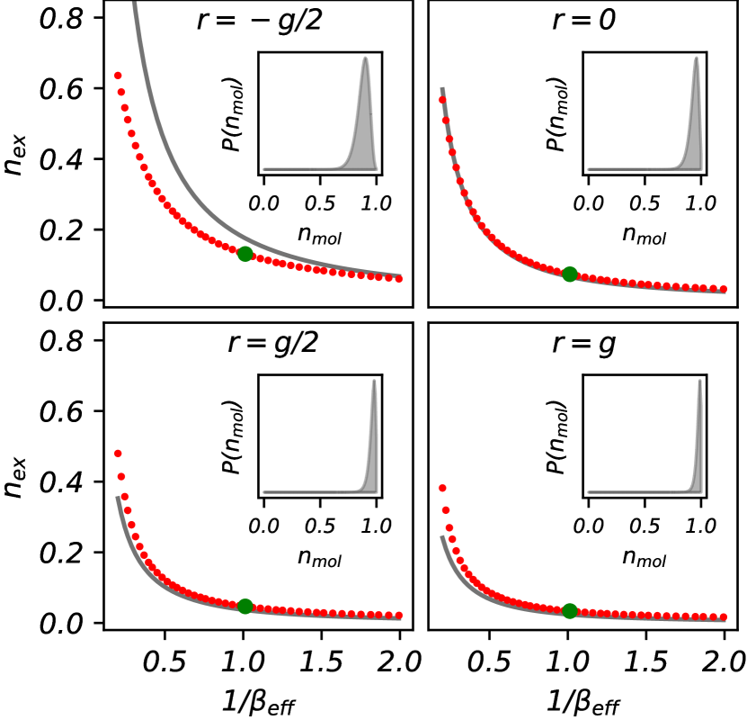
The change of the adiabatic invariant is interpreted in terms of the density of the nonadiabatic excitations: , which in turn is related to the deviation of the average number of the formed molecules from its maximal value. Our analysis so far has been restricted to the quasi-adiabatic regime. A comparison with numerical results is shown in Fig. 2. The agreement for the interval is indeed found. However, beyond this interval the deviations from our formulas are strong. Note also that these deviations persist to smaller when approaches the value , indicating the breakdown of our analysis for .
In summary, our theory predicts the robustness of the 2nd order dynamical phase transition for repulsive and moderate attractive interactions (). Its signature in experiments can be the scaling of the density of the excitations (unformed molecules) for different sweep rates in the quasi-adiabatic regime:
which is the same as in the exactly solvable case at .
IV First-order phase transition
The energy (10) has no finite global minimum for , so we must include the next order term, in the effective Hamiltonian (10). After the transformations (11) and (12), we find
| (21) |
Disregarding the higher order terms in and is justified when the main nonadiabatic effects occur for . This requires that
In addition, we should assume the same initial conditions as in the previous case, . Consider now only the potential energy
As , it has a single energy minimum at . With time, two additional energy minima initially appear at higher energy but eventually become the global minima of . However, the transition into them, for some time, is classically forbidden due to the energy barriers.
By approaching the time moment the minimum at becomes initially a false vacuum, and for it becomes an unstable local maximum. The steady point at can then be perturbed by any quantum fluctuation, so at the system has to fall towards one of the remaining minima, which at this moment are given by
with corresponding energy . The system can choose to be in one of the two minima with equal probability. At this point, let us consider that the system escapes towards .
At , the energy of the false vacuum state is . Hence, along the escape trajectory the momentum is given by
| (22) |
The turning points of this trajectory are at and and its adiabatic invariant is
| (23) |
Since the initial value of the adiabatic invariant is , to leading order in , the density of excitations is associated with the invariant (23):
| (24) |
which is independent of the sweep rate , as long as we consider the quasi-adiabatic dynamics and disregard the exponentially suppressed quantum tunneling events. Thus, the first-order phase transition is associated with a finite density of the excitations even in the quasi-adiabatic regime. We note also that an almost perfect efficiency of ultracold chemical reactions has so far not been achieved experimentally even for the slowest sweeps through the Feshbach resonance. This may be an indication of the presence and importance of molecular interactions of the type that we have considered here.
Equation (24) explains the sharp transition in observed around in Fig. 1, in the quasi-adiabatic regime. Qualitatively similar saturation of the number of excitations was found previously in the nonlinear Landau-Zener model [22], in which this behavior was not related to a spontaneous symmetry breaking. The dependence of on for different values of with (or ) are plotted in Fig. 3, confirming the saturation of at a finite value in the adiabatic limit.
The -dependent correction to Eq. (24) deserves a discussion. For small , this correction can be considerable because the saturation value of in (24) scales on as , whereas for the -dependent component we provide the scaling arguments (Methods) showing that at the excitations are suppressed with decreasing too slowly to be completely eliminated in our numerical simulations. At fixed , this -dependent contribution changes linearly with a small :
| (25) |
We plot the dependence of on in the nonadiabatic regime in Fig. 3. Our numerical Fig. 3 was obtained by looking at the changes of at smallest possible but finite . Hence, only the slope of the line but not the constant offset from the axes origin could be compared to Eq. (24).
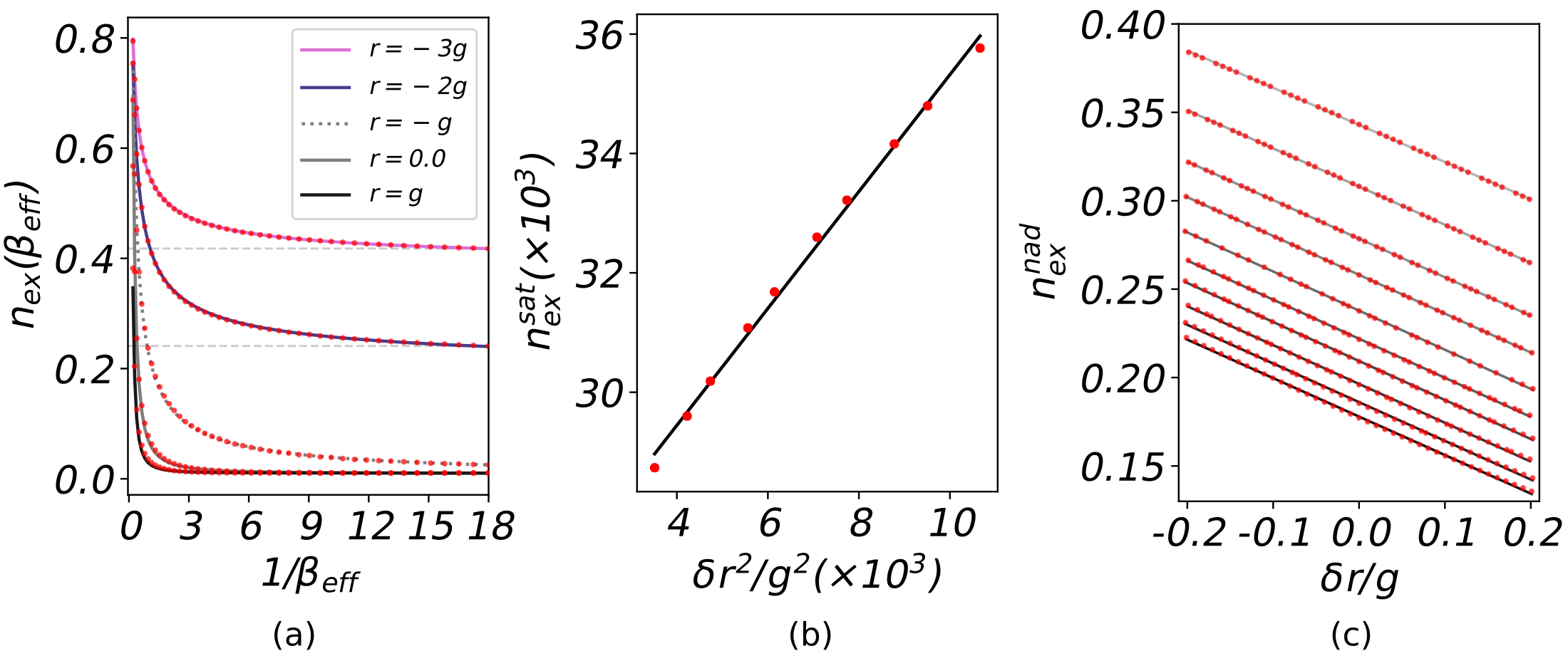
In general, for a finite sweeping rate , we also have a Kibble-Zurek scaling of the number of excitations:
| (26) |
where the exponent depends on . In the Methods section, we estimated this exponent analytically for () to be , which is different from the exponent of the second-order phase transition (see Fig. 3 for numerical proof). For , we have numerically, together with (24):
| (27) |
where is independent of .
Previously, a similar scaling was observed for the formation of topological defects in the dynamics of a classical field undergoing a weakly first-order phase transition at finite temperature [23]. Here, we have obtained a similar result for a fully coherent evolution through a quantum phase transition at zero temperature.
V Transient dynamics and prethermalization
A characteristic dynamical feature accompanying the phase transition at time is the oscillation of atomic and molecular populations which become rapidly damped with time. Such transient oscillations of the number of molecules are usually observed in the nonadiabatic regime but become suppressed in the adiabatic limit for a typical second-order phase transition. However, we found that the transient state in the case of a first-order phase transition remains persistent and highly nonclassical.
This is manifested as a complex series of collapse and revival of the number of molecules as a function of time (see Fig. 4). This pattern is particularly prominent in the adiabatic limit. We note that such patterns have been encountered previously in the time-independent versions of the Jaynes-Cummings model [24], Bose-Hubbard model [25], a model of nonlinear directional couplers [26], and even in a generalized version of the model in (1) but at other conditions [27].
In our model, in the case of the second-order transition, these collapse-revival oscillations are absent (see Fig. 4). The quasi-adiabatic regime then produces a sharply-peaked molecular number distribution. In contrast, the number distribution for the first-order transition is very broad, which indicates a phase squeezing. As discussed for related models in [25, 28], such collapse-revival patterns are a purely quantum-mechanical phenomenon; the semiclassical Hamiltonian in (8) does not predict these features.
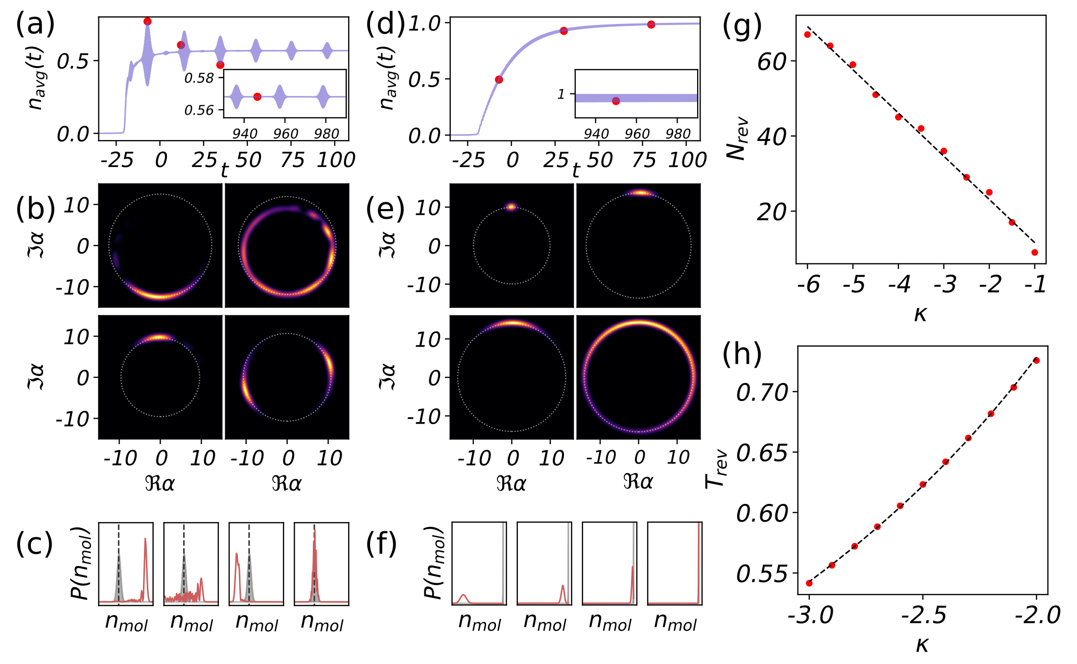
To further understand the characteristics of this collapse-revival oscillations, we generated projections of the time-dependent molecular wavefunction onto the basis of coherent states, as shown in Fig. 4. It reveals that the collapse and revival patterns constitute an oscillation of the number distribution about the asymptotic limit (marked in gray in Fig. 4). We also found that the number of revivals per unit time increases linearly with the strength of nonlinearity () for the first-order transition. The frequency of the collapse-revival patterns decreases gradually following the sweep, and in general saturates to a constant value resulting in a punctuated series of revivals that survive for a very long time. The time-period of any particular collapse and revival pair also decreases with as
| (28) |
We plot the numerically found dependence of and on in Fig. 4. The sustained oscillation pattern and the dependence of the frequency and time period on the interaction strength are reminiscent of the prethermalized states [29] that were numerically observed [30, 31] following a sudden quench in bosonic/fermionic Hubbard models. A main aspect of such nonequilibrium states is the existence of long-time memory of the initial conditions as in our model.
One of the main consequences of this long-term memory and inherently nonequilibrium dynamics of the prethermalized state is the generation of a quantum cat state in the limit of the forward sweep (see Fig. 4 showing the snapshots for time-evolution in the Glauber basis). In the limit , after the adiabatic first-order transition, the dynamics eventually freezes in a superposition of two macroscopically distinguishable states (shown as the bottom-right panel in Fig. 4). Each of these states in the Glauber basis is localized, and therefore is similar to a macroscopic Bose-Einstein condensate with a well defined phase. However, the phases of the condensates in the cat state are different by . Thus, even the prethermalized state of the nonadiabatic excitations is strongly nonclassical.
VI Discussion
We have explored the role of molecular interactions in mediating dynamic phase transitions in ultracold chemistry with an extension of the Tavis-Cummings model. The standard integrable driven Tavis-Cummings model has made several predictions which should be observable in experiments that associate ultra-cold atoms into molecules by a stimulated passage through the Feshbach resonance. We tested the robustness of these predictions against additional molecular interactions that break the model’s integrability. For moderate interactions we found that, as in the integrable case, the system passes through the second-order phase transition. In the quasi-adiabatic regime, this leads to a nearly linear scaling, , of the number of the unformed molecules on the sweep rate .
Above a certain critical interaction strength, the order of the phase transition changes from the second to the first, with drastic changes in the reaction dynamics. The main characteristic of the crossover to the first-order phase transition is that even in the adiabatic limit the density of the excitations remains finite. Accompanying this is a transient dynamics that manifests as pronounced oscillations in the molecular population. Asymptotically, the system reaches a prethermalized state (Fig. 4), which is a strongly nonclassical superposition of two condensate-like states with a phase difference of between them, a feature which is absent in the typical case of the second-order phase transition.
Such dynamical features, which are usually attributed to the strongly nonadiabatic regime (e.g., following a sudden quench, as in [30, 31, 32, 29, 33]), are observed in our model (2), during the quasi-adiabatic transition through a first-order critical point. This has a potential impact on the endeavours in creating non-classical states such as the macroscopic cat states and squeezed states in bosonic systems, which are of utmost importance in quantum sensing and metrology [34]. In the past, several experiments have targeted the creation of such non-classical states [35, 36, 37], some of which used a Kerr-type nonlinearity to stabilize these states. Given that the size of an atomic cloud is of the order of , the passage through the Feshbach resonance with a first-order phase transition presents an attractive opportunity to create practically desired strongly nonclassical macroscopic states.
Apart from applications in quantum sensing, experiments in ultracold chemistry also serve to demonstrate the universality of the dynamics around quantum phase transitions [38]. For instance, there is considerable evidence (both theoretical and observational) that phase transitions occurred during the early evolution of our universe [39]. Our study reveals that purely quantum correlations play a considerable role in such processes, and that the nature of the quantum critical point is manifested in the scaling of the excitation density. The main experimental challenge in studying such correlations will be in tuning the interaction strength and obtaining the desired degree of quantum control. With major strides of experimental development in ultracold chemistry in the last decade, we expect this to be possible in the near future.
VII Methods
VII.1 Numerical simulations
The time-dependent Schrödinger equation that describes the time evolution of the Hamiltonian (2) was propagated using the Trotter-factorized discretization of the unitary propagator. Since (2) is also sparse (as is evident from (5)), the time complexity of the cost of the propagation scales almost linearly with .
VII.2 Husimi-Q projection
The coherent Husimi Q projection of the wavefunction in the molecule number basis (Fig. 4) was obtained as:
| (29) | ||||
| (30) |
where corresponds to the projection onto a coherent state indexed by and is the amplitude of the wavefunction in the molecular population basis .
VII.3 Scaling exponent beyond Painleve-II equation
When a Hamiltonian has a time-dependent perturbation , the nonadiabatic tunneling probability is computed from the change in the curvature (or frequency) [40] as:
| (31) |
Following the approach in [22], to evaluate the scaling behaviour of , we express in terms of . In the case of the first-order transition, the major change in the curvature occurs at the point (see (11)) after which increases in time. We consider the dynamical equations given by the Hamiltonian (8) in terms of the scaled time variable which yields:
| (32) | ||||
| (33) |
where and . It is straightforward to see that the rate of change of is given as:
| (34) |
The reason for the inclusion of a logarithmic term in the above expression is explained in [13]: for a given , the is the point of discontinuity in the behaviour of vs (see Eq. (13) in [13] and note that the parameter in [13] differs from the in this article by a factor of ).
Around the fixed point , for , this yields:
| (35) |
from which we get:
| (36) |
This gives the following expressions:
| (37) | ||||
| (38) |
which we confirmed numerically in Fig. 3. In general, we found that such a power-law scaling holds for all values of , but an analytical derivation of the corresponding exponent was not possible.
For the near-critical case with , we get:
| (39) |
Expanding upto linear order in , we get:
| (40) |
where
| (41) |
(we numerically found a weak dependence of with respect to ). Note that the sign of is positive: when increases, the tunneling probability goes up (which can be inferred from fig. 1. For a constant , we hence have:
| (42) |
Thus, the concentration of defective excitations increases linearly with , which is also evident from Figs. 1 and 3.
VIII Acknowledgement
This work was supported in part by the U.S. Department of Energy, Office of Science, Office of Advanced Scientific Computing Research, through the Quantum Internet to Accelerate Scientific Discovery Program, and in part by U.S. Department of Energy under the LDRD program at Los Alamos. V.G.S. acknowledges funding from St. John’s College, Cambridge for travel, and the Yusuf Hamied Department of Chemistry, Cambridge for computing resources. F.S. acknowledges support from the Center for Nonlinear Studies. We also thank Yair Litman and Paramvir Ahlawat for their scientific comments which improved the presentation style of the manuscript.
References
- Bohn et al. [2017] J. L. Bohn, A. M. Rey, and J. Ye, Cold molecules: Progress in quantum engineering of chemistry and quantum matter, Science 357, 1002 (2017).
- Baranov et al. [2012] M. A. Baranov, M. Dalmonte, G. Pupillo, and P. Zoller, Condensed matter theory of dipolar quantum gases, Chem. Rev. 112, 5012 (2012).
- Anderson et al. [1995] M. H. Anderson, J. R. Ensher, M. R. Matthews, C. E. Wieman, and E. A. Cornell, Observation of Bose-Einstein condensation in a dilute atomic vapor, Science 269, 198 (1995).
- Davis et al. [1995] K. B. Davis, M. O. Mewes, M. R. Andrews, N. J. van Druten, D. S. Durfee, D. M. Kurn, and W. Ketterle, Bose-Einstein condensation in a gas of sodium atoms, Phys. Rev. Lett. 75, 3969 (1995).
- Bradley et al. [1995] C. C. Bradley, C. A. Sackett, J. J. Tollett, and R. G. Hulet, Evidence of Bose-Einstein condensation in an atomic gas with attractive interactions, Phys. Rev. Lett. 75, 1687 (1995).
- De Marco et al. [2019] L. De Marco, G. Valtolina, K. Matsuda, W. G. Tobias, J. P. Covey, and J. Ye, A degenerate Fermi gas of polar molecules, Science 363, 853 (2019).
- Zhang et al. [2021] Z. Zhang, L. Chen, K.-X. Yao, and C. Chin, Transition from an atomic to a molecular Bose–Einstein condensate, Nature 592, 708 (2021).
- Zhang et al. [2023] Z. Zhang, S. Nagata, K.-X. Yao, and C. Chin, Many-body chemical reactions in a quantum degenerate gas, Nat. Phys. , 1 (2023).
- Romans et al. [2004] M. Romans, R. Duine, S. Sachdev, and H. Stoof, Quantum phase transition in an atomic Bose gas with a Feshbach resonance, Phys. Rev. Lett. 93, 020405 (2004).
- Radzihovsky et al. [2004] L. Radzihovsky, J. Park, and P. B. Weichman, Superfluid transitions in bosonic atom-molecule mixtures near a Feshbach resonance, Phys. Rev. Lett. 92, 160402 (2004).
- Yurovsky et al. [2002] V. Yurovsky, A. Ben-Reuven, and P. S. Julienne, Quantum effects on curve crossing in a Bose-Einstein condensate, Phys. Rev. A 65, 043607 (2002).
- Altland et al. [2009] A. Altland, V. Gurarie, T. Kriecherbauer, and A. Polkovnikov, Nonadiabaticity and large fluctuations in a many-particle Landau-Zener problem, Phys. Rev. A 79, 042703 (2009).
- Malla et al. [2022] R. K. Malla, V. Y. Chernyak, C. Sun, and N. A. Sinitsyn, Coherent reaction between molecular and atomic Bose-Einstein condensates: integrable model, Phys. Rev. Lett. 129, 033201 (2022).
- Sinitsyn and Li [2016] N. A. Sinitsyn and F. Li, Solvable multistate model of Landau-Zener transitions in cavity QED, Phys. Rev. A 93, 063859 (2016).
- Sun and Sinitsyn [2016] C. Sun and N. A. Sinitsyn, Landau-Zener extension of the Tavis-Cummings model: Structure of the solution, Phys. Rev. A 94, 033808 (2016).
- Chin et al. [2010] C. Chin, R. Grimm, P. Julienne, and E. Tiesinga, Feshbach resonances in ultracold gases, Rev. Mod. Phys. 82, 1225 (2010).
- Bužek and Jex [1990] V. Bužek and I. Jex, Dynamics of a two-level atom in a Kerr-like medium, Opt. Commun. 78, 425 (1990).
- Agarwal and Puri [1989] G. Agarwal and R. Puri, Collapse and revival phenomenon in the evolution of a resonant field in a Kerr-like medium, Phys. Rev. A 39, 2969 (1989).
- Gora and Jedrzejek [1992] P. Gora and C. Jedrzejek, Nonlinear Jaynes-Cummings model, Phys. Rev. A 45, 6816 (1992).
- Gurarie [2009] V. Gurarie, Feshbach molecule production in fermionic atomic gases, Phys. Rev. A 80, 023626 (2009).
- Itin and Törmä [2010] A. P. Itin and P. Törmä, Dynamics of quantum phase transitions in Dicke and Lipkin-Meshkov-Glick models, Preprint arXiv:0901.4778 (2010).
- Liu et al. [2002] J. Liu, L. Fu, B.-Y. Ou, S.-G. Chen, D.-I. Choi, B. Wu, and Q. Niu, Theory of nonlinear Landau-Zener tunneling, Phys. Rev. A 66, 023404 (2002).
- Suzuki and Zurek [2023] F. Suzuki and W. H. Zurek, Topological defect formation in a phase transition with tunable order, Preprint arXiv:2312.01259 (2023).
- Shore and Knight [1993] B. W. Shore and P. L. Knight, The Jaynes-Cummings model, J. Mod. Opt. 40, 1195 (1993).
- Milburn et al. [1997] G. Milburn, J. Corney, E. M. Wright, and D. Walls, Quantum dynamics of an atomic Bose-Einstein condensate in a double-well potential, Phys. Rev. A 55, 4318 (1997).
- Chefles and Barnett [1996] A. Chefles and S. M. Barnett, Quantum theory of two-mode nonlinear directional couplers, J. Mod. Opt. 43, 709 (1996).
- Santos et al. [2006] G. Santos, A. Tonel, A. Foerster, and J. Links, Classical and quantum dynamics of a model for atomic-molecular Bose-Einstein condensates, Phys. Rev. A 73, 023609 (2006).
- Greiner et al. [2002] M. Greiner, O. Mandel, T. W. Hänsch, and I. Bloch, Collapse and revival of the matter wave field of a Bose–Einstein condensate, Nature 419, 51 (2002).
- Ueda [2020] M. Ueda, Quantum equilibration, thermalization and prethermalization in ultracold atoms, Nat. Rev. Phys. 2, 669 (2020).
- Kollath et al. [2007] C. Kollath, A. M. Läuchli, and E. Altman, Quench dynamics and nonequilibrium phase diagram of the Bose-Hubbard model, Phys. Rev. Lett. 98, 180601 (2007).
- Eckstein et al. [2009] M. Eckstein, M. Kollar, and P. Werner, Thermalization after an interaction quench in the Hubbard model, Phys. Rev. Lett. 103, 056403 (2009).
- Birnkammer et al. [2022] S. Birnkammer, A. Bastianello, and M. Knap, Prethermalization in one-dimensional quantum many-body systems with confinement, Nat. Commun. 13, 7663 (2022).
- Kaminishi et al. [2015] E. Kaminishi, T. Mori, T. N. Ikeda, and M. Ueda, Entanglement pre-thermalization in a one-dimensional bose gas, Nat. Phys. 11, 1050 (2015).
- Pirandola et al. [2018] S. Pirandola, B. R. Bardhan, T. Gehring, C. Weedbrook, and S. Lloyd, Advances in photonic quantum sensing, Nat. Photon. 12, 724 (2018).
- Kirchmair et al. [2013] G. Kirchmair, B. Vlastakis, Z. Leghtas, S. E. Nigg, H. Paik, E. Ginossar, M. Mirrahimi, L. Frunzio, S. M. Girvin, and R. J. Schoelkopf, Observation of quantum state collapse and revival due to the single-photon Kerr effect, Nature 495, 205 (2013).
- Ourjoumtsev et al. [2011] A. Ourjoumtsev, A. Kubanek, M. Koch, C. Sames, P. W. Pinkse, G. Rempe, and K. Murr, Observation of squeezed light from one atom excited with two photons, Nature 474, 623 (2011).
- Grimm et al. [2020] A. Grimm, N. E. Frattini, S. Puri, S. O. Mundhada, S. Touzard, M. Mirrahimi, S. M. Girvin, S. Shankar, and M. H. Devoret, Stabilization and operation of a Kerr-cat qubit, Nature 584, 205 (2020).
- Clark et al. [2016] L. W. Clark, L. Feng, and C. Chin, Universal space-time scaling symmetry in the dynamics of bosons across a quantum phase transition, Science 354, 606 (2016).
- Mazumdar and White [2019] A. Mazumdar and G. White, Review of cosmic phase transitions: their significance and experimental signatures, Rep. Prog. Phys. 82, 076901 (2019).
- Landau and Lifshitz [1982] L. Landau and E. Lifshitz, Mechanics: Volume 1, Elsevier Science, London (1982).