Experimental study of dynamic wetting behavior through curved microchannels with automated image analysis

Abstract

Preventing fluid penetration poses a challenging reliability concern in the context of power electronics, which is usually caused by unforeseen microfractures along the sealing joints. A better and more reliable product design heavily depends on the understanding of the dynamic wetting processes happening inside these complex microfractures, i.e. microchannels. A novel automated image processing procedure is proposed in this work for analyzing the moving interface and the dynamic contact angle in microchannels. In particular, the developed method is advantageous for experiments involving non-transparent samples, where extracting the fluid interface geometry poses a significant challenge. The developed method is validated with theoretical values and manual measurements and exhibits high accuracy. The implementation is made publicly available. The developed method is validated and applied to experimental investigations of forced wetting with two working fluids (water and 50 wt% Glycerin/water mixture) in four distinct microchannels characterized by different dimensions and curvature. The comparison between the experimental results and molecular kinetic theory (MKT) reveals that the dynamic wetting behavior can be described well by MKT, even in highly curved microchannels. The dynamic wetting behavior shows a strong dependency on the channel geometry and curvature.

1 Introduction

In recent years, with the automotive industry’s strategy moving towards vehicle electrification, power electronics with higher energy density and efficiency have received considerable attention along with stringent reliability constrains. Reliability of power electronics involves multiple aspects, including mechanical strength, corrosion resistance and media tightness etc. ([33]; [16]). A highly challenging task is to prevent the fluid penetration caused by the unforeseen microfracture along sealings and faulty joints as reported by [22]. These microfractures exhibit complex characteristics which hinder an instinctive prediction of possible penetration rates, hence, making a deeper understanding of the dynamic wetting behavior, characterized by the dynamic contact angle, is necessary for reliable product design.

Accurate, robust and automatic measurement of dynamic contact angles is crucial for experimental and numerical investigations of wetting processes. In this work, a novel automated image analysis procedure is proposed for the interface detection and dynamic contact angle measurement of capillary flows. The automated image analysis is first validated in 5.1, by comparing automatic measurements with theoretical values and manual measurements. The proposed automated procedure considerably speeds up experimental data analysis. An implementation of our procedure used in this manuscript is made publicly available at the TUDatalib data repository at TUDarmstadt ([37]), and at Bosch Research GitHub ([25]).

A robust, accurate, and automatic dynamic contact angle measurement provides a data for understanding dynamic wetting processes in capillaries. Dynamic wetting is very actively researched topic in interfacial science, combining analytical, experimental and numerical investigations ([36]), and generating a broad selection of models. Over the past decades, several theoretical approaches have been proposed to describe the dynamic wetting process, which comprise of hydrodynamic theory (HDT) for viscous dissipation during displacement of the contact line proposed by [31] and [17], molecular-kinetic theory (MKT) for the contact line friction dissipation in the vicinity of the contact line ([2]; [3]; [1]), the interface formation model (IFM) proposed by [28] and some combined models incorporating both HDT and MKT as published by [24] and [5].

For investigating the two mechanism for contact line dynamics, spontaneous and forced wetting, the main experimental setups found in literature for spontaneous wetting include droplet spreading ([15]; [13]; [6]; [35]) and capillary rise ([29]; [32]; [8]), while Wilhelmy plate ([21]; [23]; [20]) is a classical example for forced wetting. However, forced wetting through microchannels, which holds considerable more relevance in the context of industrial applications, shall be the focus of this paper’s investigation.

This work studies experimentally the dynamic wetting with small capillary number $Ca$ $(10^{-6}-10^{-3})$ in microchannels with different geometries (section 3), with the intention of covering common industrial circumstances in the context of media tightness and leakage. Two working fluids, water and 50 wt% Glycerin/water mixture are employed. The experimental results are compared with MKT model by applying curve-fitting method. The dynamic contact angle model with fitted parameters will be utilized as input for 3D numerical simulations as future work through calibration of MKT model in the experiment, providing a deeper insight for understanding the sealing issue in industrial applications.

2 Molecular Kinetic Theory

Contact line (CL) dynamics can be categorized into two types: spontaneous and forced. The movement of CL on a solid substrate towards the equilibrium state is defined as the spontaneous motion, where the CL motion is dominated by the capillary force. As the CL moves, the dynamic CA $\theta_{d}$ and the CL velocity $U$ relax to reach the equilibrium state, with the aim of reducing $U$ to zero and reaching the static CA $\theta_{e}$. In the spontaneous category, the CL velocity $U$ is usually not constant.

The movement of the CL can be controlled by applying an external driving force as forced wetting/de-wetting, which could allow a constant CL velocity $U$. Different from the spontaneous mechanism, the forced motion is regarded as the force balance between the CL motion of achieving the equilibrium and the external force of pushing the CL to deviate from the equilibrium state.

In addition to the CL velocity and static CA dependence of the dynamic CA, the CL motion is in strong relation to the surface roughness, chemical contamination, material pairing, temperature etc as reported by [11]. Numerous studies have been conducted to describe the CL dynamics theoretically, which essentially boil down to the two most influential models, namely hydrodynamic theory (HDT) and molecular kinetic theory (MKT). In this work, the experimental results discussed in section 5 are compared with the MKT model.

Figure 1: Schematic illustration of the molecular kinetic theory.

The MKT proposed by [1] concentrates on the molecular motion in the vicinity of the dynamic contact “line” due to the friction dissipation, which can be balanced by the interface tension forces as $F_{f}=\sigma(\cos{\theta_{0}}-\cos{\theta_{d}})$. Note here that on a molecular level, a “line” defines a transition region (fig. 1). The solid surface is considered to contain many active absorption and desorption sites, where the molecules can attach and detach with the frequency $\kappa^{0}$ at equilibrium. The average distance between the active sites is denoted as $\lambda$ as displayed in fig. 1. Since it is assumed that the active sites are distributed uniformly, the number of the active sited per unit area on the solid surface $n$ can be determined as $n=\frac{1}{\lambda^{2}}$. The CL dynamics described by MKT is given as:

$$\theta_{m}=\cos^{-1}\left(\cos{\theta_{0}}+\frac{2k_{B}T}{\sigma\lambda^{2}}\sinh^{-1}\left({\frac{U}{2\kappa^{0}\lambda}}\right)\right),$$

where $k_{B}$ is the Boltzmann constant and $T$ stands for the temperature. It should be noted that the molecular motion frequency $\kappa^{0}$ and the distance $\lambda$ are treated as adjustable parameters and can be estimated via curve-fitting of the experimental results. Nevertheless, it is generally found that $\lambda$ is in the order of molecular dimensions for small molecules from Å to $\text{\,}\mathrm{n}\mathrm{m}$ and $\kappa^{0}$ varies within several orders of magnitude from $\text{\,}\mathrm{k}\mathrm{H}\mathrm{z}$ to $\text{\,}\mathrm{G}\mathrm{H}\mathrm{z}$ ([9]; [26]).

In the work of [12], introducing the coefficient of the CL friction as $\zeta$ in ($\text{\,}\mathrm{P}\mathrm{a}\cdot\mathrm{s}$) in section 2, the section 2 can be written as

$$\theta_{d}=\cos^{-1}\left(\cos{\theta_{0}}\pm\frac{U\zeta}{\sigma}\right),$$ (1)

with $\zeta=k_{B}T/\kappa^{0}\lambda^{3}$ for small $\mathit{Ca}$ ([27]).

3 Experiment

3.1 Materials and samples

For the experimental study, four test samples are employed. Each sample consists of two PolyMethyl-MethAcrylate (PMMA) microscopy slides as top and bottom plate and a thermoplastic Polyurethane (TPU) membrane. The PMMA top plate contains microchannels with a well defined geometry and dimensions and connector ports for the inlet and outlet. The geometry was manufactured by micro-milling. The bottom plate works as a support layer. The TPU membrane is used to seal the geometries and is firstly welded at the bottom plate and then on the top plate, as can be seen in fig. 2. All tested samples have microchannels with the same rectangular cross-section (width $\times$ depth = 554 mm $\times$ 406 mm) with microscopy shown in fig. 14, while they can be classified as straight channel (fig. 3(a)), variation 1 (fig. 3(c)), variation 2 (fig. 3(d)) and variation 3 (fig. 3(b)) according to the geometry of the curved region. The region of interest (ROI) of all four geometries is marked as circles in fig. 3. The angle of the curved segment $\beta$, inside and outside radius $R_{i}$ and $R_{o}$ of the curved part is sketched in fig. 4 and the radius values and their ratio $R_{o}/R_{i}$ are given in table 1.

Figure 2: Sketch of the test sample (straight channel). Left: top view. Right: cross section (From top to bottom: PMMA top plate with microchannel, TPU membrane and PMMA bottom plate, repectively).

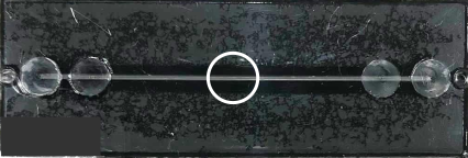
(a) Straight channel

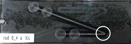
(b) Variation 3

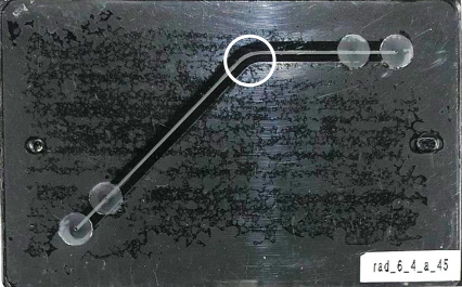
(c) Variation 1

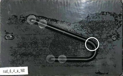
(d) Variation 2

Figure 3: Top view of milled microchannels with different geometries and their region of interest (ROI) marked as circle.

Figure 4: Schematic illustration of the angle $\beta$ (green), the outside radius ($R_{o}$) and inside radius ($R_{i}$) of the curved part of the example of variation 3.

Microchannel	$\beta$	$R_{o}$	$R_{i}$	$R_{o}/R_{i}$
	(deg)	($\text{\,}\mathrm{m}\mathrm{m}$)	($\text{\,}\mathrm{m}\mathrm{m}$)
Variation 1	45	6.68	6.12	1.09
Variation 2	160	6.68	6.12	1.09
Variation 3	160	0.68	0.12	5.23

Table 1: The angle of curved segment $\beta$, outside radius $R_{o}$, inside radius $R_{i}$ of the curved part of microchannels, and their ratio $R_{o}/R_{i}$.

As working fluid, de-ionized water and 50 wt% Glycerin/water mixture are used. To enhance the visibility, Fluorescin with a molar concentration of $5\text{\times}{10}^{-5}\text{\,}\mathrm{m}\mathrm{o}\mathrm{l}\mathrm{/}\mathrm{L}$ is added, ensuring not to influence the fluid physical properties. The density, the dynamic viscosity and the surface tension were internally determined and are given in table 2. It should be mentioned that the 50 wt% Glycerin/water mixture is applied only on the straight channel (fig. 3(a)), while water is applied for all three curved channels due to its relevance to the industrial applications.

Table 2: Physical properties of the working fluids and surface tension with air.

Working fluid	density	dyn. viscosity	surface tension
@ 22°C	$\rho\ ($\text{\,}\mathrm{k}\mathrm{g}\mathrm{/}\mathrm{m}^{3}$)$	$\mu\ ($\text{\,}\mathrm{P}\mathrm{a}\cdot\mathrm{s}$)$	$\sigma\ ($\text{\,}\mathrm{N}\mathrm{/}\mathrm{m}$)$
Water	998.03	1.000e-3	72.74e-3
50 wt% Glycerin/water mixture	1142	8.026e-3	68.12e-3

3.2 Experimental setup

Figure 5 shows the experimental setup of the whole test bench on the left side and a zoom-in view on the right side. The liquid flow is controlled by a syringe pump (CETONI Nemesys S). To clearly visualize the interface motion a FITC-Fluorescence setup in combination with a high-speed camera (NX4-S3, LDT) is used. Therefore, a high power LED is chosen (SOLIC-3C) as light source. To strictly define the excitation light spectrum an excitation filter is used (483x31$\text{\,}\mathrm{n}\mathrm{m}$). The filtered light beam is reflected on a dichroic mirror (refl.: 470 - 490$\text{\,}\mathrm{n}\mathrm{m}$, trans: 505 - 800$\text{\,}\mathrm{n}\mathrm{m}$) and excites the FITC molecules in the working fluid. The illuminated areas at the sample is marked with a circle in fig. 3. The phase-shifted emitted light is then transmitted through the dichroic mirror to the camera again. To remove possible effects by ambient light and reflections due to the emission beam an emission filter is included in the camera tubing system with a transmission spectrum of 530 $\times$ 45$\text{\,}\mathrm{n}\mathrm{m}$.

The ROI is visualized by 1024x1024 pixels with a resolution of $\Delta x=$6.566\text{\times}{10}^{-6}\text{\,}\mathrm{m}$$. The frame rate was chosen in dependency of the operation point and the flow rate (table 3). The image grabbing is accomplished with the software MotionStudio.

Figure 5: Experimental setup. Left: test bench. Right: zoom-in view with region of interest (ROI).

Table 3: Investigated volumetric flow rates, flow velocities in experiments and the corresponding optical frame rates.

Volumetric flow rate	Flow velocity	Frame rate
$\dot{V}\ (${10}^{-9}\text{\,}\mathrm{m}^{3}\mathrm{/}\mathrm{s}$)$	$U\ (${10}^{-3}\text{\,}\mathrm{m}\mathrm{/}\mathrm{s}$)$	(fps)
0.025, 0.11	0.11, 0.49	30
0.25, 0.67	1.11, 2.98	60
1.1, 1.8	4.89, 8.00	100
2.5	11.11	200
2.7, 3.1, 3.6, 4, 4.5	12.22, 13.78, 16.00, 17.78, 20.00	300

3.3 Experimental procedure

For all operation points a constant flow rate was chosen as listed in table 3. The liquid enters the channel at the inlet port and leaves the system via the outlet port (fig. 2). The image recording was manually started. The determination of the dynamic CA was done afterwards using the post-processing procedure, as described in section 4. After each test, the channel is cleaned with de-ionized water flow and then dried with air flow for 5 minutes.

To further characterize the liquid-solid-interaction the static CA was determined for every specific sample in addition. Therefore, the working fluid was pumped into the channel with the smallest volumetric flow rate $\dot{V}=$0.025\text{\times}{10}^{-9}\text{\,}\mathrm{m}^{3}\mathrm{/}\mathrm{s}$$ up to the middle of the ROI. Then, the pump was stopped and after a waiting time of three minutes the images were recorded for the static CA measurements. It should be noted due to the optical effect of sharp edges of the rectangular channel cross section and the limitation of 2D top-down visualization of the 3D fluid interface, the static CA values measured in channel can deviate from the values measured with a fluid droplet on a solid substrate. Nevertheless, the rivulet effect along sharp corner in rectangular channel is not relevant here as explained in appendix A.

4 Automated dynamic contact angle analysis

In this section, the proposed automated dynamic contact angle analysis is explained in four steps: interface detection (section 4.1), contact angle measurement (section 4.2), outlier removal (section 4.3) and output (section 4.4). The developed image processing procedure provides a technique for automated and robust measurement of the interfacial characteristics through microchannels with arbitrary geometries. This method is particularly advantageous for experiments with non-transparent samples, where extracting interface characteristics poses a challenge. The source code version used in this manuscript is archived in a jupyter notebook on GitHub [25].

Figure 6: Flow chart of automated image processing procedure: input (gray), interface detection (green), contact angle measurement (blue), outlier removal (red) and output (yellow).

4.1 Interface detection

To enable the contact angle measurements between interface and walls, the fluid interface need to be firstly identified and extracted. Figure 6 illustrates the sequential workflow of the automated image processing used in this work. Figure 7 provides an visual overview of the interface detection procedure with two successive images as examples. To optimize space utilization, only the first two pre-processed images are presented in their original size, while the subsequent images have been cropped for conciseness.

The complete contours of the fluid flow of two successive images at $t_{n}$ and $t_{n+1}$ are extracted as $c_{n}$ (fig. 7(c)) and $c_{n+1}$ (fig. 7(d)). Then the contour difference $c_{d}$ between $c_{n}$ and $c_{n+1}$ is calculated as $c_{d}=c_{n+1}-c_{n}$ (fig. 7(e)) with the momentum center as point $C(C_{x},C_{y})$ with $C_{x}=M_{10}/M_{00}$ and $C_{y}=M_{01}/M_{00}$ as shown in fig. 7(f). Here, $M=\sum_{x}\sum_{y}x^{i}y^{j}I(x,y)$ denotes the momentum of the contour difference $c_{d}$ with the $I(x,y)$ for the intensity of each pixel. To enable the subsequent iterations for interface detection, the closest point on the contour $c_{n}$ to the momentum center $C$ is found as the start point and is drawn in fig. 7(g) as the point $P$. From the point $P$, the iteration starts to search for the first two ”overlapping” points $a_{n}$ and $b_{n}$ (fig. 7(h)) of contour $c_{n}$ and $c_{n+1}$, which should be the boundary points of the interface of contour $c_{n}$. It should be emphasized that the “overlapping” here signifies the distance between two points smaller than a threshold value, which is given as a predefined parameter by the user. With the detected boundary points $a_{n}$ and $b_{n}$, the interface contour of image at $t_{n}$ can be obtained as shown in fig. 7(i).

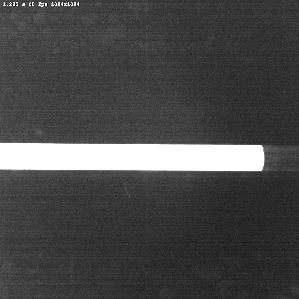
(a) Pre-processed image at $t_{n}$.

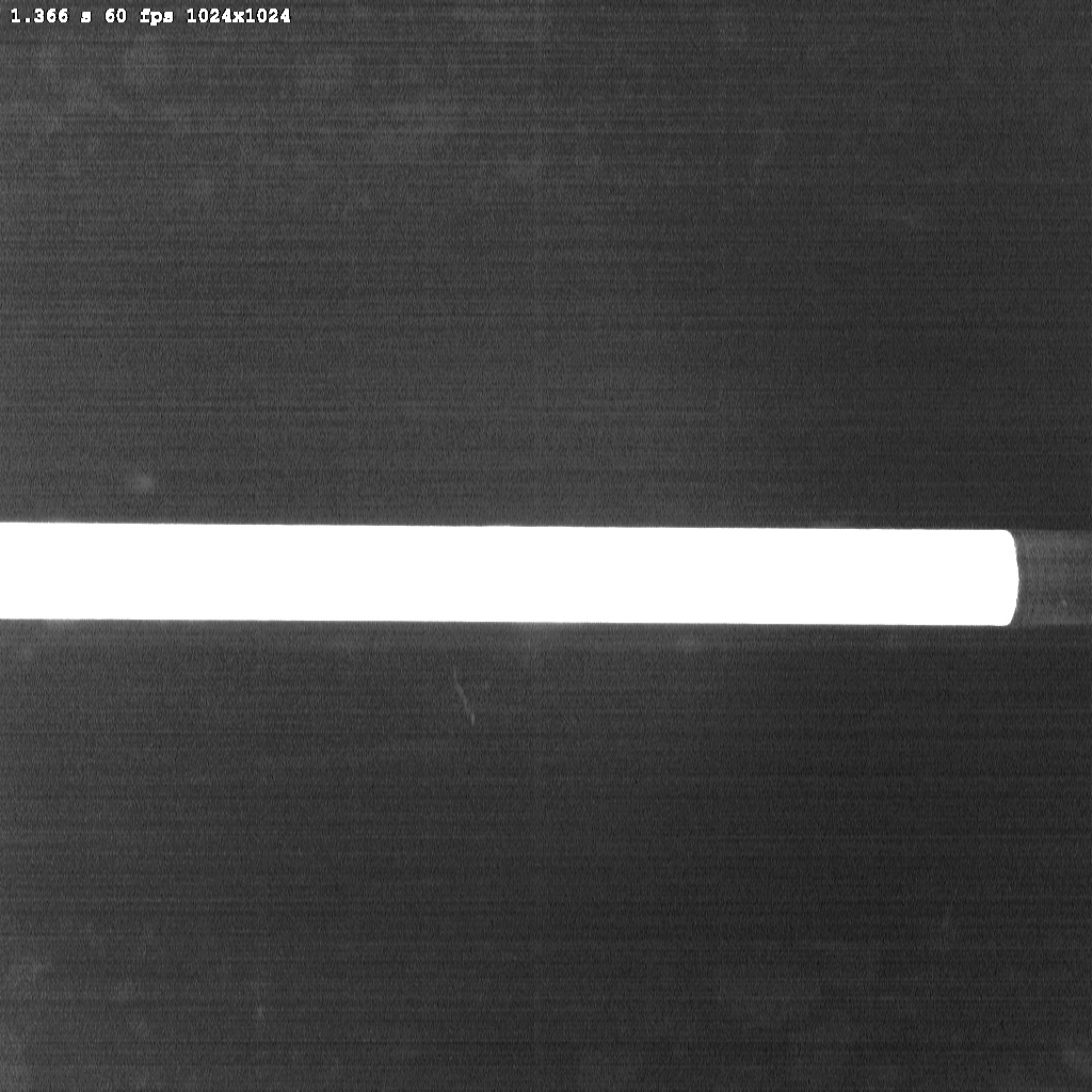
(b) Pre-processed image at $t_{n+1}$.

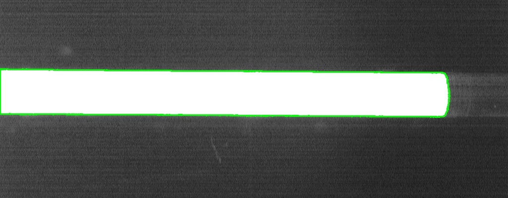
(c) Complete contour of the image at $t_{n}$ as $c_{n}$.

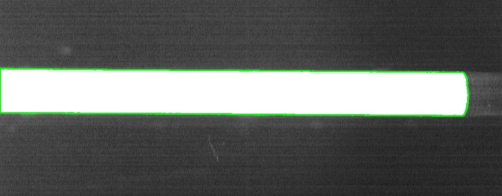
(d) Complete contour of the image at $t_{n+1}$ as $c_{n+1}$.

(e) Contour difference $c_{d}$ between $c_{n}$ and $c_{n+1}$.

(f) The momentum center $C$ (red point) of the contour difference $c_{d}$.

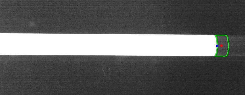
(g) The start point $P$ of the following iterations (blue point).

(h) The boundary points of the interface $a_{n}$ (blue point on top) and $b_{n}$ (blue point on bottom).

(i) The interface of the image at $t_{n}$.

Figure 7: The interface detection procedure.

4.2 Contact angle measurement

To measure the contact angle, the local tangents at boundary points $a_{n}$ and $b_{n}$ are identified in this proposed method. To derive these tangents, the algorithm selects the closest N pixels along the contour $c_{n}$ originating from the boundary points $a_{n}$ and $b_{n}$ (fig. 8(a)). The contact angle is subsequently calculated as the angle between the two selected tangents as presented in fig. 8(b).

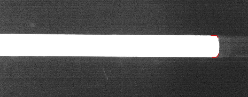
(a) Local tangents at boundary points $a_{n}$ and $b_{n}$ with the closest 10 pixels.

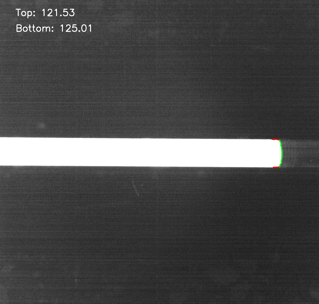
(b) Calculated contact angles displayed on the image.

Figure 8: Dynamic contact angle measurement procedure.

4.3 Outlier removal

Due to a small variance of the image qualities, the outlier removal is provided with two options in an intuitive way: channel width constraint and contact angle constraint. This step provides flexibility in addressing variations in data quality and ensures a more robust analysis.

Channel width constraint

The distance between the boundary points $a_{n}$ and $b_{n}$ should be equal to the microchannel width, which can be measured using microscope or camera precisely. Therefore, the microchannel width with a user pre-defined tolerance can be used as a criterion for the outlier removal.

Contact angle constraint

Knowing the static contact angle by previous experiments and the volumetric flow rate range allows the usage of a user defined reasonable contact angle range as the outlier removal criterion.

4.4 Output

The processed images with the detected interface and the corresponding contact angle information are saved in a new directory with the same file name as the original images. The interface movement is calculated using the image resolution and frame rate information, and then saved with the contact angle together in a CSV file. In addition, the temporal evolution of the meniscus displacement and dynamic contact angle can be visualized as plots.

To utilize the procedure for further analysis, the algorithm is firstly validated in section 5.1. Its automation through Python not only enhances efficiency, significantly reducing processing time, but also facilitates direct comparisons to manually measured data, thereby ensuring the method’s validity and reliability. However, this method might not be suitable for images with either substantial or minimal differences, for example, images taken with extremely low or high frame rates, which could lead to less reliable results. The exceedingly fast frame rates might cause the interface difference between two subsequent images too small to be detected by the algorithm, while the slow frame rates can result in the interface moving away too significantly from its previous position, thereby causing higher uncertainty in the detection of interface boundary points. Therefore, validation on a test set of images from an experiment is necessary to set the sampling rate of recorded images before applying the algorithm.

5 Results and discussion

5.1 Validation of automated analysis

Interface detection

A correct interface detection procedure (section 4.1) is fundamental for the accuracy of the automated dynamic contact angle (CA) analysis. The interface velocity is selected to be the validation parameter as a consequence of the volumetric flow rate controlled flow by the syringe pump. The theoretical interface velocity $U_{theo}=\dot{V}/A$ can be calculated using the cross section dimension of microchannels measured using a microscope. As mentioned in section 4.4, the temporal evolution of the meniscus displacement (top and bottom) is obtained as output, of which the mean value can be further analyzed for the interface velocity $U_{code}=(x_{n}-x_{0})/(t_{n}-t_{0})$. The comparison between the theoretical and measured interface velocity in the form of velocity error $|U_{theo}-U_{code}|/U_{theo}$ of all tested flow rates is summarized as violin plots in fig. 9. It is clearly visible that the algorithm captures the moving interface of serial images precisely with the maximum velocity error below 5% and the mean velocity error smaller than 3%.

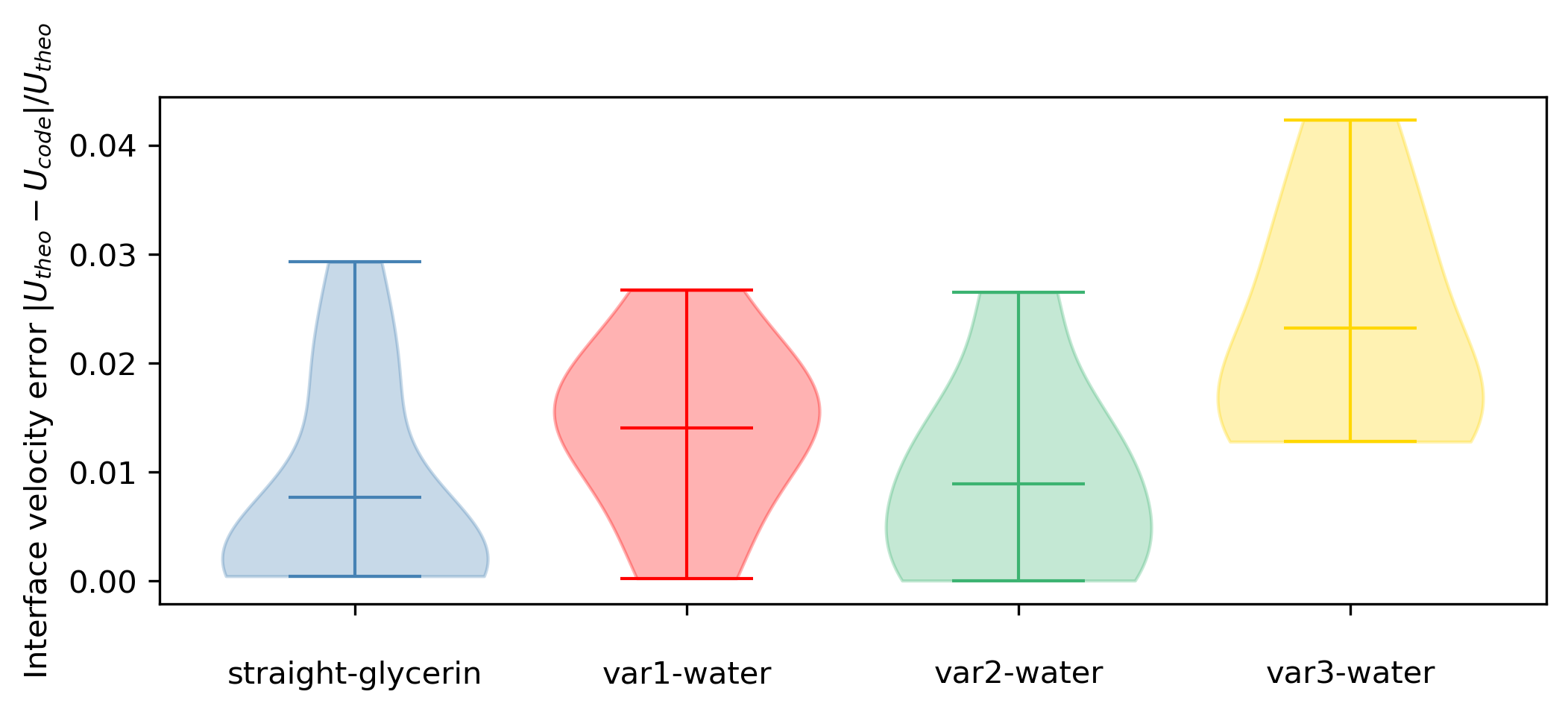
Figure 9: Comparison of theoretical interface velocity $U_{theo}$ and calculated interface velocity from measurements $U_{code}$ for interface detection validation as violin plots. Top line: maximum. Middle line: mean. Bottom line: minimum.

Contact angle measurement

The automated dynamic CA measurement via local tangents is validated here by comparison with the manually measured results. To ensure the reproducibility and reliability of the manual data, three random images of each test are chosen and the CAs at both channel sides of each image are measured three times with [18], respectively, of which the average value is then picked to be the manually measured as dynamic CA $\theta_{manual}$. As explained in section 4.2, the number of the closest pixels for the local tangents is chosen to be $N=10$ for the dynamic CA calculation $\theta_{code}$. Figure 10 summarizes the results of all considered flow rates (table 3) as violin plots. The violin plots reveal that the results from the algorithm are quite comparable to the manual measurements and the CA error $|\theta_{manual}-\theta_{code}|/\theta_{manual}$ for all tests is below 2%.

Based on the above validation, all experimental results shown in the following sections refer to the data from the automated analysis.

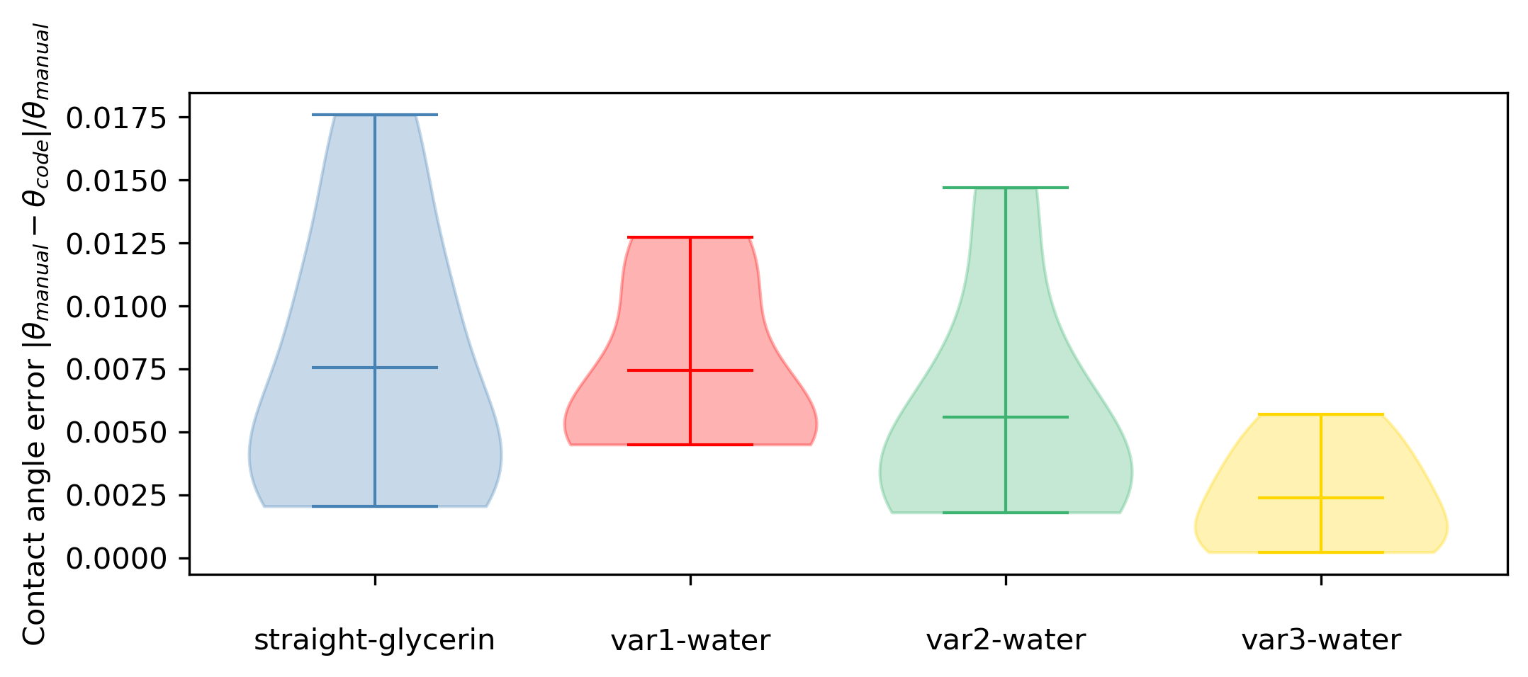
Figure 10: Comparison of dynamic contact angle from manual measurements $\theta_{manual}$ and automated measurements $\theta_{code}$ as violin plots with case-variant distribution. Top line: maximum. Middle line: mean. Bottom line: minimum.

5.2 Molecular Kinetic Theory

As stated in section 2, the MKT is utilized as the theoretical analysis for fitting the experimental results from the forced wetting through various microchannels. Figure 11 depicts the experimental dynamic CA $\theta_{d}$ versus the capillary number $\mathit{Ca}$ for 50 wt% Glycerin/water mixture through the straight channel and water through three curved channels. The static CA $\theta_{0}$ and the values for the fitting parameters are summarized in table 4, whose orders of magnitude are physically reasonable (see section 2). Despite the curved parts of the microchannel variation 1 and variation 2, their curvature ratio $R_{o}/R_{i}=1.09$ is small and could be utilized directly for the comparison with straight channel. Nevertheless, the curved part of variation 3 with $R_{o}/R_{i}=5.29$ could not be ignored, which results in the extraction of the experimental data from the straight part (fig. 12(a)) of variation 3 for the further analysis.

For both working fluids, the measured dynamic CA matches well with the MKT theory, meaning the advancing dynamic CA increases with larger capillary number. That confirms the MKT’s suitability for describing the CL dynamics of forced wetting through straight microchannels, not only limited by the conventional experimental methods (for example, Wilhelmy plate investigated by [20]). What stands out in table 4 is the increase of $\kappa^{0}$ with more viscous fluid. That indicates that the molecules of more viscous fluid tend to attach and detach faster than less viscous fluid, which appears counter-intuitive. According to the definition of the equilibrium frequency in section 2, the different $\kappa^{0}$ could be related to, for example, the fluid viscosity and the friction coefficient affected by the local roughness ([9]; [14]).

Extending the forced flow investigation through the straight channel to three more different microchannels, as introduced in fig. 3, the scope of the MKT’s appropriateness for forced wetting could be broadened. It can be seen that the measured dynamic CAs depend on the channel geometry. For each geometry, a separate curve-fitting is performed and the obtained parameters are given in table 4. Interestingly, even with the same working fluid, the equilibrium frequency $\kappa^{0}$ varies from $11.94\text{\,}\mathrm{k}\mathrm{H}\mathrm{z}$ to $756.56\text{\,}\mathrm{k}\mathrm{H}\mathrm{z}$, which might be attributed to the different surface roughness of the samples, for example, the tool abrasion and different milling speeds along the curved region during the manufacturing may have led to different roughness in the samples.

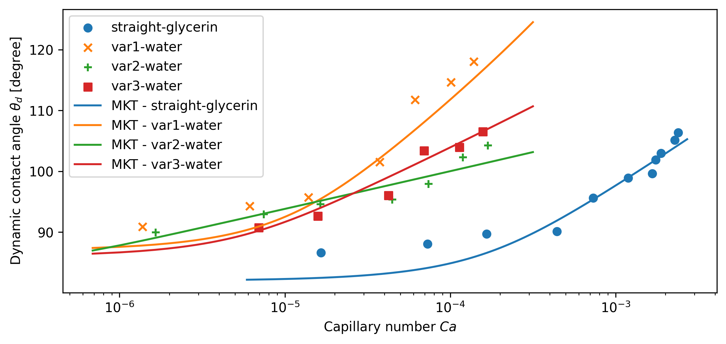
Figure 11: Dynamic contact angle $\theta_{d}$ versus the capillary number $\mathit{Ca}$ for 50 wt% Glycerin/water mixture through straight channel and water through three curved microchannels.

Table 4: The static contact angle and the MKT parameters estimated from curve-fitting analysis for 50 wt% Glycerin/water mixture through straight channel and water through three curved microchannels.

Microchannel - Fluid	$\theta_{0}$	$\lambda$	$\kappa^{0}$
	(deg)	($\text{\,}\mathrm{n}\mathrm{m}$)	($\text{\,}\mathrm{k}\mathrm{H}\mathrm{z}$)
Straight - 50% Glycerin-water	91	1.09	60.6
Variation 1 - Water	87	0.81	756.56
Variation 2 - Water	84	1.55	11.94
Variation 3 - Water	86	1.07	284.86

5.3 Influence of curved microchannel on the dynamic contact angle

Now that the MKT’s suitability is confirmed by two working fluids and four different microchannels, the performance of MKT with forced flow through microchannel with large curvature ratio is further studied.

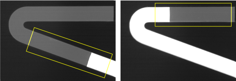
(a) Straight part (yellow). Left: $t=$0.983\text{\,}\mathrm{s}$$. Right: $t=$10.716\text{\,}\mathrm{s}$$.

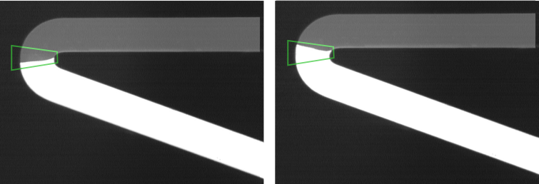
(b) Position 1 (green). Left: $t=$7.516\text{\,}\mathrm{s}$$. Right: $t=$7.783\text{\,}\mathrm{s}$$.

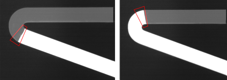
(c) Position 2 (red). Left: $t=$6.716\text{\,}\mathrm{s}$$. Right: $t=$8.850\text{\,}\mathrm{s}$$.

Figure 12: The microchannel variation 3 is classified as three parts ($\dot{V}=$0.000\,11\text{\,}\mathrm{m}\mathrm{L}\mathrm{/}\mathrm{s}$$): (a) straight part (yellow), (b) position 1 (blue) and (c) position 2 (red).

To study how the curved part will affect the dynamic wetting behavior, the microchannel variation 3 is divided into two parts: straight part (fig. 12(a)) and curved part, while the curved part is further classified as position 1 (fig. 12(b)) and position 2 (fig. 12(c)) for the reason of exhibiting different wetting behaviors. The position 1 refers to the middle of the curved part, while the position 2 covers the begin and the end. Owing to the large curvature ratio $R_{o}/R_{i}=5.29$, the dynamic CAs of curved part are measured at inside and outside, respectively. Having the information of inside radius $R_{i}$, outside radius $R_{o}$ (table 1) and the flow velocity allows the calculations of local CL velocities at the inside and the outside of curved parts.

Plotting the dynamic CA $\theta_{d}$ with $\mathit{Ca}$ calculated using local CL velocities, the comparison between experimental results and fit to the MKT model can be seen in fig. 13. The free parameters $\kappa^{0}$ and $\lambda$ estimated from curve-fitting are listed in table 5. It should be noted that the identical static CA $\theta_{0}=86$° is employed for all parts of variation 3, except for the inside of position 1, where $\theta_{0}=70$° is applied. That is attributed to the observed significantly small dynamic CAs, resulting from the formation of a distinct tip between the interface and the wall as presented in fig. 12(b). This strong bending of interface along the inside CL is mostly likely due to the considerable difference of the local CL velocities between the inner and the outer radius of the microchannel, causing the pinning of the inner radius CL. The different shear rates on curved region might also contribute to this phenomenon. In addition, it is worth stressing that the rectangular geometry of a channel is known to cause the “finger” effect of the CL along the sharp edges of channel ([10]; [34]), which might be enhanced by the pronounced curvature of variation 3.

As a consequence of the smaller dynamic CA at the inside of position 1 than the measured static CA $\theta_{0}=86$°, a derived static CA $\theta_{0}=70$° from the previous results is utilized for the inside of position 1. As shown in fig. 13, the dynamic wetting behavior of water through variation 3 could be well interpreted using MKT, with the obtained parameters (table 5) not only physically meaningful, but also lay in a similar range. Again, the suitability of the MKT approach to describe the CL dynamics of forced wetting through microchannels is confirmed, even in scenarios involving geometrically complex microchannels. The dynamic CA depends not only on the channel geometry, but also significantly on the curvature ratio.

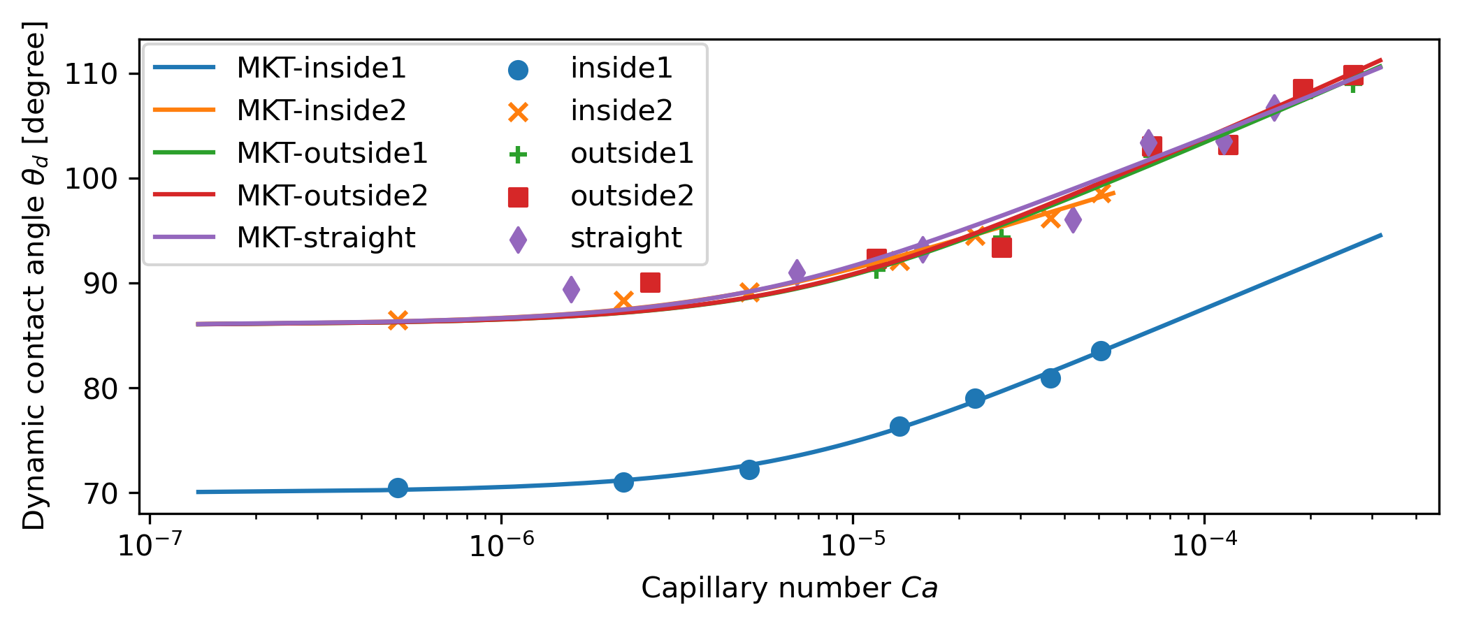
Figure 13: Dynamic contact angle $\theta_{d}$ versus capillary number $\mathit{Ca}$ with water through three parts of variation 3: straight part, position 1 and position 2.

Table 5: The static contact angle and the MKT parameters estimated from curve-fitting analysis for forced wetting through three parts of variation 3 with water.

Channel part	$\theta_{0}$ (deg)	$\lambda$ ($\text{\,}\mathrm{n}\mathrm{m}$)	$\kappa^{0}$ ($\text{\,}\mathrm{k}\mathrm{H}\mathrm{z}$)
Straight	86	1.07	284.86
Inside position 1	70	1.03	424.12
Outside position 1	86	1.03	400.75
Inside position 2	86	1.20	195.86
Outside position 2	86	1.02	410.16

6 Conclusions and Outlook

To gain a better understanding of the sealing issue in industrial products, where the leakage pots are prone to posses rough surface and complex geometries, an appropriate dynamic contact angle (CA) model is crucial. In present work, the dynamic wetting behaviors of forced flow with small capillary number $\mathit{Ca}$ ($10^{-6}$ - $10^{-3}$) through geometrically complex microchannels are investigated experimentally, to cover the most common leaking circumstances in application. In addition to the industrial most relevant fluid - water, 50 wt% Glycerin/water mixture is employed to examine the suitability of MKT approach. The forced wetting through three curved microchannels with different geometry and curvature ratio $R_{o}/R_{i}$ is conducted and the findings confirm again the feasibility of applying the MKT on the CL dynamics involved in industrial circumstances, meaning not only the flow through microchannels with rough surface, but also with geometrical complexity. The channel geometry as well as the significantly different curvatures of curved microchannels have influence on the CL movement. However, the deviation of the free parameter $\kappa^{0}$ between different experiments is still not clear. The other phenomenon need to be further explored is the extremely small dynamic CAs appearing on the inside of the position 1 of variation 3. More studies are suggested to include curved channels with ratios between 1.09 and 5.23, so that the pinning effect on this position could be further accompanied by numerical simulations to investigate the flow fields near the inner CL.

Moreover, the proposed automated image analysis for dynamic CA measurement provides a straightforward and reliable means to systematically analyze the interface movement within images acquired from non-transparent samples, meaning the interface could not be extracted easily. It not only offers simplicity in its application but significantly reduces the time invested in manual measurements.

The presented experimental results will serve as a basis for the further 3D transient numerical investigations of dynamic wetting behaviors to compliment the 2D experimental results and cover a more broad spectrum of industrial media tightness topic.

7 Acknowledgments

The authors would like to thank Prof. Dr. Joël De Coninck of Université libre de Bruxelles for the helpful and valuable discussion on the experimental results. The last two authors acknowledge the funding by the German Research Foundation (DFG): July 1 2020 - 30 June 2024 funded by the German Research Foundation (DFG) - Project-ID 265191195 - SFB 1194.

Appendix A Appendix: Rectangular channel geometry and corner fluid rivulet

In fig. 14 the microscopy of the cross-section of the straight channel (fig. 3(a)) is displayed, showing the exact channel dimension of the chosen position and the sharp edge of the channel by micromilling.

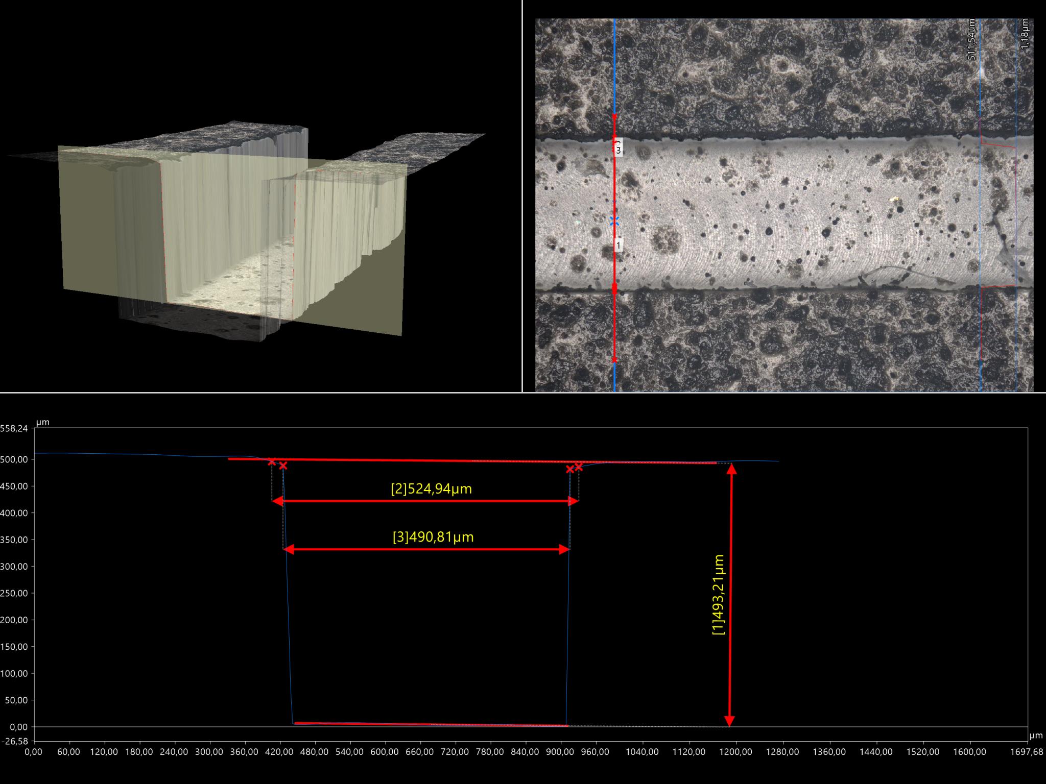
Figure 14: Microscopy of the straight channel cross-section. Top left: depth profile of the chosen section of straight channel. Top right: top view of the chosen-section and the chose position for measurements (blue line). Bottom: depth profile of the chosen position and measurements (red line).

Figure 15: Simulation result in Surface Evolver with three PMMA walls ($\theta_{0}=80$°) and one TPU wall ($\theta_{0}=104$°). Below the interface is water while above the interface is air. Left: side view. Right: top view.

It is well-known that the wetting in a rectangular channel leads to rivulets along the sharp corner ([19]; [30]), however, [7] found that for the wetting cases with an equilibrium contact angle $\theta_{0}>45$°, there are no rivulets. Employing the 3D Surface Evolver [4] as an addition source for the microchannel with three PMMA walls ($\theta_{0}=80$°) and one TPU wall ($\theta_{0}=104$°), the resolved interface in channel with the exact 2D top-down view as in experiment is given in fig. 15. With no visible corner rivulet in fig. 15, it can be said that the results obtained with a 2D top-down view from experiments are not affected by rivulets.

References

- \bibcommenthead
- Blake and Haynes [1969] Blake, T.D., Haynes, J.M.: Kinetics of liquidliquid displacement. Journal of Colloid and Interface Science 30(3), 421–423 (1969) https://doi.org/10.1016/0021-9797(69)90411-1
- Blake [1993] Blake, T.D.: Dynamic contact angle and wetting kinetics. Wettability (1993)
- Blake [2006] Blake, T.D.: The physics of moving wetting lines. Journal of Colloid and Interface Science 299(1), 1–13 (2006) https://doi.org/10.1016/j.jcis.2006.03.051
- Brakke [1992] Brakke, K.A.: The surface evolver. Experimental Mathematics 1(2), 141–165 (1992) https://doi.org/10.1080/10586458.1992.10504253 https://doi.org/10.1080/10586458.1992.10504253
- Brochard-Wyart and de Gennes [1992] Brochard-Wyart, F., de Gennes, P.G.: Dynamics of partial wetting. Advances in Colloid and Interface Science 39, 1–11 (1992) https://doi.org/10.1016/0001-8686(92)80052-Y
- Chen et al. [2017] Chen, X., Chen, J., Ouyang, X., Song, Y., Xu, R., Jiang, P.: Water droplet spreading and wicking on nanostructured surfaces. Langmuir 33(27), 6701–6707 (2017) https://doi.org/%****␣sn-article.bbl␣Line␣125␣****10.1021/acs.langmuir.7b01223 https://doi.org/10.1021/acs.langmuir.7b01223. PMID: 28609626
- Concus and Finn [1969] Concus, P., Finn, R.: On the behavior of a capillary surface in a wedge¡sup¿*¡/sup¿. Proceedings of the National Academy of Sciences 63(2), 292–299 (1969) https://doi.org/10.1073/pnas.63.2.292 https://www.pnas.org/doi/pdf/10.1073/pnas.63.2.292
- Clanet and Quéré [2002] Clanet, C., Quéré, D.: Onset of menisci. Journal of Fluid Mechanics 460, 131–149 (2002) https://doi.org/10.1017/S002211200200808X
- Duvivier et al. [2013] Duvivier, D., Blake, T.D., De Coninck, J.: Toward a predictive theory of wetting dynamics. Langmuir 29(32), 10132–10140 (2013) https://doi.org/10.1021/la4017917 https://doi.org/10.1021/la4017917. PMID: 23844877
- Dong and Chatzis [1995] Dong, M., Chatzis, I.: The imbibition and flow of a wetting liquid along the corners of a square capillary tube. Journal of Colloid and Interface Science 172(2), 278–288 (1995) https://doi.org/10.1006/jcis.1995.1253
- de Gennes [1985] Gennes, P.G.: Wetting: statics and dynamics. Rev. Mod. Phys. 57, 827–863 (1985) https://doi.org/%****␣sn-article.bbl␣Line␣200␣****10.1103/RevModPhys.57.827
- de Ruijter et al. [1999] Ruijter, M.J., Blake, T.D., De Coninck, J.: Dynamic wetting studied by molecular modeling simulations of droplet spreading. Langmuir 15(22), 7836–7847 (1999) https://doi.org/10.1021/la990171l https://doi.org/10.1021/la990171l
- de Ruiter et al. [2017] Ruiter, R., Colinet, P., Brunet, P., Snoeijer, J.H., Gelderblom, H.: Contact line arrest in solidifying spreading drops. Phys. Rev. Fluids 2, 043602 (2017) https://doi.org/10.1103/PhysRevFluids.2.043602
- Duvivier et al. [2011] Duvivier, D., Seveno, D., Rioboo, R., Blake, T.D., De Coninck, J.: Experimental evidence of the role of viscosity in the molecular kinetic theory of dynamic wetting. Langmuir 27(21), 13015–13021 (2011) https://doi.org/%****␣sn-article.bbl␣Line␣250␣****10.1021/la202836q https://doi.org/10.1021/la202836q. PMID: 21919445
- Eddi et al. [2013] Eddi, A., Winkels, K.G., Snoeijer, J.H.: Short time dynamics of viscous drop spreading. Physics of Fluids 25(1) (2013) https://doi.org/10.1063/1.4788693 . Cited by: 130; All Open Access, Green Open Access
- Hygum and Popok [2015] Hygum, M., Popok, V.: Modeling of humidity-related reliability in enclosures with electronics. In: Kutilainen, J. (ed.) IMAPS Nordic Annual Conference 2015 June 8-9, Helsingør, pp. 106–110. Curran Associates, Inc, ??? (2015). IMAPS Nordic 2015 Conference : International Microelectronics And Packaging Society ; Conference date: 01-07-2015
- Huh and Scriven [1971] Huh, C., Scriven, L.E.: Hydrodynamic model of steady movement of a solid/liquid/fluid contact line. Journal of Colloid and Interface Science 35(1), 85–101 (1971) https://doi.org/10.1016/0021-9797(71)90188-3
- ImageJ [2023] ImageJ: Image Processing and Analysis in Java (2023). https://imagej.net/ij/
- Kubochkin and Gambaryan-Roisman [2022] Kubochkin, N., Gambaryan-Roisman, T.: Capillary-driven flow in corner geometries. Current Opinion in Colloid & Interface Science 59, 101575 (2022) https://doi.org/10.1016/j.cocis.2022.101575
- Mohammad Karim [2022] Mohammad Karim, A.: A review of physics of moving contact line dynamics models and its applications in interfacial science. Journal of Applied Physics 132(8), 080701 (2022) https://doi.org/10.1063/5.0102028 https://pubs.aip.org/aip/jap/article-pdf/doi/10.1063/5.0102028/16511412/080701_1_online.pdf
- Mohammad Karim et al. [2016] Mohammad Karim, A., Davis, S.H., Kavehpour, H.P.: Forced versus spontaneous spreading of liquids. Langmuir 32(40), 10153–10158 (2016) https://doi.org/10.1021/acs.langmuir.6b00747 https://doi.org/10.1021/acs.langmuir.6b00747. PMID: 27643428
- Malkiel and Rabinovitch [2023] Malkiel, N., Rabinovitch, O.: Stochastic delamination processes – a comparative analysis. International Journal of Solids and Structures 267, 112159 (2023) https://doi.org/10.1016/j.ijsolstr.2023.112159
- Mohammad Karim et al. [2018] Mohammad Karim, A., Rothstein, J.P., Kavehpour, H.P.: Experimental study of dynamic contact angles on rough hydrophobic surfaces. Journal of Colloid and Interface Science 513, 658–665 (2018) https://doi.org/10.1016/j.jcis.2017.11.075
- Petrov and Petrov [1992] Petrov, P., Petrov, I.: A combined molecular-hydrodynamic approach to wetting kinetics. Langmuir 8(7), 1762–1767 (1992) https://doi.org/10.1021/la00043a013 https://doi.org/10.1021/la00043a013
- Robert Bosch GmbH [2024] Robert Bosch GmbH: BoschResearch/sepMutliphaseFoam, git tree/publications/automatedImageAnalysisForInterfaceTrackingInCurvedChannels. https://github.com/boschresearch/sepMultiphaseFoam/tree/publications/automatedImageAnalysisForInterfaceTrackingInCurvedChannels. Created: 2024-03-14 (2024)
- Sedev [2015] Sedev, R.: The molecular-kinetic approach to wetting dynamics: Achievements and limitations. Advances in Colloid and Interface Science 222, 661–669 (2015) https://doi.org/10.1016/j.cis.2014.09.008 . Reinhard Miller, Honorary Issue
- Seveno [2005] Seveno, D.: Dynamic wetting of fibers/mouillage dynamique des fibres (2005)
- Shikhmurzaev [1993] Shikhmurzaev, Y.D.: The moving contact line on a smooth solid surface. International Journal of Multiphase Flow 19(4), 589–610 (1993) https://doi.org/10.1016/0301-9322(93)90090-H
- Sauer and Kampert [1998] Sauer, B.B., Kampert, W.G.: Influence of viscosity on forced and spontaneous spreading: Wilhelmy fiber studies including practical methods for rapid viscosity measurement. Journal of Colloid and Interface Science 199(1), 28–37 (1998) https://doi.org/10.1006/jcis.1997.5319
- Thammanna Gurumurthy et al. [2022] Thammanna Gurumurthy, V., Baumhauer, M., Khair, A., Roisman, I.V., Tropea, C., Garoff, S.: Forced wetting in a square capillary. Phys. Rev. Fluids 7, 114002 (2022) https://doi.org/10.1103/PhysRevFluids.7.114002
- Voinov [1976] Voinov, O.V.: Hydrodynamics of wetting. Fluid Dynamics 11, 714–721 (1976)
- Vega et al. [2005] Vega, M.-J., Seveno, D., Lemaur, G., Adão, M.-H., De Coninck, J.: Dynamics of the rise around a fiber: Experimental evidence of the existence of several time scales. Langmuir 21(21), 9584–9590 (2005) https://doi.org/10.1021/la051341z https://doi.org/10.1021/la051341z. PMID: 16207039
- Wang et al. [2013] Wang, H., Liserre, M., Blaabjerg, F.: Toward reliable power electronics: Challenges, design tools, and opportunities. IEEE Industrial Electronics Magazine 7(2), 17–26 (2013) https://doi.org/10.1109/MIE.2013.2252958
- Wong et al. [1992] Wong, H., Morris, S., Radke, C.J.: Three-dimensional menisci in polygonal capillaries. Journal of Colloid and Interface Science 148(2), 317–336 (1992) https://doi.org/10.1016/0021-9797(92)90171-H
- Wang et al. [2016] Wang, X., Venzmer, J., Bonaccurso, E.: Surfactant-enhanced spreading of sessile water drops on polypropylene surfaces. Langmuir 32(33), 8322–8328 (2016) https://doi.org/%****␣sn-article.bbl␣Line␣550␣****10.1021/acs.langmuir.6b01357 https://doi.org/10.1021/acs.langmuir.6b01357. PMID: 27448154
- Zhang et al. [2023] Zhang, Y., Guo, M., Seveno, D., De Coninck, J.: Dynamic wetting of various liquids: Theoretical models, experiments, simulations and applications. Advances in Colloid and Interface Science 313, 102861 (2023) https://doi.org/10.1016/j.cis.2023.102861
- Zhang et al. [2024-03-13] Zhang, H., Lippert, A., Leonhardt, R., Tolle, T., Nagel, L., Fricke, M., Maric, T.: Experimental study of dynamic wetting behavior through curved microchannels with automated image analysis - Data. Technical University of Darmstadt (2024-03-13). https://tudatalib.ulb.tu-darmstadt.de/handle/tudatalib/4176