On Discrete Subproblems in Integer Optimal Control with Total Variation Regularization in Two Dimensions

Abstract

We analyze integer linear programs which we obtain after discretizing two-dimensional subproblems arising from a trust-region algorithm for mixed integer optimal control problems with total variation regularization. We discuss NP-hardness of the discretized problems and the connection to graph-based problems. We show that the underlying polyhedron exhibits structural restrictions in its vertices with regards to which variables can attain fractional values at the same time. Based on this property, we derive cutting planes by employing a relation to shortest-path and minimum bisection problems. We propose a branching rule and a primal heuristic which improves previously found feasible points. We validate the proposed tools with a numerical benchmark in a standard integer programming solver. We observe a significant speedup for medium-sized problems. Our results give hints for scaling towards larger instances in the future.

1 Introduction

We concern ourselves with problems of the form

$$\begin{aligned} \min_{d}\quad&\sum_{i=1}^{N}\sum_{j=1}^{M}c_{i,j}d_{i,j}+\alpha\sum_{j=1}^{M}\sum_{i=1}^{N-1}|x_{i+1,j}+d_{i+1,j}-x_{i,j}-d_{i,j}|\\ &+\alpha\sum_{i=1}^{N}\sum_{j=1}^{M-1}|x_{i,j+1}+d_{i,j+1}-x_{i,j}-d_{i,j}|\\ \text{s.t.}\quad&x_{i,j}+d_{i,j}\in\Xi\text{ for all }i\in[N],j\in[M],\\ &\sum_{i=1}^{N}\sum_{j=1}^{M}|d_{i,j}|\leq\Delta,\end{aligned}$$ (TR-IP)

where $N,M\in\mathbb{N}$, $x\in\Xi^{N\times M}$, $c\in\mathbb{R}^{N\times M}$, $\alpha>0$ and a finite set $\Xi\subset\mathbb{Z}$ are given. The problems (TR-IP) can be reformulated as integer (linear) programs and arise as trust-region subproblems in an algorithm for integer optimal control problems (IOCPs) with total variation penalization. Optimal control problems are optimization problems which are constrained by ordinary or partial differential equations. IOCPs additionally require the control function to only take integer values. Due to these constraints, IOCPs are a useful modelling approach with a variety of applications. The fields of application include, but are not limited to, the optimal control of solar thermal climate systems, see [7], aircraft trajectory planning, see [31], gas network control, see [18], and automotive control, see [14].

A popular approach to solve IOCPs is the combinatorial integral approximation (CIA) due to optimality guarantees of the approximation if certain conditions on the underlying differential equation are met, see [27]. This approach however does not restrict the switching of the control function values which can undermine the applicability of the found optimal solution. More details can be found in [17] and [4] and their references.

One approach to decrease the switching is to include the total variation of the control function into the problem formulation. In [6] the set of feasible controls is a bounded subset of functions with bounded variation. This allows for the construction of a branch-and-bound algorithm in order to solve parabolic optimal control problems with switching constraints, which include the aforementioned restriction but can be extended to include additional combinatorial constraints. Instead of using hard constraints one can instead introduce a total variation penalty in the objective to achieve a control with a lower switching frequency as done in e.g. [21] and [23]. In order to solve IOCP with total variation penalization the authors in [21] propose a trust-region method for which the arising discretized subproblems are modelled as integer (linear) programs. The convergence and optimality results are given for an underlying one-dimensional domain and thus one-dimensional subproblems. [22] consider the case of domains of dimension two and higher extending the result given in [21]. The computational bottleneck of the approach is the computational demand of the underlying integer programs, currently solved without structure exploitation with off-the-shelf solvers. For the one-dimensional case, a shortest path approach can be used to significantly reduce the run time of the algorithm, see [30]. In this paper we turn to the two-dimensional case, analyzing the resulting subproblems and proposing a series of improvements to the integer programming formulation and its solution process with a standard solver in order to reduce the computational demand. We highlight that the discretized problems are interesting beyond the intended application in integer optimal control. Specifically, similar problems can be found in image segmentation, see [5, 15], and multi-label optimization for Potts and Ising spin glass models, see [24, 10], but (TR-IP) contains additional constraints such that it can be viewed as minimum $s$-$t$ cut problem with a knapsack-type constraint.

Contribution

We provide structural results for the underlying polyhedrons of an integer programming reformulation of (TR-IP). We prove that the resulting problems are strongly NP-hard if the minimum bisection problem on subgraphs of the grid with an arbitrary number of holes is NP-hard. We extend our results in [30] and provide a conditional p-approximation for the integer programs. We prove that the vertices of the underlying polyhedron can only attain non-integer values in connected parts of a corresponding graph. For the binary case, we show that every feasible point of the integer program is already a vertex of the polyhedron which is false for the non-binary case. We employ our findings in an integer programming solver-based solution process. We derive cutting planes which make use of this property of the polyhedron as well as an approach to improve primal points and a branching rule. We validate the improvements with respect to the run time on a numerical benchmark example.

Structure of the remainder

We introduce the problem class in Section 2 and briefly restate the trust-region algorithm from [21]. We derive integer programs as reformulations of trust-region subproblems in Section 3. We discuss NP-hardness for the subproblem in Subsection 3.2. We introduce a Lagrangian relaxation in Subsection 3.3 and will analyze the connection to graph-based approaches, namely minimum $s$-$t$ cut problems, in Subsection 3.4. Afterwards we state and prove the aforementioned property of the underlying polyhedron in Section 4 which we then use to obtain cutting planes as well as primal points and a branching rule in Section 5. In the computational experiments in Section 6 we validate the proposed approaches and discuss the results and how to gauge the computational demand of the integer program in Section 7.

Notation

For convenience and improved visual clarity we use the short notation $[N]\coloneqq\{1,\ldots,N\}$. We introduce the notation $\lfloor x\rceil$ to represent the rounding of $x$ to the nearest integer value. In case of parity, $x$ is rounded up. The notation $\lceil x\rceil$ denotes rounding up to the nearest larger integer value while $\lfloor x\rfloor$ denotes rounding down.

In the paper we use the terminology polyhedron for which different definitions exist depending on the community. In our paper a polyhedron is the intersection of finitely many closed halfspaces.

2 Trust-region method for IOCPs

In this section we introduce the motivating class of IOCPs as well as the trust-region algorithm employed to solve the IOCPs. We will discretize its subproblems in the next section and concern ourselves with the resulting discrete problem in the remainder of this paper.

Let $\alpha>0$ and $\Omega\subset\mathbb{R}^{2}$ be a rectangular domain. The IOCP reads

$$\begin{aligned} &\min_{v\in L^{2}(\Omega)}J(v)\coloneqq F(v)+\alpha\operatorname*{TV}(v)\\ &\text{s.t. }v(x)\in\Xi\coloneqq\{\xi_{1},\ldots,\xi_{m}\}\subset\mathbb{Z}\text{ for almost all (a.a.) }x\in\Omega.\end{aligned}$$ (IOCP)

The function $F:L^{2}(\Omega)\mapsto\mathbb{R}$ is lower semicontinuous. The term $\operatorname*{TV}:L^{1}(\Omega)\to[0,\infty]$ denotes the total variation seminorm which models and penalizes the switching behaviour of the control function $v$. The set $\Xi$ contains all possible control values $\xi_{1},\ldots,\xi_{m}$ and thus enforces integrality of the control function values. In this paper we assume that $\Xi$ is a contiguous set of integers.

The trust-region algorithm described in [21] can be employed for problems of the form (IOCP). The pseudo code is given in Algorithm 1. The algorithm consists of one outer and one inner loop. The inner loop solves a trust-region subproblem

$$\begin{aligned} \min_{d\in L^{2}(\Omega)}&(\nabla F(v),d)_{L^{2}(\Omega)}+\alpha\operatorname*{TV}(v+d)-\alpha\operatorname*{TV}(v)\eqqcolon-pr(v,d)\\ \text{~{}~{}s.t.~{}~{}}&v(x)+d(x)\in\Xi\text{ for a.a.\ }x\in\Omega,\\ &\|d\|_{L^{1}(\Omega)}\leq\Delta\end{aligned}$$ (TR)

to obtain an optimal step in the trust region. If the predicted reduction $pr$ is zero the algorithm terminates. The underlying optimality results and assumptions can be found in [21] and [22]. If the predicted reduction is not zero it is checked if it exceeds a certain fraction of the actual reduction achieved by the solution to (TR). If yes, the calculated step is accepted and the inner loop is terminated. Otherwise, the step is rejected and the inner loop begins anew with a reduced trust-region radius. In the outer loop the trust-region radius is reset to the initial trust-region radius and a new inner loop is triggered.

Algorithm 1 Sketch of the trust-region algorithm from [21]

Input: feasible initial control $v^{0}\in L^{1}(0,T)$ for (IOCP) (that is $v^{0}(t)\in\Xi$ for a.a. $t\in(0,T)$), reset trust-region radius $\Delta^{0}>0$, acceptance ratio $\rho\in(0,1)$

1:for $n=1,\ldots$ do

2:     $k\leftarrow 0$, $\Delta^{n,0}\leftarrow\Delta^{0}$

3:     repeat

4:         $d^{n,k}\leftarrow$ minimizer of $\operatorname*{TR}(v^{n-1},\Delta^{n,k})$ $\triangleright$ Compute step.

5:         if $pr(v^{n-1},d)=0$ then $\triangleright$ The predicted reduction is zero.

6:              Terminate with solution $x^{n-1}$.

7:         else if $J(v^{n-1})-J(v^{n-1}+d^{n,k})<\rho pr(v^{n-1},d^{n,k})$ then $\triangleright$ Reject step.

8:              $\Delta^{n,k+1}\leftarrow\Delta^{n,k}/2$, $k\leftarrow k+1$

9:         else$\triangleright$ Accept step.

10:              $v^{n}\leftarrow v^{n-1}+d^{n,k}$, $k\leftarrow k+1$

11:         end if

12:     until $J(v^{n-1})-J(v^{n-1}+d^{n,k})\geq\rho pr(v^{n-1},d^{n,k})$

13:end for

While an optimal solution to (IOCP) is an element of a function space, we discretize the problem to solve it on a computer. An analysis of the discretization goes beyond the scope of this article and we will use a uniform grid as our discretization.

However, we note that discretizing the total variation and the controls with a uniform grid implies an anisotropic behavior of the solution that is governed by the geometry of the grid cells. In particular, an anisotropic functional is recovered in the limit when the mesh sizes are driven to zero. The discretization dictates the so-called Wulff shape of the functional, see [9]. We intend to integrate our approach in this work into approximation schemes that successively reduce the anisotropy of the total variation functional in the future.

3 The discretized trust-region subproblem and its relaxations

After a uniform discretization of the domain into $N\times M$ square cells, where $N,M\in\mathbb{N}$, the trust-region subproblems have the form

$$\begin{aligned} \min_{d}\quad&\sum_{i=1}^{N}\sum_{j=1}^{M}c_{i,j}d_{i,j}+\alpha\sum_{j=1}^{M}\sum_{i=1}^{N-1}|x_{i+1,j}+d_{i+1,j}-x_{i,j}-d_{i,j}|\\ &+\alpha\sum_{i=1}^{N}\sum_{j=1}^{M-1}|x_{i,j+1}+d_{i,j+1}-x_{i,j}-d_{i,j}|\\ \text{s.t.}\quad&x_{i,j}+d_{i,j}\in\Xi\text{ for all }i\in[N],j\in[M],\\ &\sum_{i=1}^{N}\sum_{j=1}^{M}|d_{i,j}|\leq\Delta\end{aligned}$$ (TR-IP)

with $c\in\mathbb{R}^{N\times M},\ x\in\Xi^{N\times M},\ \alpha>0,\ \Delta\in\mathbb{N}$. If $M=1$ or $N=1$ we call the problem one-dimensional, otherwise we refer to (TR-IP) as a two-dimensional problem, because the underlying structure can be viewed as an $N\times M$ grid, see Figure 1. We call the constraint $\sum_{i=1}^{N}\sum_{j=1}^{M}|d_{i,j}|\leq\Delta$, which corresponds to the trust-region constraint in (TR), the capacity constraint.

Figure 1: Example of an underlying grid with $N=3$ and $M=4$. For each node there exists a corresponding entry in the control $x+d$. For each edge there exists a corresponding absolute value term (horizontal: $\beta_{i,j}$, vertical: $\gamma_{i,j}$ in Subsection 3.1) modeling the contribution of the control jump between neighbouring cells to the total variation.

Note that we have dropped a constant term corresponding to $\operatorname*{TV}(v)$ in (TR) from the objective as this does not affect our optimization.

In Subsection 3.1 we will formulate (TR-IP) as an integer linear program and obtain the corresponding linear relaxation. Afterwards, we will motivate conjectures regarding the NP-hardness. In Subsection 3.3 we will introduce a Lagrangian relaxation and refer to it as the Lagrangian relaxation. In Appendix B an additional relaxation which we call the dual decomposition relaxation can be found but is not included in the article itself because it did not prove useful in our preliminary computational experiments. For the Lagrangian relaxation we will prove in Section 4 an equivalence to the linear relaxation in the sense that we can derive an optimal solution to one problem from an optimal solution to the other problem.

3.1 Integer programming formulation

By introducing auxiliary variables we are able to use linear inequalities to model the absolute values in the cost function and in the constraint. Thus (TR-IP) can be transformed into the integer linear program

$$\begin{aligned} \min_{d,\delta,\beta,\gamma}\quad&\sum_{i=1}^{N}\sum_{j=1}^{M}c_{i,j}d_{i,j}+\alpha\left(\sum_{j=1}^{M}\sum_{i=1}^{N-1}\beta_{i,j}+\sum_{i=1}^{N}\sum_{j=1}^{M-1}\gamma_{i,j}\right)\\ \text{s.t.}\quad&(d,\delta,\beta,\gamma)\in P_{\Delta}\text{ and }d\in\mathbb{Z}^{N\times M},\end{aligned}$$ (IP)

where $P_{\Delta}=\{(d,\delta,\beta,\gamma)\in P:\ \sum_{i=1}^{N}\sum_{j=1}^{M}\delta_{i,j}\leq\Delta\}$ is the polyhedron obtained from the intersection of the capacity constraint and $P$ defined by

$$(d,\delta,\beta,\gamma)\in P \Leftrightarrow/\begin{cases}\min\Xi\leq x_{i,j}+d_{i,j}\leq\max\Xi&\text{ for all }i\in[N],j\in[M],\\ -\beta_{i,j}\leq x_{i+1,j}+d_{i+1,j}-x_{i,j}-d_{i,j}\leq\beta_{i,j}&\text{ for all }i\in[N-1],j\in[M],\\ -\gamma_{i,j}\leq x_{i,j+1}+d_{i,j+1}-x_{i,j}-d_{i,j}\leq\gamma_{i,j}&\text{ for all }i\in[N],j\in[M-1],\\ -\delta_{i,j}\leq d_{i,j}\leq\delta_{i,j}&\text{ for all }i\in[N],j\in[M].\end{cases}$$

The corresponding linear programming relaxation reads

$$\begin{aligned} \min_{d,\delta,\beta,\gamma}\quad&\sum_{i=1}^{N}\sum_{j=1}^{M}c_{i,j}d_{i,j}+\alpha\left(\sum_{j=1}^{M}\sum_{i=1}^{N-1}\beta_{i,j}+\sum_{i=1}^{N}\sum_{j=1}^{M-1}\gamma_{i,j}\right)\\ \text{s.t.}\quad&(d,\delta,\beta,\gamma)\in P_{\Delta}.\end{aligned}$$ (LP)

Remark 1.

A feasible point $(d,\delta,\beta,\gamma)$ can only be optimal for (IP) if $\beta_{i,j}=|x_{i+1,j}+d_{i+1,j}-x_{i,j}-d_{i,j}|$ and $\gamma_{i,j}=|x_{i,j+1}+d_{i,j+1}-x_{i,j}-d_{i,j}|$ because otherwise we could reduce the objective value by setting the values of $\beta$ and $\gamma$ to those absolute values. Furthermore, if $\delta_{i,j}>|d_{i,j}|$ we can always choose the minimal $\delta_{i,j}=|d_{i,j}|$ and remain feasible. Thus we can construct the corresponding $\delta,\beta$ and $\gamma$ from a given $d$.

Consequently, if we say that $d^{*}$ is optimal or feasible we mean that the point $(d^{*},\delta^{*},\beta^{*},\gamma^{*})$ is optimal or feasible when $\delta^{*},\beta^{*}$ and $\gamma^{*}$ are determined as above.

3.2 NP-hardness

We now elaborate on the NP-hardness of the problem (TR-IP). For the one-dimensional case the authors concerned themselves in [30] with the weighted problem

$$\begin{aligned} \min_{d}\quad&\sum_{i=1}^{N}c_{i}d_{i}+\sum_{i=1}^{N-1}\tilde{\alpha}_{i}|x_{i+1}+d_{i+1}-x_{i}-d_{i}|\\ \text{s.t.}\quad&x_{i}+d_{i}\in\Xi\text{ for all }i\in[N],\\ &\sum_{i=1}^{N}h_{i}|d_{i}|\leq\Delta\end{aligned}$$ (wTR-IP)

where $\tilde{\alpha}_{i},h_{i}\in\mathbb{R}_{\geq 0}.$ The NP-hardness for $\tilde{\alpha}\equiv 1$ and $h\in\mathbb{N}^{N}$ was proven by a reduction from knapsack. It is, however, solvable by a pseudo-polynomial algorithm using dynamic programming. We now motivate that we conjecture that in the two-dimensional case we can not find a pseudo-polynomial algorithm for (TR-IP) even in the case of a binary control value set $\Xi=\{0,1\}$, that is we conjecture that the problem (TR-IP) is strongly NP-hard. To this end we introduce the well-studied minimum bisection problem.

Minimum bisection problem:

Given a graph $G(V,E)$ the minimum bisection problem is the problem of finding a partition into two sets $S,V\setminus S$ such that $|S|,|V\setminus S|\leq\left\lceil\frac{|V|}{2}\right\rceil$ which minimizes the cardinality of the set of cut edges $C\coloneqq\{(v,w)\in E|v\in S,\ w\in V\setminus S\}$. $|C|$ is called the bisection width.

The minimum bisection problem is NP-hard for general graphs and even for unit disc graphs, see [11]. For planar graphs it has been conjectured in [25] but not yet been proven that the minimum bisection problem remains NP-hard. There exists a polynomial reduction to the minimum bisection problem on subgraphs of the grid with an arbitrary number of holes, see [25]. So if the latter problem is polynomially solvable so is the minimum bisection problem on planar graphs. We now give a polynomial reduction from the minimum bisection problem on subgraphs of the grid with an arbitrary number of holes to the binary (TR-IP) problem. The ideas in our reduction follow the ideas from the aforementioned reduction in [25].

Before we turn to the actual reduction we need an auxiliary lemma for the proof. We include the proof in the Appendix A.

Lemma 1.

Let $G(V,A)$ be a $\tilde{n}\times\tilde{m}$ rectangular subgraph of the infinite grid $\mathbb{Z}\times\mathbb{Z}$. Then for a subset $U\subset G$ of size $K$ it holds that

$$|\partial U|\geq\min\{\lfloor\sqrt{K}\rceil+\lceil\sqrt{K}\rceil,\tilde{n},\tilde{m},\lfloor\sqrt{\tilde{n}\tilde{m}-K}\rceil+\lceil\sqrt{\tilde{n}\tilde{m}-K}\rceil\}$$

where $\partial U=\{(v,w)\in A\ |\ v\in U,\ w\in G\setminus U\}$ is the set of cut edges.

Figure 2: Visualization of the optimal cut for different sizes of the set $U$. From left to right: $K=2$, $K=4$, $K=10$ and $K=12$. For the first two values of $K$ a shape as close to a square is desirable while for $K=10$ as an integer multiple of the row size of $5$ choosing the first two bottom rows as the set $U$ is optimal. For $K=12$ we set the first two rows to $1$ as well as $2$ nodes in the third row.

Using this lemma we are now able to prove the reduction from minimum bisection below.

Theorem 1.

There exists a polynomial reduction from the minimum bisection problem on finite subgraphs of the grid $\mathbb{Z}\times\mathbb{Z}$ with an arbitrary number of holes to (TR-IP) with a binary control and rational entries in $c$ bounded by $-9$ and $5$ which become integer values polynomial in the size of the grid graph if multiplied by $n^{4}$.

Proof.

Without loss of generality we assume that the subgraph of the grid $G$ has an even number of nodes and more than $2$ to be nontrivial. Otherwise, we add a single node not connected to the rest of the graph and the following construction still works. In particular, $n\coloneqq|G|\geq 4$ is assumed.

We construct a new grid for which an optimal solution to (TR-IP) corresponds to an optimal solution to the bisection problem on the original graph. We replace every node in the graph by a square of $n^{4}$ nodes and connect a square with a straight line to another square if the corresponding nodes in $G$ were connected by an edge. The straight line is connected to the middle of the sides of the squares on which sides of the nodes the edge in the original graph was adjacent to. We choose the node which lies closer to the bottom or the left of the square to decide the ties. The straight lines each contain one node with two adjacent edges which connect to one square respectively. This ensures that nodes of two different squares do not share an edge. Thus we obtain a connected graph with $n$ squares of size $n^{4}$. In total we connect the squares by less than $4n$ straight lines each containing one node. We call the set of nodes in a square $V_{1}$ and the connecting nodes $V_{2}$. We now add nodes and the corresponding edges until we obtain a square grid with a size polynomially bounded in $n$ and in which every node of $V_{1}$ has exactly $4$ neighbouring nodes. We call the newly added nodes the set $V_{3}$. We set $x\equiv 0.$ For a node $v$ in $V_{1}$ (nodes in a square) we set the cost $c(v)=-\frac{5}{n^{4}}-|\{(v,w)|w\in V_{3}\}|$ while we set $c(v)=-|\{(v,w)|w\in V_{3}\}|=-2$ for a node $v\in V_{2}$. For a node $v$ in $V_{3}$ we set $c(v)=5$. We set $\alpha=1.$ We note that this construction ensures that $d_{v}=0$ for all $v\in V_{3}$ as the increased objective, specifically $c_{v}d_{v}$, outweighs any possible reduction in the jumps regarding this node. Furthermore, the cost of a node $v\in V_{2}$ is constructed in such a way that if $d_{v}=1$ the term $c_{v}d_{v}$ cancels out the jumps to adjacent nodes in $V_{3}$. The same holds true for the second term in the definition of the cost term for nodes in $V_{1}$. We choose $\Delta=\frac{n^{5}}{2}+4n$. This means that half the squares can be set to $1$ as well as all the nodes in $V_{2}$ which are not part of squares. When we say that we set a node $v$ to $1$ we mean that $d_{v}=1$.

We now show that it is required for optimality for (TR-IP) for the feasible point to set half of the squares as well as the connecting nodes in $V_{2}$ to $1$. These feasible points of (TR-IP) then corresponds to feasible points of the minimum bisection and minimizing the cost function of (TR-IP) is equivalent to minimizing the cut lines between the squares which correspond to minimizing the cut edges in the original subgraph. We start by showing that only feasible points of (TR-IP) can be optimal which set the nodes of $\frac{n}{2}$ entire squares to $1$.

We first show that it is suboptimal to set more than $0$ but less than $n^{4}-25$ nodes in a square to $1$. To this end we know that the formula $\min\{\lfloor\sqrt{K}\rceil+\lceil\sqrt{K}\rceil,n^{2},\lfloor\sqrt{n^{4}-K}\rceil+\lceil\sqrt{n^{4}-K}\rceil\}$ provides a lower bound for the amount of jumps in the square if we set $K$ nodes to $1$. For $5\leq K\leq n^{4}-25$ the inequality $-\frac{5K}{n^{4}}+\min\{\lfloor\sqrt{K}\rceil+\lceil\sqrt{K}\rceil,n^{2},\lfloor\sqrt{n^{4}-K}\rceil+\lceil\sqrt{n^{4}-K}\rceil\}>4$ holds which is easy to check due to the concavity of the left side of the inequality. The left side is a lower bound for any feasible point which sets between $5$ and $n^{4}-25$ nodes in the square to $1$ while the right side is an upper bound for setting all nodes to $0$. We remind the reader that the second term $-|\{(v,w)|w\in V_{3}\}|$ in the cost for a node $v$ in the square cancels out the jumps to adjacent nodes in $V_{3}$. It follows that the cost occurring in the square is higher than a possible reduction in jumps of at most $4$ as there are at most $4$ nodes from $V_{2}$ connected to this square. Because these nodes in $V_{2}$ are at least $n^{2}-1$ nodes apart from each other the same argumentation that the cost in the square outweighs the cost reduction outside the square holds for $0<K<5$. We would need one separate component for each jump from a square node to a node in $V_{2}$ we want to eliminate which would instead produce at least two jumps in the square. Thus a feasible point can only be optimal if for all squares either all the nodes in the square are set to $0$ or at least $n^{4}-25$ nodes are set to $1$.

We note that it takes a capacity of at least $(n^{4}-25)(\frac{n}{2}+1)=\frac{n^{5}}{2}+n^{4}-\frac{25n}{2}-25$ for more than $\frac{n}{2}$ squares to set at least $n^{4}-25$ nodes to $1$ which exceeds the capacity bound of $\frac{n^{5}}{2}+4n$ for $n\geq 4$. Thus a feasible point for (TR-IP) can only be optimal if exactly $\frac{n}{2}$ squares are set to $1$, because setting less squares to $1$ would be suboptimal as can be seen by the cost function (setting a whole square to $1$ reduces the total cost by at least $1$ even if all connecting nodes in $V_{2}$ are set to $0$).

A feasible point which sets $\frac{n}{2}$ entire squares to $1$ minimizes the objective value inside the squares. If also the connecting nodes in $V_{2}$ in between these squares are set to $1$ the objective is further decreased outside of the squares. It does not effect optimality if a node in $V_{2}$ connecting a square which is set to $0$ and a square set to $1$ is itself set to $0$ or to $1$ due to the construction of the costs. Setting any other node, meaning a node in $V_{1}$ or $V_{3}$, to $1$ would increase the objective as previously shown. So we now need to choose the best feasible point from the set of feasible points which adhere to the described conditions in order to obtain an optimal solution for (TR-IP). Thus the feasible point which sets exactly $\frac{n}{2}$ squares as well as the connecting nodes to $1$ is optimal if the amount of straight lines to the remaining squares is minimized which corresponds to the cut edges for the minimum bisection. The objective value is $-\frac{5n}{2}+C$ where $C$ is the minimal bisection of the original subgraph. Thus we obtain the desired value by adding $\frac{5n}{2}$ to the objective value of the optimal solution to (TR-IP). ∎

Corollary 1.

If the minimum bisection problem on subgraphs of the grid with an arbitrary number of holes is NP-hard and $NP\neq P$ then no (pseudo-) polynomial algorithm for (wTR-IP) exists.

Proof.

The weights (including $\alpha=1$) are all integer values polynomial in $N$ if we multiply by $n^{4}$ and the trust-region radius is a polynomial in the size of the subgraph of the grid. ∎

3.3 Relaxation of the capacity constraint

We use a Lagrangian relaxation to move the capacity constraint as a penalty term into the objective. We will show that the resulting problem is polynomially solvable and provides a conditional p-approximation. As noted in the beginning of this section, we refer to this relaxation as the Lagrangian relaxation for the remainder of the paper. We end up with the problem formulation

$$\begin{aligned} \max_{\mu\geq 0}\min_{d,\delta,\beta,\gamma}\quad&\sum_{i=1}^{N}\sum_{j=1}^{M}c_{i,j}d_{i,j}+\alpha\left(\sum_{j=1}^{M}\sum_{i=1}^{N-1}\beta_{i,j}+\sum_{i=1}^{N}\sum_{j=1}^{M-1}\gamma_{i,j}\right)+\mu\left(\sum_{i=1}^{N}\sum_{j=1}^{M}\delta_{i,j}-\Delta\right)\\ \text{s.t.}\quad&(d,\delta,\beta,\gamma)\in P\text{ and }d\in\mathbb{Z}^{N\times M}.\end{aligned} \Delta$$ (LR-)

The parameter $\mu\geq 0$ penalizes the capacity consumption and we can ensure that an optimal solution adheres to the capacity constraint by choosing $\mu$ large enough. We will see in Subsection 3.4 that for a fixed $\mu$ the inner minimization problem can be solved in polynomial time and the optimal $\mu$ can be determined with a binary search. An optimal solution to this relaxation provides, based on the used capacity, a p-approximation for the problem

$$\begin{aligned} \min_{d}\quad&\sum_{i=1}^{N}\sum_{j=1}^{M}c_{i,j}d_{i,j}+\alpha\sum_{j=1}^{M}\sum_{i=1}^{N-1}|x_{i+1,j}+d_{i+1,j}-x_{i,j}-d_{i,j}|\\ &+\alpha\sum_{i=1}^{N}\sum_{j=1}^{M-1}|x_{i,j+1}+d_{i,j+1}-x_{i,j}-d_{i,j}|\\ &-\alpha\sum_{j=1}^{M}\sum_{i=1}^{N-1}|x_{i+1,j}-x_{i,j}|-\alpha\sum_{i=1}^{N}\sum_{j=1}^{M-1}|x_{i,j+1}-x_{i,j}|\\ \text{s.t.}\quad&x_{i,j}+d_{i,j}\in\Xi\text{ for all }i\in[N],j\in[M],\\ &\sum_{i=1}^{N}\sum_{j=1}^{M}|d_{i,j}|\leq\Delta,\end{aligned}$$ (OG-TR-IP)

which is the problem (TR-IP) before dropping the last two constant terms corresponding to $-\alpha\operatorname*{TV}(v)$ in (TR) from the objective. A p-approximation guarantee for this problem, which is the negative predicted reduction in the trust-region algorithm, allows to use feasible points satisfying the p-approximation in similar ways as Cauchy points instead of optimal points in trust-region algorithm while retaining the convergence properties. For sake of clarity we now define $\omega(d)\coloneqq\alpha\sum_{j=1}^{M}\sum_{i=1}^{N-1}|x_{i+1,j}+d_{i+1,j}-x_{i,j}-d_{i,j}|+\alpha\sum_{i=1}^{N}\sum_{j=1}^{M-1}|x_{i,j+1}+d_{i,j+1}-x_{i,j}-d_{i,j}|$ and $\bar{C}\coloneqq\alpha\sum_{j=1}^{M}\sum_{i=1}^{N-1}|x_{i+1,j}-x_{i,j}|+\alpha\sum_{i=1}^{N}\sum_{j=1}^{M-1}|x_{i,j+1}-x_{i,j}|.$

Theorem 2 (Conditional p-approximation).

Let $(\bar{d},\bar{\delta},\bar{\beta},\bar{\gamma},\bar{\mu})$ be optimal for (LR-$\Delta$) and let $d^{*}$ be optimal for (OG-TR-IP). If $\Delta\geq\sum_{i=1}^{N}\sum_{j=1}^{M}\bar{\delta}_{i,j}\geq p\Delta$ for $p\in(0,1]$ then it holds that

$$c^{T}\bar{d}+\omega(\bar{d})-\bar{C}\leq p(c^{T}d^{*}+\omega(d^{*})-\bar{C}).$$

Proof.

We first prove the case $p=1$. Let $(d^{*},\delta^{*},\beta^{*},\gamma^{*},\mu^{*})$ be optimal for (LR-$\Delta$) and $d^{*}$ feasible for (OG-TR-IP) then $c^{T}d^{*}+w(d^{*})-\bar{C}+\mu^{*}(\sum_{i=1}^{N}\sum_{j=1}^{M}\delta^{*}_{i,j}-\Delta)\leq c^{T}d+w(d)-\bar{C}$ holds for every $d$ feasible for (OG-TR-IP). If $\sum_{i=1}^{N}\sum_{j=1}^{M}\delta^{*}_{i,j}=\Delta$ then the objective values of (OG-TR-IP) and (LR-$\Delta$) coincide which proves the statement.

We now turn to the case $p\in(0,1).$ We prove this result by way of contradiction and assume that

$$c^{T}\bar{d}+\omega(\bar{d})-\bar{C}>p(c^{T}d^{*}+\omega(d^{*})-\bar{C}).$$ (1)

Because $(\bar{d},\bar{\delta},\bar{\beta},\bar{\gamma},\bar{\mu})$ is optimal for (LR-$\Delta$) it holds that

$$c^{T}\bar{d}+\omega(\bar{d})-\bar{C}+\bar{\mu}\sum_{i=1}^{N}\sum_{j=1}^{M}\bar{\delta}_{i,j}\leq c^{T}d^{*}+\omega(d^{*})-\bar{C}+\bar{\mu}\sum_{i=1}^{N}\sum_{j=1}^{M}\delta^{*}_{i,j}.$$ (2)

Using the two inequalities (1) and (2) as well as $\sum_{i=1}^{N}\sum_{j=1}^{M}\bar{\delta}_{i,j}\geq p\Delta$ and $\sum_{i=1}^{N}\sum_{j=1}^{M}\delta^{*}_{i,j}\leq\Delta,$ we obtain that $(1-p)(c^{T}d^{*}+\omega(d^{*})-\bar{C})>\sum_{i=1}^{N}\sum_{j=1}^{M}(\bar{\delta}_{i,j}-\delta^{*}_{i,j})\geq-(1-p)\bar{\mu}\Delta.$ After multiplication with $\frac{p}{1-p}>0$ we obtain that

$$p(c^{T}d^{*}+\omega(d^{*})-\bar{C})>-\bar{\mu}p\Delta.$$ (3)

The point $\tilde{d}\equiv 0$ is feasible for (LR-$\Delta$) with an objective value of $\bar{C}-\bar{\mu}\Delta$ and thus it holds that $c^{T}\bar{d}+\omega(\bar{d})-\bar{C}+\bar{\mu}(\sum_{i=1}^{N}\sum_{j=1}^{M}\bar{\delta}_{i,j}-\Delta)\leq-\bar{\mu}\Delta.$ From $\sum_{i=1}^{N}\sum_{j=1}^{M}\bar{\delta}_{i,j}-\Delta\geq(p-1)\Delta$ it follows that

$$c^{T}\bar{d}+\omega(\bar{d})-\bar{C}\leq-\bar{\mu}p\Delta.$$ (4)

Combining (3) and (4) we obtain $c^{T}\bar{d}+\omega(\bar{d})-\bar{C}\leq-\bar{\mu}p\Delta<p(c^{T}d^{*}+\omega(d^{*})-\bar{C}),$ which is a contradiction to our assumption. ∎

The following corollary restates the case $p=1$ and was proven in Proposition 14 in [30] for the one-dimensional case, now extended to the two-dimensional case.

Corollary 2.

Let $(d^{*},\delta^{*},\beta^{*},\gamma^{*},\mu^{*})$ be optimal for (LR-$\Delta$) and $\sum_{i=1}^{N}\sum_{j=1}^{M}\delta_{i,j}-\Delta=0$ then $(d^{*},\delta^{*},\beta^{*},\gamma^{*})$ is optimal for (IP).

3.4 Connection to efficient graph algorithms

In one dimension ($M=1$ or $N=1$) an optimal solution for (TR-IP) can be obtained in pseudo-polynomial time by means of a reformulation as a (capacity-constrained) shortest-path problem, see [30]. The pseudo-polynomial complexity of the approach presented stems from the fact that the size of the graph grows linear in the input value $\Delta$, but is polynomial if $\Xi$ is a fixed contiguous set of integers, because in this case, $\Delta$ can be bounded by $|\Xi|N$.

This approach, however, can not be applied to the two-dimensional case by traversing the underlying grid in a one-dimensional sequence, as either half of the terms modeling the total variation would have to be ignored or the size of the graph would have to grow exponentially to encode the necessary information of at least the previous $\min\{N,M\}$ graph layers to guarantee optimality as seen in Figure 3. Even without the capacity constraint the shortest-path approach suffers from the exact same problems.

Figure 3: We can use a shortest-path approach to determine the optimal control in each node in the order from $1$ to $12$. To guarantee optimality we need to take the control value in node $1$ into account when choosing the control value in node $4$ in order to accurately model the red edge between the nodes. Thus we need to encode the last $\min\{N,M\}=3$ control values in a graph construction which means the size grows exponentially in $\min\{N,M\}$. If all row edges are ignored, the resulting problem can be solved by a pseudo-polynomial algorithm in the same manner as the one-dimensional (TR-IP) problem.

Instead of a constrained shortest-path approach a formulation as a capacity-constrained minimum $s$-$t$ cut seems like a better fit for the two-dimensional case because if we were to drop the capacity constraint the resulting problem would be polynomially solvable as a minimum cut problem but not as a shortest-path problem. One can reformulate the problem (TR-IP) as a capacity-constrained minimum $s$-$t$ cut problem on a graph $G=(V,A)$, which searches for a minimum $s$-$t$ cut $C$ with regards to a weight function $w_{1}:A\rightarrow\mathbb{R}_{\geq 0}$ and adheres to a capacity constraint $w_{2}(C)\leq\Delta$ with a capacity consumption function $w_{2}:A\rightarrow\mathbb{R}_{\geq 0}$. The graph construction is derived from [32] which tackles a similar problem without a capacity constraint which in our case is modelled by $w_{2}$. The idea of using a minimum cut approach for energy minimization is common in image segmentation, see for example [5]. If we were to drop the capacity constraint from $\eqref{eq:trip}$ the resulting problem turns into a standard minimum $s$-$t$ cut problem and the construction mirrors the one in [32]. The minimum $s$-$t$ cut problem is well-studied and can for example be solved as a max-flow problem with the Ford–Fulkerson algorithm, see [20] pp. 178 - 182. This also shows that the Lagrangian relaxation problem (LR-$\Delta$) is polynomially solvable for a fixed $\mu$ via this approach. Capacity-constrained global minimum cuts can be calculated efficiently as bicriteria minimum cuts as detailed in Theorem 2.4 of [2] . The bicriteria $s$-$t$ minimum cut problem, however, is NP-hard in general as shown in Theorem 6 of [26] but the proof of NP-hardness does not extend to grid graphs.

4 Structure of the polyhedron $P$

In this section we will analyze the polyhedron described by the inequalities of (IP) and (LP) as well as the relationship between the two relaxations (LP) and (LR-$\Delta$). The underlying polyhedron has a special structure which will later lead to valid cutting planes for (IP). To describe this special characteristic of the polyhedron we need the following definition.

Definition 1.

We call the set $\Omega\coloneqq\{(i,j)|i,j\in[N]\}$ the set of all index pairs. Two index pairs $(i,j),(k,l)\in\Omega$ are adjacent if the index pair $(k,l)$ is equal to one of the index pairs $(i+1,j),(i-1,j),(i,j+1),(i,j-1)$. We say that an index pair $(k,l)$ is adjacent to a subset of index pairs if it is adjacent to at least one index pair in the subset but is not part of the subset itself.

A subset of index pairs $M\subset\Omega$ is called a connected component if it contains only one element or for every index pair $(i,j)\in M$ at least one adjacent index pair is also in $M$ and for any two arbitrary index pairs $(i,j),(k,l)\in M$ the condition $d_{i,j}+x_{i,j}=d_{k,l}+x_{k,l}$ holds. We refer to $d_{i,j}+x_{i,j}$ as the value of the index pair $(i,j)$. A connected component is called maximal if for every $(i,j)\in M$ the condition $d_{i,j}+x_{i,j}\neq d_{o,p}+x_{o,p}$ for $(o,p)\in\{(i+1,j),(i-1,j),(i,j+1),(i,j-1)\}\cap(\Omega\setminus M)$ holds.

Our goal is to show that all vertices of the polyhedron only take values in $\Xi$ for $x+d$ except in at most one maximal connected component. We will later on in this section use this property to show how to construct a solution to (LR-$\Delta$) from a solution to (LP) and vice versa. In Subsection 5.1 we will construct cuts based on this property of the polyhedron. To prove this result regarding the structure of the polyhedron we first need to prove an auxiliary lemma.

Lemma 2.

For $c_{1},c_{2}>0$ and $k,\ell\in\mathbb{R}$ the problem

$$\begin{aligned} \min_{s_{1},s_{2}}\quad&0\\ \text{s.t.}\quad&ks_{1}+\ell s_{2}=0\text{ and }-c_{1}\leq s_{1}\leq c_{1}\text{ and }-c_{2}\leq s_{2}\leq c_{2}.\end{aligned}$$ (5)

has a non-trivial optimal solution $s=(s_{1},s_{2})$ for which $-s$ is also an optimal solution.

Proof.

If $k=0$ then a possible optimal solution is $s=(c_{1},0)$. It also holds that $(-c_{1},0)$ is an optimal solution. The same argument holds for $\ell=0$ and $s=(0,c_{2})$. Let $k\neq 0$ and $\ell\neq 0$ then we can choose $s_{1}=-\frac{\ell}{k}s_{2}$ and $s_{2}=\min\{c_{2},|\frac{k}{\ell}|c_{1}\}$ which is feasible for the problem and thus an optimal solution. $-s$ is also an optimal solution because the bounds for $s_{1},s_{2}$ are symmetric. ∎

This lemma now allows us to prove the main result of this section.

Theorem 3.

Every vertex solution to (LP) has at most one maximal connected component with fractional values.

Proof.

Let $(d^{*},\delta^{*},\beta^{*},\gamma^{*})$ be optimal for (LP) with two fractional connected components $M_{1},M_{2}$ and for all $(i,j)\in\Omega$ the equalities $|d_{i,j}^{*}|=\delta_{i,j}^{*}$, $|d_{i+1,j}^{*}+x_{i+1,j}-d_{i,j}^{*}-x_{i,j}|=\beta_{i,j}^{*}$ and $|d_{i,j+1}^{*}+x_{i,j+1}-d_{i,j}^{*}-x_{i,j}|=\gamma_{i,j}^{*}$ hold (we can assume this wlog because for every feasible point of the relaxation, we can find a feasible point of this form, which would have a better objective value in the case that the second or third condition was no met by the original point, see Remark 1). Because the set $\Omega$ contains a finite amount of elements, all connected components have finite size. Thus we can assume that both connected components are maximal (otherwise we add the missing index pairs to the component).

All index pairs adjacent to one of the connected components have a strictly larger or smaller value. Let $v_{1}$ be the value of the index pairs in $M_{1}$ and $v_{2}$ be the value of the index pairs in $M_{2}$. Because $\Xi$ is a finite set we can find $\ell_{1}\coloneqq\max\{\xi\in\Xi|\xi<v_{1}\}$ and $u_{1}\coloneqq\min\{\xi\in\Xi|\xi>v_{1}\}$ for $M_{1}$ and $\ell_{2}\coloneqq\max\{\xi\in\Xi|\xi<v_{2}\}$ and $u_{2}\coloneqq\min\{\xi\in\Xi|\xi>v_{2}\}$ for $M_{2}$.

We now have to distinguish between two cases. For the first case we assume that $M_{1}$ and $M_{2}$ are adjacent to each other. Because both components are maximal it follows that $v_{1}\neq v_{2}$. We introduce

$$t_{k}(i,j)=\begin{cases}s_{k}&\text{ if }(i,j)\in M_{k},\\ 0&\text{ otherwise }\end{cases}$$ (6)

with $s_{k}\in[\max\{\ell_{k}-v_{k},v_{k}-u_{k},-\frac{1}{2}|v_{1}-v_{2}|\},\min\{u_{k}-v_{k},v_{k}-\ell_{k},\frac{1}{2}|v_{1}-v_{2}|\}]$ with $k\in{1,2}$. We set

$$t\coloneqq t_{1}+t_{2}.$$ (7)

Because $x_{i,j}\in\Xi$ holds for all $(i,j)\in\Omega$, our choices for the lower bounds $\ell_{1},\ell_{2}$ and for the upper bounds $u_{1},u_{2}$ ensure that the condition $\operatorname{sign}(d_{i,j}+t(i,j))=\operatorname{sign}(d_{i,j}-t(i,j))=\operatorname{sign}(d_{i,j})$ holds, which follows from $\max\{\ell_{k}-v_{k},v_{k}-u_{k}\}\leq s_{k}\leq\min\{u_{k}-v_{k},v_{k}-\ell_{k}\}$ and where we assume that the condition also holds if one side is $0$. We obtain that

$$\sum_{(i,j)\in M_{1}}(|d_{i,j}+t(i,j)|-|d_{i,j}|)+\sum_{(i,j)\in M_{2}}(|d_{i,j}+t(i,j)|-|d_{i,j}|)$$

$$=\sum_{\begin{subarray}{c}(i,j)\in M_{1},\\ d_{i,j}>0\end{subarray}}s_{1}+\sum_{\begin{subarray}{c}(i,j)\in M_{1},\\ d_{i,j}<0\end{subarray}}-s_{1}+\sum_{\begin{subarray}{c}(i,j)\in M_{2},\\ d_{i,j}>0\end{subarray}}s_{2}+\sum_{\begin{subarray}{c}(i,j)\in M_{2},\\ d_{i,j}<0\end{subarray}}-s_{2}$$

and

$$\sum_{(i,j)\in M_{1}}(|d_{i,j}-t(i,j)|-|d_{i,j}|)+\sum_{(i,j)\in M_{2}}(|d_{i,j}-t(i,j)|-|d_{i,j}|)$$

$$=\sum_{\begin{subarray}{c}(i,j)\in M_{1},\\ d_{i,j}>0\end{subarray}}-s_{1}+\sum_{\begin{subarray}{c}(i,j)\in M_{1},\\ d_{i,j}<0\end{subarray}}s_{1}+\sum_{\begin{subarray}{c}(i,j)\in M_{2},\\ d_{i,j}>0\end{subarray}}-s_{2}+\sum_{\begin{subarray}{c}(i,j)\in M_{2},\\ d_{i,j}<0\end{subarray}}s_{2}$$

hold for any $t$ constructed as above. If the equality

$$\sum_{\begin{subarray}{c}(i,j)\in M_{1},\\ d_{i,j}>0\end{subarray}}-s_{1}+\sum_{\begin{subarray}{c}(i,j)\in M_{1},\\ d_{i,j}<0\end{subarray}}s_{1}+\sum_{\begin{subarray}{c}(i,j)\in M_{2},\\ d_{i,j}>0\end{subarray}}-s_{2}+\sum_{\begin{subarray}{c}(i,j)\in M_{2},\\ d_{i,j}<0\end{subarray}}s_{2}=0$$ (8)

holds, it guarantees that the two points with $\bar{d}=d^{*}+t$ and $\tilde{d}=d^{*}-t$ have the same capacity consumption as the point with $d^{*}$, if we set $|\bar{d}_{i,j}|=\bar{\delta}_{i,j}$ and $|\tilde{d}_{i,j}|=\tilde{\delta}_{i,j}$ for all $i,j$, which means that they adhere to the capacity constraint of (LP). This also shows that the assumption $\delta^{*}_{i,j}=|d^{*}_{i,j}|$ was not a restriction, because we could also choose larger $\bar{\delta}_{i,j}$ and $\tilde{\delta}_{i,j}$ if $\delta^{*}_{i,j}$ were to be larger than $|d^{*}_{i,j}|$. The conditions (6), (7) and (8) describe the linear program

$$\begin{aligned} \min_{s_{1},s_{2}}\quad&0\\ \text{s.t.}\quad&\sum_{\begin{subarray}{c}(i,j)\in M_{1},\\ d_{i,j}>0\end{subarray}}s_{1}+\sum_{\begin{subarray}{c}(i,j)\in M_{1},\\ d_{i,j}<0\end{subarray}}-s_{1}+\sum_{\begin{subarray}{c}(i,j)\in M_{2},\\ d_{i,j}>0\end{subarray}}s_{2}+\sum_{\begin{subarray}{c}(i,j)\in M_{2},\\ d_{i,j}<0\end{subarray}}-s_{2}=0,\\ &\max\{\ell_{1}-v_{1},v_{1}-u_{1},-\tfrac{1}{2}|v_{1}-v_{2}|\}\leq s_{1}\leq\min\{u_{1}-v_{1},v_{1}-\ell_{1},\tfrac{1}{2}|v_{1}-v_{2}|\},\\ &\max\{\ell_{2}-v_{2},v_{2}-u_{2},-\tfrac{1}{2}|v_{1}-v_{2}|\}\leq s_{2}\leq\min\{u_{2}-v_{2},v_{2}-\ell_{2},\tfrac{1}{2}|v_{1}-v_{2}|\}.\end{aligned}$$ (9)

From our auxiliary lemma we obtain that there exists $s=(s_{1},s_{2})\neq 0$ for which $s$ and $-s$ solve the linear program. We choose $s_{1}$ and $s_{2}$ for $t$ accordingly. We set $\bar{\beta}_{i,j}=|\bar{d}_{i+1,j}+x_{i+1,j}-\bar{d}_{i,j}-x_{i,j}|,$ $\bar{\gamma}_{i,j}=|\bar{d}_{i,j+1}+x_{i,j+1}-\bar{d}_{i,j}-x_{i,j}|,$ $\tilde{\beta}_{i,j}=|\tilde{d}_{i+1,j}+x_{i+1,j}-\tilde{d}_{i,j}-x_{i,j}|$ and $\tilde{\gamma}_{i,j}=|\tilde{d}_{i,j+1}+x_{i,j+1}-\tilde{d}_{i,j}-x_{i,j}|$. We now show

$$\operatorname{sign}(\bar{d}_{i+1,j}+x_{i+1,j}-\bar{d}_{i,j}-x_{i,j}) =\operatorname{sign}(d_{i+1,j}^{*}+x_{i+1,j}-d_{i,j}^{*}-x_{i,j})$$

$$=\operatorname{sign}(\tilde{d}_{i+1,j}+x_{i+1,j}-\tilde{d}_{i,j}-x_{i,j})$$

where we assume that equality also holds if one side is $0$. It then follows that $\frac{1}{2}\bar{\beta}+\frac{1}{2}\tilde{\beta}=\beta^{*}$. If $(i,j),(i+1,j)\in\Omega$ are in the same or in neither fractional component, then it follows from $t(i+1,j)=t(i,j)$ that

$$d_{i+1,j}^{*}+x_{i+1,j}-d_{i,j}^{*}-x_{i,j} =d_{i+1,j}^{*}+t(i+1,j)+x_{i+1,j}-d_{i,j}^{*}-t(i,j)-x_{i,j}$$

$$=d_{i+1,j}^{*}-t(i+1,j)+x_{i+1,j}-d_{i,j}^{*}+t(i,j)-x_{i,j}.$$

If $(i,j)\in M_{1}$ and $(i+1,j)\in\Omega\setminus(M_{1}\cup M_{2})$ then $d_{i,j}+t(i,j)$ and $d_{i,j}-t(i,j)$ are bounded by the closest integer values and thus the sign remains the same because $d_{i+1,j}+x_{i+1,j}$ is an integer and $t(i+1,j)=0$.

If $(i,j)\in M_{1}$ and $(i+1,j)\in M_{2}$ then the condition $-\frac{1}{2}|v_{1}-v_{2}|\leq s_{k}\leq\frac{1}{2}|v_{1}-v_{2}|$ ensures that the sign does not change because $d_{i,j}+x_{i,j}>d_{i+1,j}+x_{i+1,j}$ implies

$$d_{i,j}+t(i,j)+x_{i,j}=v_{1}+s_{1}\geq v_{2}+s_{2}=d_{i+1,j}+t(i+1,j)+x_{i+1,j}$$

and vice versa.

Thus in all possible cases the signs remain the same. By the same argumentation $\frac{1}{2}\bar{\gamma}+\frac{1}{2}\tilde{\gamma}=\gamma^{*}$ holds. Thus $(\bar{d},\bar{\delta},\bar{\beta},\bar{\gamma})$ and $(\tilde{d},\tilde{\delta},\tilde{\beta},\tilde{\gamma})$ are both feasible for (LP) and $(d^{*},\delta^{*},\beta^{*},\gamma^{*})$ is a convex combination of the two, which means that it is not a vertex.

In the second case in which the fractional components are not adjacent, the proof remains the same except that the condition $-\frac{1}{2}|v_{1}-v_{2}|\leq s_{k}\leq\frac{1}{2}|v_{1}-v_{2}|$ is dropped.

It follows that no feasible point with more than one maximal connected component with fractional values is a vertex of the polyhedron. ∎

Theorem 4.

Every vertex solution $(d,\delta,\beta,\gamma)$ of (LP) fulfills the capacity constraint with equality or $x+d\in\Xi^{N\times N}$.

Proof.

Let $(d^{*},\delta^{*},\beta^{*},\gamma^{*})$ be optimal for (LP) with a fractional connected component for which the capacity constraint is inactive. We define $\ell\coloneqq\max\{\xi\in\Xi|\xi<v\}$ and $u\coloneqq\min\{\xi\in\Xi|\xi>v\}$ where $v$ is the fractional value of the connected component $M$. We define

$$t(i,j)=\begin{cases}s&\text{ if }(i,j)\in M,\\ 0&\text{ otherwise }\end{cases}$$

with $s\in[\max(\ell-v,v-u),\min(u-v,v-\ell)]$. Furthermore, we ensure that $\sum_{j=1}^{N}\sum_{i=1}^{N}|d_{i,j}+t(i,j)|\leq\Delta$ and $\sum_{j=1}^{N}\sum_{i=1}^{N}|d_{i,j}-t(i,j)|\leq\Delta$ hold. Because $\sum_{j=1}^{N}\sum_{i=1}^{N}|d^{*}_{i,j}|<\Delta$ it follows from $\ell-v<0<u-v$ that we can find a $t\neq 0$ that satisfies all conditions with the same arguments as above. We obtain that $\bar{d}=d^{*}+t$ and $\tilde{d}=d^{*}-t$ adhere to the capacity constraint. We set $\bar{\delta}_{i,j}=|\bar{d}_{i,j}|$, $\bar{\beta}_{i,j}=|\bar{d}_{i,j}+x_{i,j}-\bar{d}_{i+1,j}-x_{i+1,j}|$ and $\bar{\gamma}_{i,j}=|\bar{d}_{i,j+1}+x_{i,j+1}-\bar{d}_{i,j}-x_{i,j}|$ and define $\tilde{\delta}$, $\tilde{\beta}$ and $\tilde{\gamma}$ in the same manner. Then $(\bar{d},\bar{\delta},\bar{\beta},\bar{\gamma})$ and $(\tilde{d},\tilde{\delta},\tilde{\beta},\tilde{\gamma})$ are feasible for (LP) which means the convex combination $(d^{*},\delta^{*},\beta^{*},\gamma^{*})$ is not a vertex of the polyhedron of (LP). It follows that no feasible point with at least one maximal connected component with fractional values and inactive capacity constraint is a vertex. ∎

We will use this structure in Subsection 5.1 to obtain valid cuts for our linear relaxation (LP). The previous result also directly implies the connection between the two relaxations $\eqref{eq:lp}$ and $\eqref{eq:lr}$.

Corollary 3.

Every vertex solution $(d,\delta,\beta,\gamma,\mu)$ of (LR-$\Delta$) fulfills $x+d\in\Xi^{N\times N}$ even when the integrality constraint is dropped.

Proof.

We know that regardless of the integrality constraint every feasible point of (LR-$\Delta$) has a capacity consumption of at most $N^{2}(\max\Xi-\min\Xi)$. Therefore adding the constraint $\sum_{j=1}^{N}\sum_{i=1}^{N}\delta_{i,j}\leq N^{2}(\max\Xi-\min\Xi)+1$ to $\eqref{eq:lr}$ without the integrality constraint does not change the underlying feasible set. It follows from the previous result that every vertex solution fulfills the condition $x+d\in\Xi^{N\times N}$. ∎

We can however make further statements regarding the vertices.

Theorem 5.

Let $d$ be feasible for the binary (TR-IP) with $\delta,\beta,\gamma$ constructed as in Remark 1. Then $(d,\delta,\beta,\gamma)$ is a vertex of the polyhedron.

Proof.

We construct our cost vector $c$ such that $(d,\delta,\beta,\gamma)$ is the only optimal point. We set

$$c_{i,j}\coloneqq\begin{cases}-5\alpha&\text{if $x_{i,j}+d_{i,j}=1$}\\ 5\alpha&\text{if $x_{i,j}+d_{i,j}=0$}\end{cases}$$

and it follows directly that every other choice of $d$ is suboptimal for the corresponding (TR-IP) problem. If a value $d_{i,j}$ is set to a different value than in the given point the first term in the objective would increase by $5\alpha$ times the absolute value of this difference, because the $d_{i,j}$ value can only be changed in one direction. This is suboptimal because the second term can not be changed by more than $4\alpha$ times the absolute value of this difference. ∎

It is evident by the proof that this property does extend to the case in which the $\beta,\gamma$, and $\delta$ are weighted by multiplying the constructed $c$ with the maximum weight entry. This property of the vertices does not translate to the case of a non-binary control even without weights as shown by the following example.

Example 1.

Let $\Xi=\{0,1,2\}$, $N=M=3$, $\Delta=3$, $\alpha=1$, and $x\equiv 0$. Define

$$d\coloneqq\begin{pmatrix}1&0&1\\ 1&0&0\\ 0&0&0\end{pmatrix}\text{ and }d^{1}\coloneqq\begin{pmatrix}0.5&0&2\\ 0.5&0&0\\ 0&0&0\end{pmatrix}\text{and }d^{2}\coloneqq\begin{pmatrix}1.5&0&0\\ 1.5&0&0\\ 0&0&0\end{pmatrix}$$

We now show that $d$ with the corresponding $\beta,\gamma,\delta$ is not a vertex of the polyhedron $P$. We note that $d^{1}$ and $d^{2}$ are points in the polyhedron $P$ with the corresponding $\beta^{1},\gamma^{1},\delta^{1}$ and $\beta^{2},\gamma^{2},\delta^{2}$. It is obvious that $d=0.5d^{1}+0.5d^{2}$. Due to $x\equiv 0$ it also holds that $(\beta,\gamma,\delta)=0.5(\beta^{1},\gamma^{1},\delta^{1})+0.5(\beta^{2},\gamma^{2},\delta^{2})$. Thus $(d,\delta,\beta,\gamma)$ is not a vertex of the polyhedron $P$. Furthermore, $(d,\delta,\beta,\gamma)$ is optimal for the problem (TR-IP) with the cost vector

$$c=\begin{pmatrix}-2&100&-2.1\\ -2&100&100\\ 100&100&100\end{pmatrix}$$

which shows that the optimal solution to (TR-IP) does not have to be a vertex of the polyhedron.

In general the relaxation $\eqref{eq:lr}$ provides a lower bound that is at least as good as the lower bound provided by the relaxation $\eqref{eq:lp}$. Both bounds are however identical when the underlying polyhedron of the Lagrangian relaxation is already the convex hull of the integer-valued points, see for example p. 125 in [20], which is the case for this problem as we have seen in the previous corollary. We now show that an optimal solution to (LR-$\Delta$) directly gives us an optimal solution to (LP) and vice versa.

Theorem 6.

The problems (LR-$\Delta$) and (LP) are equivalent in the sense that we can construct an optimal solution to one problem from an optimal solution to the other problem.

Proof.

Let $(d^{*},\delta^{*},\beta^{*},\gamma^{*})$ be optimal for (LP). We now want to construct a feasible point $(d,\delta,\beta,\gamma,\mu)$ for (LR-$\Delta$) and show the optimality afterwards. We start with the construction of $d$. We keep every entry in $d^{*}$ which is not fractional the same for the corresponding entry in $d$. If all entries are not fractional then $(d^{*},\delta^{*},\beta^{*},\gamma^{*},0)$ is already optimal for the integer program and thus also optimal for the Lagrangian relaxation which is a lower bound for the integer program and an upper bound for the linear programming relaxation. All fractional entries are either rounded up or rounded down to the same next value in $\Xi$ depending on which rounding step decreases the capacity consumption. The values of $\delta,\beta,\gamma$ are chosen as described in Remark 1. The value of $\mu$ is set as the quotient of the difference in the objective values regarding the cost function of (IP) and the difference in the capacity consumption of the two points $(d^{*},\delta^{*},\beta^{*},\gamma^{*})$ and $(d,\delta,\beta,\gamma)$. The objective value of $(d^{*},\delta^{*},\beta^{*},\gamma^{*})$ for the problem (LP) and the objective value of $(d,\delta,\beta,\gamma,\mu)$ regarding the objective function of (LR-$\Delta$) are identical which shows the optimality of $(d,\delta,\beta,\gamma,\mu)$.

Now let $(d^{1},\delta^{1},\beta^{1},\gamma^{1},\mu)$ and $(d^{2},\delta^{2},\beta^{2},\gamma^{2},\mu)$ with $\sum_{i,j}\delta^{1}_{i,j}\leq\Delta$ and $\sum_{i,j}\delta^{2}_{i,j}\geq\Delta$ be optimal for (LR-$\Delta$). In the case that both points are identical, the capacity constraint is fulfilled with equality and $(d^{1},\delta^{1},\beta^{1},\gamma^{1})$ is optimal for (IP) and thus for (LP). In the case that both points are not identical the existence is ensured because otherwise we could improve the bound provided by increasing or decreasing $\mu$. We now use the convex combination $(d^{3},\delta^{3},\beta^{3},\gamma^{3},\mu)$ of the two points $(d^{1},\delta^{1},\beta^{1},\gamma^{1},\mu)$ and $(d^{2},\delta^{2},\beta^{2},\gamma^{2},\mu)$ which fulfills the capacity constraint with equality. The convex combination has the same objective value as the other two points regarding the objective function of (LR-$\Delta$). Due to the capacity constraint being fulfilled with equality the point $(d^{3},\delta^{3},\beta^{3},\gamma^{3})$ also has the same objective value regarding the objective function of (LP). Thus this proves the optimality as the bound provided by the linear programming relaxation is no larger than the bound provided by the Lagrangian relaxation. ∎

Remark 2.

In particular, the previous proof showed for $\Xi=\{0,1\}$ and a solution $d$ to the linear programming relaxation (LP) that $d^{t}$ with

$$x_{i,j}+d^{t}_{i,j}=\begin{cases}1&\text{ if }x_{i,j}+d_{i,j}>t,\\ 0&\text{ otherwise}\end{cases}$$

is optimal for every $t\in(0,1)$ for (LR-$\Delta$). This result parallels the infinite-dimensional thresholding result in [8, Theorem 2.2].

5 Integer programming solver-based solution

We have conjectured in Section 3.2 that the problem (TR-IP) is strongly NP-hard. For the minimum bisection problem on solid subgraphs of the grid the best currently known algorithm has a run time of $\mathcal{O}(n^{4})$, see [12]. Even if the binary (TR-IP) is not NP-hard we believe it is likely that a polynomial algorithm would also have a high run time complexity. Due to these reasons we propose to employ an integer programming solver for solving (TR-IP). Based on our previous analysis, we derive several tools to reduce the run time of the integer programming solver. Specifically, we propose cutting planes, a primal heuristic, and a branching rule.

5.1 Valid inequalities

In the following we introduce two different classes of cutting planes which both use the structure of the polyhedron presented in Section 4, namely that we have one single fractional component. While the original constraints describing the polyhedron are very sparse except for the capacity constraint, the resulting cuts will not be sparse, but contain a number of variables depending on the size of the fractional component. As the fractional component might be as large as the whole graph the resulting inequalities would in turn be very dense. Thus, in computational practice, we have to add the cuts conservatively to ensure that the improvement of the linear relaxation is more impactful on the run time than the increase in computational demand for the relaxation.

5.1.1 Cutting plane derived from a fully connected graph

As shown in Section 4 the linear programming relaxation has one maximal connected component with the same values $d+x$. Compared to any feasible $\Xi$-valued points with the same capacity consumption on this component the relaxation does not create any jumps while the $\Xi$-valued points do. In order to penalize this behaviour of the relaxation solution we can construct a cut which enforces that the amount of capacity used on the fractional component is reflected in the amount of jumps. The key ingredient is the minimum cut ratio on the fractional component.

In the following we restrict to the case given by the following assumption.

Assumption 1.

Let $\Xi=\{0,1\}.$ Let $(d^{*},\delta^{*},\beta^{*},\gamma^{*})$ be an optimal solution to (LP). Let $F=\{(i,j)\in\Omega\ |\ x_{i,j}+d_{i,j}^{*}\not\in\Xi\}$ be the set of index pairs for which the solution to (LP) contains fractional values. Let $H=\{(i,j)\in\Omega\ |\ x_{i,j}+d_{i,j}^{*}\in\Xi,d_{i,j}^{*}\neq 0\}$. Let $\Delta$ be the capacity bound and $\Delta_{out}\coloneqq\sum_{(i,j)\in\Omega\setminus F}\delta_{i,j}^{*}=\sum_{(i,j)\in H}\delta_{i,j}^{*}$ be the capacity consumption outside of the fractional component, which in turn implies that $\Delta_{r}\coloneqq\Delta-\Delta_{out}$ is the capacity bound for the fractional component. Let $G$ be the largest connected component in $F$ in which the previous control values $x_{i,j}$ are identical.

Remark 3.

We believe that Assumption 1 can be relaxed to larger sets $\Xi$ but this goes beyond the scope of this article.

The component $G$ can be interpreted as a connected subgraph of the grid. We define the cut ratio on this subgraph as

$$\rho\coloneqq\min_{U\subset G,\ 0<|U|\leq\Delta_{r}}\frac{|\partial U|}{|U|}$$

where $\partial U=\{(v,w)\text{ is an edge in the subgraph}\ |\ v\in U,\ w\in G\setminus U\}$ is the set of cut edges from the graph partition into the sets $U$ and $G\setminus U$. From the construction of $\rho$ it is evident that multiplying $\rho$ with the capacity used on the fractional component gives a lower bound on the actual amount of jumps for every feasible integer point for which no more than $\Delta_{r}$ capacity is used on the fractional component.

Theorem 7.

Let $\Delta_{out}$ be a fixed integer value between $0$ and $\Delta$. Let $G,H$ be disjoint subgraphs of the grid such that $|H|=\Delta_{out}$ and $G$ is a connected component with the same value $x_{i,j}$ for every $(i,j)\in G$ and a minimum cut ratio $\rho$. Every feasible point $(d,\delta,\beta,\gamma)$ of (IP) which fulfills $\sum_{(i,j)\in H}\delta_{i,j}=\Delta_{out}$ also fulfills the inequality

$$0\leq-\rho\sum_{(i,j)\in G}\delta_{i,j}+\sum_{\begin{subarray}{c}((i,j),(i+1,j))\\ \in G\times G\end{subarray}}\beta_{i,j}+\sum_{\begin{subarray}{c}((i,j),(i,j+1))\\ \in G\times G\end{subarray}}\gamma_{i,j}.$$

For an $M$ sufficiently large the inequality

$$0\leq-\rho\sum_{(i,j)\in G}\delta_{i,j}+\sum_{\begin{subarray}{c}((i,j),(i+1,j))\\ \in G\times G\end{subarray}}\beta_{i,j}+\sum_{\begin{subarray}{c}((i,j),(i,j+1))\\ \in G\times G\end{subarray}}\gamma_{i,j}+M(\Delta_{out}-\sum_{(i,j)\in H}\delta_{i,j})$$

holds for every feasible point of (IP).

Proof.

Proof The first part follows from the construction of $\rho$ and the insights presented above. The second part is the so-called big-M formulation of the implication. ∎

We do not expect that we are able to calculate $\rho$ without significant computational demand for arbitrary subgraphs of the grid. Instead we want to use a simpler structure, a fully connected graph, for which we can determine the minimum cut ratio $\tilde{\rho}$ of the resulting subgraph in a straightforward manner. Thus we add the missing edges to the subgraph until we obtain the fully connected graph. For this graph we know that $|\partial U|=|G\setminus U||U|$ and thus that the minimum cut ratio of the fully connected graph is $\tilde{\rho}=|G|-\Delta_{r}$.

Obviously we now would have to add quadratically many variables to the constructed inequality in order to model all new edges which is not a viable option as it would significantly increase the time needed to solve the underlying linear programming relaxation. Instead we return to our original structure by replacing the new edges by weights on the original edges.

Assume that $e=(v,w)$ is an edge added to construct the fully connected graph. If $e$ is a cut edge then every path from $v$ to $w$ is also cut. We increase the weight by $1$ for all edges along a path from $v$ to $w$ in the original subgraph. We choose the path randomly among the set of shortest paths between the nodes. If we repeat this for every added edge then the sum of weighted jumps for the original edges is an upper bound for the amount of jumps for the edges of the fully connected graph. The success of the cutting plane will also depend on the choice of $M$. We need to choose $M$ just large enough such that the inequality holds for feasible $\Xi$-valued points with a higher capacity use on the fractional component. This directly leads to the following theorem.

Theorem 8.

Let $\Delta_{out}$ be a fixed integer value between $0$ and $\Delta$. Let $G,H$ be disjunct subgraphs of the grid such that $|H|=\Delta_{out}$ and $G$ is a connected component with the same value $x_{i,j}$ for every $(i,j)\in G$ and $\tilde{\rho}=|G|-\Delta+\Delta_{out}>0$. Every feasible point $(d,\delta,\beta,\gamma)$ of (IP) fulfills the inequality

$$\tilde{\rho}\sum_{(i,j)\in G}\delta_{i,j}-M\Delta_{out}\leq \sum_{\begin{subarray}{c}((i,j),(i+1,j))\\ \in G\times G\end{subarray}}w^{\beta}_{i,j}\beta_{i,j}+\sum_{\begin{subarray}{c}((i,j),(i,j+1))\\ \in G\times G\end{subarray}}w^{\gamma}_{i,j}\gamma_{i,j}-M\sum_{(i,j)\in H}\delta_{i,j}$$ (10)

for a sufficiently large $M$. The value

$$M\coloneqq \tilde{\rho}-\min_{U\subset G,\Delta\geq|U|>\Delta_{r}}\frac{(|G|-|U|)|U|-(|G|-\Delta_{r})\Delta_{r}}{|U|-\Delta_{r}}$$

$$= \tilde{\rho}-\frac{(|G|-\min\{|G|,\Delta\})\min\{|G|,\Delta\}-(|G|-\Delta_{r})\Delta_{r}}{\min\{|G|,\Delta\}-\Delta_{r}}$$

is sufficiently large.

Proof.

The inequality (10) follows from the considerations above and using a big-M formulation. For the valid choice of $M$ we analyze both terms in its definition. The first term negates the additional effect of the first term on the left-hand side in the inequality (10) if more than $\Delta_{r}$ capacity is used on the fractional component. The second term ensures that the inequality remains valid as the amount of jumps changes as more than $\Delta_{r}$ capacity is used on the fractional component. We can interpret the amount of jumps $|\partial U|=|G\setminus U||U|$ as a concave function in $U$ meaning in the amount of capacity used on the fractional component and thus the construction of $M$ ensures that we affinely underestimate the amount of jumps for a given capacity.

∎

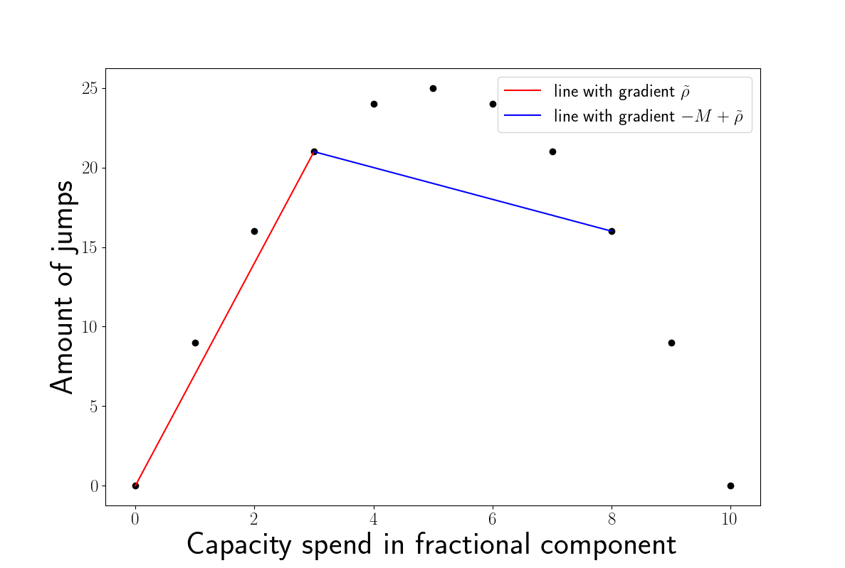
Figure 4: Visualization of the connection between the capacity used on the fractional component and the amount of jumps (cut edges) in the fully connected graph. For the example visualized above the values are given by $\Delta=8$, $\Delta_{r}=3$ and $|G|=10$. We can see that $\tilde{\rho}$ and $M$ are chosen such that the amount of jumps is always affinely underestimated.

For the optimal solution to the linear programming relaxation (LP) it holds that the right hand side of the equation is equal to $-M\Delta_{out}$ as all $\beta_{i,j}$ and $\gamma_{i,j}$ are equal to zero and the sum of the $\delta_{i,j}$ regarding the subset $H$ is exactly $\Delta_{out}$ by construction. The left side of the equation is however strictly larger than $M\Delta_{out}$ because $\tilde{\rho}>0$ and $\sum_{(i,j)\in G}\delta_{i,j}>0$. Thus this solution is cut off by the constructed inequality improving the relaxation formulation.

5.1.2 Cutting plane derived from a bounding box

In the previous subsection we have used the fully connected graph to obtain a valid cut. It admits the drawback that the computational time to calculate the weights grows quadratically in the size of the fractional component. In the worst case the fractional component is identical to the whole graph. Thus for very large connected components the trade off between the computational time of the cut and the run time reduction obtained from adding the cut might not be worth it. Instead we want to calculate a, potentially weaker, cut with a significantly lower computational demand.

The idea is that instead of only considering the jumps in the fractional component we find the smallest bounding box containing the component and add a cut using the minimum cut ratio on this rectangular subgraph. We use the same setting as in the previous subsection detailed in Assumption 1 and define $B\coloneqq\{(i,j)\in\Omega\ |\ \exists(i,k),(\ell,j)\in F\}$ as the smallest bounding box containing $F$ for which we assume that the previous control in the nodes is $0$ for now. Furthermore, we define $H_{B}\coloneqq H\setminus B$ and $\Delta_{B}=\Delta-\sum_{(i,j)\in H_{B}}\delta_{i,j}^{*}$ and $\Delta_{out_{B}}=\sum_{(i,j)\in H_{B}}\delta_{i,j}^{*}$.

We recall that for the bounding box we can underestimate the amount of cut edges for a given used capacity $K$ with the formula given in Lemma 1 which we already used for the NP-hardness conjectures. Note that in the original formulation our $B$ was called $G$.

Theorem 9.

Let $\Delta_{out_{B}}$ be an integer value between $0$ and $\Delta$. Let $B$ be a $\tilde{n}\times\tilde{m}$ rectangular subgraph of the grid with $x_{i,j}=0$ for all $(i,j)\in B$ and $H_{B}$ be a subgraph of the grid with $|H_{B}|=\Delta_{out_{B}}$. Let $B$ and $H_{B}$ be disjoint. Then every feasible point of (IP) fulfills the inequality

$$c_{\rho}\sum_{(i,j)\in B}\delta_{i,j}\leq\sum_{\begin{subarray}{c}((i,j),(i+1,j))\\ \in B\times B\end{subarray}}\beta_{i,j}+\sum_{\begin{subarray}{c}((i,j),(i,j+1))\\ \in B\times B\end{subarray}}\gamma_{i,j}+M(\Delta_{out_{B}}-\sum_{(i,j)\in H_{B}}\delta_{i,j}).$$

with $c_{\rho}\coloneqq\min_{0<K\leq\Delta-\Delta_{out_{B}}}\frac{\min\{\lfloor\sqrt{K}\rceil+\lceil\sqrt{K}\rceil,\tilde{n},\tilde{m},\lfloor\sqrt{\tilde{n}\tilde{m}-K}\rceil+\lceil\sqrt{\tilde{n}\tilde{m}-K}\rceil\}}{K}$ and $M\coloneqq c_{\rho}+2$.

Proof.

The Lemma 1 showed that $c_{\rho}$ is a lower bound for the amount of jumps in a $\tilde{n}\times\tilde{m}$ rectangular graph if at most $\Delta-\Delta_{out_{B}}$ nodes are set to $1$. Thus, it follows that the inequality holds if the $M$ is chosen sufficiently large. In the proof of Lemma 1 it was shown that the amount of jumps for $K$ nodes set to $1$ and $K+1$ nodes set to $1$ differs by at most $2$. It follows that the first term in the definition of $M$ negates the effect of the term on the left-hand side for values of $K$ larger than $\Delta-\Delta_{out_{B}}$ while the second term accounts for the highest possible decrease in the amount of jumps which is no more than $2$ for each additional node set to $1$. ∎

The relevant computational demands are determining the bounding box and the capacity used by the solution to (LP) in the nodes of the bounding box. These demands are linear in the size of the bounding box. In the worst case the size of the bounding box is quadratic in the size of the fractional component, but is bounded by the size of the grid which ensures that the calculation of the cut is significantly faster than the calculation of the previous cut for large fractional components.

Remark 4.

For the construction we have assumed that the previous controls in all nodes in the whole bounding box are $0$. This is however not needed and only done for the sake of clarity. If $c_{2}$ is the number of nodes with a previous control of $1$ the described cuts are valid if we instead use the formula $\min\{\lfloor\sqrt{K}\rceil+\lceil\sqrt{K}\rceil,\tilde{n},\tilde{m},\lfloor\sqrt{\tilde{n}\tilde{m}-K-c_{2}}\rceil+\lceil\sqrt{\tilde{n}\tilde{m}-K-c_{2}}\rceil\}$ to underestimate the amount of jumps and only consider $\delta_{i,j}$ on the left-hand side with $x_{i,j}=0$. This is a direct consequence of applying the original formula in Lemma 1 with $\tilde{K}=K+n_{c}$ for $n_{c}\in[0,c_{2}]\cap\mathbb{N}$.

5.2 Primal heuristics

We have already seen in Subsection 3.4 that substructures of the grid can correspond to one-dimensional problems of (TR-IP). We want to use this property to improve any feasible point found by the integer programming solver. Let $(\tilde{d},\tilde{\delta},\tilde{\beta},\tilde{\gamma})$ be a feasible point of $\eqref{eq:ip}$ with $N=M$. We assume $N$ to be even for sake of clarity but the arguments hold for odd $N$. We consider the problem

$$\begin{aligned} \min_{d,\delta,\beta,\gamma}\quad&\sum_{i=1}^{N}\sum_{j=1}^{M}c_{i,j}d_{i,j}+\alpha\left(\sum_{j=1}^{M}\sum_{i=1}^{N-1}\beta_{i,j}+\sum_{i=1}^{N}\sum_{j=1}^{M-1}\gamma_{i,j}\right)\\ \text{s.t.}\quad&(d,\delta,\beta,\gamma)\in P_{\Delta},\\ &d\in\mathbb{Z}^{N\times M}\text{ and }d_{i,j}=\tilde{d}_{i,j}\text{ for }i\in\{2,4,\ldots,N\},j\in\{1,\ldots,N\}.\end{aligned}$$ (red IP)

Like the one-dimensional problem, the problem (red IP) can be solved by a shortest-path approach with the same graph structure and a slight variation of the weights to consider the jumps to the fixed nodes, see Appendix C for more details. We now show that a solution of (red IP) will always have an objective value no worse than the point $(\tilde{d},\tilde{\delta},\tilde{\beta},\tilde{\gamma})$ used for the construction of the problem.

Theorem 10.

Let $(\tilde{d},\tilde{\delta},\tilde{\beta},\tilde{\gamma})$ be a feasible point of $\eqref{eq:ip}$ with $N=M$. Then every solution of the problem (red IP) is feasible for (IP) and has a lower or equal objective value compared to the objective value of $(\tilde{d},\tilde{\delta},\tilde{\beta},\tilde{\gamma})$ regarding the objective function of (IP).

Proof.

The problem (red IP) can be derived from (IP) by adding additional constraints. Thus the objective functions conincide and the feasible set of (red IP) is a subset of (IP). The point $(\tilde{d},\tilde{\delta},\tilde{\beta},\tilde{\gamma})$ is feasible for (red IP). Thus any solution of (red IP) has a objective value lower or equal to the objective value of $(\tilde{d},\tilde{\delta},\tilde{\beta},\tilde{\gamma})$ and is feasible for (IP). ∎

We can now use this improved feasible point to construct a new problem of the form (red IP) with different fixed $d$ entries and repeat this process. In our algorithm we alternately fix the entries $d_{i,j}$ with $i\in\{1,\ldots,N\},j\in\{1,3,\ldots,N-1\}$, then $d_{i,j}$ with $i\in\{1,\ldots,N\},j\in\{2,4,\ldots,N\}$, then $d_{i,j}$ with $i\in\{1,3,\ldots,N-1\},j\in\{1,\ldots,N\}$ and finally $d_{i,j}$ with $i\in\{2,4,\ldots,N\},j\in\{1,\ldots,N\}$. We continue this process until none of the $4$ variations produce an improved feasible point. This process terminates finitely as there are only finitely many feasible points for the original problem $\eqref{eq:trip}$ and in each finite loop we improve the objective value.

5.3 Branching rules

We propose a branching rule motivated by the primal heuristic. In the previous subsection we observed that fixing half of the nodes allows us to obtain a one-dimensional problem and use a shortest path approach to obtain an optimal solution. This shows us that fixing the nodes in an order which follows this strategy might be preferable in order to come closer to a problem class that is more efficiently solvable as seen in Subsection 5.2. Thus we choose to fix the nodes in even rows and even columns first as these nodes are the most significant for the case that the even rows or columns are fixed and we optimize over the remaining nodes.

6 Computational experiments

To assess the performance of the tools analyzed in Section 5 we introduce an advection-diffusion problem in Subsection 6.1 that serves as our benchmark problem. We run the SLIP algorithm proposed in [21] for a uniform square grid of size $N\times N$ and binary controls $\Xi=\{0,1\}$ to produce subproblems of the form (TR-IP) for $5$ different values for the parameter $\alpha$. We compare $8$ different combinations of the proposed tools for the time to reach optimality and the gap closed after a given time. Further details are given in Subsection 6.2. Moreover, we examine if the size of the fractional component in the root linear programming relaxation is an indicator for the hardness of the problem (TR-IP) and approximation quality of the Lagrangian relaxation.

6.1 Benchmark problem

Our advection-diffusion benchmark problem on $\Omega=(0,1)^{2}$ reads

$$\begin{aligned} \min_{u,w}&\frac{1}{2}||u-u_{d}||^{2}_{L^{2}(\Omega)}+\alpha\operatorname*{TV}(w)\\ \text{s.t. }&-\varepsilon\Delta u+c\cdot\nabla u=w\text{ in }\Omega,\ u|_{\Gamma_{1}}=0,\ u|_{\Gamma_{2}}(x,y)=\sin(2\pi(x-0.25)),\\ &w(x)\in\{0,1\}\end{aligned}$$ (AD)

with $\varepsilon=0.075$ and $c=(\cos(\pi/32),\sin(\pi/32)))^{T}$. For the boundary we define two subsets $\Gamma_{1}=([0,0.25)\cup(0.75,1])\times\{0\}\cup\{0,1\}\times(0,1)$ and $\Gamma_{2}=[0.25,0.75]\times\{0\}$ for Dirichlet boundary conditions. The remaining subset has a free boundary condition. We execute the SLIP algorithm on discretizations of the domain and PDE. We use the python package FEniCSx, see [28, 29, 3, 1], for the discretization of the domain, the PDE, and the gradient computation, where we follow a first-discretize, then-optimize principle.

6.2 Computational Setup

We run the SLIP algorithm with the values $N=M\in\{32,64\}$ and $\alpha\in\{4\times 10^{-4},4\sqrt{5}\times 10^{-4},2\times 10^{-3},2\sqrt{5}\times 10^{-3},1\times 10^{-2}\}$ as well as $N=M=96$ and $\alpha\in\{4\sqrt{5}\times 10^{-4},2\times 10^{-3},2\sqrt{5}\times 10^{-3}\}$, where we chose only three values due to the computational demand. We set $\Delta^{0}=\frac{1}{16}N^{2}$ and choose $\sigma=0.0001$ in Algorithm 1. To compare the approaches we solve each of the subproblems with the different combinations of tools that are detailed in Table 1. We model the integer programs without the variables $\delta$ because they are not needed for the binary case as we can just use $d$ as the absolute value and add signs in the remaining inequalties depending on the previous control value. We employ the integer programming solver Gurobi 10.0.0, see [16], and set a time limit of $1$ hour before returning the current best primal point in the subproblem solver to generate instances of the form (TR-IP). We keep the default optimality tolerances of Gurobi which means a solution is considered optimal if the gap is less than 0.001. We include the time to build the model in Gurobi in our measurements. Thus the results include the whole run times of the subproblems but not the whole SLIP algorithm. The tools are implemented in C++ and we use pybind11, see [19], to call the implemented functions from python. The cuts are added as lazy constraints to ensure that they are added to the model description. For a fair comparison the value PreCrush is set to $1$ even when no cuts are added because this setting significantly reduced the run time in our preliminary experiments. The laptop for the experiments has an Intel(R) Core i7(TM) CPU with eight cores clocked at 2.5 GHz and 64 GB RAM.

Table 1: Abbreviations for the different solution approaches (combinations of tools from Section 5).

tools (Section)	none	p	b	c	p-b	p-c	b-c	p-b-c
Primal (Section 5.2)	-	x	-	-	x	x	-	x
Branching Rule (Section 5.3)	-	-	x	-	x	-	x	x
Cuts (Section 5.1)	-	-	-	x	-	x	x	x

6.3 Comparison of the computational results for the different approaches

For the smallest value $N=32$ solving all $114$ subproblems, see Table 2, only takes around $2$ to $3$ minutes. The approaches b-c and p-b-c produce the best cumulative times with $115$ and $116$ seconds as seen in Table 3. On average it takes both approaches 1 second to solve an instance of this size. In general, the approaches using cuts (c, p-c, b-c, p-b-c) perform better compared to the alternatives which is also reflected in the median run times depicted in Table 4 where the approach c performs best. The approaches b-c and p-b-c perform best with a cumulative run time improvement of around 25 percent compared to the approach none.

Table 2: Number of instances produced by the SLIP algorithm for the different values for $N$ and $\alpha$.

$N$	$\alpha=4\times 10^{-4}$	$\alpha=4\sqrt{5}\times 10^{-4}$	$\alpha=2\times 10^{-3}$	$\alpha=2\sqrt{5}\times 10^{-3}$	$\alpha=1\times 10^{-2}$
$N=32$	40	34	24	15	1
$N=64$	70	38	53	19	1
$N=96$	-	74	173	35	-

Table 3: Cumulative run times of the different approaches for $N\in\{32,64,96\}$ and the $5$ values for $\alpha$. We note that all is the cumulative run time for all instances for the value of $N$.

N	$\alpha$	none	p	b	c	p-b	p-c	b-c	p-b-c
32	$4\times 10^{-4}$	19	20	20	22	21	22	22	22
	$4\sqrt{5}\times 10^{-4}$	23	23	23	22	24	23	23	23
	$2\times 10^{-3}$	35	36	36	27	37	27	27	27
	$2\sqrt{5}\times 10^{-3}$	48	47	40	33	39	31	30	30
	$1\times 10^{-2}$	30	31	23	17	23	17	14	14
	all	154	157	142	120	143	120	115	116
64	$4\times 10^{-4}$	2905	2932	2646	1492	2670	1470	971	955
	$4\sqrt{5}\times 10^{-4}$	1540	1537	1296	594	1289	606	645	706
	$2\times 10^{-3}$	7343	7437	5370	3625	5497	3531	2894	2876
	$2\sqrt{5}\times 10^{-3}$	16643	14554	8586	9326	8822	8874	6624	6448
	$1\times 10^{-2}$	3600	3601	3601	3602	3601	3601	3601	3601
	all	32032	30061	21498	18639	21878	18082	14736	14586
96	$4\sqrt{5}\times 10^{-4}$	61292	-	-	-	-	-	-	46382
	$2\times 10^{-3}$	383256	-	-	-	-	-	-	350115
	$2\sqrt{5}\times 10^{-3}$	78743	-	-	-	-	-	-	65587
	all	523292	-	-	-	-	-	-	462083

Table 4: Median run times of the different approaches for $N\in\{32,64,96\}$ and the $5$ values for $\alpha$. We note that all is the median run time for all instances for the value of $N$.

N $\alpha$ none p b c p-b p-c b-c p-b-c 32 $4\times 10^{-4}$ 0.31 0.32 0.33 0.43 0.34 0.50 0.44 0.47 $4\sqrt{5}\times 10^{-4}$ 0.68 0.63 0.66 0.61 0.61 0.64 0.67 0.69 $2\times 10^{-3}$ 1.28 1.24 1.29 1.00 1.32 1.00 0.89 0.90 $2\sqrt{5}\times 10^{-3}$ 2.71 2.64 2.35 1.67 2.33 1.66 1.57 1.62 $1\times 10^{-2}$ 29.71 30.72 22.55 16.83 22.59 16.80 13.79 13.76 all 0.74 0.77 0.78 0.67 0.83 0.69 0.71 0.72 64 $4\times 10^{-4}$ 12.47 13.38 12.11 11.32 12.18 11.42 10.89 11.00 $4\sqrt{5}\times 10^{-4}$ 10.98 11.43 10.26 9.23 10.35 8.66 8.95 8.44 $2\times 10^{-3}$ 82.84 83.35 61.40 37.48 63.12 37.40 29.83 29.66 $2\sqrt{5}\times 10^{-3}$ 153.04 152.87 137.63 83.62 137.80 83.58 86.41 86.38 $1\times 10^{-2}$ 3600.46 3600.57 3600.55 3602.37 3600.54 3601.04 3601.15 3601.15 all 26.78 26.88 23.00 16.95 23.77 16.33 15.02 14.40 96 $4\sqrt{5}\times 10^{-4}$ 298.61 - - - - - - 121.39 $2\times 10^{-3}$ 2617.74 - - - - - - 2433.26 $2\sqrt{5}\times 10^{-3}$ 3600.93 - - - - - - 1705.99 all 1579.09 - - - - - - 989.70

This behaviour extends to the case with $N=64$ with an improvement of $46$ percent. For this discretization most instances are solved within $600$ seconds for the different approaches. We note that the approaches using the cuts (c, p-c, b-c, p-b-c) perform better than those which do not. In general, the approaches which include the primal heuristic (p, p-b, p-c, p-b-c) only seem to improve the run time if combined with the cuts (p-c, p-b-c). Both observations are illustrated by the performance plots in Figure 5. The best approach for both $N=32$ and $N=64$ is the combination of all the tools as the cumulative run times are lowest or second lowest, see Table 3. For $N=64$ and $\alpha=1\times 10^{-2}$ the instance could not be solved by any time limit. All approaches produce the same primal point with objective value $0$. The objective lower bounds produced vary from $-0.18$ by none to $-0.08$ by p-b-c.

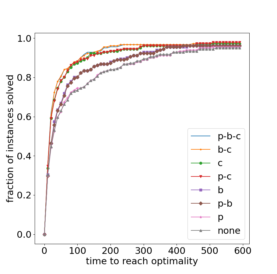
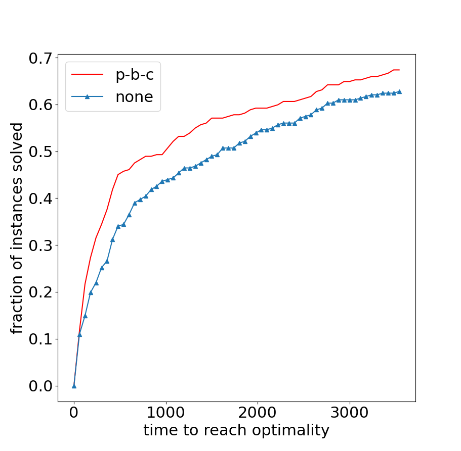
Figure 5: Performance plots for $N=64$ (left) and $N=96$ (right). The plots visualize what fraction of the instances are solved after a given time. For $N=64$ nearly all instances are solved after $600$ seconds while for $N=96$ a significant number of instances are not solved within the time limit of $1$ hour.

For $N=96$ we only compare the approaches with no tools and all tools combined. An improvement of $12$ percent for the cumulative run time is achieved by employing all proposed tools. We note that a larger improvement of $37$ percent is achieved regarding the median run times. This effect might be due to the significant number of instances reaching the time limit of $1$ hour which is visualized by the performance plot in Figure 5. There were $68$ instances which could not be solved within the time limit by either approach. Additionally $23$ instances could not be solved by p-b-c but could be solved by none, while the opposite case occurred for $37$ instances. The mean duality gap is reduced from $2.6$ percent to $2.3$ percent by p-b-c. Furthermore, the highest occurring duality gap is also reduced as visualized by the violin plot in Figure 6. The primal values were significantly better (exceeding the tolerance of the integer programming solver) for the approach ”none” in $15$ cases while p-b-c produced significantly better primal values in $23$ cases.

We reran the experiments with a time limit of $3$ hours for all instances only solved by either p-b-c or none to get a clearer picture. We see that now the new cumulative run times of the approaches are 530781 seconds for p-b-c and 655740 seconds for none. Thus p-b-c improves the run time by 19 percent compared to none. We note that 3 instances for p-b-c still reached the new time limit while 7 instances reached the new time limit for none.

In many cases the feasible point obtained from the Lagrangian relaxation did not produce an approximation as no capacity was used. However, for $N=32$ there were $21$ instances for which at least half of the capacity was used by the feasible point. This effect gets smaller as $N$ increases as for $N=64$ there were $16$ such instances while for $N=96$ only $5$ instances produced such a feasible point from the Lagrangian relaxation. In these cases the approximation guarantee from Theorem 2 was always achieved. In $5$ cases the feasible point was optimal and in the remaining cases the feasible point was strictly better than the approximation guarantee derived in Theorem 2.

In Figure 7 we see that a larger fractional component in the root linear program corresponds to a higher run time. We note that for $N=96$ the linear regression is negatively impacted by the large amount of instances reaching the time limit and other regressions may be a better fit for the data but still shows the general trend.

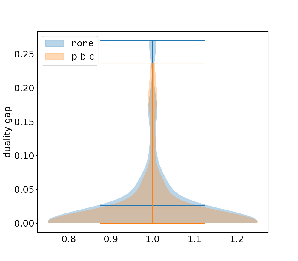
Figure 6: The violin plot shows the distribution of the remaining duality gap after the time limit of $1$ hour. The lines in the middle mark the mean duality gaps for all instances.

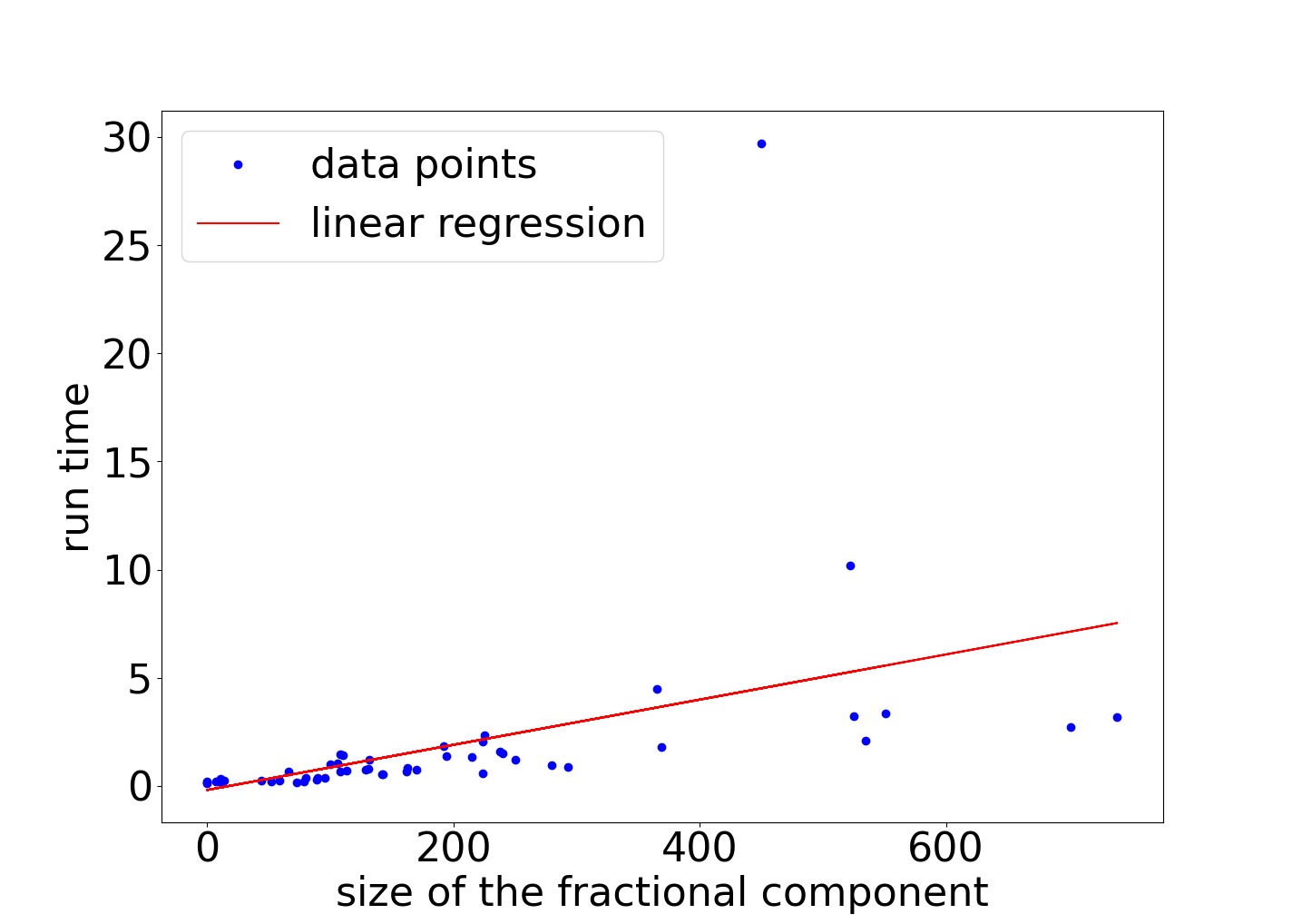
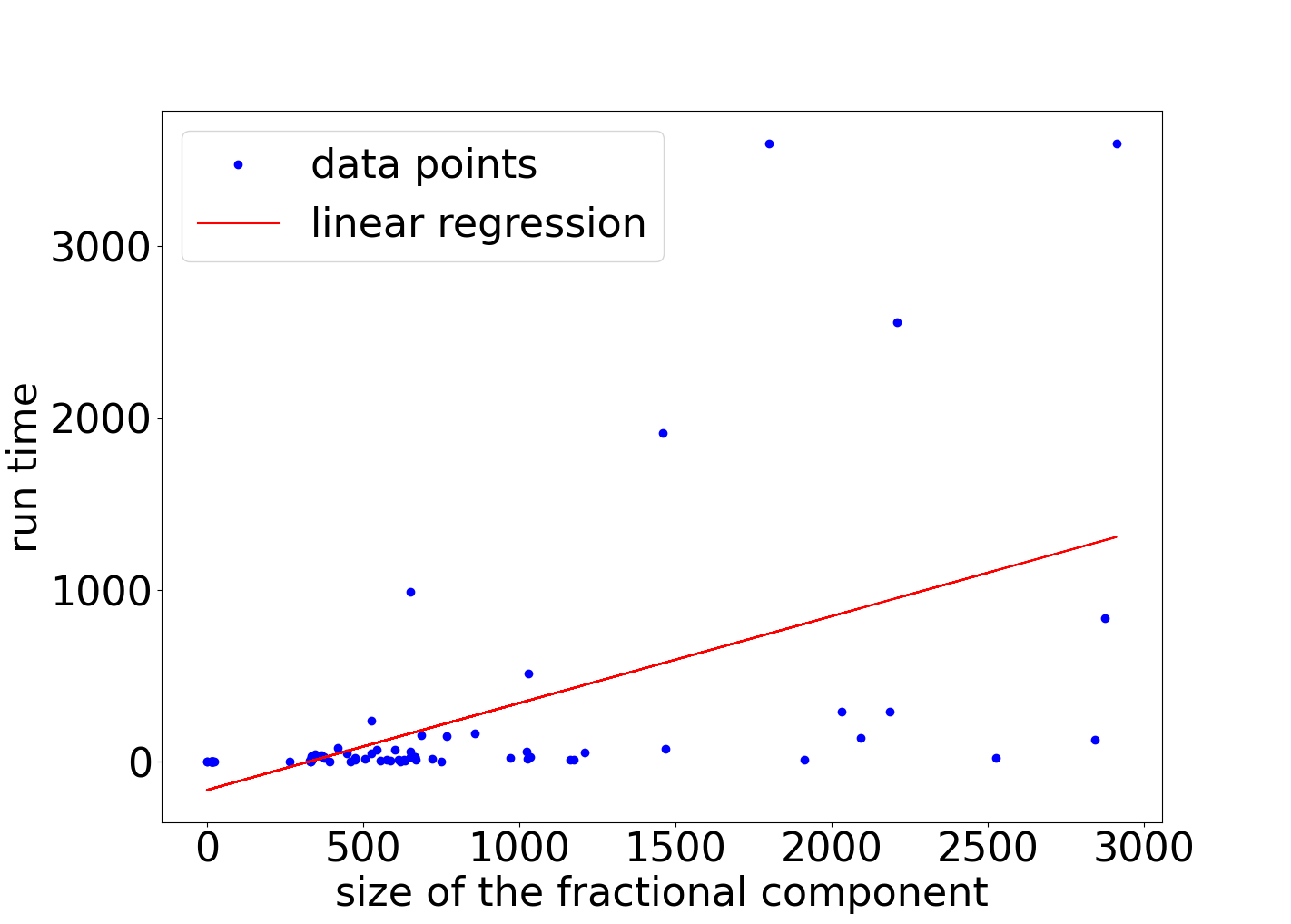
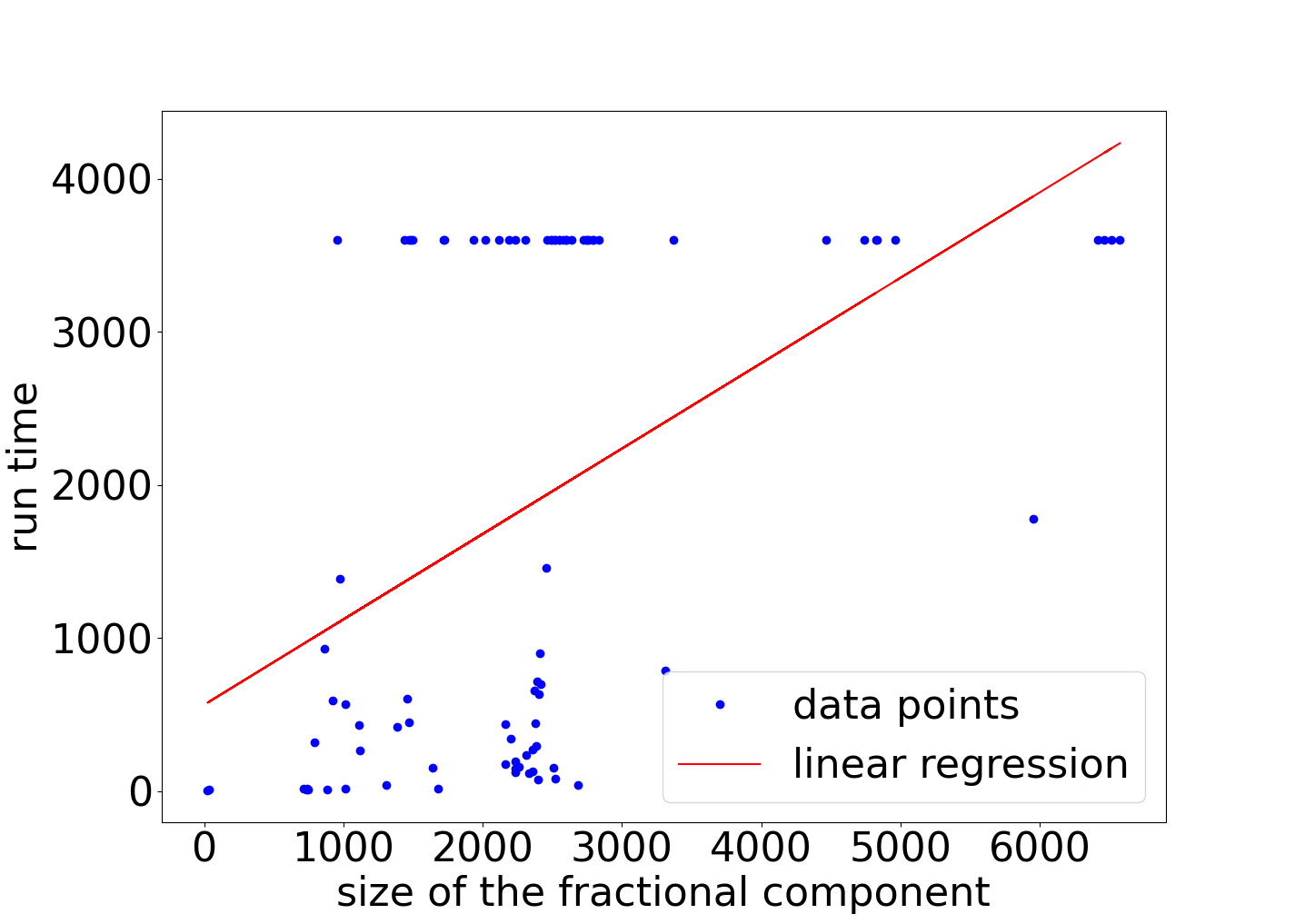
Figure 7: From left to right the plots show the relation between the size of the fractional component and the run time for $N=32$ and $\Delta=64$, $N=64$ and $\Delta=256$, $N=96$ and $\Delta=576$. In each plot the red line represents the linear regression of the data which itself is plotted as the blue points.

7 Conclusion

We have provided structural findings for the underlying polyhedron and its vertices as well as a conditional p-approximation. We have used these findings and developed tools to improve the run time of the integer programming solver. Our experimental results show that especially the proposed cutting planes reduce the run time substantially. Depending on the problem size the run time is reduced by up to $46$ percent. For larger values of $N$ this effect is reduced but improves if larger compute times are acceptable. We attribute this in parts to the fact that the inequalities describing the model only have a constant number of non-zero entries while the amount of non-zero entries in the added inequalities can grow with the size of the grid.

Our analysis and computational results motivate several avenues for future research.

The proposed cuts may be improved in two ways. First, for the cut using the bounding box from Section 5.1.2 we use the same coefficient for every node in the fractional component in the added inequality. However, the construction of the cutting plane implies that a minimum bisection which has to contain specific nodes on specific sides allows for sharper coefficients and thus an improvement of the cut. Second, we have observed that the bounding box can be significantly larger than the fractional component. In the worst case the size of the bounding box is quadratic in the size of the fractional component. Computing the actual minimum bisection of the fractional component instead of the bounding box would produce an inequality with fewer non-zero coefficients.

In addition, cuts based on the fractional component itself also seem attractive because the size of the fractional component in the root linear program can indicate the hardness of the instance as we have seen in Figure 7.

While the Lagrangian relaxation provides a p-approximation, the feasible points were only useful for few instances in a similar vein to a Cauchy point in a trust-region algorithm as in many cases the used capacity is too small and thus the approximation guarantee is not good enough.

In order to leverage the achieved significant speed-up for medium-sized instances, we believe that domain decomposition techniques on function space level are both attractive and viable so that one obtains such instances of (TR-IP) in practice.

Moreover, as we have noted in Section 2, the current discretization of the superordinate problem in function space currently implies an anisotropic discretization of the total variation. Ongoing research shows that this may be overcome by successively adding additional linear inequalities to (TR-IP). Their effect on the problem structure and solution process is important for further research and advancing the overall methodology but also significantly beyond the scope of this work.

Appendix A Proof of Lemma 1

In this section we prove the Lemma 1 which we restate here.

Lemma 3.

Let $G(V,A)$ be a $\tilde{n}\times\tilde{m}$ rectangular subgraph of the infinite grid $\mathbb{Z}\times\mathbb{Z}$. Then for a subset $U\subset G$ of size $K$ it holds that

$$|\partial U|\geq\min\{\lfloor\sqrt{K}\rceil+\lceil\sqrt{K}\rceil,\tilde{n},\tilde{m},\lfloor\sqrt{\tilde{n}\tilde{m}-K}\rceil+\lceil\sqrt{\tilde{n}\tilde{m}-K}\rceil\}$$

where $\partial U=\{(v,w)\in A\ |\ v\in U,\ w\in G\setminus U\}$ is the set of cut edges.

Proof.

We start with the infinite grid $\mathbb{Z}\times\mathbb{Z}$ before returning to the rectangular subgraph. We want to determine a subset $U$ of the infinite grid with size $K=|U|$ such that the number of edges between $U$ and its complement in the infinite grid is minimized.

It is straightforward to see that $U$ has to be a connected subset. Assume that $U$ contains two separate connected components. Then we could shift one component until it becomes adjacent to the other component and reduce the amount of edges between $U$ and its complement in the infinite grid by at least one edge. Thus $U$ has to be a connected subset.

Let $v_{\ell}=(x_{\ell},y_{\ell}),v_{r}=(x_{r},y_{r}),v_{b}=(x_{b},y_{b}),v_{t}=(x_{t},y_{t})$ be the leftmost, rightmost, bottommost, and topmost nodes in the set $U$. Then the complement in the infinite grid $U^{C}$ contains the node pairs $(x_{\ell}-1,y),(x_{r}+1,y)$ for $y\in[y_{b},y_{t}]$. If we connect these pairs of the form $(x_{\ell}-1,y),(x_{r}+1,y)$ by a straight line we pass through at least one node in $U$ and thus obtain at least two cut edges per pair. The same holds true for the pairs $(x,y_{b}-1),(x,y_{t}+1)$ for $x\in[x_{\ell},x_{r}]$. Thus there have to be at least $2(y_{t}-y_{b})+2(x_{r}-x_{\ell})$ cut edges between $U$ and $U^{C}$. For a set of size $K$ this implies that $2\lceil\sqrt{K}\rceil+2\lfloor\sqrt{K}\rceil$ is a lower bound for the amount of edges between $U$ and $U^{C}$ (meaning $U$ should be a structure as close to a square as possible).

We can transfer these insights to the case of the positive orthant, the infinite grid $\mathbb{N}\times\mathbb{N}$. The argumentation from before also holds for the $\mathbb{N}\times\mathbb{N}$ grid but we now assume that for the leftmost node $v_{\ell}$ it holds that $v_{\ell}=(0,y_{\ell})$ and for the bottommost node $v_{b}$ it holds that $v_{b}=(x_{b},0)$ which implies that the minimum is halved meaning the minimum number of edges between $U$ and its complement in the $\mathbb{N}\times\mathbb{N}$ grid is $y_{t}+x_{r}$ or $\lceil\sqrt{K}\rceil+\lfloor\sqrt{K}\rceil$.

We now consider the case of the rectangular subgraph $G$. If $K<\min\{\tilde{n},\tilde{m}\}$ the situation does not differ from the infinite grid $\mathbb{N}\times\mathbb{N}$. Due to the concavity of the square root it is ensured that $U$ is a connected component because in the case of two components the minimum amount of edges would be two times the sum of the square roots of the number of nodes in the components. It follows that we obtain the same optimal structures and lower bounds for which examples are shown in the first two grids in Figure 2. If $K$ is bigger than half the size of $G$ and $\tilde{n}\tilde{m}-K<\min\{\tilde{n},\tilde{m}\}$ we instead consider the complement and obtain $\lfloor\sqrt{\tilde{n}\tilde{m}-K}\rceil+\lceil\sqrt{\tilde{n}\tilde{m}-K}\rceil$ edges instead.

It remains the case that $K\geq\min\{\tilde{n},\tilde{m}\}$ and $\tilde{n}\tilde{m}-K\geq\min\{\tilde{n},\tilde{m}\}$ . Because it is possible that edges to the complement only arise in one of the four directions which gives rise to new optimal structures. If $K$ is an integer multiple of $\tilde{n}$ e.g. $K=c\tilde{n}$ then we can choose $U$ as the first $c$ rows to obtain a set $U$ of size $K$ with exactly $\tilde{n}$ edges to its complement in $G$ which is depicted in the third grid in Figure 2. The same argumentation holds if $K$ is an integer multiple of $\tilde{m}$. It is evident that this new structure is optimal iff $\tilde{n}<\lceil\sqrt{K}\rceil+\lfloor\sqrt{K}\rceil$ and $\tilde{n}<\lfloor\sqrt{\tilde{n}\tilde{m}-K}\rceil+\lceil\sqrt{\tilde{n}\tilde{m}-K}\rceil$. If $(c+1)\tilde{n}>K>c\tilde{n}$ then either one of the structures derived from the infinite grid $\mathbb{N}\times\mathbb{N}$ is optimal or we can choose $U$ as the first $c$ rows and the part of the next row such that the size matches which implies $\tilde{n}+1$ cut edges, see the fourth grid in Figure 2. Thus $\tilde{n}$ is also a lower bound in this case. Combining these cases we obtain the statement. ∎

Appendix B Dual decomposition relaxation

In this section we introduce another relaxation which did not prove useful in our preliminary experiments but which might prove useful with slight variations in the future. In (IP) the terms modeling the total variation are split into sums over the auxiliary variables $\beta\in\mathbb{N}^{(N-1)\times M}$ and $\gamma\in\mathbb{N}^{N\times(M-1)}$. The corresponding linear inequalities are coupled through $d$. To obtain a new relaxation we first rewrite (IP) such that we split each entry in $d$ into two copies $d^{c}$ and $d^{r}$ where $d^{c}$ is used for the inequalities containing $\beta$ and $d^{r}$ for the inequalities containing $\gamma$. This will allow us to solve the resulting problem in polynomial time. Furthermore, this will provide a lower bound which can be tighter than the lower bound obtained from the linear relaxation. For the underlying grid as illustrated in Figure 1 this means that $d^{r}$ takes into account only the rows while $d^{c}$ considers only the columns. To ensure equivalence to (IP) we add coupling linear equalities to enforce that both copies are equal. We obtain the integer linear program

$$\begin{aligned} \min_{d^{r},d^{c},\delta^{r},\delta^{c},\beta,\gamma}\quad&\frac{1}{2}\sum_{i=1}^{N}\sum_{j=1}^{M}c_{i,j}d_{i,j}^{r}+\frac{1}{2}\sum_{i=1}^{N}\sum_{j=1}^{M}c_{i,j}d_{i,j}^{c}+\alpha\left(\sum_{j=1}^{M}\sum_{i=1}^{N-1}\beta_{i,j}+\sum_{i=1}^{N}\sum_{j=1}^{M-1}\gamma_{i,j}\right)\\ \text{s.t.}\quad&(d^{r},\delta^{r},\gamma)\in P_{r}\text{ and }(d^{c},\delta^{c},\beta)\in P_{c},\\ &d^{c}=d^{r}\text{ and }d^{r},d^{c}\in\mathbb{Z}^{N\times M}.\end{aligned}$$ (IP-DD)

where $P_{r}$ is the polyhedron defined by

$$(d^{r},\delta^{r},\gamma)\in P_{r} \Leftrightarrow/\begin{cases}\min\Xi\leq x_{i,j}+d^{r}_{i,j}\leq\max\Xi&\text{ for all }i\in[N],j\in[M],\\ -\gamma_{i,j}\leq x_{i,j+1}+d^{r}_{i,j+1}-x_{i,j}-d^{r}_{i,j}\leq\gamma_{i,j}&\text{ for all }i\in[N],j\in[M-1],\\ -\delta^{r}_{i,j}\leq d^{r}_{i,j}\leq\delta^{r}_{i,j}&\text{ for all }i\in[N],j\in[M],\\ \sum_{i=1}^{N}\sum_{j=1}^{M}\delta^{r}_{i,j}\leq\Delta,\end{cases}$$

and $P_{c}$ is the polyhedron defined by

$$(d^{c},\delta^{c},\beta)\in P_{c} \Leftrightarrow/\begin{cases}\min\Xi\leq x_{i,j}+d^{c}_{i,j}\leq\max\Xi&\text{ for all }i\in[N],j\in[M],\\ -\beta_{i,j}\leq x_{i+1,j}+d^{c}_{i+1,j}-x_{i,j}-d^{c}_{i,j}\leq\beta_{i,j}&\text{ for all }i\in[N-1],j\in[M],\\ -\delta^{c}_{i,j}\leq d^{c}_{i,j}\leq\delta^{c}_{i,j}&\text{ for all }i\in[N],j\in[M],\\ \sum_{i=1}^{N}\sum_{j=1}^{M}\delta^{c}_{i,j}\leq\Delta.\end{cases}$$

We briefly state that the constructed problem (IP-DD) is equivalent to (IP).

Lemma 4.

Let $(d,\delta,\beta,\gamma)$ be feasible for (IP). Then $(d^{r},d^{c},\delta^{r},\delta^{c},\beta,\gamma)$ with $d^{r}=d^{c}=d$, $\delta^{r}=\delta^{c}=\delta$ is feasible for (IP-DD) with the same objective value. If $(d^{r},d^{c},\delta^{r},\delta^{c},\beta,\gamma)$ is feasible for (IP-DD) then $(d,\delta,\beta,\gamma)$ with $d=d^{r}$ and $\delta=\delta^{r}$ is feasible for (IP) with the same objective value.

Proof.

Let $(d,\delta,\beta,\gamma)$ be feasible for (IP). We show that $(d^{r},d^{c},\delta^{r},\delta^{c},\beta,\gamma)$ with $d^{r}=d^{c}=d$ and $\delta^{r}=\delta^{c}=\delta$ is feasible for (IP-DD). We first note that $(d^{r},\delta^{r},\gamma)\in P_{r}$, which follows from $d=d^{r}$, $\delta=\delta^{r}$, and $(d,\delta,\beta,\gamma)\in P_{\Delta}$. By the same argumentation $(d^{c},\delta^{c},\beta)\in P_{c}$. The remaining constraints are obviously fulfilled. The objective values coincide because $d^{r}=d^{c}=d$ so that

$$\frac{1}{2}\sum_{i=1}^{N}\sum_{j=1}^{M}c_{i,j}d_{i,j}^{r}+\frac{1}{2}\sum_{i=1}^{N}\sum_{j=1}^{M}c_{i,j}d_{i,j}^{c}=\sum_{i=1}^{N}\sum_{j=1}^{M}c_{i,j}d_{i,j}$$

and the remaining terms are the same. The other implication can be proven in the same way by just switching the roles of $d^{r}$ and $d$ as well as of $\delta^{r}$ and $\delta$ and using $d^{r}=d^{c}$. ∎

Corollary 4.

Let $(d,\delta,\beta,\gamma)$ be a feasible point of (LP). Then $(d^{r},d^{c},\delta^{r},\delta^{c},\beta,\gamma)$ with $d^{r}=d^{c}=d$ and $\delta^{r}=\delta^{c}=\delta$ is feasible for the linear programming relaxation of (IP-DD) with the same objective value. On the other hand if $(d^{r},d^{c},\delta^{r},\delta^{c},\beta,\gamma)$ is feasible for the linear programming relaxation of (IP-DD) then $(d,\delta,\beta,\gamma)$ with $d=d^{r}$ and $\delta=\delta^{r}$ is feasible for (LP) with the same objective value.

Proof.

The argumentation from the previous proof holds as we just need to drop the integrality conditions from both problems. ∎

Remark 5.

The previous lemma and corollary also hold for $d=d^{c}$ and $\delta=\delta^{c}$ by symmetry of the problem.

We can now obtain a Lagrangian relaxation by moving the coupling constraint $d^{r}=d^{c}$ into the objective with a multiplier variable. The problem reads

$$\begin{aligned} \min_{d^{r},d^{c},\delta^{r},\delta^{c},\beta,\gamma}\quad&\frac{1}{2}\sum_{i=1}^{N}\sum_{j=1}^{M}c_{i,j}d_{i,j}^{r}+\frac{1}{2}\sum_{i=1}^{N}\sum_{j=1}^{M}c_{i,j}d_{i,j}^{c}+\alpha\left(\sum_{j=1}^{M}\sum_{i=1}^{N-1}\beta_{i,j}+\sum_{i=1}^{N}\sum_{j=1}^{M-1}\gamma_{i,j}\right)\\ &+\sum_{i=1}^{N}\sum_{j=1}^{M}\lambda_{i,j}(d^{r}_{i,j}-d^{c}_{i,j})\\ \text{s.t.}\quad&(d^{r},\delta^{r},\gamma)\in P_{r}\text{ and }(d^{c},\delta^{c},\beta)\in P_{c},\\ &d^{r},d^{c}\in\mathbb{Z}^{N\times M}\end{aligned}$$ (LR-DD)

and provides a lower bound on the objective of (IP-DD) for every $\lambda\in\mathbb{R}^{N\times M}$.

Theorem 11.

Let $\lambda\in\mathbb{R}^{N\times M}$ be fixed. Then the optimal objective value of (LR-DD) provides a lower bound for the optimal objective value of (IP-DD).

Proof.

Let $(d^{r},d^{c},\delta^{r},\delta^{c},\beta,\gamma)$ with $d^{r}=d^{c}$ be an arbitrary, feasible point of (IP-DD). Then this point is also feasible for (LR-DD). Because $d^{r}=d^{c}$ the equality $\sum_{i=1}^{N}\sum_{j=1}^{M}\lambda_{i,j}(d^{r}_{i,j}-d^{c}_{i,j})=0$ holds and the objective function values of (IP-DD) and (LR-DD) coincide. Thus the optimal objective value of (LR-DD) can not be higher than the optimal objective value of (IP-DD). ∎

The problem (LR-DD) can be decoupled into the linear programs

$$\begin{aligned} \min_{d^{r},\delta^{r},\gamma}\quad&\frac{1}{2}\sum_{i=1}^{N}\sum_{j=1}^{M}(c_{i,j}+2\lambda_{i,j})d_{i,j}^{r}+\alpha\sum_{i=1}^{N}\sum_{j=1}^{M-1}\gamma_{i,j}\\ \text{s.t.}\quad&(d^{r},\delta^{r},\gamma)\in P_{r}\text{ and }d^{r}\in\mathbb{Z}^{N\times M},\end{aligned}$$ (R-DD)

and

$$\begin{aligned} \min_{d^{c},\delta^{c},\beta}\quad&\frac{1}{2}\sum_{i=1}^{N}\sum_{j=1}^{M}(c_{i,j}-2\lambda_{i,j})d_{i,j}^{c}+\alpha\sum_{i=1}^{N-1}\sum_{j=1}^{M}\beta_{i,j}\\ \text{s.t.}\quad&(d^{c},\delta^{c},\beta)\in P_{c}\text{ and }d^{c}\in\mathbb{Z}^{N\times M},\end{aligned}$$ (C-DD)

which can be solved independently for $d^{r},\delta^{r},\gamma$ and $d^{c},\delta^{c},\beta$ in order to solve (LR-DD). Each of the resulting problems can be interpreted as a one-dimensional version of (TR-IP). We have already shown that the sum of the optimal values provides a lower bound. We are now interested in which cases this already allows for the construction of an optimal point for (IP-DD) and hence (IP).

Theorem 12.

Let $(d^{r,*},\delta^{r,*},\gamma^{*})$ be an optimal point for the problem (R-DD) and $(d^{c,*},\delta^{c,*},\beta^{*})$ be an optimal point for (C-DD). If $d^{r,*}=d^{c,*}$ holds, then $(d^{*},\delta^{*},\beta^{*},\gamma^{*})$ with $d^{*}=d^{r,*}$ and $\delta^{*}=\delta^{r,*}$ is optimal for (IP-DD) and hence (IP).

Proof.

The feasibility of the constructed point follows by construction because $d^{r,*}$ and $d^{c,*}$ adhere to the capacity constraint and the controls can only take control values in $\Xi$. Thus it remains to show the optimality.

Let $(d,\delta,\beta,\gamma)$ be feasible for (IP). Let $(d^{r,*},\delta^{r,*},\gamma^{*})$ be an optimal point for (R-DD) and $(d^{c,*},\delta^{c,*},\beta^{*})$ be an optimal point for (C-DD). Then the two inequalities

$$\sum_{i=1}^{N}\sum_{j=1}^{M}(\frac{1}{2}c_{i,j}-\lambda_{i,j})d_{i,j}+\alpha\sum_{i=1}^{N}\sum_{j=1}^{M-1}\gamma_{i,j}\geq\sum_{i=1}^{N}\sum_{j=1}^{M}(\frac{1}{2}c_{i,j}-\lambda_{i,j})d_{i,j}^{r,*}+\alpha\sum_{i=1}^{N}\sum_{j=1}^{M-1}\gamma_{i,j}^{*}$$

and

$$\sum_{i=1}^{N}\sum_{j=1}^{M}(\frac{1}{2}c_{i,j}+\lambda_{i,j})d_{i,j}+\alpha\sum_{i=1}^{N-1}\sum_{j=1}^{M}\beta_{i,j}\geq\sum_{i=1}^{N}\sum_{j=1}^{M}(\frac{1}{2}c_{i,j}+\lambda_{i,j})d_{i,j}^{c,*}+\alpha\sum_{i=1}^{N-1}\sum_{j=1}^{M}\beta_{i,j}^{*}$$

hold. The statement follows from adding both inequalities. ∎

Remark 6.

The split into one row and one column problem is the most straightforward split but other splits of $\beta$ and $\gamma$ into two sets are also possible although these might create subproblems which are not known to be pseudo-polynomially solvable.

The bound provided by a Lagrangian relaxation with an optimal Lagrange multiplier is at least as good as the bound provided by the linear programming relaxation, see [13]. Thus, it follows from Corollary 4 that the bound from (LR-DD) for an optimal $\lambda$, which maximizes the objective of (LR-DD), is at least as good as the bound from (LP). We provide a minimal example to show that the dual decomposition relaxation can also be superior to the linear relaxation by providing a tighter bound.

Example 2.

Let $N=M=2$, $\Delta=1$, $\alpha=1$,

$$c=\begin{pmatrix}-0.5&-0.5\\ -0.5&-0.5\end{pmatrix},\ x=\begin{pmatrix}0&0\\ 0&0\end{pmatrix}.$$

Then the unique optimal point of (R-DD) for $\lambda\equiv 0$ is $d^{r}\equiv 0$ and of (C-DD) for $\lambda\equiv 0$ is $d^{c}\equiv 0$. Thus $d\equiv 0$ is optimal for (IP) but the linear programming relaxation solution is

$$d=\begin{pmatrix}0.25&0.25\\ 0.25&0.25\end{pmatrix}$$

which shows that the dual decomposition relaxation is tighter in this case.

We believe that the relaxation did not produce better bounds in preliminary experiments because the capacity was significantly larger than each row or column. Thus it is possible to model the fractional component by setting the corresponding entries in some rows/columns to $1$ and the entries in the remaining rows/columns to $0$. The example above is chosen in such a way that this can not occur. We hypothesise that a different split which does not have this weakness may produce better bounds at the cost of an significantly increased computational demand.

Appendix C Graph construction for the primal improvement algorithm

In this subsection we show how the problems arising in the primal improvement approach can be solved as a shortest path problem. Let $(\tilde{d},\tilde{\beta},\tilde{\gamma},\tilde{\delta})$ be a feasible point of $\eqref{eq:ip}$ with $N=M$. We assume $N$ to be even for sake of clarity but the arguments also hold for odd $N$. We now consider the problem

$$\begin{aligned} \min_{d,\delta,\beta,\gamma}\quad&\sum_{i=1}^{N}\sum_{j=1}^{N}c_{i,j}d_{i,j}+\alpha\left(\sum_{j=1}^{N}\sum_{i=1}^{N-1}\beta_{i,j}+\sum_{i=1}^{N}\sum_{j=1}^{N-1}\gamma_{i,j}\right)\\ \text{s.t.}\quad&(d,\delta,\beta,\gamma)\in P_{\Delta},\\ &d\in\mathbb{Z}^{N\times N}\text{ and }d_{i,j}=\tilde{d}_{i,j}\text{ for }i\in\{2,4,\ldots,N\},j\in\{1,\ldots,N\}.\end{aligned}$$ (red IP)

The graph construction is similar to the one in [30] as we determine the control values of the nodes starting in the first row and continuing through the rows not already fixed but with two changes. The first change is that we need to consider the jumps to already fixed nodes given by $\tilde{d}_{i,j}$ which we do by adjusting the weights of the edges. The second change is that we need to adjust the weights as we start fixing a new row to model that we do not consider jumps from the last node of the previous row to the first node of the current row.

We construct a graph $G(V,A)$ with $\frac{N^{2}}{2}\Xi\Delta+2$ nodes including the source and the sink. There are $\frac{N^{2}}{2}$ layers with respectively $\Xi\Delta$ nodes where the nodes of the first layer are connected to the source and the nodes of the last layer are connected to the sink. Each node is only connected to nodes in the previous and following layer. We describe a node $v\in V$, excluding the source and the sink, as in the previous subsection as a triplet $v=(j,\delta,\eta)\in[\frac{N^{2}}{2}]\times\{x-y|x,y\in\Xi^{N}\}\times\{0,\ldots,\Delta\}.$ We define the notation $\ell(v)=j$, $p(v)=\delta$ and $\tilde{r}(v)=\eta.$

An edge $e$ exist between two nodes $u,v\in V\setminus\{s,t\}$ is defined by

$$e=(u,v)\in A\quad:\Longleftrightarrow\quad\left\{\begin{aligned} \ell(v)=\ell(u)+1,&\\ \text{there exists }(a,b)\in A\text{ with }b=u,&\\ \tilde{r}(v)=\tilde{r}(u)-\gamma_{\ell(v)}|p(v)|.&\\ \end{aligned}\right.$$

The first condition enforces the layer structure, while the second and last conditions ensure that the capacity constraint holds inductively. For a clearer presentation, we introduce $i(v)=a$ and $j(v)=b$ where $\ell(v)=(2a-1)N+b$. The weight of an edge $e=(u,v)\in A$ with $u,v\in V\setminus\{s,t\}$ is given by

$$w_{(u,v)}= c_{i(v),j(v)}+\begin{cases}|x_{i(v),j(v)}+p(v)-x_{i(u),j(u)}-p(u)|\quad&\text{if }i(u)=i(v),\\ 0\quad&\text{otherwise,}\end{cases}$$

$$+\begin{cases}|x_{i(v),j(v)}+p(v)-x_{i(v)+N,j(v)}-\tilde{d}_{i(v)+N,j(v)}|\quad&\text{if }i(v)<N,\\ 0\quad&\text{otherwise,}\end{cases}$$

$$+\begin{cases}|x_{i(v),j(v)}+p(v)-x_{i(v)-N,j(v)}-\tilde{d}_{i(v)-N,j(v)}|\quad&\text{if }i(v)>1,\\ 0\quad&\text{otherwise.}\end{cases}$$

We note that the second case distinction is not needed because $N$ was assumed to be even thus the first case is always fulfilled but the distinction is done anyway for sake of completeness for the case of an odd $N$. The source $s=(0,\emptyset,\Delta)$ is connected to all $v\in V$ in the first layer with sufficient remaining capacity, that is

$$(s,v)\in A\quad:\Longleftrightarrow\quad\ell(v)=1\text{ and }\tilde{r}(v)=\Delta-|p(v)|\gamma_{1}.$$

The weight is given by $w_{(s,v)}=c_{1}p_{N}(v)+|x_{2,1}+\tilde{d}_{2,1}-x_{1,1}-p(v)|$. The sink $t=(NM+1,\emptyset,0)$ is connected to each node $v\in V$ in the last layer that has an incoming edge, that is

$$(v,t)\in A\quad:\Longleftrightarrow\quad\text{there exists }u\in V\text{ such that }(u,v)\in A.$$

The weights have the value zero, that is $w_{(v,t)}=0$. Just like in [30] we can obtain an optimal solution for (red IP) by solving the shortest path problem from $s$ to $t$.

Figure 8: The nodes marked as $F$ are the fixed nodes in the grid. Each edge ending in at least one node not fixed beforehand represents one of the case distinction in the weights definition for the shortest path approach. A stands for the first, B for the second and C for the last case distinction in the definition of the weights.

References

- [1] M. S. Alnaes, A. Logg, K. B. Ølgaard, M. E. Rognes, and G. N. Wells. Unified form language: A domain-specific language for weak formulations of partial differential equations. ACM Transactions on Mathematical Software, 40, 2014.
- [2] A. Armon and U. Zwick. Multicriteria global minimum cuts. Algorithmica, 46:15–26, 2006.
- [3] I. A. Baratta, J. P. Dean, J. S. Dokken, M. Habera, J. S. Hale, C. N. Richardson, M. E. Rognes, M. W. Scroggs, N. Sime, and G. N. Wells. DOLFINx: the next generation FEniCS problem solving environment. preprint, 2023.
- [4] F. Bestehorn, C. Hansknecht, and C. Kirches. Mixed-integer optimal control problems with switching costs: a shortest path approach. Mathematical Programming, 188:621–652, 2021.
- [5] Y. Boykov and V. Kolmogorov. An experimental comparison of min-cut/max-flow algorithms for energy minimization in vision. IEEE Transactions on Pattern Analysis and Machine Intelligence, 26, 09 2004.
- [6] C. Buchheim, A. Grütering, and C. Meyer. Parabolic optimal control problems with combinatorial switching constraints – part iii: branch-and-bound algorithm. arXiv preprint arXiv:2401.10018, 2024.
- [7] A. Bürger, C. Zeile, A. Altmann-Dieses, S. Sager, and M. Diehl. An algorithm for mixed-integer optimal control of solar thermal climate systems with mpc-capable runtime. In 2018 European Control Conference (ECC), pages 1379–1385, 2018.
- [8] M. Burger, Y. Dong, and M. Hintermüller. Exact relaxation for classes of minimization problems with binary constraints. arXiv preprint arXiv:1210.7507, 2012.
- [9] G. Cristinelli, J. A. Iglesias, and D. Walter. Conditional gradients for total variation regularization with pde constraints: a graph cuts approach. arXiv preprint arXiv:2310.19777, 2023.
- [10] C. De Simone, M. Diehl, M. Jünger, P. Mutzel, G. Reinelt, and G. Rinaldi. Exact ground states of ising spin glasses: New experimental results with a branch-and-cut algorithm. Journal of Statistical Physics, 80:487–496, 1995.
- [11] J. Díaz and G. B. Mertzios. Minimum bisection is NP-hard on unit disk graphs. Information and Computation, 256:83–92, 2017.
- [12] A. E. Feldmann and P. Widmayer. An time algorithm to compute the bisection width of solid grid graphs. In Algorithms – ESA 2011, pages 143–154. Springer Berlin Heidelberg, 2011.
- [13] A. M. Geoffrion. Lagrangean relaxation for integer programming. In Mathematical Programming Study 2, pages 82–114. Springer, 1974.
- [14] M. Gerdts. Solving mixed-integer optimal control problems by branch & bound: a case study from automobile test-driving with gear shift. Optimal Control Applications and Methods, 26:1–18, 2005.
- [15] D. M. Greig, B. T. Porteous, and A. H. Seheult. Exact maximum a posteriori estimation for binary images. Journal of the Royal Statistical Society Series B: Statistical Methodology, 51(2):271–279, 1989.
- [16] Gurobi Optimization, LLC. Gurobi Optimizer Reference Manual, 2023.
- [17] M. Hahn, C. Kirches, P. Manns, S. Sager, and C. Zeile. Decomposition and approximation for pde-constrained mixed-integer optimal control. In Non-Smooth and Complementarity-Based Distributed Parameter Systems: Simulation and Hierarchical Optimization, pages 283–305. Springer, 2021.
- [18] F. M. Hante, G. Leugering, A. Martin, L. Schewe, and M. Schmidt. Challenges in optimal control problems for gas and fluid flow in networks of pipes and canals: From modeling to industrial applications. In Industrial Mathematics and Complex Systems, pages 77–122. Springer, 2017.
- [19] W. Jakob, J. Rhinelander, and D. Moldovan. pybind11 – seamless operability between c++11 and python, 2017. https://github.com/pybind/pybind11.
- [20] B. Korte and J. Vygen. Combinatorial Optimization. Springer, 6 edition, 2018.
- [21] S. Leyffer and P. Manns. Sequential linear integer programming for integer optimal control with total variation regularization. ESAIM: Control, Optimisation and Calculus of Variations, 28:66, 2022.
- [22] P. Manns and A. Schiemann. On integer optimal control with total variation regularization on multidimensional domains. SIAM Journal on Control and Optimization, 61(6):3415–3441, 2023.
- [23] J. Marko and G. Wachsmuth. Integer optimal control problems with total variation regularization: Optimality conditions and fast solution of subproblems. ESAIM: Control, Optimisation and Calculus of Variations, 29:81, 2023.
- [24] C. Nieuwenhuis, E. Töppe, and D. Cremers. A survey and comparison of discrete and continuous multilabel approaches for the Potts model. International Journal of Computer Vision (IJCV), 104:223–240, 2013.
- [25] C. H. Papadimitriou and M. Sideri. The bisection width of grid graphs. Mathematical Systems Theory, 29:97–110, 1990.
- [26] C. H. Papadimitriou and M. Yannakakis. On the approximability of trade-offs and optimal access of web sources. In Proceedings 41st Annual Symposium on Foundations of Computer Science, pages 86–92. IEEE, 2000.
- [27] S. Sager, M. Jung, and C. Kirches. Combinatorial integral approximation. Mathematical Methods of Operations Research, 73(3):363–380, 2011.
- [28] M. W. Scroggs, I. A. Baratta, C. N. Richardson, and G. N. Wells. Basix: a runtime finite element basis evaluation library. Journal of Open Source Software, 7(73):3982, 2022.
- [29] M. W. Scroggs, J. S. Dokken, C. N. Richardson, and G. N. Wells. Construction of arbitrary order finite element degree-of-freedom maps on polygonal and polyhedral cell meshes. ACM Transactions on Mathematical Software, 48(2):18:1–18:23, 2022.
- [30] M. Severitt and P. Manns. Efficient solution of discrete subproblems arising in integer optimal control with total variation regularization. INFORMS Journal on Computing, 35(4):869–885, 2023.
- [31] M. Soler, M. Kamgarpour, J. Lloret, and J. Lygeros. A hybrid optimal control approach to fuel-efficient aircraft conflict avoidance. IEEE Transactions on Intelligent Transportation Systems, 17(7):1826–1838, 2016.
- [32] O. Veksler. Efficient Graph-Based Energy Minimization Methods in Computer Vision. PhD thesis, Cornell University, USA, 1999.