Upper Bound of Bayesian Generalization Error in Partial Concept Bottleneck Model (CBM):
Partial CBM outperforms naive CBM
Abstract
Concept Bottleneck Model (CBM) is a methods for explaining neural networks. In CBM, concepts which correspond to reasons of outputs are inserted in the last intermediate layer as observed values. It is expected that we can interpret the relationship between the output and concept similar to linear regression. However, this interpretation requires observing all concepts and decreases the generalization performance of neural networks. Partial CBM (PCBM), which uses partially observed concepts, has been devised to resolve these difficulties. Although some numerical experiments suggest that the generalization performance of PCBMs is almost as high as that of the original neural networks, the theoretical behavior of its generalization error has not been yet clarified since PCBM is singular statistical model. In this paper, we reveal the Bayesian generalization error in PCBM with a three-layered and linear architecture. The result indcates that the structure of partially observed concepts decreases the Bayesian generalization error compared with that of CBM (full-observed concepts).
1 Introduction
Methods of artificial intelligence such as neural networks has been widely applied in many research and practical areas (Goodfellow et al., 2016; Dong et al., 2021), increasing the demand for the interpretability of the model to deploy more intelligence systems to the real world. The accountability of such systems needs to be verified in fields related directly to human life, such as automobiles (self-driving systems (Xu et al., 2020)) and medicine (medical image analysis (Koh et al., 2020; Klimiene et al., 2022)). In these fields, the models cannot be black boxes, and therefore, various interpretable machine learning procedures have been investigated (Molnar, 2020). The concept bottleneck model (CBM) reported by Kumar et al. (2009); Lampert et al. (2009); Koh et al. (2020) is one of the architectures used to make the model interpretable. The CBM has a novel structure, called a concept bottleneck structure, wherein concepts are inserted between the output and last intermediate layers. In this structure, the last connection from the concepts to the output is linear and fully connected; thus, we can interpret the weights of that connection as the effect of the specified concept to the output, which is similar to the coefficients of linear regression. Concept-based interpretation is used in knowledge discovery for chess (McGrath et al., 2022), video representation (Qian et al., 2022), medical imaging (Hu et al., 2022), clinical risk prediction (Raghu et al., 2021), computer-aided diagnosis (Klimiene et al., 2022), and other healthcare domain problems (Chen et al., 2021). For this interpretation, concepts must be labeled accurately as explanations of inputs to predict outputs. For example, the concepts need to be set as clinical findings that are corrected by radiologists to predict the knee arthritis grades of patients based on X-ray images of their knee (Koh et al., 2020). In other words, CBM cannot be trained effectively without an accurate annotation from radiologists. Thus, the labeling cost is higher than that of the conventional supervised learning machine. Further, the concept bottleneck structure limits the parameter region of the network and it decreases the generalization performance decreases (Hayashi & Sawada, 2023).
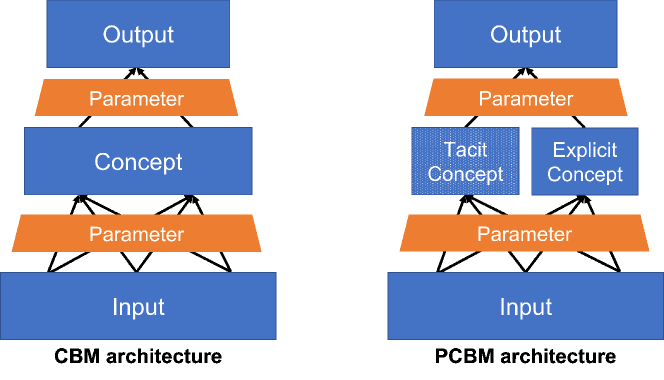
Sawada & Nakamura (2022) proposed CBM with an additional unsupervised concept (CBM-AUC) to decrease the annotation cost of concepts. The core idea of CBM-AUC is that concepts are partially replaced as unsupervised values, and they are classified into tacit and explicit knowledge. The former concepts are provided as observations similar to that in the original CBM, i.e., they are supervised. The latter ones are not observable and obtained as output from the previous connection, i.e., they are unsupervised. In the following, concepts corresponding to explicit/tacit knowledge are referred to as explicit/tacit concepts for simplicity. Futher, CBM-AUC uses a structure based on self-explaining neural networks (SENN) (Alvarez Melis & Jaakkola, 2018) for interpreting learned tacit concepts. In addition, partial CBM (PCBM) was developed in Li et al. (2022) and it only uses the above-mentioned core idea. For example, when the architecture is three-layered and linear (i.e., reduced rank regression), a neural network is trained, where , , and represent the input, output, and weight matrices, respectively. For CBM, there is an explicit concept vector , and the weight parameters are learned as and . The architectures of CBM and PCBM are illustrated in Figure 1. The detailed technical settings for learning: independent, sequential, and joint CBM (Koh et al., 2020), commonly represent the situation and in some forms. Alternatively, for PCBM and CBM-AUC, the dimension of the explicit concept vector is less than that of . In other words, is partially supervised by explicit concepts as , and the other part becomes the tacit concepts, where is vertically decomposed as . Here, and are block matrices whose column dimensions are the same and the summation of their row dimensions is equal to the number of the rows in . There are relevant variants of PCBM, which use different partitions for explicit and tacit concepts (Lu et al., 2021) and decoupling concepts (Zhang et al., 2022). The foundation of their structures is the network architecture of PCBM. Also, if the regularization term inspired by SENN in the loss function of CBM-AUC is zero, its loss function is equal to that of PCBM (Sawada & Nakamura, 2022; Li et al., 2022). Thus, in this paper, we consider only PCBM.
It has been empirically showed that PCBM outperforms the original CBM in terms of generalization (Li et al., 2022; Sawada & Nakamura, 2022); however, its theoretical generalization performance has not yet been clarified. This is because neural networks are statistically singular in general (Watanabe, 2007). Let and be inputs and outputs of observations from , respectively. Let be a probability density function of a statistical model with a -dimensional parameter and an input , and represent a prior distribution. For instance, in the scenario wherein that a neural network is trained by minimizing a mean squared error, we set the model , where is a neural network function parameterized by . A statistical model is termed regular if the map from parameter to model is injective; otherwise, it is called singular (Watanabe, 2009; 2018). For neural networks, the map is not injective, i.e., there exists such that for any . In the singular case, there are singularities in the zero point set of the Kullback-Leibler (KL) divergence between and : . These singularities cause that a singular model has a higher generalization performance compared to that of a regular model (Watanabe, 2000; 2001; 2009; 2018; Wei et al., 2022; Nagayasu & Watanbe, 2022). Given these singularities, the behavior of the generalization error in the singlar model remains unclear. Let be the KL divergence between the data-generating distribution and predictive distribution : . is called the Bayesian generalization error. If the model is regular, the expected is asymptotically dominated by half of the parameter dimension with an order of : ; otherwise, there are a positive rational number and an asymptotic behavior of as indicated below:
| (1) |
where is called a real log canonical threshold (RLCT) (Watanabe, 2009; 2018). This theory is called the singular learning theory (Watanabe, 2009). The RLCTs of models depend on ; thus, statisticians and machine learning researchers have analyzed them for each singular model. Furthermore, if the RLCT of the model is clarified, we can run effective sampling from the posterior distribution (Nagata & Watanabe, 2008) and select the optimal model (Drton & Plummer, 2017; Imai, 2019).
In the previous research, the RLCT of CBM was clarified in the case with a three-layered and linear architecture network (Hayashi & Sawada, 2023). In this paper, we theoretically analyze RLCT, and based on the results, we derive an upper bound of the Bayesian generalization error in PCBM and prove it is less than that in CBM with assuming the same architecture.
The remainder of this paper is organized as follows. In section 2, we introduce prior works that determine RLCTs of singular models and its application to statistics and machine learning. In section 3, we describe the framework of Bayesian inference when the data-generating distribution is not known, and we briefly explain the relationship between statistical models and RLCTs. In section 4, we state the main theorem. In section 5, we discuss our theoretical results from several perspectives, and in section 6, we conclude this paper. The proof of the main theorem is presented in appendix A.
2 Related Works
The RLCT depends on the triplet of the data-generating distribution, statistical model, and prior distribution, and therefore, we must consider resolution of singularities (Hironaka, 1964) for a family of functions on the real number field. In fact, there exist some procedures for resolving singularities for a single function on a algebraically closed field such as the complex number field (Hironaka, 1964). However, for the singular learning theory, a family of functions whose domain is a subset of the Euclidean space is considered. Currently, there is no standard method for calculating the theoretical value of the RLCT. That is why we need to identify the RLCT for each model.
Over the past two decades, RLCTs have been studied for various singular models. For example, mixture models, which are typical singular models (Hartigan, 1985; Watanabe, 2007), and their RLCTs have been analyzed for different types of component distributions: Gaussian (Yamazaki & Watanabe, 2003a), Bernoulli (Yamazaki & Kaji, 2013), Binomial (Yamazaki & Watanabe, 2004), Poisson (Sato & Watanabe, 2019), and etc. (Matsuda & Watanabe, 2003; Watanabe & Watanabe, 2022). Further, neural networks are also typical singular models (Fukumizu & Amari, 2000; Watanabe, 2001), and studies have been conducted to determine their RLCTs for cases where activation functions are linear (Aoyagi & Watanabe, 2005), analytic-odd (like ) (Watanabe, 2001), and Swish (Tanaka & Watanabe, 2020). Almost all learning machines are singular (Watanabe, 2007; Wei et al., 2022). Other instances of the singular learning theory applied for concrete models include the Boltzmann machines for several cases (Yamazaki & Watanabe, 2005b; Aoyagi, 2010a; 2013), matrix factorization with parameter restriction such as non-negative (Hayashi & Watanabe, 2017a; b; Hayashi, 2020) and simplex (equivalent to latent Dirichlet allocation) (Hayashi & Watanabe, 2020; Hayashi, 2021), latent class analysis (Drton, 2009), naive Bayes (Rusakov & Geiger, 2005), Bayesian networks (Yamazaki & Watanabe, 2003b), Markov models (Zwiernik, 2011), hidden Markov models (Yamazaki & Watanabe, 2005a), linear dynamical systems for prediction of a new series (Naito & Yamazaki, 2014), and Gaussian latent tree and forest models (Drton et al., 2017). Recently, the singular learning theory has been considered for investigating deep neural networks. Wei et al. (2022) reviewed the singular learning theory from the perspectives of deep learning. Aoyagi (2024) derived a deterministic algorithm for the deep linear neural network and Furman & Lau (2024) numerically demonstrated it for the modern scale network. Nagayasu and Watanabe clarified the asymptotic behavior of the Bayesian free energy in cases where the architecture is deep with ReLU activations (Nagayasu & Watanabe, 2023a) and convolutional with skip connections (Nagayasu & Watanabe, 2023b).
From an application point of view, RLCTs are useful for performing Bayesian inference and solving model selection problems. Nagata & Watanabe (2008) proposed a procedure for designing exchange probabilities of inversed temperatures in the exchange Monte Carlo method. Imai (2019) derived an estimator of an RLCT and claimed that we can verify whether the numerical posterior distribution is precise by comparing the estimator and theoretical value. Drton & Plummer (2017) proposed a method called sBIC to select an appropriate model for knowledge discovery, which uses RLCTs of statistical models. Those studies are based on the framework of Bayesian inference.
3 Preliminaries
3.1 Framework of Bayesian Inference
Let and be a collection of random variables of . The function value of is in , where and are subsets of a finite-dimensional real Euclidean or discrete space. In this article, the collections and are referred to as the inputs and outputs, respectively. The pair is called the dataset (a.k.a. sample) and its element is called the (-th) data. The sample is independently and identically distributed from the data-generating distribution (a.k.a. true distribution) . From a mathematical point of view, the data-generating distribution is an induced measure of measurable functions . Let be a statistical model with a -dimensional parameter and be a prior distribution, where .
In Bayesian inference, we obtain the result of the parameter estimation as a distribution of the parameter, i.e., a posterior distribution. We define a posterior distribution as the distribution whose density is the function on , given as
| (2) |
where is a normalizing constant used to satisfy the condition :
| (3) |
is called a marginal likelihood or partition function and its negative log value is called free energy .
The free energy appears as a leading term in the difference between the data-generating distribution and model used for the dataset-generating process. In other words, as a function of models, only depends on . For the model-selection problem, the marginal likelihood leads to a model maximizing a posterior distribution of model size (such as the number of hidden units of neural networks). This perspective is called knowledge discovery.
Evaluating the dissimilarity between the true and the predicted value is also important for statistics and machine learning. This perspective is called prediction. A predictive distribution is defined by the following density function of a new output with a new input .
| (4) |
When the data-generating distribution is unknown, the Bayesian inference is defined by inferring that the data-generating distribution may be predictive. A Bayesian generalization error is defined by the KL divergence between the data-generating distribution and predictive one, given as
| (5) |
Obviously, it is the dissimilarity between the true and predictive distribution in terms of KL divergence.
Both of these perspectives consider the scenario wherein is unknown. This situation is considered generic in the real world data analysis (McElreath, 2020; Watanabe, 2023). Moreover, in general, the model is singular when it has a hierarchical structure or latent variables (Watanabe, 2009; 2018), such as models written in section 2.
3.2 Singular Learning Theory
We briefly intoduce some important properties of the singular learning theory. First, several concepts are defined. Let and be
| (6) | ||||
| (7) |
and are called the entropy and empirical entropy, respectively. The KL divergence between the data-generating distribution and statistical model is denoted by
| (8) |
as a non-negative function of parameter . This is called an averaged error function based on Watanabe (2018).
As technical assumptions, we suppose the parameter set is sufficiently wide and compact, and the prior is positive and bounded on
| (9) |
i.e., holds for any . In addition, we assume that is a -function on and is an analytic function on . For the sake of simplicity, we assume is not empty: the realizable case. In fact, if the true distribution cannot be realized by the model candidates, we can redefine the averaged error function as : the KL divergence between the nearest model to the data-generating distribution and candidate model, where and , and therefore, we can expand the singular learning theory for the non-realizable cases (Watanabe, 2010; 2018).
The RLCT of the model is defined by the following. Let be the real part of a complex number .
Definition 3.1 (RLCT).
Let be the following univariate complex function,
| (10) |
is holomorphic on . Further, it can be analytically continued on the entire complex plane as a meromorphic funcion. Its poles are negative rational numbers. The maximum pole is denoted by , and is the RLCT of the model with regard to .
We refer to the above complex function as the zeta function of learning theory. In general, the RLCT is determined by the triplet that consists of the true distribution, the model, and the prior: . If the prior becomes zero or infinity on , it affects the RLCT; otherwise, the RLCT is not affected by the prior and becomes the maximum pole of the following zeta function of learning theory.
| (11) |
We refer to the RLCT determined by the maximum pole of the above as the RLCT with regard to .
When the model is regular, is a point in the parameter space, and we can expand around as
| (12) |
where exists in the neighborhood of and is the Hessian matrix of . Note that holds in the regular case. It is a quadratic form and there is a diffeomorphism such that
| (13) |
By using this representation, we immediately obtain its RLCT from the definition: . However, in general, the averaged error function cannot be expanded as a quadratic form since is not a point. If the prior satisfies for any , is an upper bound of the RLCT and its tightness is often vacuous. Watanabe had resolved this issue by using resolution of singularities (Hironaka, 1964) for (Watanabe, 2001; 2010). Thus, we have the following form even if the model is singular. There is a manifold and birational map such that
| (14) | ||||
| (15) |
This is called the normal crossing form. Based on this form, the asymptotic behaviors of the free energy and the Bayesian generalization error have been proved.
Theorem 3.1.
Let be the RLCT with regard to . The free energy and the Bayesian generalization error satisfies
| (16) | ||||
| (17) |
The proof of the above facts and the details of the singular learning theory are described in Watanabe (2009) and Watanabe (2018). As mentioned in section 2, there is no standard method for deterministic construction of and ; thus, prior works have found them or resolved relaxed cases to derive an upper bound of the RLCTs. For example, Aoyagi & Watanabe (2005) clarified the exact value of the RLCT for the three-layered and linear neural network by constructing resolution of singularity.
Definition 3.2 (RLCT of Reduced Rank Regression).
Consider a three-layered and linear neural network (a.k.a. reduced rank regression) with -dimensonal input, -dimensional intermediate layer, and -dimensional output. Let and be real matrices whose sizes are and , respectively; they are the weight matrices of the model. The true parameters with regard to and are denoted by and , respectively. A zeta function of learning theory is defined as follows:
| (18) |
It is holomorphic in and can be analytically continued as a meromorphic function on the entire complex plain. The maximum pole of is denoted by . Then, is called the RLCT of three-layered and linear neural network.
Theorem 3.2 (Aoyagi).
Let be the true rank: . The RLCT is obtained as follows:
-
1.
If and and
-
(a)
and is even,
(19) -
(b)
and is odd,
(20)
-
(a)
-
2.
If ,
(21) -
3.
If ,
(22) -
4.
Otherwise, i.e. if ,
(23)
We aim to transform into a normal crossing form and relax to derive an upper bound of the RLCT of PCBM.
4 Main Theorem
Let , , and be the dimensions of the output, hidden layer, and input, respectively. The hidden layer is decomposed by -dimensional learnable units and -dimensional observable concepts, and holds. The true dimension of the learnable units is denoted by .
Let , , and , respectively. Define and as real matrices whose sizes are and . We consider the block matrices of and . , , , and denote matrices whose sizes are , , , and , respectively. Assume that is horizontally concatenated by and and is vertically concatenated by and ; and . Similarly, by replacing to , we define matrices and their block-decomposed representation as and . They are the true parameters corresponding to and , respectively. In the following, the input is observable, is a parameter and the output and concept is randomly generated by the data-generating distribution conditioned by . of a matrix is denoted by a Frobenius norm.
Here, along with Definition 3.1, we define the RLCT of PCBM as follows.
Definition 4.1 (RLCT of PCBM).
Let be the maximum pole of the following complex function ,
| (24) |
where is holomorphic on and can be analytically continued on the entire complex plane as a meromorphic funcion. Then, represents the RLCT of PCBM.
It is immediately derived that is a positive rational number. In this article, we prove the following theorem.
Theorem 4.1 (Main Theorem).
The RLCT of PCBM satisfies the following inequality:
| (25) |
where is the RLCT of reduced rank regression in Theorem 3.2 when the dimensions of the inputs, hidden layer, and outputs are , , and , respectively, and the true rank is .
We prove the above theorem in appendix A. As an application of the main theorem, we derive an upper bound of the Bayesian generalization error in PCBM.
Theorem 4.2 (Bayesian Generalization Error in PCBM).
We define the probability distributions of conditioned by
| (26) | ||||
| (27) |
Further, let be a prior distribution whose density is positive and bounded on , where . Then, the expected generalization error asymptotically has the following upper bound:
| (28) |
5 Discussion
We discuss the main result of this paper from six points of view as well as the remaining issues. First, we focus the other criterion of Bayesian inference: the marginal likelihood. In this paper, we analyzed the RLCT of PCBM with a three-layered and linear architecture, which resulted in obtaining Theorem 4.2; the theoretical behavior of the Bayesian generalization error is clarified. In addition, we derive the upper bound of the free energy . According to Theorem 3.1, we have
| (29) |
where is the RLCT in Theorem 4.1 and is the empirical entropy. Thus, we have the following inequality: an upper bound of the free energy in PCBM.
| (30) |
There exists an information criterion that uses RLCTs: sBIC (Drton & Plummer, 2017). Further, the non-trivial upper bound of an RLCT is useful for approximating the free energy by sBIC (Drton & Plummer, 2017; Drton et al., 2017). PCBM is an interpretable machine learning model; thus, it can be applied to not only prediction of unknown data but also explanation of phenomenon, i.e., knowledge discovery. Evaluation based on marginal likelihood is conducted in knowledge discovery (Good et al., 1966; Schwarz, 1978). Hence, our result also contributes resolving the model-selection problems of PCBM.
Next, we consider that there is a potential expansion of our main result. The Bayesian generalization error depends on the model with regard to the predictive distribution:
| (31) |
where , , and are the dataset of the output, concept, and input, respectively. If the posterior distribution was a delta distribution whose mass was on an estimator , the predictive one would be the model whose parameter is the estimator:
| (32) | ||||
| (33) |
Thus, the Bayesian predictive distribution namely includes point estimation. Recently, many neural networks are trained by parameter optimization with mini-batch stochastic gradient descent (SGD). We believe that it is an important issue what is the difference between the generalization errors of the Bayesian and other point estimations. There are many theoretical facts that the Bayesian posterior distribution dominates the stationary distribution of the parameter optimized by the mini-batch SGD (Şimşekli, 2017; Mandt et al., 2017; Smith et al., 2018). Besides, Furman and Lau empirically demonstrated that RLCT measures the model capacity and complexity of neural network for the modern scale at least in the case where the activations are linear (Furman & Lau, 2024) effectively via stochastic gradient Langevin dynamics (Welling & Teh, 2011; Lau et al., 2023). Hence, the method based on the singular learning theory, which analyzes the Bayesian generalization error through RLCTs, has a probability of contributing to the generalization error evaluation of learning by the mini-batch SGD.
Although we treat a three-layered and linear neural network, we consider a potential application to transfer learning. There is a method for constructing features from a state-of-the-art deep neural network, including vectors in some middle layers in the context of transfer learning (Yosinski et al., 2014). Here, the original input is transformed to the feature vector through the frozen deep network. Using these features as inputs of three-layered and linear PCBM and learning it, our main result can be applied for its Bayesian generalization error, which corresponds to connecting the PCBM to the last layer of the frozen deep network and learning weights in the PCBM part, where we consider transferring the trained and frozen network to other domains and adding interpretability using concepts. In practice, the efficiency and accuracy of such a method needs to be evaluated by numerical experiments; however, we only show the above potential application because this work aims at the theoretical analysis of the Bayesian generalization error.
The main theorem suggests that PCBM should outperform CBM. In the previous research (Hayashi & Sawada, 2023), the exact RLCT of CBM is clarified for the three-layered and linear CBM: , where is the number of units in the intermediate layer and equal to the dimension of the concept. Besides, since is the RLCT of the three-layered and linear neural network, its trivial upper bound is : a half of the parameter dimension. Therefore,
| (34) | ||||
| (35) | ||||
| (36) | ||||
| (37) |
holds, where in Theorem 4.1. Let and be the expected Bayesian generalization error in CBM and PCBM, respectively. Then, we have
| (38) |
Because ,
| (39) |
Therefore, the Bayesian generalization error in PCBM is less than that in CBM. We have the following decomposition
| (40) |
By replacing the first term, the right-hand side becomes an upper bound in Theorem 4.1 and it is less than the left-hand side: the RLCT of CBM satisfies
| (41) |
Since this replacement makes the -dimensional concept unsupervised (a.k.a. tacit) in CBM, i.e., constructing PCBM, the structure of PCBM improves the generalization performance compared to that of CBM. This is because the supervised (a.k.a. explicit) concepts are partially given in the middle layer of PCBM. In addition, we can find a lower bound of the degree of the generalization performance improvement . The following corollary is immediately proved because of the above discussion and Theorems 4.1 and 4.2.
Corollary 5.1 (Lower Bound of Generalization Error Difference between CBM and PCBM).
In a three-layered neural network with -dimensional input, -dimensional middle layer, and -dimensional output, the expected Bayesian generalization error is at least
| (42) |
smaller for PCBM, which gives the observations for only the dimension of the middle layer, than for CBM, which gives the observations for all of the middle layers, where .
Note that the dimensions of observation in PCBM and CBM are different because the numbers of supervised concepts in them do not eqaul. We can use this corollary to decrease the concept dimension when we plan the dataset collection. This is just a result for shallow networks; however, it contributes the foundation to clarify the effect of the concept bottleneck structure for model prediction performance. Indeed, some experimental examinations demonstrate that PCBM and its variant (such as CBM-AUC) outperform CBM (Sawada & Nakamura, 2022; Li et al., 2022; Lu et al., 2021; Zhang et al., 2022).
In the above paragraph, we showed a perspective of the network structure for the upper bound in Theorem 4.1. There exists another point of view: a direct interpretation of it. In PCBM, we train both the part of tacit concepts and that of explicit ones, simultaneously. According to the proof of the main theorem in the appendix A, our upper bound is the RLCT with regard to the averaged error function
| (43) |
We can refer it to the following model called the upper model. This model separately learns the part of tacit concepts and that of explicit ones. The former is a neural network whose averaged error function is : a three-layered and linear neural network, and the latter is another neural network whose averaged error function is : a CBM. In the upper model, the former and latter are independent since there is no intersection of parameters, i.e., the former only depends on and the latter on . Hence, our main result shows that PCBM is preferred to the upper model for generalization. The upper model is just artificial; however, the inequality of Theorem 4.1 suggests that simultaneous training is better than separately training (multi-stage estimation) such as independent and sequential CBM (Koh et al., 2020). Indeed, similar phenomenon have been observed in constructing graphical models (Sawada & Hontani, 2012; Hontani et al., 2013), representation learning (Collobert et al., 2011; Krizhevsky et al., 2012), and pose estimation (Tobeta et al., 2022).
We consider the data type of the outputs and concepts. The main theorem assumes that the objective variable (output) and concept are real vectors. However, categorical varibales can be outputs and concepts like wing color in a bird species classification task (Koh et al., 2020). The prior study concerning the RLCT of CBM (Hayashi & Sawada, 2023) clarified the asymptotic Bayesian generalization error in CBM when not only the output and concept are real but also when at least one of them is categorical. According to this result, we derive how the upper bound of the RLCT in the main theorem behaves if the data type changes. The upper bound has two terms: the RLCT of reduced rank regression for the tacit concept and that of CBM for the explicit concept. Let and be the first and second term of the upper bound in Theorem 4.1:
| (44) |
depends on only the type of the output since all concepts in this part are unsupervised. On the other hand, is determined by the type of the concept as well as that of the output. From the probability distribution point of view, the source distribution is replaced from Gaussian to categorical in Theorem 4.2 if categorical variables are generated. Hence, we should also replace the zeta function defining the RLCT in Definition 4.1 to the appropriate form for the KL divergence between categorical distributions. Meanwhile, concepts can be binary vectors such as birds’ features e.g., whether the wing is black or not. In this case, the concept part of the data-generating distribution is replaced from Gaussian to Bernoulli. By using Corollaries 4.1 and 4.2 in (Hayashi & Sawada, 2023), we immediately obtain the following result.
Corollary 5.2.
Let and be the dimension of the real and categorical concept, respectively. The dimension of the real and categorical output are denoted by and . Then, we have
| (45) | ||||
| (46) |
i.e., the following holds:
| (47) |
Therefore, we can expand our main result to categorical data.
Lastly, remaining problems are discussed. As mentioned above, it is important to clarify the difference between the generalization error of Bayesian inference and that of optimization by mini-batch SGD. This research aims to perform the theoretical analysis of the RLCT; thus, numerical behaviors have not been demonstrated. The other issues are as follows. Our result is suitable for three-layered and linear architectures. For the shallowness, the RLCT of the deep linear neural network has been clarified in (Aoyagi, 2024). For the linearity, some non-linear activations are studied for usual neural networks in the case of three-layered architectures (Watanabe, 2001; Tanaka & Watanabe, 2020). Besides, Vandermonde-matrix-type singularities have been analyzed to establish a multi-purpose resolution method (Aoyagi, 2010b; 2019). However, these prior results are not for PCBM. It is non-trivial whether these works can be applied to deep and non-linear PCBM. In addition, when the activations are non-linear, the structure of and its singularities become complicated even if the network is shallow. Therefore, there are challenging problems for the shallowness and linearity. The other issue is clarifying the theoretical generalization performance of PCBM variants and how different it is from that of PCBM. There are other PCBM variants such as CBM-AUC (Sawada & Nakamura, 2022), explicit and implicit coupling (Lu et al., 2021), and decoupling (Zhang et al., 2022). They have various structures. For example, in CBM-AUC, they add a regularization term that makes concepts more interpretable using SENN to the loss function. If the main loss is based on the likelihood, the regularization term is referred to the prior. However, SENN has some derivative restrictions as a regularization term and it is non-trivial to find a distribution corresponding to the restriction, making it difficult to ascribe the generalization error analysis of CBM-AUC to the singular learning theory.
6 Conclusion
In this paper, we mathematically derived an upper bound of the real log canonical threshold (RLCT) for partical concept bottleneck model (PCBM) and a theoretical upper bound of the Bayesian generalization error and the free energy. Further, we showed that PCBM outperforms the conventional concept bottleneck model (CBM) in terms of generalization and provided a lower bound of the Bayesian generalization error difference between CBM and PCBM.
References
- Alvarez Melis & Jaakkola (2018) David Alvarez Melis and Tommi Jaakkola. Towards robust interpretability with self-explaining neural networks. Advances in neural information processing systems, 31, 2018.
- Aoyagi (2010a) Miki Aoyagi. Stochastic complexity and generalization error of a restricted boltzmann machine in bayesian estimation. Journal of Machine Learning Research, 11(Apr):1243–1272, 2010a.
- Aoyagi (2010b) Miki Aoyagi. A bayesian learning coefficient of generalization error and vandermonde matrix-type singularities. Communications in Statistics—Theory and Methods, 39(15):2667–2687, 2010b.
- Aoyagi (2013) Miki Aoyagi. Learning coefficient in bayesian estimation of restricted boltzmann machine. Journal of Algebraic Statistics, 4(1):30–57, 2013.
- Aoyagi (2019) Miki Aoyagi. Learning coefficient of vandermonde matrix-type singularities in model selection. Entropy, 21(6):561, 2019.
- Aoyagi (2024) Miki Aoyagi. Consideration on the learning efficiency of multiple-layered neural networks with linear units. Neural Networks, pp. 106132, 2024.
- Aoyagi & Watanabe (2005) Miki Aoyagi and Sumio Watanabe. Stochastic complexities of reduced rank regression in bayesian estimation. Neural Networks, 18(7):924–933, 2005.
- Chen et al. (2021) Irene Y. Chen, Emma Pierson, Sherri Rose, Shalmali Joshi, Kadija Ferryman, and Marzyeh Ghassemi. Ethical machine learning in healthcare. Annual Review of Biomedical Data Science, 4(1):123–144, 2021. doi: 10.1146/annurev-biodatasci-092820-114757.
- Collobert et al. (2011) Ronan Collobert, Jason Weston, Léon Bottou, Michael Karlen, Koray Kavukcuoglu, and Pavel Kuksa. Natural language processing (almost) from scratch. Journal of machine learning research, 12(ARTICLE):2493–2537, 2011.
- Dong et al. (2021) Shi Dong, Ping Wang, and Khushnood Abbas. A survey on deep learning and its applications. Computer Science Review, 40:100379, 2021. ISSN 1574-0137.
- Drton (2009) Mathias Drton. Likelihood ratio tests and singularities. The Annals of Statistics, 37(2):979–1012, 2009.
- Drton & Plummer (2017) Mathias Drton and Martyn Plummer. A bayesian information criterion for singular models. Journal of the Royal Statistical Society Series B, 79:323–380, 2017. with discussion.
- Drton et al. (2017) Mathias Drton, Shaowei Lin, Luca Weihs, Piotr Zwiernik, et al. Marginal likelihood and model selection for gaussian latent tree and forest models. Bernoulli, 23(2):1202–1232, 2017.
- Fukumizu & Amari (2000) Kenji Fukumizu and Shun-ichi Amari. Local minima and plateaus in hierarchical structures of multilayer perceptrons. Neural networks, 13(3):317–327, 2000.
- Furman & Lau (2024) Zach Furman and Edmund Lau. Estimating the local learning coefficient at scale. arXiv preprint arXiv:2402.03698, 2024.
- Good et al. (1966) Irving John Good, Ian Hacking, RC Jeffrey, and Håkan Törnebohm. The estimation of probabilities: An essay on modern bayesian methods. Synthese, 16(2):234–244, 1966.
- Goodfellow et al. (2016) Ian Goodfellow, Yoshua Bengio, and Aaron Courville. Deep Learning. MIT Press, 2016.
- Hartigan (1985) JA Hartigan. A failure of likelihood asymptotics for normal mixtures. In Proceedings of the Berkeley Conference in Honor of J. Neyman and J. Kiefer, 1985, pp. 807–810, 1985.
- Hayashi (2020) Naoki Hayashi. Variational approximation error in non-negative matrix factorization. Neural Networks, 126:65–75, 2020.
- Hayashi (2021) Naoki Hayashi. The exact asymptotic form of bayesian generalization error in latent dirichlet allocation. Neural Networks, 137:127–137, 2021.
- Hayashi & Sawada (2023) Naoki Hayashi and Yoshihide Sawada. Bayesian generalization error in linear neural networks with concept bottleneck structure and multitask formulation. arXiv preprint arXiv:2303.09154, submitted to Neurocomputing, 2023.
- Hayashi & Watanabe (2017a) Naoki Hayashi and Sumio Watanabe. Upper bound of bayesian generalization error in non-negative matrix factorization. Neurocomputing, 266C(29 November):21–28, 2017a.
- Hayashi & Watanabe (2017b) Naoki Hayashi and Sumio Watanabe. Tighter upper bound of real log canonical threshold of non-negative matrix factorization and its application to bayesian inference. In IEEE Symposium Series on Computational Intelligence (IEEE SSCI), pp. 718–725, 11 2017b.
- Hayashi & Watanabe (2020) Naoki Hayashi and Sumio Watanabe. Asymptotic bayesian generalization error in latent dirichlet allocation and stochastic matrix factorization. SN Computer Science, 1(2):1–22, 2020.
- Hironaka (1964) Heisuke Hironaka. Resolution of singularities of an algbraic variety over a field of characteristic zero. Annals of Mathematics, 79:109–326, 1964.
- Hontani et al. (2013) Hidekata Hontani, Yuto Tsunekawa, and Yoshihide Sawada. Accurate and robust registration of nonrigid surface using hierarchical statistical shape model. In Proceedings of the IEEE Conference on Computer Vision and Pattern Recognition, pp. 2977–2984, 2013.
- Hu et al. (2022) Brian Hu, Bhavan Vasu, and Anthony Hoogs. X-mir: Explainable medical image retrieval. In Proceedings of the IEEE/CVF Winter Conference on Applications of Computer Vision, pp. 440–450, 2022.
- Imai (2019) Toru Imai. Estimating real log canonical thresholds. arXiv preprint arXiv:1906.01341, 2019.
- Klimiene et al. (2022) Ugne Klimiene, Ričards Marcinkevičs, Patricia Reis Wolfertstetter, Ece Özkan Elsen, Alyssia Paschke, David Niederberger, Sven Wellmann, Christian Knorr, and Julia E Vogt. Multiview concept bottleneck models applied to diagnosing pediatric appendicitis. In 2nd Workshop on Interpretable Machine Learning in Healthcare (IMLH), pp. 1–15. ETH Zurich, Institute for Machine Learning, 2022.
- Koh et al. (2020) Pang Wei Koh, Thao Nguyen, Yew Siang Tang, Stephen Mussmann, Emma Pierson, Been Kim, and Percy Liang. Concept bottleneck models. In Hal Daumé III and Aarti Singh (eds.), Proceedings of the 37th International Conference on Machine Learning, volume 119 of Proceedings of Machine Learning Research, pp. 5338–5348. PMLR, 13–18 Jul 2020.
- Krizhevsky et al. (2012) Alex Krizhevsky, Ilya Sutskever, and Geoffrey E Hinton. Imagenet classification with deep convolutional neural networks. Advances in neural information processing systems, 25, 2012.
- Kumar et al. (2009) Neeraj Kumar, Alexander C Berg, Peter N Belhumeur, and Shree K Nayar. Attribute and simile classifiers for face verification. In 2009 IEEE 12th international conference on computer vision, pp. 365–372. IEEE, 2009.
- Lampert et al. (2009) Christoph H Lampert, Hannes Nickisch, and Stefan Harmeling. Learning to detect unseen object classes by between-class attribute transfer. In 2009 IEEE conference on computer vision and pattern recognition, pp. 951–958. IEEE, 2009.
- Lau et al. (2023) Edmund Lau, Daniel Murfet, and Susan Wei. Quantifying degeneracy in singular models via the learning coefficient. arXiv preprint arXiv:2308.12108, 2023.
- Li et al. (2022) Yikuan Li, Mohammad Mamouei, Shishir Rao, Abdelaali Hassaine, Dexter Canoy, Thomas Lukasiewicz, Kazem Rahimi, and Gholamreza Salimi-Khorshidi. Clinical outcome prediction under hypothetical interventions–a representation learning framework for counterfactual reasoning. arXiv preprint arXiv:2205.07234, 2022.
- Lu et al. (2021) Wenpeng Lu, Yuteng Zhang, Shoujin Wang, Heyan Huang, Qian Liu, and Sheng Luo. Concept representation by learning explicit and implicit concept couplings. IEEE Intelligent Systems, 36(1):6–15, 2021. doi: 10.1109/MIS.2020.3021188.
- Mandt et al. (2017) Stephan Mandt, Matthew D Hoffman, and David M Blei. Stochastic gradient descent as approximate bayesian inference. arXiv preprint arXiv:1704.04289, 2017.
- Matsuda & Watanabe (2003) Ken Matsuda and Sumio Watanabe. Weighted blowup and its application to a mixture of multinomial distributions. IEICE Transactions, J86-A(3):278–287, 2003. in Japanese.
- McElreath (2020) Richard McElreath. Statistical Rethinking: A Bayesian Course with Examples in R and Stan. CRC Press, 2nd editon edition, 2020.
- McGrath et al. (2022) Thomas McGrath, Andrei Kapishnikov, Nenad Tomašev, Adam Pearce, Martin Wattenberg, Demis Hassabis, Been Kim, Ulrich Paquet, and Vladimir Kramnik. Acquisition of chess knowledge in alphazero. Proceedings of the National Academy of Sciences, 119(47):e2206625119, 2022. doi: 10.1073/pnas.2206625119.
- Molnar (2020) Christoph Molnar. Interpretable machine learning. Lulu. com, 2020.
- Nagata & Watanabe (2008) Kenji Nagata and Sumio Watanabe. Asymptotic behavior of exchange ratio in exchange monte carlo method. Neural Networks, 21(7):980–988, 2008.
- Nagayasu & Watanabe (2023a) Shuya Nagayasu and Sumio Watanabe. Bayesian free energy of deep relu neural network in overparametrized cases. arXiv preprint arXiv:2303.15739, 2023a.
- Nagayasu & Watanabe (2023b) Shuya Nagayasu and Sumio Watanabe. Free energy of bayesian convolutional neural network with skip connection. arXiv preprint arXiv:2307.01417, 2023b. accepted to ACML2023.
- Nagayasu & Watanbe (2022) Shuya Nagayasu and Sumio Watanbe. Asymptotic behavior of free energy when optimal probability distribution is not unique. Neurocomputing, 500:528–536, 2022.
- Naito & Yamazaki (2014) Takuto Naito and Keisuke Yamazaki. Asymptotic marginal likelihood on linear dynamical systems. IEICE TRANSACTIONS on Information and Systems, 97(4):884–892, 2014.
- Qian et al. (2022) Rui Qian, Shuangrui Ding, Xian Liu, and Dahua Lin. Static and dynamic concepts for self-supervised video representation learning. In European Conference on Computer Vision, pp. 145–164. Springer, 2022.
- Raghu et al. (2021) Aniruddh Raghu, John Guttag, Katherine Young, Eugene Pomerantsev, Adrian V. Dalca, and Collin M. Stultz. Learning to predict with supporting evidence: Applications to clinical risk prediction. In Proceedings of the Conference on Health, Inference, and Learning, pp. 95â–104, New York, NY, USA, 2021. Association for Computing Machinery. ISBN 9781450383592. doi: 10.1145/3450439.3451869.
- Rusakov & Geiger (2005) Dmitry Rusakov and Dan Geiger. Asymptotic model selection for naive bayesian networks. Journal of Machine Learning Research, 6(Jan):1–35, 2005.
- Sato & Watanabe (2019) Kenichiro Sato and Sumio Watanabe. Bayesian generalization error of poisson mixture and simplex vandermonde matrix type singularity. arXiv preprint arXiv:1912.13289, 2019.
- Sawada & Hontani (2012) Yoshihide Sawada and Hidekata Hontani. A study on graphical model structure for representing statistical shape model of point distribution model. In Medical Image Computing and Computer-Assisted Intervention–MICCAI 2012: 15th International Conference, Nice, France, October 1-5, 2012, Proceedings, Part II 15, pp. 470–477. Springer, 2012.
- Sawada & Nakamura (2022) Yoshihide Sawada and Keigo Nakamura. Concept bottleneck model with additional unsupervised concepts. IEEE Access, 10:41758–41765, 2022.
- Schwarz (1978) Gideon Schwarz. Estimating the dimension of a model. The annals of statistics, 6(2):461–464, 1978.
- Şimşekli (2017) Umut Şimşekli. Fractional langevin monte carlo: Exploring lévy driven stochastic differential equations for markov chain monte carlo. In International Conference on Machine Learning, pp. 3200–3209. PMLR, 2017.
- Smith et al. (2018) Sam Smith, Daniel Duckworth, Semon Rezchikov, Quoc V. Le, and Jascha Sohl-dickstein. Stochastic natural gradient descent draws posterior samples in function space. In NeurIPS Workshop (2018), 2018. URL https://arxiv.org/pdf/1806.09597.pdf.
- Tanaka & Watanabe (2020) Raiki Tanaka and Sumio Watanabe. Real log canonical threshold of three layered neural network with swish activation function. IEICE Technical Report; IEICE Tech. Rep., 119(360):9–15, 2020.
- Tobeta et al. (2022) Masakazu Tobeta, Yoshihide Sawada, Ze Zheng, Sawa Takamuku, and Naotake Natori. E2pose: Fully convolutional networks for end-to-end multi-person pose estimation. In 2022 IEEE/RSJ International Conference on Intelligent Robots and Systems (IROS), pp. 532–537. IEEE, 2022.
- Watanabe (2000) Sumio Watanabe. Algebraic analysis for non-regular learning machines. Advances in Neural Information Processing Systems, 12:356–362, 2000. Denver, USA.
- Watanabe (2001) Sumio Watanabe. Algebraic geometrical methods for hierarchical learning machines. Neural Networks, 13(4):1049–1060, 2001.
- Watanabe (2007) Sumio Watanabe. Almost all learning machines are singular. In 2007 IEEE Symposium on Foundations of Computational Intelligence, pp. 383–388. IEEE, 2007.
- Watanabe (2009) Sumio Watanabe. Algebraix Geometry and Statistical Learning Theory. Cambridge University Press, 2009.
- Watanabe (2010) Sumio Watanabe. Asymptotic equivalence of bayes cross validation and widely applicable information criterion in singular learning theory. Journal of Machine Learning Research, 11(Dec):3571–3594, 2010.
- Watanabe (2018) Sumio Watanabe. Mathematical theory of Bayesian statistics. CRC Press, 2018.
- Watanabe (2023) Sumio Watanabe. Mathematical theory of bayesian statistics for unknown information source. Philosophical Transactions of the Royal Society A, pp. 1–26, 2023. to apperar.
- Watanabe & Watanabe (2022) Takumi Watanabe and Sumio Watanabe. Asymptotic behavior of bayesian generalization error in multinomial mixtures. arXiv preprint arXiv:2203.06884, 2022.
- Wei et al. (2022) Susan Wei, Daniel Murfet, Mingming Gong, Hui Li, Jesse Gell-Redman, and Thomas Quella. Deep learning is singular, and that’s good. IEEE Transactions on Neural Networks and Learning Systems, 2022.
- Welling & Teh (2011) Max Welling and Yee W Teh. Bayesian learning via stochastic gradient langevin dynamics. In Proceedings of the 28th international conference on machine learning (ICML-11), pp. 681–688. Citeseer, 2011.
- Xu et al. (2020) Yiran Xu, Xiaoyin Yang, Lihang Gong, Hsuan-Chu Lin, Tz-Ying Wu, Yunsheng Li, and Nuno Vasconcelos. Explainable object-induced action decision for autonomous vehicles. In Proceedings of the IEEE/CVF Conference on Computer Vision and Pattern Recognition, pp. 9523–9532, 2020.
- Yamazaki & Kaji (2013) Keisuke Yamazaki and Daisuke Kaji. Comparing two bayes methods based on the free energy functions in bernoulli mixtures. Neural Networks, 44:36–43, 2013.
- Yamazaki & Watanabe (2003a) Keisuke Yamazaki and Sumio Watanabe. Singularities in mixture models and upper bounds of stochastic complexity. Neural Networks, 16(7):1029–1038, 2003a.
- Yamazaki & Watanabe (2003b) Keisuke Yamazaki and Sumio Watanabe. Stochastic complexity of bayesian networks. In Uncertainty in Artificial Intelligence (UAI’03), pp. 592–599, 2003b.
- Yamazaki & Watanabe (2004) Keisuke Yamazaki and Sumio Watanabe. Newton diagram and stochastic complexity in mixture of binomial distributions. In International Conference on Algorithmic Learning Theory, pp. 350–364. Springer, 2004.
- Yamazaki & Watanabe (2005a) Keisuke Yamazaki and Sumio Watanabe. Algebraic geometry and stochastic complexity of hidden markov models. Neurocomputing, 69:62–84, 2005a. issue 1-3.
- Yamazaki & Watanabe (2005b) Keisuke Yamazaki and Sumio Watanabe. Singularities in complete bipartite graph-type boltzmann machines and upper bounds of stochastic complexities. IEEE Transactions on Neural Networks, 16:312–324, 2005b. issue 2.
- Yosinski et al. (2014) Jason Yosinski, Jeff Clune, Yoshua Bengio, and Hod Lipson. How transferable are features in deep neural networks? In Z. Ghahramani, M. Welling, C. Cortes, N. Lawrence, and K.Q. Weinberger (eds.), Advances in Neural Information Processing Systems, volume 27, pp. 1–9. Curran Associates, Inc., 2014.
- Zhang et al. (2022) Rui Zhang, Xingbo Du, Junchi Yan, and Shihua Zhang. Decoupling concept bottleneck model. openreview, 2022.
- Zwiernik (2011) Piotr Zwiernik. An asymptotic behaviour of the marginal likelihood for general markov models. Journal of Machine Learning Research, 12(Nov):3283–3310, 2011.
Appendix A Proof of Main Theorem
Proof.
According to Definition 4.1, the RLCT of PCBM is determined by the zero points of the averaged error function
| (48) |
Thus, considering order isomorphism of RLCTs, we can derive an upper bound of the RLCT by evaluating the averaged error function.
Decomposing matrices, we have
| (49) | |||
| (50) | |||
| (51) |
By using the triangle inequality, we obtain
| (52) | |||
| (53) |
Let be the right-hand side of the above. Considering , we have the following joint equation:
| (54) |
Using the third , we solve the second equation and
| (55) |
holds. Let and be the RLCT with regard to and , respectively. Since the parameter in the first equation and that in the second and third are independent, the RLCT with regard to becomes the sum of and . For , by using Theorem 3.2, we have
| (56) |
For , the set of the zero point is , i.e., the corresponding model is regular. Thus, is equal to a half of the dimension:
| (57) |
Therefore, the RLCT with regard to is denoted by , and
| (58) |
holds. Because of , i.e., a , we obtain the main theorem:
| (59) |
∎