High-order numerical integration on regular embedded surfaces

Abstract

We present a high-order surface quadrature (HOSQ) for accurately approximating regular surface integrals on closed surfaces. The initial step of our approach rests on exploiting square-squeezing–a homeomorphic bilinear square-simplex transformation, re-parametrizing any surface triangulation to a quadrilateral mesh. For each resulting quadrilateral domain we interpolate the geometry by tensor polynomials in Chebyshev–Lobatto grids. Posterior the tensor-product Clenshaw-Curtis quadrature is applied to compute the resulting integral. We demonstrate efficiency, fast runtime performance, high-order accuracy, and robustness for complex geometries.

igh-order integration, spectral differentiation, numerical quadrature, quadrilateral mesh

1 Introduction

Efficient numerical integration of surface integrals is an important ingredient in applications ranging from geometric processing Lachaud16 , surface–interface and colloidal sciences zhou2005surface , optimization of production processes Gregg_1967 ; riviere2009 to surface finite element methods, solving partial differential equations on curved surfaces. Given a conforming triangulation of a $2$-dimensional $C^{r+1}$-surface $S$, $r\geq 0$, a finite family of maps $\varrho_{i}$ and corresponding sets $V_{i}\subset S$, $i=1,\dots,K$ such that

$$\varrho_{i}:\triangle_{2}\to V_{i}\subseteq S\,,\quad\bigcup_{i=1}^{K}\overline{V_{i}}=S\,,\quad\bigcap_{i\neq j}V_{i}\cap V_{j}=\emptyset\,,$$

and the restrictions of the $\varrho_{i}$ to the interior of the standard simplex $\mathring{\triangle}_{2}$ are diffeomorphisms. For immersed manifolds $S\subseteq\mathbb{R}^{3}$ we will write $D\varrho_{i}(\mathrm{x}):\mathbb{R}^{2}\to\mathbb{R}^{3}$ for the Jacobian of the parametrization $\varrho_{i}$ at $\mathrm{x}$. The surface integral of an integrable function $f:S\to\mathbb{R}$ with $f\in C^{r}$, for each $V_{i}\in S$ is

$$\int_{S}f\,dS=\sum_{i=1}^{K}\int_{\triangle_{2}}f(\varrho_{i}(\mathrm{x}))g_{i}(\mathrm{x})\,d\mathrm{x}\,,$$ (1)

here, the volume element is expressed as $g_{i}(\mathrm{x})=\sqrt{\det((D\varrho_{i})^{T}(\mathrm{x})D\varrho_{i}(\mathrm{x}))}$.

Triangulations of an embedded manifold $S$ are frequently given as a set of flat triangles in the embedding space $\mathbb{R}^{3}$, together with local projections from these simplices onto $S$. More formally, let

$$T_{i}\subseteq\mathbb{R}^{3}\,,\qquad i=1,\dots,K$$ (2)

be a set of flat triangles. For each triangle $T_{i}$, we assume that there is a well-defined $C^{r+1}$-embedding $\pi_{i}:T_{i}\to S$ and an invertible affine transformation $\tau_{i}:\triangle_{2}\to T_{i}$, such that the maps $\varrho_{i}=\pi_{i}\circ\tau_{i}:\triangle_{2}\to S$ form a conforming triangulation. Commonly, the closest-point projection

$$\pi^{*}:\mathcal{N}_{\delta}(S)\to S\,,\quad\pi^{*}(\mathrm{x})=\operatorname*{arg\,min}_{\mathrm{y}\in S}\mathrm{dist}(\mathrm{x},\mathrm{y})$$

serves as a realization of the $\pi_{i}$. Recall from geometricpde that given an open neighborhood $\mathcal{N}_{\delta}(S)=\{\mathbf{x}\in\mathbb{R}^{m}:\mathrm{dist}(\mathbf{x},S)<\delta\}$ of a $C^{r+1}$-surface $S$, $r\geq 2$, with $\delta$ bounded by the reciprocal of the maximum of all principal curvatures on $S$, the closest-point projection is well-defined on $\mathcal{N}_{\delta}(S)$ and of regularity $\pi^{*}\in C^{r-1}(T,S)$.

Especially when it comes to handling complex geometries, in practice, simplex meshes are typically much easier to obtain  Persson . Here, we extend our former approach zavalani2023highorder , involving the homeomorphic re-parametrization

$$\sigma_{*}:\square_{2}\to\triangle_{2}\,,\quad\triangle_{2}=\Big{\{}\mathrm{x}\in\mathbb{R}^{2}:x_{1},x_{2}\geq 0\,,\sum_{i=1}^{2}|x_{i}|\leq 1\Big{\}}\,,\square_{2}=[-1,1]^{2}$$ (3)

referred to as square-squeezing, for re-parametrizing initial triangular meshes to quadrilateral ones. This enables pulling back interpolation and integration tasks from the standard 2-simplex $\triangle_{2}$ to the square $\square_{2}=[-1,1]^{2}$.

2 Square-squeezing re-parametrization

The main difficulty for providing a numerical approximation of (1) is obtaining the unknown derivatives $D\varrho_{i}$ that appear in the volume element. One classic approach, followed also by dziuk2013finite , is to replace the Jacobians $D\varrho_{i}$ by the Jacobians of a polynomial approximation, typically obtained by interpolation on a set of interpolation points in $\triangle_{2}$. However, the question of how to distribute nodes in simplices in order to enable stable high-order polynomial interpolation is still not fully answered CHEN1995405 ; taylor2000generalized .

To bypass this issue, we instead propose to re-parametrize the curved simplices $S_{i}$ over the square $\square_{2}=[-1,1]^{2}$. However, the prominent Duffy transformation Duffy82

$$\sigma_{\text{Duffy}}:\square_{2}\to\triangle_{2}\,,\quad\sigma_{\text{Duffy}}(x,y)=\Big{(}\frac{1}{4}\left(1+x\right)\left(1-y\right),\frac{1+y}{2}\Big{)}\,,$$ (4)

collapses the entire upper edge of the square to a single vertex, which renders it to be no homeomorphism and, thus, to be infeasible for the re-parametrization task.

To introduce the alternate square-squeezing, we re-scale $\square_{2}$ to $\square_{2}^{u}=[0,1]^{2}$, by setting $x_{1}=(x+1)/2$ and $x_{2}=(y+1)/2$, and define

$$\sigma:\square_{2}\to\triangle_{2}\,,\quad\sigma(x_{1},x_{2})=\Big{(}x_{1}-\frac{x_{1}x_{2}}{2},x_{2}-\frac{x_{1}x_{2}}{2}\Big{)}^{T}.$$ (5)

The inverse map $\sigma^{-1}:\triangle_{2}\to\square_{2}$ is given by

$$\sigma^{-1}(u,v)=\begin{pmatrix}1+\left(u-v\right)-\sqrt{\left(u-v\right)^{2}+4\left(1-u-v\right)}\\ 1-\left(u-v\right)-\sqrt{\left(u-v\right)^{2}+4\left(1-u-v\right)}\end{pmatrix}.$$ (6)

Both $\sigma$ and $\sigma^{-1}$ are continuous, rendering square-squeezing to be a homeomorphism on the closed set $\square_{2}$, see Fig. (1), and even a smooth diffeomorphism in the interior, see zavalani2023highorder for further details.

Definition 1 (Quadrilateral re-parametrization)

Let $S$ be a $C^{r+1}$-surface, $r\geq 0$, $\varrho_{i}=\pi_{i}\circ\tau_{i}:\triangle_{2}\to S$ a conforming triangulation (2), and $\sigma:\square_{2}\to\triangle_{2}$ be a homeomorphism whose restriction $\sigma_{|\mathring{\square}_{2}}:\mathring{\square}_{2}\to\mathring{\triangle}_{2}$ to the interior is a $C^{r}$-diffeomorphism. We call

$$\varphi_{i}:\square_{2}\to S\,,\quad\varphi_{i}=\varrho_{i}\circ\sigma=\pi_{i}\circ\tau_{i}\circ\sigma\,,\quad i=1,\dots,K\,,$$ (7)

an $r$-regular quadrilateral re-parametrization, illustrated in Fig. 2.

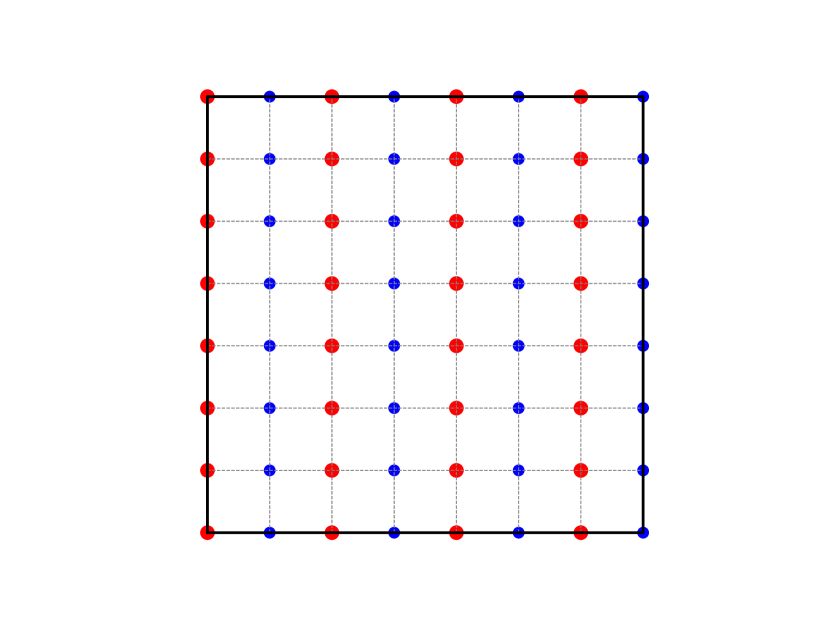
(a) Standard square

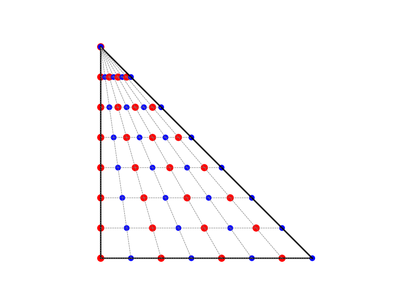
(b) Duffy’s transformation

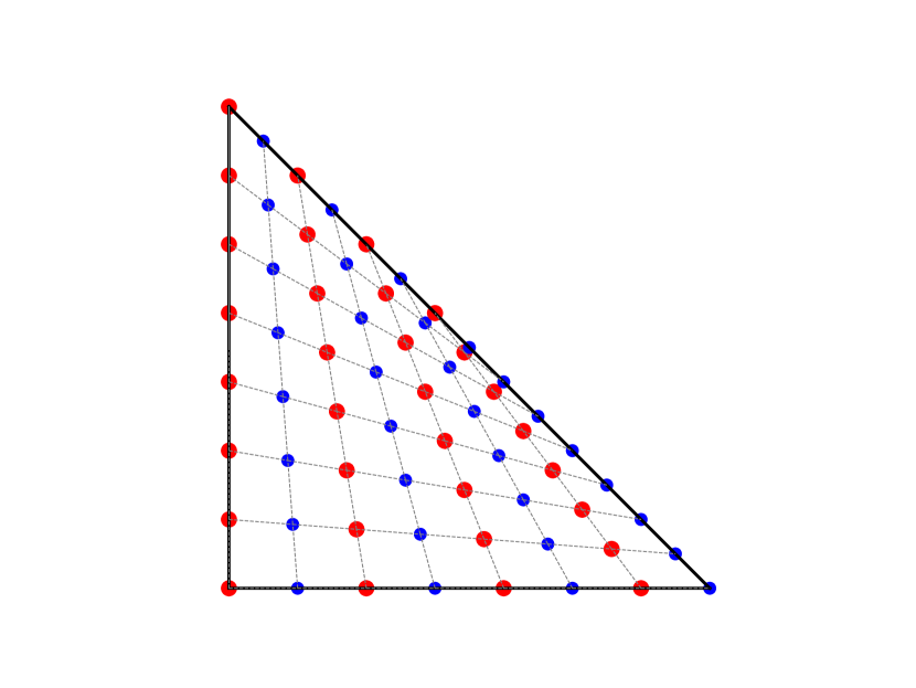
(c) Square-Squeezing

Figure 1: Bilinear square–simplex transformations: Deformations of equidistant grids, under Duffy’s transformation (b) and square-squeezing (c)

Figure 2: Construction of a surface parametrization over $\triangle_{2}$ by closest-point projection from a piecewise affine approximate mesh, and re-parametrization over the square $\Box_{2}$.

The quadrilateral re-parametrization enables interpolating the geometry functions $\varphi_{i}=\varrho_{i}\circ\sigma:\square_{2}\to\mathbb{R}^{3}$ by tensor-product polynomials, as we assert next.

3 Interpolation in the square

Our high-order format is based on interpolation in tensor-product Chebyshev–Lobatto nodes in the square $\square_{2}$. We start by defining:

Definition 2 (Lagrange polynomials MIP ; minterpy )

Let $n\in\mathbb{N}$ and $G_{2,n}=\oplus_{i=1}^{2}\mathrm{Cheb}_{n}$ be the tensorial Chebyshev–Lobatto grid, where $\mathrm{Cheb}_{n}=\left\{\cos\left(\frac{k\pi}{n}\right)\;:\;0\leq k\leq n\right\}$, indexed by a multi-index set $A_{2,n}=\{\alpha\in\mathbb{N}^{2}:\|\alpha\|_{\infty}\leq n\}^{2}$. For each $\alpha\in A_{2,n}$, the tensorial multivariate Lagrange polynomials are

$$L_{\alpha}(x)=\prod_{i=1}^{2}l_{\alpha_{i},i}(x)\,,\quad l_{j,i}(x)=\prod_{k=0,k\neq j}^{n}\frac{x_{i}-p_{k,i}}{p_{j,i}-p_{k,i}}\,.$$ (8)

The Lagrange polynomials are a basis of the polynomial space $\Pi_{2,n}=\mathrm{span}\{\mathrm{x}^{\alpha}=x_{1}^{\alpha_{1}}x_{2}^{\alpha_{2}}:\alpha\in A_{2,n}\}$ induced by $A_{2,n}$. Since the $L_{\alpha}$ satisfy $L_{\alpha}(p_{\beta})=\delta_{\alpha,\beta}$ for all $\alpha,\beta\in A_{2,n}$, $p_{\alpha}\in G_{2,n}$, we deduce that given a function $f:\square_{2}\to\mathbb{R}$, the interpolant $Q_{G_{2,n}}f\in\Pi_{2,n}$ of $f$ in $G_{2,n}$ is

$$Q_{G_{2,n}}f=\sum_{\alpha\in A_{2,n}}f(p_{\alpha})L_{\alpha}.$$ (9)

Definition 3 ($k^{\text{th}}$-order quadrilateral re-parametrization)

Given an $r$-regular quadrilateral re-parametrization $\varphi_{i}:\square_{2}\to S\,,\quad\varphi_{i}=\varrho_{i}\circ\sigma=\pi_{i}\circ\tau_{i}\circ\sigma\,,\quad i=1,\dots,K\,,$ mesh (7). We say that the mesh is of order $k$ if each element has been provided as a set of nodes $\{\varphi_{i}(p_{\alpha})\}_{\alpha\in A_{2,k}}$ sampled at $\{p_{\alpha}\}_{\alpha\in A_{2,k}}$.

This implies that on each element, we can approximate the $r$-regular quadrilateral re-parametrization maps through interpolation using the nodes $\{\varphi_{i}(p_{\alpha})\}_{\alpha\in A_{2,k}}$. This involves computing a $k^{\text{th}}$-order vector-valued polynomial approximation:

$$Q_{G_{2,k}}\varphi_{i}\left(\mathrm{x}\right)=\sum_{\alpha\in A_{2,k}}\varphi_{i}(p_{\alpha})L_{\alpha},\quad i=1,\ldots,K$$ (10)

The $r$-regular quadrilateral re-parametrization maps partial derivatives can be computed using numerical spectral differentiation trefethen2000spectral . These derivatives are then utilized to create an approximation of the metric tensor, $g_{i}$, for each element.

To obtain partial derivatives, forming the Jacobian matrix $DQ_{d,k}\varphi_{i}$ on the reference square $\square_{2}$, Kronecker products are employed. Let $D\in\mathbb{C}^{(k+1)\times(k+1)}$ be the one-dimensional spectral differentiation matrix trefethen2000spectral associated with Chebyshev–Lobatto nodes on the interval $[-1,1]$, and let $I\in\mathbb{C}^{(k+1)\times(k+1)}$ be the identity matrix. The differentiation matrices in the $x$ and $y$ directions on the reference square $\square_{2}$ are defined as follows:

$$D_{\mathrm{x}}Q_{G_{2,k}}\varphi_{i}=D\otimes I,\quad D_{\mathrm{y}}Q_{G_{2,k}}\varphi_{i}=I\otimes D,$$ (11)

where $D_{\mathrm{x}}Q_{G_{2,k}}\varphi_{i},D_{\mathrm{y}}Q_{G_{2,k}}\varphi_{i}\in\mathbb{C}^{(k+1)^{2}\times(k+1)^{2}}$.

Representing the Jacobian as $DQ_{d,k}\varphi_{i}=[D_{\mathrm{x}}Q_{d,k}\varphi_{i}\,|\,D_{\mathrm{y}}Q_{d,k}\varphi_{i}]$, the ingredients above realise the HOSQ, computing the surface integral as:

$$\int_{S}f\,dS \approx\sum_{i=1}^{K}\int_{\square_{2}}f(\varphi(\mathrm{x}))\sqrt{\det((DQ_{d,k}\varphi_{i}(\mathrm{x}))^{T}DQ_{d,k}\varphi_{i}(\mathrm{x}))}\,d\mathrm{x}$$ (12)

$$\approx\sum_{i=1}^{K}\sum_{\mathrm{p}\in P}\omega_{\mathrm{p}}f(\varphi_{i}(\mathrm{p}))\sqrt{\det((DQ_{d,k}\varphi_{i}(p))^{T}DQ_{d,k}\varphi_{i}(p))}\,,$$ (13)

where $\mathrm{p}\in P$, $\omega_{\mathrm{p}}\in\mathbb{R}^{+}$ can be the points and weights of any quadrature of $\square_{2}$ e.g. the Gauss-Legendre or Clenshaw-Curtis quadrature Xiang2012OnTC ; Trefethen2019 .

It is important to note that computing nodes and weights for a $n$-point Gauss-Legendre rule requires $\mathcal{O}(n^{2})$ operations (error analysis is given in zavalani2023highorder ), while the Clenshaw-Curtis method uses $\mathcal{O}(n\log n)$ operations with the Discrete Cosine Transform for evaluation. We estimate the error of the latter:

Theorem 3.1

Consider a $C^{r}$ surface $S$, where $r\geq 1$, with $r$-regular quadrilateral re-parametrization $\varphi_{i}:\square_{2}\to S$,

$$\varphi_{i}=\varrho_{i}\circ\sigma=\pi_{i}\circ\tau_{i}\circ\sigma,\quad i=1,\dots,K.$$

Let $\mathrm{p}\in P$, and $\omega_{\mathrm{p}}$ be the points and weights of the tensorial $(n+1)$-order Clenshaw-Curtis quadrature rule, $f:S\to\mathbb{R}$ be a function with absolutely continuous derivatives up to order $(r-1)$ and bounded variation $\|f^{(r)}\|_{T}=V<+\infty$, such that $f$ induces a negligible ”remainder of the remainder” elliott2011estimates . Then the integration error can be estimated as

$$\mathcal{E}_{f}=\sum_{i=1}^{K}\int_{\square_{2}}f(\varphi(\mathrm{x}))g_{i}\left(\mathrm{x}\right)d\mathrm{x}-\sum_{i=1}^{K}\sum_{\mathrm{p}\in P}\omega_{\mathrm{p}}f(\varphi_{i}(\mathrm{p}))g_{i}\left(\mathrm{p}\right)\leq\frac{128\tilde{V}}{15\pi r(n-r)^{r}},$$ (14)

where $g_{i}\left(\mathrm{x}\right)=\sqrt{\det((DQ_{d,k}\varphi_{i}(\mathrm{x}))^{T}DQ_{d,k}\varphi_{i}(\mathrm{x}))}$ and $\tilde{V}$ is defined as

$$\tilde{V}=\max_{i=1,\ldots,K}\max_{\alpha,\beta\leq r}\left\|\frac{\partial^{\alpha+\beta}}{\partial x^{\alpha}\partial y^{\beta}}\Big{(}f(\varphi_{i}(\mathrm{x}))g_{i}(\mathrm{x})\Big{)}\right\|_{T}\;\text{with}\;\|\xi\|_{T}=\left\|\frac{\xi^{\prime}}{\sqrt{1-x^{2}}}\right\|_{1}.$$ (15)

Proof

We denote $\psi(x,y):=f(\varphi(\mathrm{x}))g_{i}\left(\mathrm{x}\right)$ and

$$R^{(2)}_{n}[\psi]=I^{(2)}[\psi]-Q^{(2)}_{n}[\psi]$$ (16)

as the remainder of the exact integral and the $n+1$-order quadrature rule

$$I^{(2)}[\psi]=\int_{\square_{2}}\psi(x,y)\,dx\,dy,\quad Q^{(2)}_{n}[\psi]=\sum_{j=0}^{n}\sum_{i=0}^{n}\psi(x_{i},y_{j})\,w_{i}\,w_{j}\,.$$ (17)

For a bivariate function $\psi(x,y)$, $I_{x}[\psi]=\int_{-1}^{1}\psi(x,\cdot)\,dx$ denotes the integration with respect to the $x$ variable only, yielding a function of $y$. The subscript notation extends to $R_{n,x}[\psi]$ and $Q_{n,y}[\psi]$, and when replacing the roles of $x$ and $y$. Fubini’s theorem Brezis2010FunctionalAS implies:

$$I^{(2)}[\psi]=\int_{\square_{2}}\psi(x,y)\,dx\,dy=\int_{-1}^{1}I_{x}[\psi]\,dy=I_{y}[I_{x}[\psi]]\,.$$ (18)

Upon substitution into Eq. (18), we obtain

$$I^{(2)}[\psi] =I_{y}[R_{n,x}[\psi]+Q_{n,x}[\psi]]$$

$$=R_{n,y}[R_{n,x}[\psi]+Q_{n,x}[\psi]]+Q_{n,y}[R_{n,x}[\psi]+Q_{n,x}[\psi]]$$

$$=R_{n,y}[R_{n,x}[\psi]]+Q_{n,x}[R_{n,y}[\psi]]+Q_{n,y}[R_{n,x}[\psi]]+Q_{n,y}[Q_{n,x}[\psi]]$$ (19)

Following elliott2011estimates we assume the “remainder of a remainder” – first term in Eq. (3) to contribute negligibly to the error, enabling us to establish a sufficiently tight upper bound:

For large $n$, the quadrature rule approaches the value of the integral, i.e., $Q_{n,\beta}\approx I_{\beta}$ for $\beta=x,y$, we are left with:

$$I^{(2)}[\psi]\approx I_{x}[R_{n,y}[\psi]]+I_{y}[R_{n,x}[\psi]]+Q^{(2)}_{n}[\psi]\,.$$ (20)

Hence,

$$R^{(2)}_{n}[\psi]\leq I_{x}[R_{n,y}[\psi]]+I_{y}[R_{n,x}[\psi]],$$ (21)

As noted in Trefethen2019 , considering a function $\theta(x)$ defined on the interval $[-1,1]$, when computing $Q_{n}[\theta]$ using Clenshaw-Curtis quadrature for $\theta\in C^{r}$ and $\|\theta^{(r)}\|_{T}<V$ for a real finite value $V$, then for sufficiently large $n$, the subsequent inequality holds:

$$R_{n}[\theta]\leq\frac{32V}{15\pi r(n-r)^{r}}$$ (22)

Consequently, applying Eq. (22) to Eq. (21) yields

$$R^{(2)}_{n}[\psi]\leq\frac{32}{15\pi r(n-r)^{r}}[I_{x}[V_{y}(x)]+I_{y}[V_{x}(y)]]\,,$$ (23)

where $V_{y}(x)=\max_{y}\|\psi^{(r)}(x,y)\|_{T}$ and $V_{x}(y)=\max_{x}\|\psi^{(r)}(x,y)\|_{T}$ for fixed $x$ and $y$, respectively.

By utilizing the definition of the variation $\tilde{V}$ in Eq. (15), we are left with Eq. (14). Applying Clenshaw-Curtis quadrature leads to an error approximation for a 2D surface integral with an order of $\mathcal{O}\big{(}n^{-r}\big{)}$, where $n$ denotes the quadrature’s order.

4 Numerical experiments

We demonstrate the effectiveness of HOSQ-CC (utilizing Clenshaw-Curtis quadrature) for surface integration through two set of numerical examples. We provide the initial flat surface triangulations by using Persson and Strang’s algorithm Persson and subsequently enhance them to curved triangulations using Euclidean closest-point projections $\pi_{i}:T_{i}\to S$. Our implementation of HOSQ is part of a Python package surfpy . The examples and results of this manuscript using Dune-CurvedGrid are summarized and made available in the repository.

We compare HOSQ-CC with Dune-CurvedGrid integration algorithm (DCG) from the surface-parametrization module dune-curvedgrid CurvedGrid , part of the Dune finite element framework. As outlined in zavalani2024note , DCG performs total degree interpolation in uniform (equidistant midpoint-rule) triangle-nodes for interpolating the closest-point projection on each triangle, which makes it sensitive to Runge’s phenomenon (overfitting).

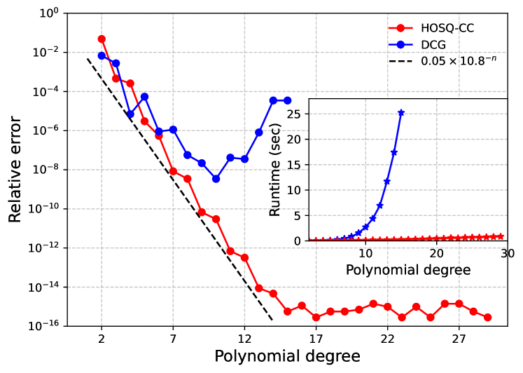
(a) Unit sphere

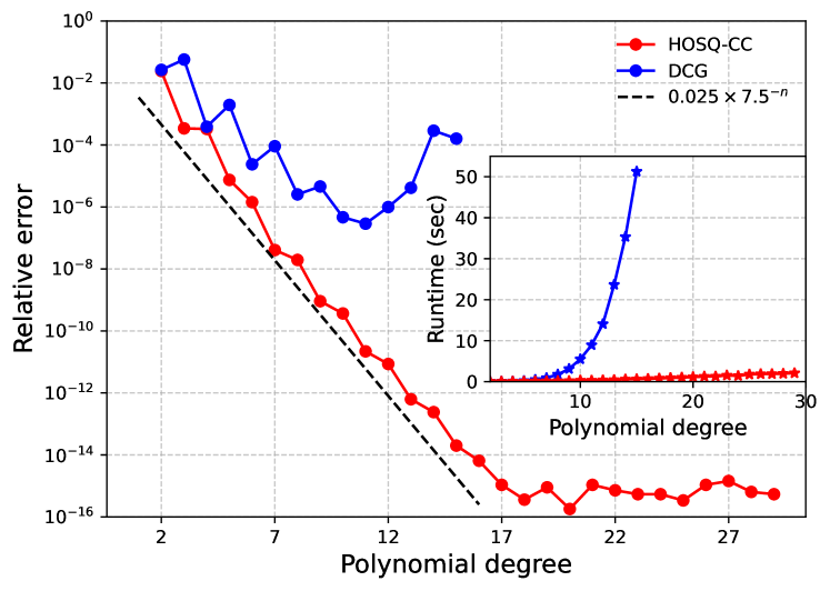
(b) Torus with radii $R=2$ and $r=1$

Figure 3: Relative errors and runtimes between DCG and HOSQ-CC computing the surface area of the unit sphere (3(a)) and torus (3(b)) respectively.

We start, by addressing integration tasks involving only constant integrands $f:S\to\mathbb{R}$.

Experiment 1 (Area computation)

We integrate $f=1$ over the unit sphere $\mathrm{S}^{2}$ and the torus $T^{2}_{r,R}$ with inner radius $r=1$ and outer radius $R=2$. The surface areas are given due to $4\pi r^{2}$ and $4\pi^{2}Rr$, respectively, enabling measuring the relative errors.

We choose initial triangulations of size $N_{\Delta}=124$ for the sphere and of size $N_{\Delta}=256$ for the torus and apply Clenshaw-Curtis quadratureTrefethen2019 , with a degree matching the geometry approximation. We use symmetric Gauss quadrature on a simplex with a matching degree for the geometry approximation in the case of DCG.

HOSQ-CC exhibits stable convergence to machine precision with exponential rates, $0.05\times 10.8^{-n}$ and $0.025\times 7.5^{-n}$ fitted for the sphere and torus, respectively, in accordance with the predictions from Theorem 3.1. In contrast, DCG becomes unstable for orders larger than $\deg=10$. We interpret the instability as the appearance of Runge’s phenomenon caused by the choice of midpoint-triangle-refinements yielding equidistant interpolation nodes for DCG.

In terms of execution time, the Python implementation of HOSQ-CC, empowered by spectral differentiation, outperforms the $\text{C}++$ implementation of DCG. Importantly, experimental findings reveal that DCG encounters constraints for $\deg\geq 15$, attributable to the formation of a singular matrix during the basis computation.

Experiment 2 (Gauss-Bonet validation)

We consider the Gauss curvature as a non-trivial integrand. Due to the Gauss–Bonnet theorem spivak1999 , integrating the Gauss curvature over a closed surface yields

$$\int_{S}K_{\mathrm{Gauss}}\,dS=2\pi\chi\left(S\right)\,,$$ (24)

where $\chi\left(S\right)$ denotes the Euler characteristic of the surface. Here, we consider:

1)	Dziuk’s surface	$(x-z^{2})^{2}+y^{2}+z^{2}-1=0$
2)	Double torus	$\big{(}x^{2}+y^{2})^{2}-x^{2}+y^{2}\big{)}^{2}+z^{2}-a^{2}=0$ , $a\in\mathbb{R}\setminus\{0\}$

The Gauss curvature is computed symbolically from the implicit surface descriptions using Mathematica 11.3, enabling measuring errors of DCG and HOSQ-CC when integrating the Gauss curvature. We maintain the experimental design outlined in Experiment 1 and display error plots based on the polynomial degree in Fig.4 and Fig.5.

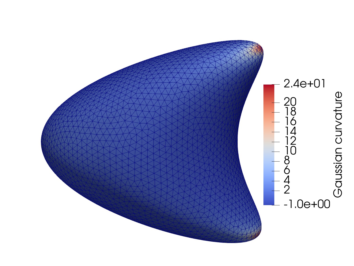
(a) Dziuk’s surface with $8088$ triangles

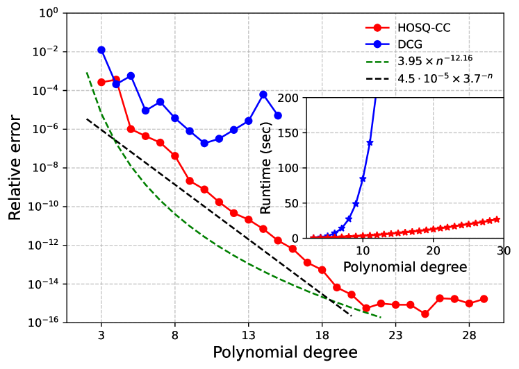
(b) Integration errors and and runtimes

Figure 4: Gauss-Bonnet validation for Dziuk’s surface.

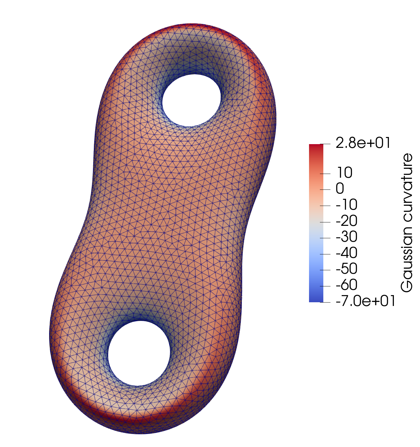
(a) Double torus, with $8360$ triangles and $a=0.2$

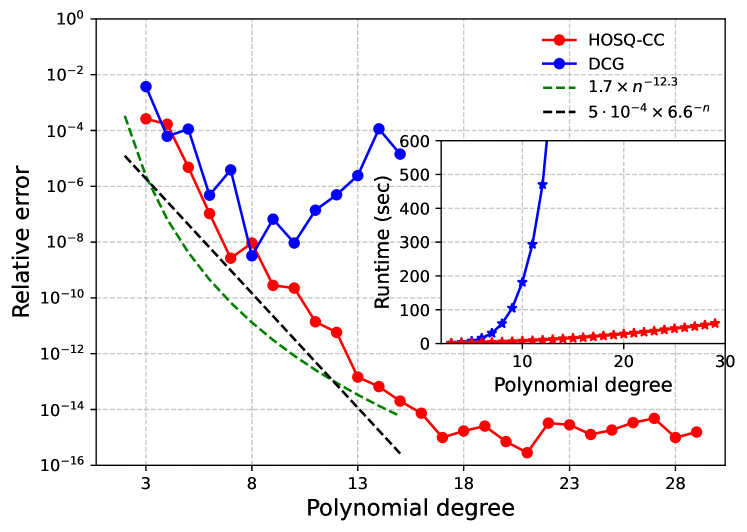
(b) Integration errors and and runtimes

Figure 5: Gauss-Bonnet validation for a double torus.

The HOSQ-CC consistently exhibits exponential convergence to the accurate value $2\pi\chi(S)$ with exponential rates, $4.5\cdot 10^{-5}\times 3.7^{-n}$ and $5\cdot 10^{-4}\times 6.6^{-n}$ fitted for the for the Dziuk’s surface and the double torus, respectively. The best fit of an algebraic rate, $3.95\times n^{-12.16}$ for the Dziuk’s surface and $1.7\times n^{-12.3}$ for the double torus, does not assert rapid convergence. As the order increases, the error in HOSQ-CC tends to stabilize near the level of machine precision. In contrast, DCG fails to achieve machine-precision approximations across all cases and becomes unstable for degrees $k\geq 10$. In terms of execution time, once more, HOSQ-CC, empowered by spectral differentiation, outperforms DCG.

5 Conclusion

The present HOSQ integration approach, utilizing the innovative square-squeezing transformation excels in speed, accuracy, and robustness for integration task on complex geometries, suggesting its application potential for triangular spectral element methods (TSEM) karniadakis2005spectral ; heinrichs2001spectral and fast spectral PDE solvers on surfaces fortunato2022high .

References

- [1] A. Bonito and R. H. Nochetto. Geometric Partial Differential Equations — Part I. Elsevier, 2020.
- [2] H. Brezis. Functional analysis, sobolev spaces and partial differential equations. 2010.
- [3] Q. Chen and I. Babuška. Approximate optimal points for polynomial interpolation of real functions in an interval and in a triangle. Computer Methods in Applied Mechanics and Engineering, 128(3):405–417, 1995.
- [4] M. G. Duffy. Quadrature over a pyramid or cube of integrands with a singularity at a vertex. SIAM Journal on Numerical Analysis, 19:1260–1262, 1982.
- [5] G. Dziuk and C. M. Elliott. Finite element methods for surface PDEs. Acta Numerica, 22:289–396, 2013.
- [6] D. Elliott, P. R. Johnston, and B. M. Johnston. Estimates of the error in gauss–legendre quadrature for double integrals. Journal of Computational and Applied Mathematics, 236(6):1552–1561, 2011.
- [7] D. Fortunato. A high-order fast direct solver for surface PDEs. arXiv preprint arXiv:2210.00022, 2022.
- [8] S. J. Gregg, K. S. W. Sing, and H. W. Salzberg. Adsorption surface area and porosity. Journal of The Electrochemical Society, 114(11):279, nov 1967.
- [9] M. Hecht, K. Gonciarz, J. Michelfeit, V. Sivkin, and I. F. Sbalzarini. Multivariate interpolation in unisolvent nodes–lifting the curse of dimensionality. arXiv preprint arXiv:2010.10824, 2020.
- [10] W. Heinrichs and B. I. Loch. Spectral schemes on triangular elements. Journal of Computational Physics, 173(1):279–301, 2001.
- [11] U. Hernandez Acosta, S. Krishnan Thekke Veettil, D. Wicaksono, and M. Hecht. minterpy – Multivariate interpolation in Python. https://github.com/casus/minterpy, 2021.
- [12] G. E. Karniadakis, G. Karniadakis, and S. Sherwin. Spectral/ element methods for computational fluid dynamics. Oxford University Press, 2005.
- [13] J.-O. Lachaud. Convergent geometric estimators with digital volume and surface integrals. In Discrete Geometry for Computer Imagery, pages 3–17. Springer, 2016.
- [14] P.-O. Persson and G. Strang. A simple mesh generator in MATLAB. SIAM Review, 46(2):329–345, 2004.
- [15] S. Praetorius and F. Stenger. Dune-CurvedGrid – a Dune module for surface parametrization. Archive of Numerical Software, page Vol. 1 No. 1 (2022), 2022.
- [16] J. C. Riviere and S. Myhra. Handbook of surface and interface analysis: methods for problem-solving. CRC press, 2009.
- [17] M. Spivak. A Comprehensive Introduction to Differential Geometry, volume 1. Publish or Perish Incorporated, 1999.
- [18] M. A. Taylor and B. Wingate. A generalized diagonal mass matrix spectral element method for non-quadrilateral elements. Applied Numerical Mathematics, 33(1-4):259–265, 2000.
- [19] L. N. Trefethen. Spectral Methods in MATLAB. Society for Industrial and Applied Mathematics, 2000.
- [20] L. N. Trefethen. Approximation theory and approximation practice, volume 164. SIAM, 2019.
- [21] S. Xiang and F. A. Bornemann. On the convergence rates of gauss and clenshaw-curtis quadrature for functions of limited regularity. SIAM J. Numer. Anal., 50:2581–2587, 2012.
- [22] G. Zavalani, O. Sander, and M. Hecht. High-order integration on regular triangulated manifolds reaches super-algebraic approximation rates through cubical re-parameterizations. arXiv preprint arXiv:2311.13909, 2023.
- [23] G. Zavalani, E. Shehu, and M. Hecht. A note on the rate of convergence of integration schemes for closed surfaces. Computational and Applied Mathematics, 43(2):1–17, 2024.
- [24] Q. Zhou and P. Somasundaran. Surface and Interfacial Tension: Measurement, Theory, and Applications. Surfactant Science Series, volume 119. ACS Publications, 2005.