Bridging Quantum Computing and Differential Privacy: A Survey on Quantum Computing Privacy

Abstract.

Quantum computing has attracted significant attention in areas such as cryptography, cybersecurity, and drug discovery. Due to the advantage of parallel processing, quantum computing can speed up the response to complex challenges and the processing of large-scale datasets. However, since quantum computing usually requires sensitive datasets, privacy breaches have become a vital concern. Differential privacy (DP) is a promising privacy-preserving method in classical computing and has been extended to the quantum domain in recent years. In this survey, we categorize the existing literature based on whether internal inherent noise or external artificial noise is used as a source to achieve DP in quantum computing. We explore how these approaches are applied at different stages of a quantum algorithm (i.e., state preparation, quantum circuit, and quantum measurement). We also discuss challenges and future directions for DP in quantum computing. By summarizing recent advancements, we hope to provide a comprehensive, up-to-date overview for researchers venturing into this field.

1. Introduction

Quantum computing is an emerging technology based on the principles of quantum mechanics. With the parallel processing from quantum attributes, quantum computing has been more advantageous than the current computing pattern in some areas, such as drug discovery (cao2018potential, ), materials engineering (de2021materials, ), and financial analysis (orus2019quantum, ). Quantum algorithms are a set of tailored instructions for quantum computing, aimed at exponential acceleration to solve some particular problems (e.g. Shor’s algorithm (shor1994algorithms, ), Grover’s algorithm (grover1996fast, ), and HHL algorithm (harrow2009quantum, )). As a typical class of quantum algorithms, variational quantum algorithms (VQA) (cerezo2021variational, ) include popular fields of quantum machine learning (QML), quantum approximate optimization algorithm (QAOA) (farhi2014quantum, ), and variational quantum eigensolver (VQE) (peruzzo2014variational, ). However, these applications of quantum algorithms often require sensitive datasets, such as DNA sequence data (ur2023quantum, ), making user privacy increasingly important.

Table 1. Summary of notations.

Symbol	Definition
$\mathcal{A}$	a quantum algorithm
$\mathcal{I}$	input of quantum algorithm
$\mathcal{O}$	output of quantum algorithm
$\mathcal{H}$	Hilbert space
$\mathcal{E}$	quantum channel (super-operator)
$\mathcal{E}^{\dagger}$	dual form of quantum channel $\mathcal{E}$
$\mathcal{N}$	noise channel
$\mathbb{I}$	identity matrix
$n$	the number of qubits
$\kappa$	quantum kernel
$n_{\mathrm{shot}}$	the number of shots
$x$	data point (vector) from classical dataset
$|i\rangle$	a set of orthonormal basis in Hilbert space
$|\rho\rangle,|\sigma\rangle$	pure quantum state
$\rho,\sigma$	mixed quantum state
$U$	quantum gate
$M$	a set of measurements
$E$	a Kraus operator
$\tau(\cdot,\cdot)$	distance metric between states
$\mathrm{Tr}(\cdot)$	trace of a matrix
$P(\cdot)$	the power set of a set
$\epsilon$	privacy budget
$\delta$	fault tolerance rate
$p$	probability of gate flipping in Pauli channels
$\alpha$	factor of hockey-stick divergence
$\beta$	upper bound of contraction coefficient
$\gamma$	error probability of amplitude damping channel
$\lambda$	error probability of phase damping channel

Differential privacy (DP), proposed by Dwork et al.  (dwork2014algorithmic, ), is a promising approach to address the problem of data leakage in traditional computing. It guarantees that the addition or reduction of an individual’s information has a negligible effect on the algorithm’s result, thus protecting the individual’s information. DP has a rigorous mathematical proof and usually uses $\epsilon$ to indicate the degree of privacy protection. Recently, DP has been introduced to the quantum domain to protect user privacy in quantum computing (zhou2017differential, ; guan2023detecting, ; hirche2023quantum, ). A common idea is to follow the approach of implementing classical DP, i.e., artificially adding noise to realize DP in quantum computing. Senekane et al. (senekane2017privacy, )first applied the classical DP mechanism to a classical dataset by introducing discrete Laplace noise. The resulting output is subsequently converted to a quantum state as a way to protect the quantum machine learning model. Moreover, in recent years, the inherent noise generated by quantum computing has also been subtly considered as one of the sources for realizing DP (zhou2017differential, ; guan2023detecting, ; hirche2023quantum, ). This inherent noise is generated in quantum devices due to undesirable or imperfect interactions in the physical environment. Quantum computing is in the era of “Noise Intermediate Quantum Quantum (NISQ)”, so the inherent noise cannot be eliminated and is usually regarded as a hindrance to quantum computing. However, Zhou’s work (zhou2017differential, ) first suggests how to skillfully model inherent noise (i.e., depolarization, amplitude damping, and phase damping) as a privacy mechanism for quantum computation, each with a corresponding privacy budget calculation. It shows that while inherent noise in quantum devices poses computational difficulties, it also naturally allows for a degree of DP in quantum computation.

From the preceding discussion, there are currently two ways to implement DP in quantum computing: adding external noise or utilizing inherent noise. So, we categorize the existing literature by discussing these two ways separately in each component of the quantum algorithm (i.e., state preparation, quantum circuit, and quantum measurement). We also summarize some challenges and future directions of DP in quantum computing.

The remainder of the paper is organized as follows. In Section 2, we first review some notions of quantum theory including the basic concepts of quantum computation, quantum algorithm, and quantum noise. Then we introduce DP and its quantum extension. In Section 3, we discuss how the inherent noise and external noise of the quantum algorithm enable DP in quantum computing. Challenges and future potential directions are provided in Section 4.

2. Preliminaries

In this section, we first introduce some basic concepts of quantum computation and elaborate on how a quantum algorithm works. Then, we briefly formalize the definition of DP and extend it to the quantum version. Finally, we give a case of how to obtain DP using quantum noise. Throughout this survey, we will use the following notations as shown in Tab. 1.

2.1. Qubits, quantum gates and circuits

The atom unit of quantum computation is quantum bits (qubits). Qubits could be described as the linear combination of a set of computational basis state vectors (i.e. $|0\rangle$ and $|1\rangle$) in $2^{n}$-dimensional Hilbert space $\mathcal{H}$, where $n$ is the number of qubits. Quantum computing is an algorithmic process of quantum states characterized by qubits and is implemented on quantum hardware through quantum circuits consisting of wires and quantum gates.

Quantum gates are mathematically represented by unitary matrices $U$. For any quantum logic gate, it satisfies that $U^{\dagger}=U^{-1}$, where $U^{\dagger}$ is the adjoint (conjugate transpose) of $U$. This property ensures that it is logically linear, reversible, and non-trivial. The most basic quantum gates are 1-qubit gates, such as Pauli gate ($I$, $X$, $Y$, $Z$), Hadamard gate ($H$), and rotation gate ($R_{x}$, $R_{y}$, $R_{z}$),

(1) $$I=\begin{pmatrix}1&0\\ 0&1\end{pmatrix}\quad X=\begin{pmatrix}0&1\\ 1&0\end{pmatrix}\quad Y=\begin{pmatrix}0&-i\\ i&0\end{pmatrix}\quad Z=\begin{pmatrix}1&0\\ 0&-1\end{pmatrix}\quad H=\frac{1}{\sqrt{2}}\begin{pmatrix}1&1\\ 1&-1\end{pmatrix},$$

$$R_{x}(\theta)=\begin{pmatrix}\cos{\frac{\theta}{2}}&-i\sin{\frac{\theta}{2}}\\ -i\sin{\frac{\theta}{2}}&\cos{\frac{\theta}{2}}\end{pmatrix}\quad R_{y}(\theta)=\begin{pmatrix}\cos{\frac{\theta}{2}}&-\sin{\frac{\theta}{2}}\\ \sin{\frac{\theta}{2}}&\cos{\frac{\theta}{2}}\end{pmatrix}\quad R_{z}(\theta)=\begin{pmatrix}\exp(-i\frac{\theta}{2})&0\\ 0&\exp(i\frac{\theta}{2})\end{pmatrix}.$$

The rotation gate is usually considered as the main component of a variational circuit with the learnable rotation angle $\theta$. More complex quantum gates are 2-qubit Controlled-U gates, which induce entanglement between qubits, such as $CX$, $CZ$, and $CR_{x}$,

$$CX=\begin{pmatrix}1&0&0&0\\ 0&1&0&0\\ 0&0&0&1\\ 0&0&1&0\end{pmatrix}\quad CZ=\begin{pmatrix}1&0&0&0\\ 0&1&0&0\\ 0&0&1&0\\ 0&0&0&-1\end{pmatrix}\quad CR_{x}(\theta)=\begin{pmatrix}1&0&0&0\\ 0&1&0&0\\ 0&0&\cos{\frac{\theta}{2}}&-i\sin{\frac{\theta}{2}}\\ 0&0&-i\sin{\frac{\theta}{2}}&\cos{\frac{\theta}{2}}\end{pmatrix}.$$

More details can be found in the textbook (nielsen2010quantum, ).

A quantum circuit is a set of ordered collections of wires and quantum gates, which is utilized to evolve quantum states. For an input $n$-qubit state $\rho$ and a quantum circuit $\mathcal{E}=U_{d}\dots U_{1}$, where $U_{i}$ is donated as a quantum gate and $d$ is the depth of circuit $\mathcal{E}$, the output of evolution is

(2) $$\mathcal{E}(\rho)=U_{d}(\dots(U_{1}\rho U_{1}^{\dagger})\dots)U_{d}^{\dagger}.$$

2.2. Quantum algorithm

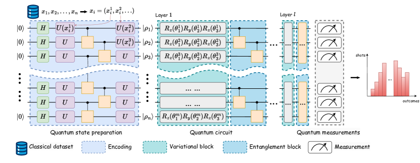
Figure 1. Variational quantum algorithm (VQA), take QML model as an example. The classical part is omitted.

Quantum algorithms are a set of tailored instructions for quantum computing, aimed at exponential acceleration to solve some particular problems (e.g. Shor’s algorithm for identifying the prime factors of an integer and HHL algorithm for solving linear equations). A common type of quantum algorithm, such as variational quantum algorithm (VQA) (cerezo2021variational, ), is composed of initial quantum states, the trainable quantum circuit, and quantum measurements. As illustrated in Fig. 1, a trainable quantum circuit is fed with quantum data or classical data encoded by quantum encoding, and its outputs are collapsed into classical information by quantum measurements.

1) State preparation

Classical datasets are readily available and well-established, but not directly suitable for performing VQA. Hence VQA typically requires state preparation, i.e., initializing classical datasets into state vectors in Hilbert space via quantum encoding. Let $x=(x_{1},\dots,x_{n})$ be a classical dataset, where each $x_{i}$ is a vector. Let $\phi$ be a quantum encoding method, initial states $\rho$ can be realized via

(3) $$\rho\leftarrow\phi(x)=|\phi(x)\rangle\langle\phi(x)|.$$

Several common quantum encodings are summarized in Tab. 2.

Table 2. Common approaches for quantum encoding.

Encoding $\mathcal{E}_{\mathrm{en}}$	mapping $\phi$	kernel $\kappa$
Basic Encoding	$x\mapsto\frac{1}{\sqrt{n}}\sum^{n}_{i=1}|x_{i}\rangle$	$\delta_{x_{i},x_{j}}$
Amplitude Encoding	$x\mapsto\sum^{n}_{i=1}\frac{x_{i}}{\parallel x\parallel}|i\rangle$	$|x_{i}^{\top}x_{j}|^{2}$
Angle Encoding	$x\mapsto\bigotimes^{n}_{i=1}R(x_{i})|0\rangle$	$\prod^{n}_{k=1}|\cos(x_{i}^{k}-x_{j}^{k})|^{2}$

If $x_{i}$ is a binary string, it is more eligible to adopt basic encoding, characterized by a uniform superposition of an orthonormal basis. For a complex value $x_{i}\in\mathbb{C}^{d}$, amplitude encoding is the better choice, though it is almost impossible to implement in the NISQ era because of its requirement for deeper and more complex circuits. Angle encoding is easier to implement and only requires one rotation gate on each wire, with $x_{i}\in[0,2\pi]^{d}$ as angles.

Additionally, similar to kernel methods, the notion of quantum kernel is rose in  (schuld2021supervised, , Definition 2), that a quantum kernel $\kappa$ is the inner product between encoding vectors of two datasets

(4) $$\kappa(x,y)=|\langle\phi(x)|\phi(y)\rangle|^{2},\quad\mbox{where}\ x,y\in\mathcal{D}.$$

2) Quantum circuit

As previously introduced, the quantum circuit is the core computational component of the quantum algorithm. The input of the circuit is usually a pure state, which is a complex unit vector in $2^{n}$-dimensional Hilbert space $\mathcal{H}$, written in Dirac notation as

$$|\rho\rangle=\sum_{i}^{n}\alpha_{i}|i\rangle,$$

where $|i\rangle$ is an orthonormal basis in $\mathcal{H}$ and $\sum_{i}\alpha_{i}=1$. For example, as for a 1-qubit quantum system, a pure state in 2-dimensional Hilbert space can be represented as $|\rho\rangle=\alpha|0\rangle+\beta|1\rangle$, where $|0\rangle=[1,0]^{\top},|1\rangle=[0,1]^{\top}$ and $\alpha^{2}+\beta^{2}=1$.

The circuit performed on naturally noisy hardware turns a pure state into a mixed state as output, which is mathematically modeled as a $n\times n$-dimensional density matrix

$$\psi=\sum_{k}p_{k}|\rho_{k}\rangle\langle\rho_{k}|,$$

where $p_{k}$ is the probability that $\psi$ collapses into $|\rho_{k}\rangle$ and $\sum_{k}p_{k}^{2}=1$.

3) Quantum measurements

The output of the quantum algorithm is determined by the probabilistic occurrence of quantum states, resulting from measurements over superposition. Therefore, the final answer to the algorithmic flow is a discrete probabilistic distribution, as illustrated in the last part in Fig. 1. The x-axis is all the possible outcomes of measurements and the y-axis is the number of shots.

For example, if the output of a circuit is $\rho$ and a set of measurements are represented by $n\times n$ positive semi-definite matrices $\{M_{i}\}_{i\in\mathcal{O}}$, where $\mathcal{O}$ is the set of all possible outcomes, then $p_{i}=\mathrm{Tr}(M_{i}\rho)$ is the probability that the outcome of the measurement is $i$.

2.3. The formulation of DP and its quantum extension

Differential privacy (DP) (dwork2006calibrating, ) provides a quantifiable privacy guarantee by ensuring that subtle changes in datasets do not affect the probability of any outcome. We first review some basic notions of classical DP before giving the formulation.

Definition 1 (neighboring datasets (dwork2014algorithmic, )).

For two datasets $x,x^{\prime}\in\mathcal{D}$, we call them neighbors if the following inequality holds:

(5) $$d(x,x^{\prime})\leq 1,$$

where function $d(\cdot)$ calculates the Manhattan or Euclidean distance between datasets.

Here, neighbors $x$ and $x^{\prime}$ differ by one entry, which originally describes the subtle change in datasets. Then, the following definition of global sensitivity represents an upper bound of a function (or query) on neighbors.

Definition 2 (global sensitivity (dwork2014algorithmic, )).

For two neighboring datasets $x,x^{\prime}\in\mathcal{D}$, and a function (or query) $f:\mathcal{D}\rightarrow\mathcal{S}$, global sensitivity $\Delta f$ is the least upper bound of the distance between neighbors with $f$ applied. Taking the Manhattan distance as an example:

(6) $$\Delta f=\underset{x,x^{\prime};d(x,x^{\prime})\leq 1}{\max}\left\|f(x)-f(x^{\prime})\right\|_{1}.$$

Definition 2 indicates the maximum change in the function (or query)’s output when its input changes slightly (by addition or removal of one entry). Roughly speaking, a higher sensitivity requires a greater need for the amount of randomization to ensure DP.

The DP property of datasets characterizes the indistinguishability of query outputs under the neighboring setting. Using Def. 1 and Def. 2, the formal definition of DP can be obtained, as proposed in a series of articles published by Dwork et al.  (dwork2006differential, ; dwork2006calibrating, ; dwork2010boosting, ; dwork2014algorithmic, ).

Definition 3 ($(\epsilon,\delta)$-DP).

A randomized algorithm $\mathcal{M}$ satisfies $(\epsilon,\delta)$-DP if for any pair of datasets $x,x^{\prime}\in\mathcal{D}$ that are neighbors and all possible outcomes $S$, then we have

(7) $$\mathrm{Pr}[\mathcal{M}(x)\in\mathcal{S}]\leq\exp(\epsilon)\cdot\mathrm{Pr}[\mathcal{M}(x^{\prime})\in\mathcal{S}]+\delta,$$

where Eq. (7) holds with probability at least $1-\delta$. We define $\mathcal{M}$ to be $\epsilon$-DP by setting $\delta=0$.

In classical scenarios, a DP mechanism is usually realized by applying a perturbation directly onto the input data or query output, such as the Laplace mechanism and the Gaussian mechanism, or by flipping a biased coin such as the randomized response mechanism (RR).

Definition 4 (additive noise mechanism).

Given a function (or query) $f:\mathcal{D}\rightarrow\mathcal{S}$ and a noise distribution $\mathcal{N}$, then the additive noise mechanism could be described as

(8) $$\mathcal{M}_{\mathcal{N}}(x,f(\cdot),\epsilon,\delta)=f(x)+\mathcal{N}.$$

Definition 4 instantiates to Laplace mechanism when $\mathcal{N}\sim\mathrm{Lap}(0,\sigma=\Delta f/\epsilon)$, where $\mathrm{Lap}(x,\mu,\sigma)=\frac{1}{2\sigma}\exp(-\frac{|x-\mu|}{\sigma})$, and Gaussian mechanism when $\mathcal{N}\sim\mathrm{Gau}(0,\sigma=\sqrt{2\ln(1.25/\delta)}\cdot\Delta f/\epsilon)$, where $\mathrm{Gau}(x,\mu,\sigma)=\frac{1}{\sqrt{2\pi}\sigma}\exp(-\frac{(x-\mu)^{2}}{2\sigma^{2}})$. $\epsilon$ and $\delta$ are privacy parameters introduced in Def. 3 and $\Delta f$ is global sensitivity introduced in Def. 2.

In contrast to directly adding noise on a range of one dataset, the randomized response mechanism (erlingsson2014rappor, ) introduces randomization by flipping coins, creating privacy about the true query answer response to one data point.

Definition 5 (randomized response mechanism).

Supposed that a function (or query) $f:\mathcal{D}\rightarrow\mathcal{S}$ returns a true answer with a probability of the coin being heads of $\frac{\exp(\epsilon)}{\exp(\epsilon)+1}$, where $\epsilon\in[0.\infty]$, then the randomized response mechanism (RR) could be described as

(9) $$\mathcal{M}_{\mathrm{RR}}(x,f(\cdot),\epsilon)=\frac{\exp(\epsilon)}{\exp(\epsilon)+1}f(x)+\frac{1}{\exp(\epsilon)+1}\tilde{f}(x),$$

where $\tilde{f}(\cdot)$ returning a random answer.

The implementation of the randomized response mechanism implies a stronger version of DP, namely local differential privacy (LDP).

Definition 6 ($(\epsilon,\delta)$-LDP).

A randomized algorithm $\mathcal{M}$ satisfies $(\epsilon,\delta)$-LDP if for any pair of datapoints $x,x^{\prime}\in\mathcal{D}$ and the possible outcome $y$, then we have

(10) $$\mathrm{Pr}[\mathcal{M}(x)=y]\leq\exp(\epsilon)\cdot\mathrm{Pr}[\mathcal{M}(x^{\prime})=y]+\delta,$$

where Eq. (10) holds with probability at least $1-\delta$. We define $\mathcal{M}$ to be $\epsilon$-LDP by setting $\delta=0$.

Notably, LDP considers the information that a sample is distinguished from another sample as private, rather than a handful of samples, which means that there is no need to impose Def. 1 constraints on it.

Table 3. Distance metrics.

Reference (cites)	Metric	Description
Zhou et al. (zhou2017differential, )	bounded trace distance	Two close quantum states are measured by trace distance $\left\|\rho-\sigma\right\|_{\rm{tr}}=\rm{Tr}(|\rho-\sigma|)/2$, bounded with $d$, that is $\tau(\rho,\sigma)=\left\|\rho-\sigma\right\|_{\rm{tr}}\leq d$.
Gong et al. (gong2022enhancing, )	normalized Hamming distance	Two quantum states that encoded from initial state $|0\rangle^{\otimes n}$ can be represented as $\rho=e_{\rho}|0\rangle^{\otimes n}$ and $\sigma=e_{\sigma}|0\rangle^{\otimes n}$, then the normalized Hamming distance between states is $\tau_{\mathrm{ham}}(\rho,\sigma)=1/n\sum^{n}_{i=1}\mathbf{1}[e_{\rho}^{i}\neq e_{\sigma}^{i}]$, bounded with $d$, that is $\tau_{\mathrm{ham}}(\rho,\sigma)\leq d$.
Hirche et al. (hirche2023quantum, )	Wasserstein distance of order $1$	The distance metric is the Wasserstein distance of order 1 $W_{1}(\rho,\sigma)={\sup}_{\{M_{i}\}_{i\in\mathcal{O}}}\mathrm{Tr}(M_{i}\rho-M_{i}\sigma)$, bounded with $d$, that is, $W_{1}(\rho,\sigma)\leq d$.
Aronson et al. (aronson2019gentle, )	reachability by single-register operation	Two quantum states are neighbors if each of both reaches either ($\sigma$ from $\rho$, or $\rho$ from $\sigma$) by performing a super-operator on a single qubit only.
Angrisani et al. (angrisani2023unifying, )	$(\mathcal{L},d)$-neighboring	Two quantum states are $(\mathcal{L},d)$-neighboring if $\exists\ell\in\mathcal{L}$ and $\mathcal{L}\subset P([n])$, there have $\mathrm{Tr}(M_{\ell}\rho)=\mathrm{Tr}(M_{\ell}\sigma)\wedge\left\|\rho-\sigma\right\|_{\rm{tr}}\leq d$. If $\mathcal{L}=\{[n]\}$, it is equivalent to trace distance bounded with $d$. If $\mathcal{L}=1$ and $d=1$, it recovers the metric that reachability by single register operation.
Tomamichel (tomamichel2015quantum, )	purified distance	For two quantum states $\rho,\sigma$, their purified distance is defined as the minimal trace distance between purifications of the states, that is $P(\rho,\sigma):=\sqrt{1-F_{*}(\rho,\sigma)}$ where generalized fidelity $F_{*}(\rho,\sigma)=(\mathrm{Tr}(|\sqrt{\rho}\sqrt{\sigma}|)+\sqrt{(1-\mathrm{Tr}(\rho))(1-\mathrm{Tr}(\sigma))})^{2}$.

In recent years, researchers have attempted to transfer classical mechanisms to quantum scenarios, consequently generalizing Def. 3 into the quantum domain. First, quantum states are targeted as DP objects rather than databases (dwork2006differential, ), query results (dwork2006calibrating, ) or gradients (abadi2016deep, ). Second, various distance metrics are introduced to measure the neighboring relationship between quantum states, as the setting of Def. 1. Shown in Tab. 3, Zhou et al. (zhou2017differential, ) first state their definition of the quantum version of “neighboring”. The closeness of two close quantum states is measured by bounded trace distance, where states are mathematically modeled as density matrices. Aronson and Rothblum introduced a classical-like metric (aronson2019gentle, ), where two quantum states are neighbors if any state can reach another state ($\sigma$ from $\rho$, or $\rho$ from $\sigma$) by performing a channel on a single qubit. If quantum states are represented in a product way, Gong et al. (gong2022enhancing, ) present normalized Hamming distance to measure the closeness between states. Inspired by the work from  (de2021quantum, ), Hirche et al. (hirche2023quantum, ) and Angrisani et al. (angrisani2023unifying, ) propose the quantum Wasserstein distance instead of trace distance to obtain tighter privacy upper bounds. A generalized quantum neighboring relationship is presented in (angrisani2023unifying, ), with these previous metrics, i.e. bounded trace distance and reachability by single register operation as its two particular cases, respectively. The formal definition of neighboring quantum states is as follows.

Definition 7 (neighboring quantum states).

For two quantum states $\rho,\sigma\in\mathcal{H}$, we call them neighbors within distance $d$ if the following inequality holds:

(11) $$\tau(\rho,\sigma)\leq d,$$

where $\tau(\cdot)$ is denoted as a kind of distance metric.

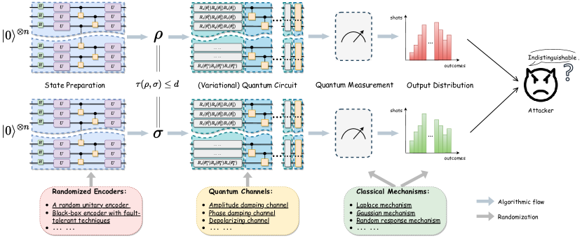
Figure 2. Quantum differential privacy of quantum algorithm.

Finally, these work (zhou2017differential, ; aronson2019gentle, ; hirche2023quantum, ; angrisani2023unifying, ) formalize the mathematical meaning of quantum differential privacy (QDP) and clarify the following definition.

Definition 8 ($(\epsilon,\delta)$-QDP).

A noisy quantum algorithm $\mathcal{A}=(\mathcal{E},\{M_{i}\}_{i\in\mathcal{O}})$ satisfies $(\epsilon,\delta)$-QDP if, for any pair of input states $\rho,\sigma$ that are neighbors within distance $d$ and any measurement output $\mathcal{O}$, we have

(12) $$\sum_{i\in\mathcal{O}}\mathrm{Tr}[M_{i}\mathcal{E}(\rho)]\leq\exp{(\epsilon(d))}\cdot\sum_{i\in\mathcal{O}}\mathrm{Tr}[M_{i}\mathcal{E}(\sigma)]+\delta,$$

where the additive term is a fault tolerance rate, which guarantees no state significantly affects any measurement outcome with probability at least $1-\delta$.

As depicted in Fig. 2, a quantum algorithm $\mathcal{A}$ is said to possess DP if, for any pair of quantum states (denoted as $\rho$ and $\sigma$), the distribution of the algorithm’s corresponding measurement output is indistinguishable from the attacker. The internal or external noise in each part of the algorithmic flow realizes DP in quantum computing.

Theorem 1.

For any pair of quantum states $\rho$ and $\sigma$, and all possible two-outcome measurements $M$, we have

(13) $$\left\|\rho-\sigma\right\|_{\mathrm{tr}}=\underset{M_{i}\in M}{\max}\left[\mathrm{Tr}(M_{i}\rho)-\mathrm{Tr}(M_{i}\sigma)\right].$$

Theorem 2.

For any pair of pure quantum states $|\rho\rangle$ and $|\sigma\rangle$, we have

(14) $$\left\|\rho-\sigma\right\|_{\rm{tr}}=\left\||\rho\rangle\langle\rho|-|\sigma\rangle\langle\sigma|\right\|_{\rm{tr}}=\sqrt{1-|\langle\rho|\sigma\rangle|^{2}}.$$

Properties of DP and QDP

Two important properties of DP are post-processing and composition, described by the following theorems, respectively.

Theorem 3 (Post-Processing).

If a mechanism $\mathcal{M}$ satisfies $\epsilon$-DP, then for an arbitrary determined or randomized mechanism $\mathcal{G}$, $\mathcal{G}\circ\mathcal{M}$ also satisfies $\epsilon$-DP.

Lemma 1 ((zhou2017differential, )).

If a quantum algorithm $\mathcal{A}=(\mathcal{E},\{M_{i}\}_{i\in\mathcal{O}})$ satisfies $(\epsilon,\delta)$-QDP, then for an arbitrary quantum operation $\mathcal{F}$, $\mathcal{A}_{\mathcal{F}}=(\mathcal{F}\circ\mathcal{E},\{M_{i}\}_{i\in\mathcal{O}})$ is also $(\epsilon,\delta)$-QDP.

Theorem 4 (Composition).

If mechanisms $\mathcal{M}_{1}$ and $\mathcal{M}_{2}$ satisfy $\epsilon_{1}$-DP and $\epsilon_{2}$-DP, respectively, then the mechanism $\mathcal{G}=(\mathcal{M}_{1},\mathcal{M}_{2})$ satisfies $\epsilon$-DP, where $\epsilon=\epsilon_{1}+\epsilon_{2}$.

2.4. How to obtain QDP using quantum noise?

Quantum noise

Due to quantum operations and interactions between the environment and the quantum system, noise is bound to arise in realistic quantum devices in the NISQ era. Generally, quantum noise is classified into coherent noise and incoherent noise. The former can be unitary and quantized, while the latter evolves non-unitarily and is called quantum channel.

In the circuit, the quantum channel is mathematically modeled as a completely positive and trace-preserving (CPTP) linear mapping. Refer to (nielsen2010quantum, ), such a mapping $\mathcal{E}$ is known as a supercomputer, which is expressed as a set of Kraussian matrices $\mathcal{E}=\{E_{i}\}_{i\in\mathcal{I}}$. The state transformation via the quantum channel can be modeled as

(15) $$\mathcal{E}(\rho)=\sum_{i}^{\mathcal{I}}E_{i}\rho E_{i}^{\dagger},$$

where $\rho$ is the density matrix form of the input state of the circuit.

Typical quantum channels include Pauli channel and damping channel. Pauli channels can be categorized into bit-flip, phase-flip, bit-phase-flip, and depolarizing channels according to the different probabilities of flipping different Pauli gates. Damping channels include phase-damping channels and amplitude-damping channels. The former describes the loss of information in quantum systems, while the latter describes the dissipation of energy in quantum systems.

Theorem 5 (contractility (nielsen2010quantum, )).

For any pair of quantum states $\rho$ and $\sigma$, and a quantum channel $\mathcal{E}$, here we have

(16) $$\left\|\mathcal{E}(\rho)-\mathcal{E}(\sigma)\right\|_{\mathrm{tr}}\leq\left\|\rho-\sigma\right\|_{\mathrm{tr}}.$$

The unavoidable inherent noise in recent quantum devices poses some computing obstacles, but also naturally provides a certain privacy budget to quantum computation (du2021quantum, ). We next give a case study of how quantum noise can be utilized to obtain DP.

A case study

Suppose that there is a quantum circuit $\mathcal{E}$ and a noisy quantum channel $\mathcal{E}_{N}$, for an input state $\rho$, the quantum privacy mechanism can be described as

(17) $$\mathcal{E}_{N}\circ\mathcal{E}(\rho):\rho\mapsto\mathcal{E}_{N}(\mathcal{E}(\rho)).$$

According to Eq. (2) and Eq. (15), if all the details of the input state, the circuit and the quantum channel are learned, the mathematical expression for quantum states can be calculated. Since the privacy loss is only brought by the quantum channel, the quantum circuit could be directly considered as a black box with an input $\rho$ and an output $\tilde{\rho}=\mathcal{E}(\rho)$.

Taking depolarizing channel as an example, here,

(18) $$\mathcal{E}_{N}=\left\{E_{0}=\sqrt{1-p}I,\ E_{1}=\sqrt{\frac{p}{3}}X,\ E_{2}=\sqrt{\frac{p}{3}}Y,\ E_{3}=\sqrt{\frac{p}{3}}Z\right\},$$

where $p$ is the error probability of depolarization and $I,X,Y$ and $Z$ are shown in Eq. (1). The post-process of the depolarizing channel is

(19) $$\mathcal{E}_{N}(\tilde{\rho})=\sum_{i=0}^{3}E_{i}\tilde{\rho}E_{i}^{\dagger}=\frac{pI}{D}+(1-p)\tilde{\rho},$$

where $D$ is the dimension of quantum system (nielsen2010quantum, , (8.106)).

For two quantum states $\rho$ and $\sigma$, the outputs of the circuit are $\tilde{\rho}=\mathcal{E}(\rho)$ and $\tilde{\sigma}=\mathcal{E}(\sigma)$. Subsequently, we examine the neighboring relationship between output states with $\tau(\tilde{\rho},\tilde{\sigma})\leq d$.

According to definition of privacy loss (dwork2014algorithmic, ) and Eq. (12), for a set of arbitrary measurements $M$, we observe

(20) $$\epsilon \leq\ln\frac{\mathrm{Tr}[M\mathcal{E}_{N}(\tilde{\rho})]}{\mathrm{Tr}[M\mathcal{E}_{N}(\tilde{\sigma})]}=\ln\frac{\mathrm{Tr}[M\sum_{i=0}^{3}E_{i}\tilde{\rho}E_{i}^{\dagger}]}{\mathrm{Tr}[M\sum_{i=0}^{3}E_{i}\tilde{\sigma}E_{i}^{\dagger}]}=\ln\frac{\mathrm{Tr}\left[M\left(\frac{pI}{D}+(1-p)\tilde{\rho}\right)\right]}{\mathrm{Tr}\left[M\left(\frac{pI}{D}+(1-p)\tilde{\sigma}\right)\right]}$$

$$=\ln\left[\frac{(1-p)\mathrm{Tr}\left[M\left(\tilde{\rho}-\tilde{\sigma}\right)\right]}{\mathrm{Tr}\left[M\left(\frac{pI}{D}+(1-p)\tilde{\sigma}\right)\right]}+1\right]\leq\ln\left[\frac{(1-p)d\mathrm{Tr}[M]}{\frac{p}{D}\mathrm{Tr}[M]}+1\right]=\ln\left[\frac{1-p}{p}dD+1\right].$$

This equation is a result of (zhou2017differential, , Theorem 3). In conclusion, for a quantum algorithm $\mathcal{A}=(\phi,\mathcal{E}\circ\mathcal{E}_{\mathcal{N}},M)$, we denote that it satisfies $\epsilon$-QDP, where $\epsilon=\ln\left[\frac{1-p}{p}dD+1\right]$.

3. Differential privacy in noisy quantum algorithm

As noted in the previous section, the quantum algorithm is a set of ordered instructions that includes state preparation (initial states and encoding), state transformation (quantum circuit), and quantum measurements. It is well known that any randomization (e.g. compression, encoding and noise) can be considered a potential source of DP, which is also applicable in quantum scenarios. Therefore, this section focuses on how the inherent noise or external noise (classic noise or quantum noise) of quantum computing can be utilized to create or enhance privacy. We will survey some recent developments, focusing on DP and QDP mechanisms involved in quantum algorithms.

3.1. Differential privacy preservation in state preparation

This first part is dedicated to how DP and QDP are implemented in the phase of state preparation of the quantum algorithm. Assume that we have a dataset $x$ and an encoding circuit $\phi$, here we have initiated quantum states

(21) $$\rho\leftarrow\phi(x)=|\phi(x)\rangle\langle\phi(x)|.$$

An intuition is that we can add noise to the input classical data to guarantee privacy. Senekane et al. (senekane2017privacy, ) first discuss implementing the additive noise mechanism (Def. 4) on classical data, and then transforming the randomized output into quantum states for utilization in a QML model of binary classification. Let $\tilde{x}$ be randomized by discrete Laplace distribution $\mathcal{N}$, that is, $\tilde{x}\leftarrow\mathcal{M}_{\mathcal{N}}(x,\epsilon)$. As for a quantum algorithm $\mathcal{A}=(\phi,\mathcal{E},M)$ with input $\tilde{x}$, since $\tilde{x}$ is $\epsilon$-DP, $\mathcal{A}$ satisfies $\epsilon$-DP (cf. Theorem 3), but has very little relevance to QDP as defined in Eq. (12). The same condition is called classical-quantum DP in (yoshida2020classical, ), where Yoshida and Hayashi have proofed that it has no quantum advantage on performance and has more cost, compared to classical DP.

On the other hand, Angrisani et al. (angrisani2022differential, ) have found that quantum encoding can naturally lead to classical $(\epsilon,\delta)$-DP. First, they define the notion of quantum minimum adjacent kernel based on Eq. (4).

Definition 9 (quantum minimum adjacent kernel (angrisani2022differential, )).

For any two neighboring datasets $x,x^{\prime}\in\mathcal{D}$, a quantum minimum adjacent kernel is defined as the minimization of the quantum kernel, namely

(22) $$\hat{\kappa}:=\underset{d(x,x^{\prime})\leq 1}{\min}\kappa(x,x^{\prime}).$$

Definition 9 is one of the key perspectives to bridge the notion of quantum and classical DP. Assume there is a pair of neighboring datasets $x,x^{\prime}\in\mathcal{D}$, and both encodings are denoted as $\rho(x)$ and $\rho(x^{\prime})$. Reviewing the definition of QDP (Def. 8), if setting $\epsilon=0$, then the following inequality holds:

(23) $$\sum_{i\in\mathcal{O}}\mathrm{Tr}[M_{i}\mathcal{E}(\rho(x))]-\sum_{i\in\mathcal{O}}\mathrm{Tr}[M_{i}\mathcal{E}(\rho(x^{\prime}))]\leq\delta.$$

According to the definition of quantum kernel (Eq. (4)) and its minimum adjacent one (Eq. (22)), the left half of Eq. (23) can be properly scaled, and here we have $\delta\geq\sqrt{1-\hat{\kappa}}$.

Due to Theorem 3 & Lemma 1, the quantum algorithm also satisfies classical $(0,\sqrt{1-\hat{\kappa}})$-DP. Specifically, if $\phi$ is basic encoding, $\hat{\kappa}$ equals to $1-\frac{1}{n}$ where $n$ is the length of dataset; if $\phi$ is amplitude encoding $\hat{\kappa}$ equals to $1-\underset{i}{\max}|x_{i}|^{2}$. Besides, there is nearly no privacy guarantee when $\phi$ is rotation encoding because $\hat{\kappa}=0$ in this case, which means Eq. (7) holds with probability 0.

Since quantum encoding naturally leads to classical approximate DP, composing quantum encoding with additive noise mechanism (Def. 4) intuitively may induce privacy amplification. Angrisani et al.  (angrisani2022differential, , Algorithm 1) collapsed the quantum states and then randomized it directly. They set $\Delta f$ in Def. 4 to $\sqrt{1-\hat{\kappa}}+t$ for any $t\leq 0$ and the rest parameters to default values. Using of the Laplace and Gaussian distribution, the initial $(0,\sqrt{1-\hat{\kappa}})$-DP is scaled up to $\epsilon$-DP and $(\epsilon,\delta)$-DP,respectively, with probability at least $1-4\exp(-|\mathcal{O}|t^{2})$. The full proof can be found in  (angrisani2022differential, , Theorem 2 & 3).

However, both methods of selecting a specific quantum encoding method or manually adding noise to the input classical dataset can only satisfy traditional DP (Def. 3) but not QDP (Def. 8). Recently, some researchers (gong2022enhancing, ) considered randomized encodings as a perturbation for quantum states, thereby realizing QDP. Randomized encodings are revealed as they can generate barren plateaus of gradients when updating parameters, and thus improve adversarial robustness and lead to QDP of a quantum algorithm. Note that a codebook is introduced in (gong2022enhancing, ), with various of randomized encodings, including white-box and black-box. Under an assumption that the raw quantum algorithm satisfies $\epsilon$-QDP, white-box encodings (e.g., a random unitary encoding) that satisfy 2-design property can induce $(\epsilon(d),\delta)$-DP, while privacy strength varying linearly with $d$. Black-box encodings (e.g., quantum error correction (QEC) encoding) that encode each logical qubit into $n_{0}$ physical qubits lead to a QDP amplification and satisfy $\left(\epsilon\left(\frac{n_{0}(n_{0}-1)d^{2}}{\delta}\right),\delta\right)$-QDP.

3.2. Differential privacy preservation in quantum circuit

This part is dedicated to how QDP is implemented in the phase of the quantum circuit (state transformation) of the quantum algorithm. As introduced in 2.4, incoherent noise is unavoidable in quantum circuits using NISQ hardware, and it can be mathematically modeled as a set of Kraus matrices, also known as quantum channels. Zhou and Ying (zhou2017differential, ) first introduced the concept of QDP by directly considering different quantum channels as quantifiable noise. They built three different noise models based on channels, i.e., depolarizing, amplitude damping, and phase damping, each with a corresponding real-world physical realization. Zhou and Ying generalized the notion of classical DP to the quantum case based on a black-box quantum circuit and a quantum channel, as shown in Eq. (17). They derive upper bounds of privacy loss for the generalized amplitude damping mechanism, phase-amplitude damping mechanism, and depolarizing mechanism, respectively (see more details in Tab. 4). Referring to (dwork2014algorithmic, ), they proved that their concept of QDP satisfies a series of composition theorems, including advanced composition.

Table 4. QDP in noisy quantum circuit.

Reference (cites)	Noise model	Upper bound of privacy parameters
Zhou et al. (zhou2017differential, , Theorem 3)	depolarizing channel	$\epsilon\leq\ln\left(1+\frac{D}{p}(1-p)d\right)$
Hirche et al. (hirche2023quantum, , Corollary IV.3)	global depolarizing channel	$\epsilon\leq\max\left\{0,\ln\left(1+\frac{D}{p}((1-p)d-\delta)\right)\right\}$
Hirche et al. (hirche2023quantum, , Corollary IV.6)	local depolarizing channel	$\epsilon\leq\max\left\{0,\ln\left(1+\frac{D^{k}}{p^{k}}((1-p^{k})d-\delta)\right)\right\}$
Angrisani et al. (angrisani2023unifying, , Corollary 5.1)	global generalized noisy channel	$\delta\leq\max\left\{0,(1-\exp(\epsilon))\frac{p}{2^{n}}+(1-p)d\right\}$
Angrisani et al. (angrisani2023unifying, , Corollary 5.2)	local generalized noisy channel	$\delta\leq\max\left\{0,(1-\exp(\epsilon))\frac{p^{k}}{2^{k}}+(1-p^{k})d\right\}$
Zhou et al. (zhou2017differential, , Theorem 1)	generalized amplitude damping channel	$\epsilon\leq\ln\left(1+\frac{2d\sqrt{1-\gamma}}{1-\sqrt{1-\gamma}}\right)$
Zhou et al. (zhou2017differential, , Theorem 2)	phase-amplitude damping channel	$\epsilon\leq\ln\left(1+\frac{2d\sqrt{1-\gamma}\sqrt{1-\lambda}}{1-\sqrt{1-\gamma}\sqrt{1-\lambda}}\right)$
Angrisani et al. (angrisani2022differential, , Theorem 7)	depolarizing-phase-amplitude damping channel	$\epsilon\leq(1-p)\ln\left(1+\frac{2d\sqrt{1-\gamma}\sqrt{1-\lambda}}{1-\sqrt{1-\gamma}\sqrt{1-\lambda}}\right)$

Hirche et al. (hirche2023quantum, ) explained the concept of QDP based on information-theoretic approaches and obtained a much tighter bound compared to the above work (zhou2017differential, ), shown in Tab. 4. Specifically, they also built several noise models of QDP, such as depolarizing channel, based on quantum hockey-stick divergence and the smooth max-relative entropy.

Definition 10 (quantum hockey-stick divergence (hirche2023quantum, )).

For any two quantum states $\rho,\sigma$, the hockey-stick divergence of $\rho$ with respect to $\sigma$ is defined as

(24) $$D_{\alpha}(\rho\parallel\sigma):=\mathrm{Tr}(\rho-\alpha\sigma)^{+},\quad\forall\alpha\geq 1.$$

Definition 10 is also related to trace norms and measurements:

(25) $$D_{\alpha}(\rho\parallel\sigma)=\frac{1}{2}(\parallel\rho-\alpha\sigma\parallel_{1}+(\mathrm{Tr}(\rho)-\alpha\mathrm{Tr}(\sigma)))=\underset{0\leq M\leq\mathbb{I}}{\max}\mathrm{Tr}(M(\rho-\alpha\sigma)).$$

Notably, $D_{1}(\rho\parallel\sigma)$ is equivalent to its trace distance, as shown in Tab. 3.

Similar to Theorem 5, quantum hockey-stick divergence is contractive as well, and thus a contraction coefficient is defined as

(26) $$\eta_{\alpha}(\mathcal{E})=\underset{\rho,\sigma}{\sup}\frac{D_{\alpha}(\mathcal{E}(\rho)\parallel\mathcal{E}(\sigma))}{D_{\alpha}(\rho\parallel\sigma)},$$

where $\mathcal{E}$ is a quantum channel. $\eta$ is a function of the quantum channel and parameter $\alpha$. The $\epsilon$-ball of subnormalized quantum states around $\mathcal{H}$ is defined using the trace distance as

$$B^{\epsilon}(\rho)=\{\hat{\rho}|\hat{\rho}\in\mathcal{H}\wedge\left\|\rho-\hat{\rho}\right\|_{\mathrm{tr}}\leq\epsilon\}.$$

Definition 11 (smooth max-relative entropy (hirche2023quantum, )).

For any two quantum states $\rho,\sigma$, the smooth max-relative entropy of $\rho$ with repect to $\sigma$ is defined as follows:

(27) $$E_{\max}^{\epsilon}(\rho\parallel\sigma):=\underset{\hat{\rho}\in B^{\epsilon}(\rho)}{\inf}E_{\max}(\hat{\rho}\parallel\sigma),$$

where $E_{\max}(\hat{\rho}\parallel\sigma)=\inf\{\lambda\in\mathbb{R}:\hat{\rho}\leq 2^{\lambda}\sigma\}$ is max-relative entropy.

Reference (hirche2023quantum, , Lemma III.2) gives the following sufficient and necessary condition between quantum hockey-stick divergence and the smooth max-relative entropy.

Theorem 6 (sufficient and necessary condition(hirche2023quantum, )).

Let $E_{\max}^{\epsilon}$ be the smooth max-relative entropy and $D_{\alpha}$ be $\alpha$-quantum hockey-stick divergence. For any pair of neighboring quantum states $\rho,\sigma$, we have

(28) $$E_{\max}^{\epsilon}(\rho\parallel\sigma)\leq\log\alpha\Leftrightarrow D_{\alpha}(\rho\parallel\sigma)\leq\epsilon.$$

Theorem 6 connects $\delta$ with privacy loss to gain a tighter upper bound of privacy parameters of QDP. In contrast, the upper bound of a quantum circuit with the depolarizing channel from Zhou’s work (zhou2017differential, ) is based on the original definition of privacy loss, as Eq. (20) does. To formalize Eq. (12), $\alpha$ is set equal to $\exp(\epsilon)$. Let $\mathcal{A}=(\phi,\mathcal{E},M)$ be a quantum algorithm. For neighboring states $\rho,\sigma$ with constraint $\left\|\rho-\sigma\right\|_{\mathrm{tr}}\leq d$ and a noise model $\mathcal{E}_{\mathcal{N}}$, $\mathcal{A}^{\prime}=(\phi,\mathcal{E}_{\mathcal{N}}\circ\mathcal{E},M)$ is said to be $(\epsilon,\delta)$-QDP with $\delta=\eta_{\exp{(\epsilon)}}(\mathcal{E}_{\mathcal{N}})\cdot d$. When noise model $\mathcal{E}_{\mathcal{N}}$ is a global or local depolarizing channel respectively, the bound of $\epsilon$ is depicted in Tab. 4.

Reference  (angrisani2023unifying, ) has provided more generalized quantum channels for QDP compared to (hirche2023quantum, ), and improved the privacy bound via the advanced joint convexity of the quantum hockey-stick divergence.

Theorem 7 (advanced joint convexity of the quantum hockey-stick divergence (angrisani2023unifying, )).

For a triple of quantum states $\rho,\sigma,\varphi$ and $\alpha^{\prime}=1+(1-p)(\alpha-1)$, we have

(29) $$D_{\alpha^{\prime}}\left((p\rho+(1-p)\sigma)\parallel(p\rho+(1-p)\varphi)\right)\leq(1-p)(1-\frac{\alpha^{\prime}}{\alpha})D_{\alpha}(\rho\parallel\sigma)+(1-p)\frac{\alpha^{\prime}}{\alpha}D_{\alpha}(\sigma\parallel\varphi).$$

Let $\mathcal{E}$ be an arbitrary quantum channel, the corresponding noisy one can be denoted as

$$\mathcal{E}_{\mathcal{N}}=p\frac{\mathbb{I}}{2^{n}}+(1-p)\mathcal{E},$$

where $n$ is the number of qubits and $p\in[0,1]$. Specifically, if $n=1$, $\mathcal{E}_{\mathcal{N}}$ is a Pauli channel; and if $\mathcal{E}=\mathbb{I}$, $\mathcal{E}_{\mathcal{N}}$ degrades to depolarizing channel. For a pair of states $\rho,\sigma$ with trace distance $\left\|\rho-\sigma\right\|_{\mathrm{tr}}\leq d$, if applying the noisy channel $\mathcal{E}_{\mathcal{N}}$ on states, then by Theorem 7, it concludes that

(30) $$D_{\alpha^{\prime}}(\mathcal{E}_{\mathcal{N}}(\rho)\parallel\mathcal{E}_{\mathcal{N}}(\sigma))\leq(1-p)(1-\frac{\alpha^{\prime}}{\alpha})D_{\alpha}(\rho\parallel\frac{\mathbb{I}}{2^{n}})+(1-p)\frac{\alpha^{\prime}}{\alpha}D_{\alpha}(\rho\parallel\sigma),$$

where $\alpha\geq 1$ and $\alpha^{\prime}=1+(1-p)(\alpha-1)$.

Likewise, if $\mathcal{E}_{\mathcal{N}}$ is depolarizing channel as a special case, and $\forall\alpha\geq 1$,

(31) $$D_{\alpha^{\prime}}(\mathcal{E}_{\mathcal{N}}(\rho)\parallel\mathcal{E}_{\mathcal{N}}(\sigma))\leq\max\left\{0,(1-\alpha)\frac{p}{2^{n}}+(1-p)D_{\alpha}(\rho\parallel\sigma))\right\}.$$

Combine Eq. (30) with Eq. (31), and set $\alpha=\exp(\epsilon)$, a tighter upper bound of $\delta$ is derived, as shown in Tab. 4.

Since both (hirche2023quantum, ) and (angrisani2023unifying, ) investigate the contraction of the quantum hockey-stick divergence. The contraction of quantum channels is an intriguing property. If one assumes that $\mathcal{T}$ is a quantum channel with this property, a degree of contraction $\mathcal{T}$ can be defined by analogy with the contraction coefficient. $\mathcal{T}$ is called $\alpha$-Dobrushin (angrisani2022differential, ), which means that for any pair of states $\rho,\sigma$, there is

(32) $$\underset{\rho,\sigma}{\sup}\frac{\tau(\mathcal{T}(\rho),\mathcal{T}(\sigma))}{\tau(\rho,\sigma)}\leq\alpha,$$

where $\tau$ calculates the trace distance between states. Equation 12 demonstrates that privacy budget and the upper bound $d$ of trace distance $\tau(\rho,\sigma)$ are positively correlated. When $\mathcal{T}$ acts as a post-processing quantum channel of a QDP-satisfying circuit $\mathcal{E}$, $\mathcal{T}\circ\mathcal{E}$ also satisfies QDP (cf. Theorem 3) and it has a smaller privacy budget. For instance, the depolarizing channel is known to satisfy the Dobrushin condition. Then if the depolarizing channel is the post-process of an amplitude damping channel, the privacy budget is decayed with the rate of $1-p$, where $p$ is the probability of depolarizing error, as shown in Tab. 4.

Furthermore, the noisy circuit of a quantum algorithm could be modeled by layers composed of parameterized channels $\mathcal{U}$ (e.g., unitary blocks or layers of a quantum neural network) and noise channels $\mathcal{N}$ (e.g., the depolarizing noise) (du2021quantum, ). So, if a circuit is $n$-layers, it can be denoted as

(33) $$\mathcal{E}=\bigoplus_{i}^{n}\mathcal{U}_{i}\circ\mathcal{N}_{i}.$$

And Vovrosh et al. (vovrosh2021simple, ) have demonstrated that the global depolarizing channel well describes the noise in deep quantum circuits. This inspires that quantum noise can be simulated by adding customizable global depolarizing noise to the noise-free circuit of a quantum algorithm. Therefore, the following illustrates how to model the quantum noise of a deep circuit (more than one layer) by the depolarizing channel and use the layered model to simplify the computation.

Assuming that $\mathcal{N}_{i}$ is an added depolarizing channel, since noise expectation is independent of position in the circuit, all channels with parameters $p_{i}$ can be replaced by a single channel with parameter

(34) $$p^{*}=1-\prod_{i}^{n}(1-p_{i}),$$

where $p_{i}\in[0,1]$ is the error probability of corresponding channel $\mathcal{N}_{i}$. Thus, the privacy budget of the noisy circuit with depolarizing channels is $\ln(1+Ddp^{*}(1-p^{*}))$ according to (zhou2017differential, ). All fine-grained depolarizing noise models $(p_{1},p_{2},\dots,p_{n})$ distributed across quantum circuits can ultimately be normalized to a global noise model with $p^{*}$. Thus, the layered noise model helps to easily extend the results in Tab. 4. Take the depolarizing channel (first line of Tab. 4) as an example, for quantum circuits modelled by Eq. (33), the privacy budget $\epsilon\leq\ln\left(1+\frac{D}{p^{*}}(1-p^{*})d\right)$, where $p^{*}$ is from Eq. (34).

Though previously described work has achieved QDP by attaching a additional quantum channel behind the circuit layer, Watkins et al. (watkins2023quantum, ) have directly applied Guassian noise and Abadi clipping (abadi2016deep, ) on quantum gradients in a training variational quantum circuit. Let $\rho$ be the prepared state, $U$ be the quantum circuit, $M$ be the measurements. Therefore, the objective function is $f(\theta)=\langle\rho|U^{\dagger}(\theta)MU(\theta)|\rho\rangle$. In general, real quantum hardware is required to obtain the gradient of the loss function with respect to the parameters of the rotation gate using the parameter-shift rule:

(35) $$\nabla f(\theta)=\frac{1}{2}\left[f(\theta+\frac{\pi}{2})-f(\theta-\frac{\pi}{2})\right].$$

Same as (abadi2016deep, , Algorithm 1), the gradient computed from parameter-shift rule is clipped first, and then applied by additive noise mechanism with Gaussian noise:

(36) $$\nabla f(\theta)^{\mathrm{DP}}=\nabla f(\theta)/\max\{1,\nabla f(\theta)/C\}+\mathcal{N},$$

where $\mathcal{N}\sim\mathrm{Gau}(0,\sqrt{2\ln(1.25/\delta)}\cdot C/\epsilon\cdot\mathbb{I})$ and $C$ is a hyperparameter that up to the range of gradients. Privacy budget $\epsilon$ is acquired empirically through the binary classification experiment. Likewise, Rofougaran et al. (rofougaran2023federated, ) have extended this method to differential privacy preserving quantum federated learning.

For a trained variational quantum circuit, Huang et al. (huang2023certified, ) have attempted to add noise by applying rotation gates $R_{x}$ with randomized angles on each qubit while parameters are fixed, and theoretically deduced its QDP. Like  Eq. (20) does, They presented the upper bound of the privacy budget based on original definition of privacy loss and verified their results by running binary classification experiments on real qubits, demonstrating that the impact of rotation noise is negligible on quantum algorithm performance.

Although most of the work concerning QDP (zhou2017differential, ; hirche2023quantum, ; angrisani2023unifying, ; angrisani2022differential, ; du2021quantum, ; huang2023certified, ) emphasizes the upper bound of privacy parameters of QDP, a recent work (guan2023detecting, ) has focused on lower bound of these related parameters of QDP. For a noisy quantum circuit $\mathcal{E}(\rho)=\sum_{i}^{\mathcal{D}}E_{i}\rho E_{i}^{\dagger}$, if one represent its dual form as $\mathcal{E}^{\dagger}(M)=\sum_{i}^{\mathcal{D}}E_{i}^{\dagger}ME_{i}$, it is apparent that

$$\mathrm{Tr}(\mathcal{E}^{\dagger}(M)\rho)=\mathrm{Tr}(\sum_{i}^{\mathcal{D}}E_{i}^{\dagger}ME_{i}\rho)\leq\mathrm{Tr}(\sum_{i}^{\mathcal{D}}ME_{i}\rho E_{i}^{\dagger})=\mathrm{Tr}(M\mathcal{E}(\rho)).$$

According to Eq. (12), it can infer that

(37) $$\delta\geq\max\sum_{i}^{\mathcal{O}}\mathrm{Tr}(\mathcal{E}^{\dagger}(M_{i})(\rho-\exp(\epsilon(d))\sigma)),$$

where $\tau(\rho,\sigma)\leq d$. Notably, the highlighted advantage is that one only needs to focus on the properties of the matrix $\sum_{i}^{\mathcal{O}}\mathcal{E}^{\dagger}(M_{i})$ without paying attention to how quantum states evolve in the circuit. Thus, the verification problem of QDP is converted to a computational problem on a pre-prepared matrix (guan2023detecting, ). This work demonstrated that by calculating the maximum and minimum eigenvalues of this matrix, which are denoted as $\lambda_{\mathrm{min}}$ and $\lambda_{\mathrm{max}}$, the sufficient and necessary condition of QDP can be realized as

(38) $$\epsilon\geq\ln((\underset{\mathcal{O}}{\max}\frac{\lambda_{\mathrm{max}}}{\lambda_{\mathrm{min}}}-1)d+1),$$

or

(39) $$\delta\geq\underset{\mathcal{O}}{\max}(d\lambda_{\mathrm{max}}-(\exp(\epsilon(d))+d-1)\lambda_{\mathrm{min}}).$$

Noting that the privacy budget is logarithmically related to $d$, it is an acceptable approach to regulate the privacy strength of the quantum algorithm by artificially adding noise on the input, which will affect the trace distance between states.

3.3. Differential privacy preservation in measurements

This part is dedicated to how QDP is induced by internal or external noise of quantum measurement. As introduced in Section 2.2, performing a quantum measurement on one qubit is to determine whether the state of the qubit is 0 or 1. The qubit can be represented as $\alpha|0\rangle+\beta|1\rangle$, which means that the state could be 0 with probability $\alpha^{2}$ and 1 with probability $\beta^{2}$. Thus, physical measurements on quantum hardware help to estimate values of $\alpha$ and $\beta$ for one qubit or distributions for multi-qubits, and more number of shots makes it more accurate. But limited by computation cost and time, the number of shots is always finite, which leads to a statistical error, or so-called shot noise.

Shot noise of measurements is a form of quantum noise, which is likewise unavoidable. Physically, shot noise originates from a multitude of fluctuating discrete charges or light when running a real quantum device. Due to statistical fluctuations, shot noise can be modeled by the central limit theorem, i.e., Gaussian or normally distributed.

Inspired by that, Li et al. (li2023differential, ) have raised an interesting idea of the utility of shot noise to establish DP-preserving quantum computing. On the one hand, for a quantum algorithm $\mathcal{A}$ with a noiseless circuit $\mathcal{E}$ and a set of projection measurements $\{M_{i}\}_{i\in\mathcal{O}}$, the outcomes of measurements can be represented as

$$\begin{cases}\mu_{\rho}=\mathrm{Tr}(M\mathcal{E}(\rho)),\\ \mu_{\sigma}=\mathrm{Tr}(M\mathcal{E}(\sigma)),\end{cases}$$

where a pair of states $\rho$ and $\sigma$ satisfies $\tau(\rho,\sigma)\leq d$. $\mathcal{A}=(\mathcal{E},\{M_{i}\}_{i\in\mathcal{O}})$ is said to satisfy $\epsilon$-QDP that only induced by shot noise with

(40) $$\epsilon\leq\frac{{dr}}{(1-{\mu}){\mu}}\left[\frac{9}{2}(1-2{\mu})+\frac{3}{2}\sqrt{n_{\mathrm{shot}}}+\frac{{dr}({\mu}+{dr})n_{\mathrm{shot}}}{1-{\mu}}\right],$$

where $r$ is the largest rank of $M$, $\mu$ is $min\{\mu_{\rho},\mu_{\sigma}\}$ and $n_{\mathrm{shot}}$ is the number of measurement shots.

On the other hand, for the quantum algorithm $\mathcal{A}$ with a noisy circuit $\mathcal{E}_{\mathcal{N}}$ that is modeled as a depolarizing channel and a set of projection measurements $\{M_{i}\}_{i\in\mathcal{O}}$, the outcomes of measurements $\mu_{0},\mu_{1}$ denote the same as above. $\mathcal{A}=(\mathcal{E},\{M_{i}\}_{i\in\mathcal{O}})$ is said to satisfy $\epsilon$-QDP that induced by shot noise and depolarizing noise with

(41) $${\epsilon}\leq\frac{\alpha}{1-{\mu}}\left[\frac{9}{2}(1-2{\mu})+\frac{3}{2}\sqrt{n_{\mathrm{shot}}}+\frac{\alpha{\mu}^{2}\left(1+\alpha\right)n_{\mathrm{shot}}}{1-{\mu}}\right],$$

where $\alpha=\frac{(1-p)dr}{p}2^{n}$, $n$ is the number of qubits and $p$ is the probability of depolarizing error. The Reader could learn the full proof from (li2023differential, , Theorem 1 & Theorem 2).

Despite QDP can be naturally induced by shot noise, it is also a promising way to implement a DP-preserving quantum algorithm by artificially affecting quantum measurements. One approach is to perturb quantum measurement itself, another is to apply classical randomization to the output of measurements. Let’s discuss both aspects.

Measurements could be mathematically modeled as a set of positive semi-definite matrices. Ref. (angrisani2022quantum, ) presents an example of a quantum randomized response (RR) mechanism that could map noiseless measurements to perturbed measurements. Assuming a set of POVM measurements $M=\{M_{i}\}_{i=1}^{k}$ and an intended privacy budget $\epsilon$, similar to the classic RR mechanism (Def. 5), here we have perturbed measurements as

(42) $$M_{i}^{\mathrm{RR}}=\frac{\exp(\epsilon)-1}{\exp(\epsilon)-1+k}M_{i}+\frac{1}{\exp(\epsilon)-1+k}\mathbb{I},\quad\mbox{where}\ i\in\mathcal{O}.$$

According to post-process theorem (cf. Theorem 3 & Lemma 1), since perturbed measurements $M^{\mathrm{RR}}$ are $\epsilon$-LDP (Def. 6), the quantum algorithm $\mathcal{A}=(\phi,\mathcal{E},M^{\mathrm{RR}})$ satisfies $\epsilon$-LDP as well.

On the other hand, the output of post-measurements is a discrete distribution and it reasonably allows for privatization by classical randomization. Let $\rho,\sigma$ be a pair of states that $\left\|\rho-\sigma\right\|_{\mathrm{tr}}\leq d$ and $M$ be the POVM measurements. An additive noise mechanism $\mathcal{M}_{\mathcal{N}}$ is generated by Def. 4. By Theorem 7, then for all possible outcomes of $M$, such that $i,j$: $D_{\alpha}(\mathcal{M}_{\mathcal{N}}(i)\parallel\mathcal{M}_{\mathcal{N}}(j)\leq\delta$, the following inequality holds:

(43) $$D_{\alpha}(\mathcal{M}_{\mathcal{N}}(M\rho)\parallel\mathcal{M}_{\mathcal{N}}(M\sigma))\leq d\delta,$$

where $\alpha=1+d(\exp(\epsilon)-1)$. See more details in (angrisani2023unifying, , Lemma 5.2).

As for $\mathcal{M}_{\mathcal{N}}$ and the quantum algorithm $\mathcal{A}=(\phi,\mathcal{E},\mathcal{M}_{\mathcal{N}}(M))$, if $\mathcal{N}\sim\mathrm{Lap}(0,\frac{|\mathcal{O}|}{\epsilon})$, $\mathcal{A}$ is said to satisfy $\log(1+d(\exp(\frac{|\mathcal{O}|}{\epsilon})))$-QDP; and if $\mathcal{N}\sim\mathrm{Gau}(0,\sqrt{2\ln(1.25/\delta)}|\mathcal{O}|/\epsilon)$, $\mathcal{A}$ is said to satisfy $\left(\log(1+d(\exp(\epsilon)-1)),d\delta\right)$-QDP.

Besides, Aaronson and Rothblum (aronson2019gentle, ) have claimed that a noisy measurement with a Laplace mechanism rather than a noisy circuit can provide gentleness and privacy simultaneously for the quantum algorithm. The gentleness symbols the closeness between pre-measurement and post-measurement states (aronson2019gentle, , Definition 1). If a product measurement $M_{\mathcal{N}}$ is $\epsilon$-QDP on product states, then $M_{\mathcal{N}}$ is $O(\epsilon\sqrt{n})$-gentle, where $n$ is the number of qubits.

4. Challenges and future work direction

Despite some pioneering work on DP-preserving quantum algorithms, related research is still in its early stages and requires more in-depth study. In this section, we present some existing challenges and potential future directions of DP in quantum computing.

4.1. Unified benchmark for QDP in quantum algorithms

There is currently no standardized privacy metric or unified benchmark to evaluate the different tracking metrics in Tab. 3 and the different stages of algorithm flow in Sec. 3 to realize DP. For specific quantum algorithms (e.g., QML, VQE, and QAOA), it is of concern how to quantize these QDP formulations in private preserving quantum algorithms. A unified benchmark for QDP would help us to compare various approaches and arrange optimal DP schemes that balance performance and privacy.

4.2. Built-in QDP implementation for quantum simulators

Simulators provide researchers with a platform to implement quantum algorithms without having to use actual quantum hardware. Realistic quantum devices are uncommon and costly, so several software or cloud service providers have been released to easily access quantum computers or simulators. Common software-level quantum simulators are IBM Qiskit (aleksandrowicz2019qiskit, ), Xanadu PennyLane (bergholm2018pennylane, ), Google TensorFlow Quantum (TFQ) (broughton2020tensorflow, ), etc. Cloud-based quantum simulators are Amazon Braket (amazon2020braket, ), MS Azure Quantum (ms2023azure, ), etc. However, while privacy issues arise in quantum scenarios, neither of them has realized a built-in privacy module, especially the implementation of QDP. Similar to TensorFlow Privacy (TF Privacy) (google2021tfprivacy, ), we believe that it is necessary to build future quantum simulation software or cloud platforms for implementing QDP.

4.3. Connection between QDP and robustness in quantum adversarial learning

Several studies have been devoted to proving the robustness of quantum algorithms through quantum noise (du2021quantum, ; huang2023certified, ; gong2022enhancing, ). Du et al. (du2021quantum, ) and Huang et al. (huang2023certified, ) explore how depolarizing noise and rotation noise in quantum circuits enhance the robustness of quantum classifiers. While the implementation of QDP is closely linked to quantum noise, the connection between QDP and the robustness of quantum algorithms is still unknown and needs to be further explored.

4.4. Privacy audit of QDP in quantum scenarios

In classical scenarios, researchers struggle to find tighter lower bounds (jagielski2020auditing, ; nasr2023tight, ; steinke2023privacy, ) and verify the violation when the lower and upper bounds are contradictory (bichsel2018dp, ; ding2018detecting, ; tramer2022debugging, ). Therefore the upper and lower privacy bounds for QDP are of concern. The DP-preserving quantum algorithms introduced in Section 3 are theoretically giving a upper bound on the privacy parameters $\epsilon$ and $\delta$ (shown in Tab. 4). While, Guan’s work (guan2023detecting, ) presented a lower bound of privacy parameters as shown in Eq. (38) and Eq. (39), and devises an algorithm for verification of QDP violations. The next step is to experimentally implement QDP and privacy auditing in a quantum scenario to empirically obtain tighter lower bounds for these QDP quantum algorithms.

4.5. Composition theorem of QDP

Composition theorem and privacy accountant are very important concepts for QDP. The composition theorem addresses the problem of combining multiple privacy mechanisms  (dwork2010boosting, ; kairouz2015composition, ). The privacy accountant is responsible for keeping track of the privacy loss of data to maintain a moderate privacy cost (abadi2016deep, ). In quantum scenarios, especially in applications of VQA (e.g., QML, QAOA, and VQE), several previous works (zhou2017differential, ; hirche2023quantum, ) have established the basic and advanced composition theorem of QDP. However, there is still a lack of a quantum privacy accounting mechanism to obtain a tighter upper bound of privacy loss, which has potential utility in future VQA applications.

4.6. Adjustable differential privacy preservation

Although quantum noise in quantum computers allows a certain degree of privacy protection (zhou2017differential, ; guan2023detecting, ; hirche2023quantum, ), since quantum noise is fixed, the privacy budget is also fixed. Therefore, it is a noteworthy field to adjust the amount of inherent noise to satisfy the noise requirements of different QDP.

Quantum error correction (QEC) is used to reduce the noise error rate, thereby reducing the total amount of noise. This method is suitable for DP calculation related to noise error rate to achieve an adjustable degree of privacy protection, such as the Theorem 3 from (zhou2017differential, ). Zhong et al. (zhong2023tuning, ) calculated the privacy budget $\epsilon$ under the influence of depolarizing noise based on this theorem. They used the Steane code as an example to obtain different noise error rates by varying the position of QEC in the circuit. The diverse simulations show that QEC is one way to achieve adjustable QDP.

Differing from QEC, quantum error mitigation (QEM) performs post-processing using data from the noisy quantum algorithm. Common methods for QEM are zero-noise extrapolation (ZNE) (temme2017error, ; li2017efficient, ), probabilistic error cancellation (PEC) (temme2017error, ), etc. Among them, PEC uses physical properties to counteract or minimize the errors of quantum bits, thereby improving the stability and reliability of quantum systems. A recent work (ju2023harnessing, ) attempts to use PEC for noise control by running quantum circuits at different times and claims that QEM can achieve different levels of privacy protection.

Adjustable privacy budget is a new direction in QDP, but the current limited methods of artificially changing noise amount restrict the scope of privacy budgets. Hence, achieving variable QDP requires further in-depth investigation.

5. Conclusion

In this survey, we discuss the advancements of DP in the realm of quantum computing. We classify mainstream literature based on internal inherent noise or external artificial noise as the source of DP noise in each component of quantum algorithms (i.e., state preparation, quantum circuit, and quantum measurement). Notably, the categorization of DP-preserving quantum algorithms provided here is mainly for offering better intuitions rather than a definitive/authoritative guide. We hope that the work we have done will serve as some valuable inspiration to future researchers.

References

- (1) Y. Cao, J. Romero, and A. Aspuru-Guzik, “Potential of quantum computing for drug discovery,” IBM Journal of Research and Development, vol. 62, no. 6, pp. 6–1, November 2018.
- (2) N. P. De Leon, K. M. Itoh, D. Kim, K. K. Mehta, T. E. Northup, H. Paik, B. Palmer, N. Samarth, S. Sangtawesin, and D. W. Steuerman, “Materials challenges and opportunities for quantum computing hardware,” Science, vol. 372, no. 6539, p. 2823, April 2021.
- (3) R. Orús, S. Mugel, and E. Lizaso, “Quantum computing for finance: Overview and prospects,” Reviews in Physics, vol. 4, p. 100028, November 2019.
- (4) P. W. Shor, “Algorithms for quantum computation: discrete logarithms and factoring,” in Proceedings of the 35th Annual Symposium on Foundations of Computer Science(FOCS’94), November 1994, pp. 124–134.
- (5) L. K. Grover, “A fast quantum mechanical algorithm for database search,” in Proceedings of the 28th Annual ACM SIGACT Symposium on Theory of Computing(STOC’96), July 1996, pp. 212–219.
- (6) A. W. Harrow, A. Hassidim, and S. Lloyd, “Quantum algorithm for linear systems of equations,” Physical Review Letters, vol. 103, no. 15, p. 150502, October 2009.
- (7) M. Cerezo, A. Arrasmith, R. Babbush, S. C. Benjamin, S. Endo, K. Fujii, J. R. McClean, K. Mitarai, X. Yuan, L. Cincio et al., “Variational quantum algorithms,” Nature Reviews Physics, vol. 3, no. 9, pp. 625–644, August 2021.
- (8) E. Farhi, J. Goldstone, and S. Gutmann, “A quantum approximate optimization algorithm,” arXiv preprint arXiv:1411.4028, November 2014.
- (9) A. Peruzzo, J. McClean, P. Shadbolt, M.-H. Yung, X.-Q. Zhou, P. J. Love, A. Aspuru-Guzik, and J. L. O’brien, “A variational eigenvalue solver on a photonic quantum processor,” Nature Communications, vol. 5, no. 1, p. 4213, July 2014.
- (10) R. Ur Rasool, H. F. Ahmad, W. Rafique, A. Qayyum, J. Qadir, and Z. Anwar, “Quantum computing for healthcare: A review,” Future Internet, vol. 15, no. 3, p. 94, February 2023.
- (11) C. Dwork, A. Roth et al., “The algorithmic foundations of differential privacy,” Foundations and Trends® in Theoretical Computer Science, vol. 9, no. 3–4, pp. 211–407, August 2014.
- (12) L. Zhou and M. Ying, “Differential privacy in quantum computation,” in 2017 IEEE 30th Computer Security Foundations Symposium (CSF’17), August 2017, pp. 249–262.
- (13) J. Guan, W. Fang, M. Huang, and M. Ying, “Detecting violations of differential privacy for quantum algorithms,” in ACM SIGSAC Conference on Computer and Communications Security(CCS’23), November 2023.
- (14) C. Hirche, C. Rouzé, and D. S. França, “Quantum differential privacy: An information theory perspective,” IEEE Transactions on Information Theory(TIT), vol. 69, no. 9, pp. 5771–5787, September 2023.
- (15) M. Senekane, M. Mafu, and B. M. Taele, “Privacy-preserving quantum machine learning using differential privacy,” in Proceedings of IEEE AFRICON, September 2017, pp. 1432–1435.
- (16) M. A. Nielsen and I. L. Chuang, Quantum computation and quantum information. Cambridge University Press, December 2010.
- (17) M. Schuld, “Supervised quantum machine learning models are kernel methods,” arXiv preprint arXiv:2101.11020, 2021.
- (18) C. Dwork, F. McSherry, K. Nissim, and A. Smith, “Calibrating noise to sensitivity in private data analysis,” in Proceedings of 3rd Theory of Cryptography Conference(TCC’06), March 2006, pp. 265–284.
- (19) C. Dwork, “Differential privacy,” in International Colloquium on Automata, Languages, and Programming, July 2006, pp. 1–12.
- (20) C. Dwork, G. N. Rothblum, and S. Vadhan, “Boosting and differential privacy,” in 2010 IEEE 51st Annual Symposium on Foundations of Computer Science, October 2010, pp. 51–60.
- (21) Ú. Erlingsson, V. Pihur, and A. Korolova, “Rappor: Randomized aggregatable privacy-preserving ordinal response,” in Proceedings of the 2014 ACM SIGSAC Conference on Computer and Communications Security, November 2014, pp. 1054–1067.
- (22) W. Gong, D. Yuan, W. Li, and D.-L. Deng, “Enhancing quantum adversarial robustness by randomized encodings,” arXiv preprint arXiv:2212.02531, December 2022.
- (23) S. Aaronson and G. N. Rothblum, “Gentle measurement of quantum states and differential privacy,” in Proceedings of the 51st Annual ACM SIGACT Symposium on Theory of Computing(STOC’19), June 2019, pp. 322–333.
- (24) M. Angrisani, Armando, E. Doosti, and Kashefi, “A unifying framework for differentially private quantum algorithms,” arXiv preprint arXiv:2307.04733, July 2023.
- (25) M. Tomamichel, Quantum information processing with finite resources: mathematical foundations. Springer, 2015, vol. 5.
- (26) M. Abadi, A. Chu, I. Goodfellow, H. B. McMahan, I. Mironov, K. Talwar, and L. Zhang, “Deep learning with differential privacy,” in Proceedings of the 2016 ACM SIGSAC Conference on Computer and Communications Security (CCS’16), October 2016, pp. 308–318.
- (27) G. De Palma, M. Marvian, D. Trevisan, and S. Lloyd, “The quantum wasserstein distance of order 1,” IEEE Transactions on Information Theory (TIT), vol. 67, no. 10, pp. 6627–6643, May 2021.
- (28) Y. Du, M.-H. Hsieh, T. Liu, D. Tao, and N. Liu, “Quantum noise protects quantum classifiers against adversaries,” Physical Review Research, vol. 3, no. 2, p. 023153, May 2021.
- (29) Y. Yoshida and M. Hayashi, “Classical mechanism is optimal in classical-quantum differentially private mechanisms,” in 2020 IEEE International Symposium on Information Theory (ISIT). IEEE, 2020, pp. 1973–1977.
- (30) A. Angrisani, M. Doosti, and E. Kashefi, “Differential privacy amplification in quantum and quantum-inspired algorithms,” in Proceedings of International Conference on Learning Representations Workshop(ICLR Workshop’22), April 2022.
- (31) J. Vovrosh, K. E. Khosla, S. Greenaway, C. Self, M. S. Kim, and J. Knolle, “Simple mitigation of global depolarizing errors in quantum simulations,” Physical Review E, vol. 104, no. 3, p. 035309, September 2021.
- (32) W. M. Watkins, S. Y.-C. Chen, and S. Yoo, “Quantum machine learning with differential privacy,” Scientific Reports, vol. 13, no. 1, p. 2453, February 2023.
- (33) R. Rofougaran, S. Yoo, H.-H. Tseng, and S. Y.-C. Chen, “Federated quantum machine learning with differential privacy,” arXiv preprint arXiv:2310.06973, June 2023.
- (34) J.-C. Huang, Y.-L. Tsai, C.-H. H. Yang, C.-F. Su, C.-M. Yu, P.-Y. Chen, and S.-Y. Kuo, “Certified robustness of quantum classifiers against adversarial examples through quantum noise,” in IEEE International Conference on Acoustics, Speech and Signal Processing (ICASSP’23), June 2023, pp. 1–5.
- (35) Y. Li, Y. Zhao, X. Zhang, H. Zhong, M. Pan, and C. Zhang, “Differential privacy preserving quantum computing via projection operator measurements,” arXiv preprint arXiv:2312.08210, December 2023.
- (36) A. Angrisani and E. Kashefi, “Quantum statistical query model and local differential privacy,” in Proceedings of International Conference on Machine Learning Workshop(ICML Workshop’21), July 2021.
- (37) G. Aleksandrowicz, T. Alexander, P. Barkoutsos, L. Bello, Y. Ben-Haim, D. Bucher, F. J. Cabrera-Hernández, J. Carballo-Franquis, A. Chen, C.-F. Chen et al., “Qiskit: An open-source framework for quantum computing,” Accessed on: March, vol. 16, 2019.
- (38) V. Bergholm, J. Izaac, M. Schuld, C. Gogolin, S. Ahmed, V. Ajith, M. S. Alam, G. Alonso-Linaje, B. AkashNarayanan, A. Asadi et al., “Pennylane: Automatic differentiation of hybrid quantum-classical computations,” arXiv preprint arXiv:1811.04968, November 2018.
- (39) M. Broughton, G. Verdon, T. McCourt, A. J. Martinez, J. H. Yoo, S. V. Isakov, P. Massey, R. Halavati, M. Y. Niu, A. Zlokapa et al., “Tensorflow quantum: A software framework for quantum machine learning,” arXiv preprint arXiv:2003.02989, March 2020.
- (40) Amazon Web Services. (2020) Amazon braket. [Online]. Available: https://aws.amazon.com/braket
- (41) Microsoft Azure. (2023) Azure quantum cloud service. [Online]. Available: https://azure.microsoft.com/en-us/products/quantum
- (42) Google TensorFlow. (2021) Tensorflow privacy. [Online]. Available: https://www.tensorflow.org/responsible_ai/privacy
- (43) M. Jagielski, J. Ullman, and A. Oprea, “Auditing differentially private machine learning: How private is private sgd?” in Advances in Neural Information Processing Systems (NeurIPS’20), vol. 33, December 2020, pp. 22 205–22 216.
- (44) M. Nasr, J. Hayes, T. Steinke, B. Balle, F. Tramèr, M. Jagielski, N. Carlini, and A. Terzis, “Tight auditing of differentially private machine learning,” in USENIX Security Symposium (USENIX Security’23), August 2023.
- (45) T. Steinke, M. Nasr, and M. Jagielski, “Privacy auditing with one (1) training run,” in Advances in Neural Information Processing Systems (NeurIPS’23), December 2023.
- (46) B. Bichsel, T. Gehr, D. Drachsler-Cohen, P. Tsankov, and M. Vechev, “Dp-finder: Finding differential privacy violations by sampling and optimization,” in Proceedings of the 2018 ACM SIGSAC Conference on Computer and Communications Security (CCS’18), October 2018, pp. 508–524.
- (47) Z. Ding, Y. Wang, G. Wang, D. Zhang, and D. Kifer, “Detecting violations of differential privacy,” in Proceedings of the 2018 ACM SIGSAC Conference on Computer and Communications Security (CCS’18), October 2018, pp. 475–489.
- (48) F. Tramer, A. Terzis, T. Steinke, S. Song, M. Jagielski, and N. Carlini, “Debugging differential privacy: A case study for privacy auditing,” arXiv preprint arXiv:2202.12219, February 2022.
- (49) P. Kairouz, S. Oh, and P. Viswanath, “The composition theorem for differential privacy,” in Proceedings of International Conference on Machine Learning (ICML’15), June 2015, pp. 1376–1385.
- (50) H. Zhong, K. Ju, M. Sistla, X. Zhang, X. Qin, X. Fu, and M. Pan, “Tuning quantum computing privacy through quantum error correction,” arXiv preprint arXiv:2312.14521, December 2023.
- (51) K. Temme, S. Bravyi, and J. M. Gambetta, “Error mitigation for short-depth quantum circuits,” Physical review letters, vol. 119, no. 18, p. 180509, November 2017.
- (52) Y. Li and S. C. Benjamin, “Efficient variational quantum simulator incorporating active error minimization,” Physical Review X, vol. 7, no. 2, p. 021050, June 2017.
- (53) K. Ju, X. Qin, H. Zhong, X. Zhang, M. Pan, and B. Liu, “Harnessing inherent noises for privacy preservation in quantum machine learning,” arXiv preprint arXiv:2312.11126, December 2023.