Optimal Top-Two Method for Best Arm Identification and Fluid Analysis

Abstract

Top-$2$ methods have become popular in solving the best arm identification (BAI) problem. The best arm, or the arm with the largest mean amongst finitely many, is identified through an algorithm that at any sequential step independently pulls the empirical best arm, with a fixed probability $\beta$, and pulls the best challenger arm otherwise. The probability of incorrect selection is guaranteed to lie below a specified $\delta>0$. Information theoretic lower bounds on sample complexity are well known for BAI problem and are matched asymptotically as $\delta\rightarrow 0$ by computationally demanding plug-in methods. The above top 2 algorithm for any $\beta\in(0,1)$ has sample complexity within a constant of the lower bound. However, determining the optimal $\beta$ that matches the lower bound has proven difficult. In this paper, we address this and propose an optimal top-2 type algorithm. We consider a function of allocations anchored at a threshold. If it exceeds the threshold then the algorithm samples the empirical best arm. Otherwise, it samples the challenger arm. We show that the proposed algorithm is optimal as $\delta\rightarrow 0$. Our analysis relies on identifying a limiting fluid dynamics of allocations that satisfy a series of ordinary differential equations pasted together and that describe the asymptotic path followed by our algorithm. We rely on the implicit function theorem to show existence and uniqueness of these fluid ode’s and to show that the proposed algorithm remains close to the ode solution.

Keywords Stochastic multi-armed bandits, best-arm identification, sequential learning, ranking and selection

1 Introduction

Stochastic best arm identification (BAI) problem has attracted a great deal of attention in the multi armed bandit community. The basic problem involves a finite number of unknown probability distributions or arms that can be sampled from independently and the aim is to identify the arm with the largest mean. We consider a popular fixed confidence version of the problem where the sampling is sequential and the aim is to minimise sample complexity while guaranteeing that the probability of selecting the wrong arm is restricted to a pre-specified $\delta>0$. The BAI problem has been well studied in learning, statistics as well as simulation community (some early references: Statistics - (Chernoff, 1959), (Paulson, 1964), (Jennison et al., 1982); Simulation - (Chen et al., 2000), (Glynn and Juneja, 2004); Learning - (Mannor and Tsitsiklis, 2004), (Even-Dar et al., 2006), (Audibert et al., 2010)). Applications are many including in healthcare and recommendation systems.

(Garivier and Kaufmann, 2016a) developed asymptotically (as $\delta\rightarrow 0$) tight lower bound on sample complexity of $\delta-$correct algorithms for these BAI problems under the assumption that arms belong to a single parameter exponential family (SPEF). The latter assumption reduces the distribution to a single parameter and hence allows the analysis to better focus on certain aspects of the problem structure. This assumption is retained in our analysis for similar reasons. The sample complexity lower bounds involve solving an optimization problem that also identifies optimal proportion of allocations across arms. They also propose a track-and-stop algorithm that plugs in the empirical estimates of the distribution parameters in the lower bound and tracks the resulting approximations to optimal proportions of arms to sample. Although, this plug-in algorithm was shown to asymptotically match the lower bound, it involves repeatedly solving an optimization problem and is computationally demanding. (Jedra and Proutiere, 2020) consider linear Gaussian bandits, (Agrawal et al., 2020) consider bandits with general distributions. Both the references propose track and stop algorithms where computation is sped up through batch processing.

Substantial literature has come up on ‘top-2’ based, alternative faster and intuitively appealing algorithms to identify the best arm (see (Russo, 2016), (Shang et al., 2020) for Bayesian approaches; (Qin et al., 2017), (Mukherjee and Tajer, 2023a), (Jourdan et al., 2022) for frequentist approaches). The algorithms essentially proceed by identifying at each stage an empirical winner arm, that is, an arm with the largest mean, and its closest challenger. The empirical arm is pulled with probability $\beta$, and the challenger arm with the complimentary probability. In the frequentist setting, in (Jourdan et al., 2022), the challenger arm is the one with the smallest ‘index function’. Heuristically, this index function measures the likelihood of the challenger arm actually being the best one. The smaller the index function, more the likelihood. Further, with high probability, the index function increases with increased allocations to the corresponding arm. As is standard (see, e.g., (Garivier and Kaufmann, 2016a), (Kaufmann and Koolen, 2021)), the algorithm is terminated when the generalized log-likelihood ratio (GLLR, given in Section 3) statistic exceeds a specified threshold. These algorithms are shown to be $\beta$ optimal in the sense that they match the lower bound on sample complexity satisfied by algorithms that pull the best arm $\beta$ fraction of times. However, determining optimal $\beta$ has been an open problem that has generated considerable activity and that we address in this paper.

Contributions - Algorithm: The key insight from index based top-2 algorithm is that once a sample is given to a challenger arm with the smallest index, its index function increases. The net effect is that as the algorithm progresses, the challenger arm indexes tend to come close to each other and move together. We build upon the above insight. Through the first order conditions associated with the lower bound problem, we identify a function $g$ that equals zero under optimal allocation when the underlying arm distributions are known. We propose an anchored top-2 type algorithm where when $g>0$, the empirical winner arm is pulled and that tends to decrease $g$. When $g<0$, our algorithm pulls a challenger arm (arm with the smallest index function), and that typically increases $g$. We observe that the indexes of challenger arms that have been pulled, tend to rise up together until they catch up with arms with higher indexes. Once challenger arms associated with all the indexes have been pulled, call this the time to stability, then, since $g$ is close to zero and indexes of all challenger arms are close together, it can be seen that the proportionate samples to the empirical winner and the remaining arms are close to the optimal proportions as per the lower bound. This continues until the GLLR statistic exceeds a threshold, roughly of order $\log(1/\delta)$. The time to stability can be bounded from above by a random time with finite expectation independent of $\delta$, while the time from stability till the GLLR statistic hits a threshold scales with $\log(1/\delta)$ with a constant that matches the lower bound.

Fluid model: Our other key contribution is to capture the above intuitive description through constructing an idealized fluid dynamics where $g$ stays equal to zero once it touches zero and where the indexes that have been pulled, remain equal and rise together as the algorithm progresses. We further show that the resulting equations have an invertible Jacobian. Implicit function theorem (IFT) then becomes an important tool in analyzing this idealized fluid system as it allows the arm allocations $(N_{a}:a\in K)$ to be unique functions of the overall allocation $N$. IFT further allows us to identify the ordinary differential equations satisfied by the derivatives $N_{a}^{\prime}=\frac{dN_{a}}{dN}$ as the allocations $N$ increase. The overall path till stability is constructed by pasting together the ode paths followed by arm allocations as the set of indexes that have already been pulled and are increasing together with $N$, meet another higher index. Once all the indexes have been pulled, our ode stabilizes so that the proportions $N_{a}/N$ thereafter remain constant and equal the optimal proportions as $N$ increases. IFT further helps show that the proposed algorithm remains close to the fluid dynamics, and matches the lower bound for small $\delta$. For completeness, we also identify the ode paths under fluid dynamics for $\beta$ top-2 algorithms.

A great deal of technical analysis goes into showing that the algorithm, observed after sufficiently large amount of samples so that the sample means are close to the true means, is close to the fluid process and they both converge to the same limit.

Other related literature: (Mukherjee and Tajer, 2023b) also develop an asymptotically optimal top-2 type algorithm for a single parameter family of distributions. There algorithm decides between the empirical best and the challenger arm based on directional change in a certain index (related to the LB) when the underlying allocation proportions are perturbed. It is less directly connected to the first order conditions in the LB problem compared to our algorithm. Empirically, we observe that the our proposed algorithm has lower sample complexity, and is computationally substantially faster. (Chen and Ryzhov, 2023) consider an algorithm structurally similar to ours. They focus on the BAI fixed budget (FB) setting where the total number of samples are fixed and the aim is to allocate samples to minimise the probability of incorrect selection. Unlike the fixed confidence (FC) setting, the FB setting requires optimizing the first argument of relative entropy functions that appear in the lower bound. In FC setting, the second argument is optimized. Fundamentally, this is because FB is concerned with sample allocations that control the probability of the data conducting a large deviations to arrive at an incorrect conclusion, while FC is concerned with controlling sample allocations on high probability paths and gathering enough evidence to rule out the likelihood that the observed data is a result of large deviations. Furthermore, (Chen and Ryzhov, 2023) prove weaker a.s. convergence results for associated indexes although not for allocations, and do not provide any algorithmic guarantees. Our analysis is more nuanced and structurally insightful, and we prove that the sample complexity of the proposed algorithm is asymptotically optimal. (You et al., 2023) study the best-$k$-arm identification problem in the BAI setting with fixed confidence and brings out the structural complexities that arise in lower bound analysis when $k>1$. For $k=1$, they develop an asymptotically optimal top-2 algorithm when arm distributions are restricted to be Gaussian. (Wang et al., 2021) consider related pure exploration problems using Frank-Wolfe algorithm. Their implementation involves solving a linear program at each iteration. (Kalyanakrishnan et al., 2012), (Jamieson et al., 2014), (Chen et al., 2017) provide algorithms that provide finite $\delta$ sample complexity guarantees, however they are order optimal and do not match the constant in the lower bound.

Finally, while fluid analysis is common in many settings including mean field analysis and games (e.g., (Bensoussan et al., 2013)), stochastic approximation (e.g., (Borkar, 2009)) and queuing theory (e.g., (Dai, 1995)), to the best of our knowledge little or no work exists that arrives at it through IFT.

Roadmap: In Section 2, we describe the problem and develop lower bound related analysis. The proposed algorithm and our main result, Theorem 3.1, demonstrating algorithm’s efficacy are stated in Section 3 where we also develop the relevant IFT framework. Section 4 spells out the fluid dynamics associated with the algorithm. Key steps involved in proving Theorem 3.1 are outlined in Section 5. We describe the numerical experiments in Section 6. Detailed proof of our results are given in the appendix.

2 Problem description and lower bound

Distributional assumption: As mentioned earlier, we focus on arm distributions that belong to a known SPEF. Let $\cal S\subset\mathbb{R}$ denote the open set of possible means of the SPEF under consideration. The details related to SPEF are briefly reviewed in Appendix B.

Fixed confidence BAI set-up: Consider an instance with $K$ unknown probability distributions or arms, denoted by the mean vector $\mathbold{\mu}=(\mu_{1},\dots,\mu_{K})$, where each $\mu_{i}\in\cal S$ (we refer to each $\mu_{i}$ interchangeably as a distribution as well as its mean in the SPEF context). As is standard in the BAI framework, we assume that there is a unique arm with the largest mean. Thus, without loss of generality $\mu_{1}>\max_{i\geq 2}\mu_{i}$. If there are $2$ arms tied for the largest mean, the algorithm will stop only with a small probability as it will need to statistically separate the tied arms. One way around it is to look for an $\epsilon$-best arm (an arm whose mean is within $\epsilon$ of the best arm). However, that is technically a significantly more demanding problem (see (Garivier and Kaufmann, 2021)). Assuming uniqueness of the best arm and focusing on the best arm identification allows us to highlight the simple fluid dynamics underling the proposed algorithm.

Algorithm: Given an unknown bandit instance $\mu$, we consider algorithms that sequentially generate samples. In such an algorithm, if $A_{N}$ denotes the arm pulled at sample $N$, and $X_{N}$ denotes the associated reward generated independently from distribution $\mu_{A_{N}}$, then $A_{N}$ is chosen sequentially and adaptively as a function of generated $(A_{n},X_{n}:n=1,2,\ldots,N-1)$. Further, an algorithm stops at some finite random stopping time $\tau$ and announces the best arm.

$\delta-$correct algorithm is an algorithm that, given a $\delta>0$, stops at time $\tau_{\delta}>0$ and outputs a best arm estimate $k_{\tau_{\delta}}$ such that $\mathbb{P}(\tau_{\delta}<\infty,~{}k_{\tau_{\delta}}\neq 1)\leq\delta$. That is, if $\tau_{\delta}<\infty$ a.s., it identifies the arm with highest mean with probability at least $1-\delta$.

Our interest is in identifying a $\delta$-correct algorithm that minimizes $\mathbb{E}[\tau_{\delta}]$. To this end lower bounds on sample complexity of $\delta-$correct algorithms are established using, e.g., the data processing inequality (see, e.g., (Kaufmann, 2020)). we see that

$$\inf\limits_{x}~{}\left\{\mathbb{E}[N_{1}]d(\mu_{1},x)+\mathbb{E}[N_{a}]d(\mu_{a},x)\right\}\geq\log(1/(2.4\delta))$$

with $d(\nu,x)$ denoting the Kullback-Leibler divergence between two distributions in ${\cal S}$ with means $\nu$ and $x$, and the expectation is under measure associated with $\mathbold{\mu}$, which we denote using $\mathbb{P}_{\mathbold{\mu}}$. The infimum above is solved at $x^{\star}=\frac{\mu_{1}\mathbb{E}[N_{1}]+\mu_{a}\mathbb{E}[N_{a}]}{\mathbb{E}[N_{1}]+\mathbb{E}[N_{a}]}$. The lower bound then is the solution to the optimization problem $\mathbf{O}$ defined below:

$$\mathbf{O}~{}:\quad\min~{}\sum\nolimits_{a=1}^{K}N_{a}\qquad\mbox{ s.t. }\qquad W_{a}(N_{1},N_{a}):=N_{1}d(\mu_{1},x_{1,a})+N_{a}d(\mu_{a},x_{1,a})~{}\geq~{}\log\frac{1}{2.4\delta},\quad\forall a\neq 1,$$ (1)

$N_{a}\geq 0$ for all $a$, and each $x_{1,a}=\frac{\mu_{1}N_{1}+\mu_{a}N_{a}}{N_{1}+N_{a}}.$ Let $T^{\star}(\mathbold{\mu})\log\frac{1}{2.4\delta}$ denote the optimal value of the problem O. Then, clearly for any $\delta$-correct algorithm, the sample complexity $\mathbb{E}[\tau_{\delta}]\geq T^{\star}(\mathbold{\mu})\log\frac{1}{2.4\delta}$.

Let $\Sigma$ denote a simplex in $K$ dimension. Typically, researchers consider the equivalent max-min formulation of O (see (Garivier and Kaufmann, 2016a))

$$(T^{\star}(\mathbold{\mu}))^{-1}~{} =~{}\max_{\omega\in\Sigma}\min_{a\neq 1}\left(\omega_{1}d(\mu_{1},x_{1,a})+\omega_{a}d(\mu_{a},x_{1,a})\right).$$ (2)

Let $\mathbold{\omega}^{\star}=(\omega^{\star}_{a}:a\in[K])$ denote the unique solution to above. The popular plug-in track and stop algorithm involves solving the above max-min problem repeatedly for optimal weights with empirical distribution plugged in for $\mathbold{\mu}$ above. The algorithm at each stage $t$, generates the next sample from an arm so that the proportion of arms sampled closely match the resulting optimal weights while ensuring an adequate, sub-linear exploration (e.g., each arm gets at least $\sqrt{t}$ samples at each stage $t$). However, for analyzing top-2 algorithms, reverting to the original problem O is often more insightful. Theorem 2.1 solves ${\bf O}$ as a special case, and provides a characterization of the optimal solution which is crucial to our analysis.

Let $B\subset[K]/1$, each $\nu_{i}\in{\cal S}$, and $\nu_{1}>\max_{i\geq 2}\nu_{i}$, $\overline{B}=B\cup\{1\}$. Let $(I_{a}:a\in B)$ each be strictly positive. If $\overline{B}^{c}\neq\emptyset$, then let $(N_{a}:a\in\overline{B}^{c})$ each be strictly positive.

Theorem 2.1.

There exists a unique strictly positive solution $N_{1}^{\star}$ and $(N^{\star}_{a}:a\in B)$ satisfying

$$\sum_{a\neq 1}\frac{d(\nu_{1},{x}^{\star}_{1,a})}{d(\nu_{a},{x}^{\star}_{1,a})}=1,\quad\mbox{ where }\quad x^{\star}_{1,a}=\frac{\nu_{1}N^{\star}_{1}+\nu_{a}N^{\star}_{a}}{N^{\star}_{1}+N^{\star}_{a}},$$ (3)

and

$$N^{\star}_{1}d(\nu_{1},x^{\star}_{1,a})+N^{\star}_{a}d(\nu_{a},x^{\star}_{1,a})=I_{a},\quad\forall a\in B.$$ (4)

Furthermore, The optimal solution to $\mathbf{O}$ is uniquely characterized by the strictly positive solution above with $B=\{2,\ldots,K\}$ and each $I_{a}=\log(1/(2.4\delta))$ and constraints (1) tight, that is, indexes $(W_{a}(N_{1}^{\star},N_{a}^{\star}):a\neq 1)$ equal to each other and to RHS.

Proof of a slightly more detailed theorem is in the appendix. It relies on selecting $N_{1}$ sufficiently large so that for each $a\in B$, $N_{a}(N_{1})$, a unique decreasing function of $N_{1}$ that solves (4), exists. Plugging $N_{1}$ and $N_{a}(N_{1})$ in the ratio sum $\sum_{a\neq 1}\frac{d(\nu_{1},{x}_{1,a})}{d(\nu_{a},{x}_{1,a})}$, we see that it monotonically decreases with $N_{1}$ such that it equals 1 for a unique $N_{1}$.

3 Anchored Top-2 (AT2) Algorithm

Notation:  Some notation is needed to help state the proposed algorithm. For every arm $a\in[K]$ and iteration $N$, let $\mathbold{\widetilde{N}}(N)=(\widetilde{N}_{a}(N):a\in[K])$ where $\widetilde{N}_{a}(N)$ denotes the number of times arm $a$ has been drawn till iteration $N$. Thus, $N=\sum_{a}\widetilde{N}_{a}(N)$. Let $\mathbold{\widetilde{\mu}}(N)=(\widetilde{\mu}_{a}(N):a\in[K])$ where $\widetilde{\mu}_{a}(N)$ denotes the sample mean of arm $a$ at time $N$, i.e., $\widetilde{\mu}_{a}(N)=\sum_{t=1}^{N}\frac{\mathbb{I}(A_{t}=a)\cdot X_{t}}{\widetilde{N}_{a}(N)}$, and $\hat{i}_{N}=\text{argmax}_{a\in[K]}~{}{\widetilde{\mu}_{a}(N)}$, with an arbitrary tie breaking rule.

For every pair of arms $a,b\in[K]$, define

$$x_{a,b}(N)~{}=~{}\frac{\widetilde{N}_{a}(N)~{}\mu_{a}+\widetilde{N}_{b}(N)~{}\mu_{b}}{\widetilde{N}_{a}(N)+\widetilde{N}_{b}(N)}\quad\text{and}\quad\widetilde{x}_{a,b}(N)~{}=~{}\frac{\widetilde{N}_{a}(N)~{}\widetilde{\mu}_{a}(N)+\widetilde{N}_{b}(N)~{}\widetilde{\mu}_{b}(N)}{\widetilde{N}_{a}(N)+\widetilde{N}_{b}(N)}.$$

Let,

$$I_{a,b}(N)~{}~{} =~{}~{}\widetilde{N}_{a}(N)\cdot d(\mu_{a},x_{a,b}(N))+\widetilde{N}_{b}(N)\cdot d(\mu_{b},x_{a,b}(N)),\quad\text{and}$$

$$\mathcal{I}_{a,b}(N)~{}~{} =~{}~{}\widetilde{N}_{a}(N)\cdot d\left(\widetilde{\mu}_{a}(N),\widetilde{x}_{a,b}(N)\right)+\widetilde{N}_{b}(N)\cdot d\left(\widetilde{\mu}_{b}(N),\widetilde{x}_{a,b}(N)\right).$$

For $a\neq 1$, let $I_{\hat{i}_{N},a}(N)$, and $\mathcal{I}_{\hat{i}_{N},a}(N)$, respectively, refer to as index and empirical index of arm $a$ at iteration $N$, and denote them using $I_{a}(N)$, and $\mathcal{I}_{a}(N)$. We suppress the dependence of $\mathbold{\widetilde{N}}(N)$, $\mathbold{\widetilde{\mu}}(N)$, $\hat{i}_{N}$, $\widetilde{x}_{a,b}(N)$ and $x_{a,b}(N)$ on $N$, wherever it does not cause confusion. Note that $\mathcal{I}_{a}(N)$ is a function of $\widetilde{N}_{\hat{i}_{N}}(N),~{}\widetilde{N}_{a}(N),~{}\widetilde{\mu}_{\hat{i}_{N}}(N)$ and $\widetilde{\mu}_{a}(N)$.

For two vectors $\mathbold{\nu}=(\nu_{a}\in\mathbb{R}:a\in[K])$ and $\mathbold{N}=(N_{a}\in\mathbb{R}_{\geq 0}:a\in[K])$, define the anchor function,

$$g(\mathbold{\nu},\mathbold{N})\!=\!\sum_{a\in[K]/\{\hat{j}\}}\!\frac{d(\nu_{\hat{j}},z_{\hat{j},a})}{d(\nu_{a},z_{\hat{j},a})}-1,\quad\text{where}\quad\hat{j}=\text{argmax}_{a\in[K]}~{}{\nu_{a}},\quad\text{and}\quad z_{\hat{j},a}=\frac{N_{\hat{j}}\nu_{\hat{j}}+N_{a}\nu_{a}}{N_{\hat{j}}+N_{a}},~{}\forall a\in[K]/\{1\}.$$ (5)

Stopping Rule:  As is typical in this literature, in our algorithm below, we follow a generalized log likelihood ratio (GLLR) to decide when to stop the algorithm. It is easy to check that $\min_{a\in[K]/\{\hat{i}\}}\mathcal{I}_{a}(N)$ denotes the GLLR, that is log of likelihood function (LF) evaluated at maximum likelihood estimator (MLE) divided by the LF evaluated at MLE of parameters restricted to alternate set with a different best arm compared to MLE (see (Garivier and Kaufmann, 2016b, Section 3.2) for a detailed derivation). Define stopping time

$$\tau_{\delta}~{}\overset{\text{def.}}{=}~{}\inf\left\{~{}N~{}~{}\Big{|}~{}~{}\min_{a\in[K]/\{\hat{i}\}}\mathcal{I}_{a}(N)>\beta(N,\delta)\right\},$$ (6)

for an appropriate choice of threshold $\beta(N,\delta)$. After stopping at $\tau_{\delta}$, the algorithm outputs $\hat{i}_{\tau_{\delta}}$ as the best arm. (Kaufmann and Koolen, 2021, Eq. 25, Section 5.1) argued that for instances in SPEF, upon choosing

$$\beta(N,\delta)\approx\log\frac{K-1}{\delta}+6\log\left(\log\frac{N}{2}+1\right)+8\log\left(1+2\log\frac{K-1}{\delta}\right)$$

the stopping rule (6) is $\delta$-correct for any sampling strategy including the one we propose. In our numerical experiments, we follow Garivier and Kaufmann (2016a) and choose a smaller threshold, $\beta(N,\delta)=\log((1+\log N)/\delta)$.

Description of the AT2 and Improved AT2 (IAT2) Algorithm:  The AT2 algorithm takes in confidence parameter $\delta>0$ and exploration parameter $\alpha\in(0,1)$ as inputs, and executes the following steps at iteration $N$:

1. Let $\mathcal{V}_{N}\overset{\text{def.}}{=}\{~{}a\in[K]~{}|~{}\widetilde{N}_{a}(N-1)<N^{\alpha}\}$ be the set of under-explored arms.

2. If $\mathcal{V}_{N}\neq\emptyset$, choose $A_{N}=\text{argmin}_{a\in[K]}~{}{\widetilde{N}_{a}(N-1)}$, and go to step $5$.

3. Else, if $g(\mathbold{\widetilde{\mu}}(N-1),\mathbold{\widetilde{N}}(N-1))>0$, choose $A_{N}=\hat{i}_{N-1}$, and go to step $5$.

4. Else, if $g(\mathbold{\widetilde{\mu}}(N-1),\mathbold{\widetilde{N}}(N-1))\leq 0$, choose $A_{N}=\text{argmin}_{a\in[K]/\{\hat{i}_{N-1}\}}~{}{\mathcal{I}_{a}(N-1)}$ using some arbitrary tie breaking rule, and go to step $5$.

5. Sample $X_{N}$ from $A_{N}$ and update $\mathbold{\widetilde{\mu}}(N)$ and $\mathbold{\widetilde{N}}(N)$ using $X_{N}$, $A_{N}$.

6. If $\min_{a\in[K]/\{\hat{i}_{N}\}}\mathcal{I}_{a}(N)>\beta(N,\delta)$, terminate and return $\hat{i}_{N}$.

Inspired from the Improved Transportation Cost Balancing (ITCB) policy for selecting the challenger arm in (Jourdan et al., 2022), Improved AT2 (IAT2) algorithm has the same input and follows the same strategy for exploration (step 1 and 2) and choosing the best arm (step 3) as AT2. IAT2 differs from AT2 only by its choice of the challenger arm in step 4, where IAT2 samples from the arm $A_{N}=\text{argmin}_{a\in[K]/\{\hat{i}_{N-1}\}}~{}{(}{\mathcal{I}_{a}(N-1)+\log\widetilde{N}_{a}(N-1)})$.

Empirically, we see that IAT2 performs better than AT2 with respect to sample complexity. In the appendix, we provide pseudo-codes of AT2 and IAT2 in Algorithm 1 and Algorithm 2, respectively.

Proposition 3.1 below shows that the allocations made by AT2 and IAT2 algorithms converge to the optimal allocations $\mathbold{\omega}^{\star}$ w.p. 1 in $\mathbb{P}_{\mathbold{\mu}}$. For every $a\in[K]$ we define $\widetilde{\omega}_{a}(N)=\frac{\widetilde{N}_{a}(N)}{N}$. We use $\mathbold{\widetilde{\omega}}(N)=(\widetilde{\omega}_{a}(N):a\in[K])$ to denote the algorithm’s proportion at iteration $N$.

Proposition 3.1 (Convergence to optimal proportions).

There exists a random time $T_{stable}$ and a constant $C_{1}>0$ depending on $\mathbold{\mu},\alpha$, and $K$, and independent of $\delta$, such that, $\mathbb{E}_{\mathbold{\mu}}[T_{stable}]<\infty$, and for every $N\geq T_{stable}$ and arm $a\in[K]$,

$$\left|\widetilde{\omega}_{a}(N)-\omega_{a}^{\star}\right|\leq C_{1}N^{\frac{-3\alpha}{8}}\quad\text{and}\quad|\widetilde{\mu}_{a}(N)-\mu_{a}|\leq\epsilon(\mathbold{\mu})N^{\frac{-3\alpha}{8}},$$

where $\epsilon(\mathbold{\mu})$ is a positive constant depending only on $\mathbold{\mu}$ and defined in Appendix B.

Theorem 3.1 below shows the asymptotic optimality of AT2 and IAT2.

Theorem 3.1 (Asymptotic optimality of AT2 and IAT2).

Both AT2 and IAT2 are $\delta$-correct over instances in ${\cal S}$, and are asymptotically optimal, i.e., for both the algorithms, the corresponding stopping times satisfy,

$$\limsup_{\delta\to 0}\frac{E_{\mathbold{\mu}}[\tau_{\delta}]}{\log(1/\delta)}\leq T^{\star}(\mathbold{\mu})\quad\text{and}\quad\limsup_{\delta\to 0}\frac{\tau_{\delta}}{\log(1/\delta)}\leq T^{\star}(\mathbold{\mu})~{}~{}\text{a.s. in}~{}~{}\mathbb{P}_{\mathbold{\mu}}.$$

Theorem 3.1 follows from Proposition 3.1 using standard arguments. We provide a brief outline of that argument in the end of Section 5. Detailed proof of Theorem 3.1 is given in Appendix G.

We prove a detailed version of Proposition 3.1 in Appendix F.2, and outline the key steps for proof of Proposition 3.1 for AT2 in Section 5. Similar arguments hold for IAT2. Considerable technical effort goes in proving this proposition due to the noise in the empirical estimate $\mathbold{\widetilde{\mu}}(N)$, resulting in noise in $g(\mathbold{\widetilde{\mu}}(N),\mathbold{\widetilde{N}}(N))$ as well as the empirical indexes $(\mathcal{I}_{a}(N):a\in[K]/\{1\})$. However, before presenting the proof sketch, in the next section, we first observe the algorithm’s dynamics in the limiting fluid regime where this noise is zero. Several of the important proof steps for the algorithmic allocations rely on insights from the simpler fluid model.

4 Fluid dynamics

Motivation:   The fluid dynamics idealizes our algorithm’s evolution through making assumptions at each iteration $N$ that hold for the algorithm in the limit as the number of samples increase to infinity. Further, the stopping rule is ignored. Unlike the real setting where samples are discretely allocated to different arms, we treat samples as a continuous object which gets distributed between different arms as the sampling budget (also referred to as ‘time’) evolves. We denote the no. of samples allocated to an arm $a\in[K]$ at some time $N>0$ as $N_{a}(N)$, and define the tuple $\mathbold{N}(N)=(N_{a}(N):a\in[K])$. For all $N>0$, we have $\sum_{a\in[K]}N_{a}(N)=N$. The rate $N_{a}^{\prime}(N)$ at which samples get allocated to arm $a$ at time $N$ depends on a continuous version of the AT2 algorithm, which we refer to as the algorithm’s fluid dynamics. We define the index of arm $a\in[K]/\{1\}$ at time $N$ as,

$$I_{a}(N)~{}=~{}N_{1}(N)\cdot d(\mu_{1},x_{1,a}(N))+N_{a}(N)\cdot d(\mu_{a},x_{1,a}(N)),\quad\text{where}\quad x_{1,a}(N)~{}=~{}\frac{N_{1}(N)\mu_{1}+N_{a}(N)\mu_{a}}{N_{1}(N)+N_{a}(N)}.$$

Notice that $I_{a}(N)$ defined in Section 3 is the index of arm $a$ with respect to the algorithm’s allocation $\mathbold{\widetilde{N}}(N)$, whereas in our current context, $I_{a}(N)$ represents the index with respect to the fluid allocations $\mathbold{N}(N)$.

Description of the fluid dynamics:   First we explain the fluid dynamics in words. Later we formally characterize the fluid allocation $\mathbold{N}(N)$ via a system of ODEs (in Theorem 4.1). In Section 4.1 we exploit the obtained ODEs to prove that, after starting the fluid dynamics from some time $N^{0}>0$, the allocations $\mathbold{N}(N)$ reach the optimal proportions $\mathbold{\omega}^{\star}=(\omega_{a}^{\star}:a\in[K])$ by a time atmost  $\left(\min_{a\in[K]}\omega_{a}^{\star}\right)^{-1}\cdot N^{0}$. In other words, for $N\geq\left(\min_{a\in[K]}\omega_{a}^{\star}\right)^{-1}\cdot N^{0}$, we have $N_{a}(N)=\omega_{a}^{\star}\cdot N$ for every arm $a\in[K]$ irrespective of the initial allocation we have at time $N^{0}$.

For readability, we simplify the notation. We use $N_{a},~{}N_{a}^{\prime},~{}I_{a},~{}I_{a}^{\prime}$ and $\mathbold{N}$, respectively, to denote $N_{a}(N),~{}N_{a}^{\prime}(N),~{}I_{a}(N),~{}I_{a}^{\prime}(N)$ and $\mathbold{N}(N)$, whenever it doesn’t cause any confusion. Recall the anchor function $g(\cdot)$ introduced in Section 3. We use $g$ to denote $g(\mathbold{\mu},\mathbold{N}(N))$. For every subset $A\subseteq[K]/\{1\}$, we use $\overline{A}$ to denote $A\cup\{1\}$.

We initialize the fluid dynamics at some time $N^{0}>0$, with an allocation $\mathbold{N}(N^{0})=(N_{a}^{0}:a\in[K])$. We assume that the vector of true means is visible to the algorithm. The fluid dynamics evolves by the following steps:

1. If $g>0$, then $N_{1}$ increases with $N$ while other $N_{a}$ are held constant till $g=0$ ($g$ can be seen to be a monotonically decreasing function of $N_{1}$).

2. Once $g=0$, let $B$ denote the set of minimum indexes. Thus, $I_{a}(N)$ are equal for all $a\in B$ (the equal value is denoted by $I_{B}(N)$) and $I_{a}(N)>I_{B}(N)$ for all $a\in\overline{B}^{c}$. Then, as $N$ increases, allocations $N_{1}$ and $(N_{a}:a\in B)$ increase such that $g$ remains equal to zero ($g$ can be seen to be a monotonically increasing function of each $(N_{a},a\geq 2)$), while the indexes in $B$ remain equal. In Proposition 4.1, we characterize the allocation $\mathbold{N}=(N_{a}:a\in[K])$ tracked by the fluid dynamics. Later, we argue via Theorem 4.1 that, in this process of allocating samples by maintaining $g=0$ and all indexes of arms in $B$ equal, $I_{B}$ increases atleast at linear rate, whereas, indexes of arms in $\overline{B}^{c}$ remain bounded above. As a result, $I_{B}$ eventually meets the index of some arm $a\in\overline{B}^{c}$, and the set $B$ gets augmented with arm $a$. After this, the fluid dynamics continues by keeping $g=0$ and indexes of the arms in the updated set $B\cup\{a\}$ equal. As the process continues, $B$ eventually becomes $\{2,\ldots,K\}$.

3. If $g<0$, let $B$ be the set of minimum index arms and $I_{B}$ be the index of arms in $B$. In this situation, $(N_{a}:a\in B)$ increase with $N$ keeping index of the arms in $B$ equal, while $N_{1}$ and $(N_{a}:a\in\overline{B}^{c})$ are unchanged. We prove in Proposition 4.2 that upon giving samples to the arms in $B$, $I_{B}$ increases atleast at a linear rate and indexes of arms in $\overline{B}^{c}$ stay bounded from above by a constant. As a result, upon continuing like this, either $g$ becomes $0$ or $I_{B}$ meets an index in $\overline{B}^{c}$, whichever one happens earlier. In the first case, we continue as in step 2. In the latter case, the set $B$ gets augmented with the new index and we continue with step 3 with the updated $B$.

4. Once, $g=0$, and $B=\{2,\ldots,K\}$, we show that each allocation increases linearly with $N$ such that $N_{a}^{\prime}=\omega^{\star}_{a}$ and $N_{a}=\omega_{a}^{\star}N$.

Characterizing the fluid allocations:   Proposition 4.1 provides us a characterization of the allocation $\mathbold{N}(N)=(N_{a}(N):a\in[K])$ tracked by the fluid dynamics described in the earlier discussion.

We need to define some quantities before stating Proposition 4.1. We fix some non-empty subset $B\subseteq[K]/\{1\}$, and some allocation $\mathbold{N}_{\overline{B}^{c}}=(N_{a}\in\mathbb{R}_{\geq 0}:a\in\overline{B}^{c})$. We define $N_{1,1}$ as $0$ when $\overline{B}^{c}=\emptyset$ or $\sum_{a\in\overline{B}^{c}}N_{a}=0$. Otherwise, we define $N_{1,1}$ to be the unique value of $N_{1}>0$ for which,

$$\sum_{a\in\overline{B}^{c}}\frac{d(\mu_{1},x_{1,a})}{d(\mu_{a},x_{1,a})}=1,$$

where $x_{1,a}=\frac{N_{1}\mu_{1}+N_{a}\mu_{a}}{N_{1}+N_{a}}$ for all $a\in[K]/\{1\}$. When $\overline{B}^{c}\neq\emptyset$ and $\sum_{a\in\overline{B}^{c}}N_{a}>0$, LHS of the above equality monotonically decreases from $\infty$ to $0$ as $N_{1}$ increases from $0$ to $\infty$. Therefore, we can find a unique $N_{1,1}>0$ such that the LHS becomes $1$ at $N_{1}=N_{1,1}$.

Proposition 4.1.

For every $N\geq N_{1,1}+\sum_{a\in\overline{B}^{c}}N_{a}$, there is a unique pair: $(\mathbold{N}_{\overline{B}}=(N_{a}\in\mathbb{R}_{\geq 0}:a\in\overline{B})$, $I_{B})$, which satisfies,

$$g(\mathbold{\mu},(\mathbold{N}_{\overline{B}},\mathbold{N}_{\overline{B}^{c}}))~{} =~{}0,$$ (7)

and for every $a\in B$,

$$N_{1}d(\mu_{1},x_{1,a})+N_{a}d(\mu_{a},x_{1,a})~{} =~{}I_{B},$$ (8)

where $x_{1,a}=\frac{N_{1}\mu_{1}+N_{a}\mu_{a}}{N_{1}+N_{a}}$.

If we denote the solution to (7) and (8) using $\mathbold{N}_{\overline{B}}(N)=(N_{a}(N):a\in\overline{B})$ and $I_{B}(N)$, then the function $N\mapsto\mathbold{N}_{\overline{B}}(N),I_{B}(N)$ is continuously differentiable for $N\geq N_{1,1}+\sum_{a\in\overline{B}^{c}}N_{a}$.

Proof of Proposition 4.1 is in Appendix E.1, and relies on using both Implicit function theorem and Theorem 2.1.

In the step 2 of the description of the fluid dynamics, setting $B$ to the set of minimum index arms, the algorithm evolves by tracking the allocation $\mathbold{N}_{\overline{B}}(N)=(N_{a}(N):a\in\overline{B})$ defined in Proposition 4.1. The system (7) and (8) help us obtain the ODEs via which the allocations $\mathbold{N}(N)$ evolve.

Upon letting $N=1$ and $B=[K]/\{1\}$, Proposition 4.1 trivially implies the following corollary which provides a characterization of the optimal proportion $\mathbold{\omega}^{\star}$.

Corollary 4.1 (Characterization of the optimality proportion).

The optimal proportion $\mathbold{\omega}^{\star}$, which is the solution to the max-min problem (2), is the unique element in simplex $\Sigma$ satisfying

$$\sum_{a\in[K]/\{1\}}\frac{d(\mu_{1},x_{1,a}^{*})}{d(\mu_{a},x_{1,a}^{*})}~{}=~{}1,\quad\text{and}$$

$$\omega_{1}^{\star}d(\mu_{1},x_{1,a}^{*})+\omega_{a}^{\star}d(\mu_{a},x_{1,a}^{*})=I^{\star},~{}\forall~{}a\in[K]/\{1\},$$

where $x_{1,a}^{\star}=\frac{\omega_{1}^{\star}\mu_{1}+\omega_{a}^{\star}\mu_{a}}{\omega_{1}^{\star}+\omega_{a}^{\star}}$.

Moreover, for every $N>0$ and setting $B=[K]/\{1\}$, the solution to (7) and (8) is: $N_{a}=\omega_{a}^{\star}N$ for every $a\in[K]$, and $I_{B}(N)=NI^{\star}$. Also, by the definition of the max-min problem in (2), we have $I^{\star}=T^{\star}(\mathbold{\mu})^{-1}$.

The fluid ODEs:  Now we conduct a detailed analysis to identify ODEs by which the fluid allocations $\mathbold{N}(N)$ evolve. Let $d_{2}(\cdot,\cdot)$ denote the derivative of $d(\cdot,\cdot)$ with respect to its second argument, and

$$f(\mathbold{\mu},a,\mathbold{N})=\frac{d(\mu_{1},x_{1,{a}})}{d(\mu_{a},x_{1,{a}})}\left(\frac{d_{2}(\mu_{a},x_{1,a})}{d(\mu_{a},x_{1,a})}-\frac{d_{2}(\mu_{1},x_{1,a})}{d(\mu_{1},x_{1,a})}\right)$$ (9)

denote the negative of derivative of $g$ w.r.t. $x_{1,a}$ for $a\in[K]/\{1\}$. For $x_{1,a}\in(\mu_{a},\mu_{1})$, $f(\mathbold{\mu},a,\mathbold{N})$ is strictly positive because $d_{2}(\mu_{a},x_{1,a})>0$ and $d_{2}(\mu_{1},x_{1,a})<0$. Let $\Delta_{a}=\mu_{1}-\mu_{a}$, and

$$h_{a}(\mathbold{\mu},N_{1},N_{a})~{}=~{}f(\mathbold{\mu},a,\mathbold{N})\frac{N_{1}^{2}\Delta_{a}}{(N_{1}+N_{a})^{2}}.$$ (10)

For notational simplicity, we denote it by $h_{a}$. Further, for each $a$, we denote $d(\mu_{1},x_{1,a})$ by $d_{1,a}$ and $d(\mu_{a},x_{1,a})$ by $d_{a,a}$. Recall that for given allocations $(N_{a}:a\in[K])$, $B$ denotes a set such that $N_{1}d_{1,a}+N_{a}d_{a,a}=I_{B}(N)$ for all $a\in B$, and $N_{1}d_{1,a}+N_{a}d_{a,a}>I_{B}(N)$ for all $a\in\overline{B}^{c}$. Next, let $N_{a}^{\prime}$ denote $\frac{\partial N_{a}}{\partial N}$, and similarly define, $I_{B}^{\prime}(N)$ and $I_{a}^{\prime}(N)$. Let

$$h(B)=\sum_{a\in B}h_{a}d_{a,a}^{-1},\quad h(N)=\sum_{a\in\overline{B}^{c}}h_{a}N_{a},\quad\mbox{ and }\quad d_{B}=\left(\sum_{a\in B}d_{a,a}^{-1}\right)^{-1}.$$

Theorem 4.1 (Fluid ODEs).

We initialize the fluid dynamics from some state $\mathbold{N}(N^{0})=(N_{a}^{0}:a\in[K])$ with $N^{0}>0$. Suppose that at total allocation $N>N^{0}$, we have $g=0$, and $B$ is the set of minimum index arms, i.e., $B=\text{argmin}_{a\in[K]/\{1\}}~{}{I_{a}(N)}$. The following holds true:

1. As $N$ increases, and till $I_{B}(N)$ increases to hit an index in $\overline{B}^{c}$,

   $$N_{1}^{\prime}=\frac{N_{1}h(B)}{(N_{1}+\sum_{a\in B}N_{a})h(B)+d_{B}^{-1}h(N)},$$ (11)

   and

   $$N_{b}^{\prime}=\frac{N_{b}h(B)+d_{b,b}^{-1}h(N)}{(N_{1}+\sum_{a\in B}N_{a})h(B)+d_{B}^{-1}h(N)},\quad\forall b\in B.$$ (12)

   It follows that

   $$I_{B}^{\prime}(N)=\frac{I_{B}(N)h(B)+h(N)}{(N_{1}+\sum_{a\in B}N_{a})h(B)+d_{B}^{-1}h(N)}.$$

2. Further, there exists a $\beta>0$, independent of $N$ such that $I_{B}^{\prime}(N)>\beta$. In addition, for $a\in\overline{B}^{c}$, $N^{\prime}_{a}=0$, $I_{a}(N)\leq N_{a}d(\mu_{a},\mu_{1})$, thus the index is bounded from above. Thus, if $\overline{B}^{c}\neq\emptyset$, $I_{B}(N)$ eventually catches up with another index in $\overline{B}^{c}$.

3. Furthermore, for $a\in\overline{B}^{c}$,

   $$I_{a}^{\prime}(N)=N^{\prime}_{1}d_{1a}=\frac{N_{1}h(B)d_{1a}}{(N_{1}+\sum_{a\in B}N_{a})h(B)+d^{-1}_{B}h(N)}.$$ (13)

By statement 2 of Theorem 4.1, the set $B$ becomes $\{2,\ldots,K\}$ after a finite amount of time, and we call that time $N^{\star}$. Later in Section 4.1, we prove an upper bound on $N^{\star}$. Now applying Corollary 4.1, we obtain the following corollary,

Corollary 4.2 (Reaching the optimal proportion).

When $B$ equals $\{2,\ldots,K\}$, we have $h(N)=0$, and each allocation $N_{a}$ equals $\omega^{\star}_{a}N$, where $\mathbold{\omega^{\star}}=(\omega_{a}^{\star}:a\in[K])$ is the unique optimal proportion. It can then be seen that each $N_{a}^{\prime}=\omega_{a}^{\star}$.

Proposition 4.2 provides us the ODEs by which the fluid allocations evolve in step 3 of the description of fluid dynamics.

Proposition 4.2.

Now consider the case where $g<0$ at total allocations $N$, and $B$ again denotes the set of arms whose indexes have the minimum value. Then, till $I_{B}(N)$ increases with $N$ to either hit an index in ${\overline{B}^{c}}$, or for $g$ to equal zero, whichever is earlier,

$$I_{B}^{\prime}(N)=\left(\sum_{a\in B}d_{a,a}^{-1}\right)^{-1}$$

and for $a\in B$,

$$N_{a}^{\prime}=d_{a,a}^{-1}\left(\sum_{a\in B}d_{a,a}^{-1}\right)^{-1}.$$

In particular, $I_{B}(N)$ and each $(N_{a}$, $a\in B)$, are increasing functions of $N$.

Since $g$ is strictly increasing in $(N_{a}:a\in[K]/\{1\})$, $g$ eventually becomes zero following the ODEs in Proposition 4.2. After that, the allocations evolve via the ODEs mentioned in Theorem 4.1.

Remark 4.1.

In Appendix E.3, we construct the fluid dynamics for the $\beta$-EB-TCB algorithm ( (Jourdan et al., 2022)) using the Implicit function theorem. We prove that, for every $\beta\in(0,1)$, upon initializing the fluid dynamics from some allocation $\mathbold{N}(N^{0})$ with $N^{0}>0$, the fluid allocations reach the $\beta$-optimal proportion (which is the solution to the max-min problem 2 with the added constraint $\omega_{1}=\beta$) by a time of atmost a constant times $N^{0}$.

4.1 Bounding time to stability

We make a straightforward observation for fluid dynamics that helps to bound the random time $T_{stable}$ in Proposition 3.1. Suppose that the fluid dynamics is observed when sample allocations are $(N_{1}^{0},N_{2}^{0},\ldots,N_{K}^{0})$ and total allocations $N^{0}=\sum_{a\in[K]}N_{a}^{0}$ till the fluid system reaches stability at state $(N^{\star}_{1},\ldots,N^{\star}_{K})$, with total allocations $N^{\star}=\sum_{a\in[K]}N^{\star}_{a}$. Then, there exists an $i$ such that $N_{i}^{\star}=N_{i}^{0}$. Furthermore, by Corollary 4.2, each $N_{i}^{\star}=\omega_{i}^{\star}N^{\star}$. It follows that

$$N^{0}\geq N_{i}^{0}=N_{i}^{\star}=\omega_{i}^{\star}N^{\star}\geq\left(\min_{a\in[K]}\omega_{a}^{\star}\right)\times N^{\star}.$$

Thus $N^{\star}\leq\left(\min_{a\in[K]}\omega_{a}^{\star}\right)^{-1}\times N^{0}$, implying $N^{\star}$ is within a constant of $N^{0}$.

4.2 Indexes once they meet do not separate

In the above fluid dynamics, once the indexes meet thereafter they move up together by construction. It turns out that $I_{B}^{\prime}(N)$ is positive. Below we give a heuristic argument that in our fluid dynamics, once a set of smallest indexes that are equal, increase and catch up with another index, their union then remains equal and increases together with $N$. This argument is important as it motivates the proof in our algorithm that after sufficient amount of samples, once a sub-optimal arm is pulled, its index stays close to indexes of the other arms that have been pulled (see Proposition F.2). Differentiating $g=0$ with respect to $N$, we see that,

$$N_{1}^{\prime}\sum_{a\neq 1}f(\mathbold{\mu},a,\mathbold{N})\frac{N_{a}\Delta_{a}}{(N_{1}+N_{a})^{2}}=\sum_{a\neq 1}N_{a}^{\prime}f(\mathbold{\mu},a,\mathbold{N})\frac{N_{1}\Delta_{a}}{(N_{1}+N_{a})^{2}}.$$ (14)

Inductively, suppose that a set $B$ of indexes are moving up together and they run into another index $b$ at time $N$. Upon assuming contradiction, we can have a neighbourhood $[N,N+\Delta N]$ where the algorithm only allocates to a subset $C\subset B\cup\{b\}$ and doesn’t allocate to arms in $D=B\cup\{b\}-C\neq\emptyset$. Then the allocations follow the ODEs in (11) and (12) of Theorem 4.1 with $B=C$, in the interval $[N,N+\Delta N]$.

Consider the probability vector $(p_{a}:a\in[K]/\{1\})$ where,

$$p_{a}=\frac{f(\mathbold{\mu},a,\mathbold{N})\frac{N_{a}\Delta_{a}}{(N_{1}+N_{a})^{2}}}{\sum_{b\neq 1}f(\mathbold{\mu},b,\mathbold{N})\frac{N_{b}\Delta_{b}}{(N_{1}+N_{b})^{2}}}.$$

Note that $p_{a}>0$ for every $a\in[K]/\{1\}$. We have from (14) that

$$\frac{N_{1}^{\prime}}{N_{1}}~{} =~{}\sum_{a\in C}\frac{N_{a}^{\prime}}{N_{a}}p_{a}$$ (15)

Letting $b=\text{argmax}_{a\in C}~{}{\frac{N_{a}^{\prime}(N)}{N_{a}(N)}}$  (where $N_{a}^{\prime}(N)$ is the derivative in (12) of Theorem 4.1, upon putting $B=C$), we have

$$\frac{N_{1}^{\prime}}{N_{1}}\leq\left(\sum_{a\in C}p_{a}\right)\frac{N_{b}^{\prime}}{N_{b}}\overset{(1)}{<}\frac{N_{b}^{\prime}}{N_{b}},$$ (16)

where the strict inequality in (1) follows from the fact that $D=B\cup\{b\}-C\neq\emptyset$, causing $\sum_{a\in C}p_{a}<1$.

We now argue that $D$ must be empty. Suppose instead that $D\neq\emptyset$ and $a\in D$. Because all indexes in $B$ are equal at time $N$, we have, $N_{1}d(\mu_{1},x_{1,a})+N_{a}d(\mu_{a},x_{1,a})=N_{1}d(\mu_{1},x_{1,b})+N_{b}d(\mu_{b},x_{1,b})$ at N. Observe that for any arm $d\in[K]/\{1\}$, derivative of its index with respect to $N$ equals $N^{\prime}_{1}d(\mu_{1},x_{1,d})+N^{\prime}_{d}d(\mu_{d},x_{1,d})$ (since, by definition of $x_{1,d}$, $N_{1}d_{2}(\mu_{1},x_{1,d})+N_{d}d_{2}(\mu_{d},x_{1,d})=0$). Since arm $a$ gets no sample in $[N,N+\Delta N]$, we have $N_{a}^{\prime}=0$, which implies

$$I_{a}^{\prime}=N_{1}^{\prime}d(\mu_{1},x_{1,a})~{}\text{in}~{}[N,N+\Delta N].$$

By our previous discussion $I_{b}^{\prime}(N)$ equals

$$N^{\prime}_{1}d(\mu_{1},x_{1,b})+N^{\prime}_{b}d(\mu_{b},x_{1,b}).$$ (17)

We now argue that $N_{1}^{\prime}d(\mu_{1},x_{1,a})$ is strictly less than (17) at $N$. As a result, if $\Delta N>0$ is picked sufficiently small, index of $a$ does not outrun index $b$ in $[N,N+\Delta N]$.

Consider the difference

$$N_{1}^{\prime}d(\mu_{1},x_{1,a})-N^{\prime}_{1}d(\mu_{1},x_{1,b})-N^{\prime}_{b}d(\mu_{b},x_{1,b}).$$ (18)

We want show that this is strictly negative. We consider two cases,

Case I:  If $d(\mu_{1},x_{1,a})-d(\mu_{1},x_{1,b})\leq 0$, it follows trivially.

Case II:  If $d(\mu_{1},x_{1,a})-d(\mu_{1},x_{1,b})>0$, since $N_{b}^{\prime}>0$, using (16) we can upper bound (18) by

$$N_{b}^{\prime}\cdot\left(\frac{N_{1}}{N_{b}}\left(d(\mu_{1},x_{1,a})-d(\mu_{1},x_{1,b})\right)-d(\mu_{b},x_{1,b})\right).$$ (19)

Since the two indexes are equal at this point, we have

$$N_{1}(d(\mu_{1},x_{1,a})-d(\mu_{1},x_{1,b}))=N_{b}d(\mu_{b},x_{1,b})-N_{a}d(\mu_{a},x_{1,a}).$$

Substituting this in (19), the latter equals

$$N_{b}^{\prime}\cdot\left(\frac{1}{N_{b}}(N_{b}d(\mu_{b},x_{1,b})-N_{a}d(\mu_{a},x_{1,a}))-d(\mu_{b},x_{1,b})\right)\leq-N_{b}^{\prime}\cdot\frac{N_{a}}{N_{b}}d(\mu_{a},x_{1,a})<0.$$

We thus have our contradiction. Therefore, indexes of the arms in $B\cup\{b\}$ move together.

5 Convergence of algorithmic allocations to the optimal proportions

We now outline the proof steps for Proposition 3.1. To simplify our analysis, we consider the behavior of the AT2 algorithm after the random time $T_{0}$ defined as,

$$T_{0}=\inf\left\{N^{\prime}\geq 1~{}\Big{|}~{}\forall a\in[K]~{}\text{and}~{}N\geq N^{\prime},~{}|\widetilde{\mu}_{a}(N)-\mu_{a}|\leq\epsilon(\mathbold{\mu})N^{-3\alpha/8}\right\},$$

after which the estimates $\mathbold{\widetilde{\mu}}(N)$ are converging to $\mathbold{\mu}$. Recall that $\alpha\in(0,1)$ is the exploration parameter, and $\epsilon(\mathbold{\mu})>0$ is a constant, defined in Appendix B, that depends only on the instance $\mathbold{\mu}$. By the definition of $\epsilon(\mathbold{\mu})$, we have $\epsilon(\mathbold{\mu})\leq\frac{1}{4}\min_{a\in[K]/\{1\}}(\mu_{1}-\mu_{a})$. As a result for $N\geq T_{0}$, every arm $a\in[K]/\{1\}$ has $\widetilde{\mu}_{a}(N)<\widetilde{\mu}_{1}(N)$, making arm $1$ the empirically best arm. We prove $\mathbb{E}_{\mathbold{\mu}}[T_{0}]<\infty$ in Lemma F.7 of Appendix F.3, which implies $T_{0}<\infty$ a.s. in $\mathbb{P}_{\mathbold{\mu}}$. In the following discussion, all the results mentioned are true for both AT2 and IAT2 algorithms.

Convergence to optimality conditions:  The following proposition is crucial for proving Proposition 3.1.

Proposition 5.1.

There exists a random time $T_{stable}$ satisfying $\mathbb{E}_{\mathbold{\mu}}[T_{stable}]<\infty$ and a constant $C_{2}>0$ depending on $\mathbold{\mu},\alpha$ and $K$, and independent of the sample paths, such that, for $N\geq T_{stable}$

$$\left|g(\mathbold{\mu},\mathbold{\widetilde{\omega}}(N))\right|~{} =~{}\left|~{}\sum_{a\neq 1}\frac{d(\mu_{1},x_{1,a}(N))}{d(\mu_{a},x_{1,a}(N))}-1~{}\right|~{}\leq~{}C_{2}N^{-3\alpha/8},\quad\text{and}$$ (20)

$$\max_{a,b\in[K]/\{1\}}\left|I_{a}(N)-I_{b}(N)\right|~{} \leq~{}C_{2}N^{1-3\alpha/8}.$$ (21)

We separately prove (20) and (21), respectively, as Proposition F.1 and F.2 in Appendix F. Before outlining the proof, we explain how Proposition 3.1 follows from Proposition 5.1.

Proof sketch of Proposition 3.1:  By the definition of $T_{stable}$ in Appendix F.2.2, we have $T_{stable}\geq T_{0}$. As a result, by definition of $T_{0}$, $|\widetilde{\mu}_{a}(N)-\mu_{a}|\leq\epsilon(\mathbold{\mu})N^{-3\alpha/8}$ for every $a\in[K]$ and $N\geq T_{stable}$.

We define the normalized index of every arm $a\in[K]/\{1\}$ as, $H_{a}(N)~{}=~{}\frac{1}{N}I_{a}(N)$. Note that

$$H_{a}(N)~{}=~{}\widetilde{\omega}_{1}(N)\cdot d(\mu_{1},x_{1,a}(N))+\widetilde{\omega}_{a}(N)\cdot d(\mu_{a},x_{1,a}(N)).$$

By (21) from Proposition 5.1, the normalized index $H_{a}(N)$ of all the alternative arms become close to each other upto a deviation of $C_{2}N^{-3\alpha/8}$ for $N\geq T_{stable}$. We define the quantity

$$\text{err}(N)~{}=~{}\max\left\{~{}\left|g(\mathbold{\mu},\mathbold{\widetilde{\omega}}(N))\right|,~{}\max_{a,b\in[K]/\{1\}}|H_{a}(N)-H_{b}(N)|~{}\right\}.$$

At iteration $N$, $\text{err}(N)$ quantifies the maximum violation caused by the algorithm’s proportion $\mathbold{\widetilde{\omega}}(N)$ to the optimality conditions mentioned in Corollary 4.1. By Proposition 5.1, we have $\text{err}(N)\leq C_{2}N^{-3\alpha/8}$ after iteration $T_{stable}$. Using arguments based on Implicit function theorem, we can find a constant $\eta_{\max}>0$ depending on the instance $\mathbold{\mu}$, such that, the allocation behaves like a Lipschitz continuous function of the violation $\text{err}(N)$, whenever the violation is smaller than $\eta_{\max}$, i.e., $\text{err}(N)<\eta_{\max}$. Exploiting this, while choosing $T_{stable}$, we wait for sufficiently many iterations such that $\text{err}(N)\leq C_{2}N^{-3\alpha/8}<\eta_{\max}$ for $N\geq T_{stable}$. As a result, using Lipschitz continuity of the allocation as a function of $\text{err}(N)$, $\max_{a\in[K]}|\widetilde{\omega}_{a}(N)-\omega_{a}^{\star}|=O(\text{err}(N))=O(N^{-3\alpha/8})$ for $N\geq T_{stable}$. ∎

Now we outline the proof of (20) and (21) in Proposition 5.1. In the following discussion, the constants hidden inside the $O(\cdot),\Omega(\cdot)$ and $\Theta(\cdot)$ notations are independent of the sample path after time $T_{stable}$. We also choose the random time $T_{stable}$ in such a way that the algorithm doesn’t do exploration after $T_{stable}$, i.e., the set of starved arms $\mathcal{V}_{N}$ is the empty set $\emptyset$ after iteration $T_{stable}$ (see the discussion before Definition F.1 in Appendix F.1.1). This simplifies our analysis.

Key ideas in the proof of (20):  Since the estimates $\mathbold{\widetilde{\mu}}(N)$ are converging to $\mathbold{\mu}$, we prove that (in Lemma F.1 of Appendix F.1.1) the difference between empirical anchor function $g(\mathbold{\widetilde{\mu}}(N),\mathbold{\widetilde{N}}(N))$  (we denote by $\widetilde{g}(N)$) and the actual anchor function $g(\mathbold{\mu},\mathbold{\widetilde{N}}(N))$  (we denote by $g(N)$) is atmost $C_{3}N^{-3\alpha/8}$ for $N\geq T_{stable}$ and some constant $C_{3}$ independent of the path. We can argue that, for every $a\in[K]$, the derivative of $g(\cdot)$ with resepect to $N_{a}$ is $\Theta(1/N)$ after iteration $T_{stable}$. As a result, $g(\cdot)$ changes by $\Theta(1/N)$ in one iteration. Observe that $g(\mathbold{\mu},\mathbold{\widetilde{N}})$ is strictly decreasing in $\widetilde{N}_{1}$ and strictly increasing in $\widetilde{N}_{a}$ for every $a\in[K]/\{1\}$. With these observations, rest of the argument proceeds via induction. Since the algorithm can only see $\widetilde{g}(N)$, there can be two situations,

1. If $\widetilde{g}(N)$ and $g(N)$ have opposite sign, the algorithm moves $g(\cdot)$ away from zero in the next iteration. Since $\widetilde{g}(N)$ and $g(N)$ are close to each other upto $C_{3}N^{-3\alpha/8}$, they can have opposite sign only when $g(N)$ is inside the interval $[~{}-C_{3}N^{-3\alpha/8},~{}C_{3}N^{-3\alpha/8}~{}]$. Then in iteration $N+1$, $g(\cdot)$ can move outside the interval $[~{}-C_{3}N^{-3\alpha/8},~{}C_{3}N^{-3\alpha/8}~{}]$ by atmost $O(1/N)$, which makes $|g(N+1)|\leq C_{3}N^{-3\alpha/8}+O(1/N)$. Since $N^{-3\alpha/8}$ dominates $N^{-1}$, by choosing $C_{2}$ sufficiently larger than $C_{3}$, and $T_{stable}$ sufficiently large (see Remark F.1 in Appendix F.2), we can ensure $|g(N+1)|\leq C_{2}(N+1)^{-3\alpha/8}$.

2. If $\widetilde{g}(N)$ and $g(N)$ have same sign, the algorithm’s sampling strategy moves $g(\cdot)$ towards zero in the next iteration. As a result, $g(N)$ move towards zero by $\Theta(1/N)$, whereas the interval $[~{}-C_{2}N^{-3\alpha/8},~{}C_{2}N^{-3\alpha/8}~{}]$ shrinks from both ends by $O(N^{-(1+3\alpha/8)})$. Since $N^{-1}$ dominates $N^{-(1+3\alpha/8)}$ for large $N$, $g(\cdot)$ doesn’t escape from the said interval in the next iteration. ∎
   

Key ideas in the proof of (21):  The following lemma forms a crucial part of the argument for proving closeness of the indexes in the non-fluid setting.

Lemma 5.1.

There exists a random time $T_{good}\in[T_{0},T_{stable}]$ such that the algorithm picks all the alternative arms in $[K]/\{1\}$ atleast once between the iterations $T_{good}$ and $T_{stable}$. Moreover, for $N\geq T_{good}$, if the algorithm picks some arm $a\in[K]/\{1\}$ at iteration $N$, then it picks arm $a$ again within a next $O(N^{1-3\alpha/8})$ iterations.

Since $T_{good}\leq T_{stable}$ and $\mathbb{E}_{\mathbold{\mu}}[T_{stable}]<\infty$, we have $\mathbb{E}_{\mathbold{\mu}}[T_{good}]<\infty$. Proof of Lemma 5.1 is technically involved and several of the key steps of this proof borrow insights from the arguments in Section 4.2 of fluid dynamics. Lemma F.2 in Appendix F.1.2  (proved in Appendix F.6) is a detailed version of Lemma 5.1. Before providing an outline to the proof of Lemma 5.1, we sketch the argument by which (21) follows from Lemma 5.1 for the AT2 algorithm.

Lemma 5.1 implies closeness of indexes (21):  For any $a,b\in[K]/\{1\}$, define $R_{a,b}$ such that $N+R_{a,b}$ is the first iteration after $N$ at which the empirical indexes of arms $a$ and $b$, i.e., $\mathcal{I}_{a}(\cdot)$ and $\mathcal{I}_{b}(\cdot)$ cross each other. By definition, $N+R_{a,b}$ must be before the iteration after $N$ by which the algorithm has picked both $a$ and $b$ atleast once. Since $N\geq T_{stable}$, by the definition of $T_{good}$ and $T_{stable}$, the algorithm has picked every arm in $[K]/\{1\}$ atleast once between iterations $T_{good}$ and $N$. As a result, using Lemma 5.1, $R_{a,b}=O(N^{1-3\alpha/8})$.

By definition of $R_{a,b}$, the difference $\mathcal{I}_{a}(\cdot)-\mathcal{I}_{b}(\cdot)$ between the empirical indexes must have different sign at iterations $N$ and $N+R_{a,b}$. Therefore,

$$\left|\mathcal{I}_{a}(N)-\mathcal{I}_{b}(N)\right|~{} \leq~{}\left|(\mathcal{I}_{a}(N)-\mathcal{I}_{b}(N))~{}-~{}(\mathcal{I}_{a}(N+R_{a,b})-\mathcal{I}_{b}(N+R_{a,b}))\right|$$

$$\leq~{}\left|\mathcal{I}_{a}(N+R_{a,b})-\mathcal{I}_{a}(N)\right|~{}+~{}\left|\mathcal{I}_{b}(N+R_{a,b})-\mathcal{I}_{b}(N)\right|.$$ (22)

We argue in Lemma F.3 of Appendix F.1.2 that, $|I_{j}(N)-\mathcal{I}_{j}(N)|=O(N^{1-3\alpha/8})$ for every $j\in[K]/\{1\}$ and $N\geq T_{stable}$. As a result, (5) implies,

$$|I_{a}(N)-I_{b}(N)|~{} \leq~{}\left|I_{a}(N+R_{a,b})-I_{a}(N)\right|~{}+~{}\left|I_{b}(N+R_{a,b})-I_{b}(N)\right|~{}+~{}O((N+R_{a,b})^{1-3\alpha/8})$$

$$\leq~{}\left|I_{a}(N+R_{a,b})-I_{a}(N)\right|~{}+~{}\left|I_{b}(N+R_{a,b})-I_{b}(N)\right|+O(N^{1-3\alpha/8}),$$ (23)

where the last step follows from the fact that $R_{a,b}=O(N^{1-3\alpha/8})$.

For both $j=a,b$, the partial derivatives of $I_{j}(\cdot)$ with respect to $\widetilde{N}_{1}$ and $\widetilde{N}_{j}$ are, respectively, bounded from above by $d(\mu_{1},\mu_{j})$ and $d(\mu_{j},\mu_{1})$. Hence, by the mean value theorem, $I_{a}(\cdot)$ and $I_{b}(\cdot)$ can increment by atmost $\max\{d(\mu_{1},\mu_{a}),d(\mu_{a},\mu_{1})\}=O(1)$ in a single iteration. Therefore,

$$|I_{j}(N+R_{a,b})-I_{j}(N)|~{}=~{}O(R_{a,b})~{}=~{}O(N^{1-3\alpha/8})\quad\text{for}~{}j=a,b.$$

Putting this in (5), the result follows. ∎

By Proposition 3.1, the algorithm’s proportions $\mathbold{\widetilde{\omega}}(N)$ approximately match the optimal proportions $\mathbold{\omega}^{\star}$ after iteration $T_{stable}$. Using an argument similar to the one applied in Section 4.1 of the fluid dynamics, we can show that $T_{stable}\lessapprox\frac{T_{good}}{\omega_{\min}^{\star}}$ a.s. in $\mathbb{P}_{\mathbold{\mu}}$, where $\omega_{\min}^{\star}=\min_{a\in[K]}\omega_{a}^{\star}$   (see Lemma F.4 of Appendix F.2.1). According to Section 4.1, if the fluid dynamics has state $\mathbold{\widetilde{N}}(T_{good})$ at time $T_{good}$, then it reaches the optimal proportion by a time atmost $\frac{T_{good}}{\omega_{\min}^{\star}}$, which is very similar to $T_{stable}$ in the algorithm’s case.

We now dive into the proof sketch of Lemma 5.1 for the AT2 algorithm. The argument for the IAT2 algorithm is very similar.

Proof sketch of Lemma 5.1:  We consider the situation where the algorithm picks some arm $a\in[K]/\{1\}$ at iteration $N$ and doesn’t pick $a$ for the next $R(N)\geq 1$ iterations. For better readability, we denote $R(N)$ using $R$. In the following argument, we try to bound $R$ from above using $N$. We can prove that $\widetilde{N}_{j}(N)=\Theta(N)$ for every $j\in[K]$ and $N\geq T_{good}$ (see Remark F.1 in Appendix F.2). As a result, $R$ is atmost $O(N)$ for $N\geq T_{good}$. Below, we improve the upper bound to $O(N^{1-3\alpha/8})$ by a refined analysis.

Let us define $\Delta\widetilde{N}_{j}(N,t)=\widetilde{N}_{j}(N+t)-\widetilde{N}_{j}(N)$ for every $j\in[K]$ and $N,t\geq 1$. By our choice of $T_{good}$, we have $|g(\mathbold{\mu},\mathbold{\widetilde{N}}(N))|=O(N^{-3\alpha/8})$ for $N\geq T_{good}$  (see Remark F.1 in Appendix F.2). By applying mean value theorem on $g(\cdot)$ for $N\geq T_{good}$, we have,

$$\left|\frac{\Delta\widetilde{N}_{1}(N,t)}{\widetilde{N}_{1}(N)}-\sum_{j\neq{1,a}}\hat{p}_{j}(N,t)\frac{\Delta\widetilde{N}_{j}(N,t)}{\widetilde{N}_{j}(N)}\right|~{}=~{}O(N^{-3\alpha/8}),\quad\text{for every}~{}t\leq R,$$ (24)

where $(\hat{p}_{j}(N,t):j\in[K]/\{1\})$ is a probability distribution over the set $[K]/\{1\}$, depending on $N$ and $t$ (this distribution is not important to the discussion and is spelt out at Appendix F.6). Taking $b_{t}=\text{argmax}_{a\neq 1}~{}{\frac{\Delta\widetilde{N}_{a}(N,t)}{\widetilde{N}_{a}(N)}}$, and using (24), we obtain,

$$\frac{\Delta\widetilde{N}_{1}(N,t)}{\Delta\widetilde{N}_{b_{t}}(N,t)}~{}\leq~{}\frac{\widetilde{N}_{1}(N)}{\widetilde{N}_{b_{t}}(N)}+O(N^{1-3\alpha/8})\quad\text{for every}~{}t\leq R.$$ (25)

Observe that (24) and (25), respectively, resembles (15) and (16) in Section 4.2 of fluid dynamics, except for a $O(N^{1-3\alpha/8})$ term due to the noise in $\mathbold{\widetilde{\mu}}$.

Applying the mean value theorem, we can bound the difference between the empirical indexes of arm $a$ and $b_{t}$ at iteration $N+t$ by,

$$\mathcal{I}_{a}(N+t)-\mathcal{I}_{b_{t}}(N+t) \leq\Delta\widetilde{N}_{1}(N,t)\cdot\left(d(\widetilde{\mu}_{1},\widetilde{x}_{1,a})-d(\widetilde{\mu}_{1},\widetilde{x}_{1,b_{t}})\right)-\Delta\widetilde{N}_{b_{t}}(N,t)\cdot d(\widetilde{\mu}_{b_{t}},\widetilde{x}_{1,b_{t}})+O(N^{1-\frac{3\alpha}{8}}).$$ (26)

Now if $d(\widetilde{\mu}_{1},\widetilde{x}_{1,a})-d(\widetilde{\mu}_{1},\widetilde{x}_{1,b_{t}})<0$,  (26) implies,

$$\mathcal{I}_{a}(N+t)-\mathcal{I}_{b_{t}}(N+t)~{}\leq~{}-\Delta\widetilde{N}_{b_{t}}(N,t)\cdot d(\widetilde{\mu}_{b_{t}},\widetilde{x}_{1,b_{t}})+O(N^{1-3\alpha/8}).$$

Otherwise, if $d(\widetilde{\mu}_{1},\widetilde{x}_{1,a})-d(\widetilde{\mu}_{1},\widetilde{x}_{1,b_{t}})\geq 0$,  using (25) we have

$$\mathcal{I}_{a}(N+t)-\mathcal{I}_{b_{t}}(N+t)~{} \leq~{}\Delta\widetilde{N}_{b_{t}}(N,t)\cdot\left(\frac{\widetilde{N}_{1}(N)}{\widetilde{N}_{b_{t}}(N)}\left(d(\widetilde{\mu}_{1},\widetilde{x}_{1,a})-d(\widetilde{\mu}_{1},\widetilde{x}_{1,b_{t}})\right)-d(\widetilde{\mu}_{b_{t}},\widetilde{x}_{1,b_{t}})\right)+O(N^{1-3\alpha/8}),$$ (27)

Note that (26) resembles (19) in Section 4.2. Since $\mathcal{I}_{a}(N-1)\leq\mathcal{I}_{b_{t}}(N-1)$, we can prove using the mean value theorem that $\mathcal{I}_{a}(N)\leq\mathcal{I}_{b_{t}}(N)+O(N^{1-3\alpha/8})$. Now expanding the empirical indexes, we have

$$\widetilde{N}_{1}(N)\cdot d(\widetilde{\mu}_{1},\widetilde{x}_{1,a})+\widetilde{N}_{a}(N)\cdot d(\widetilde{\mu}_{a},\widetilde{x}_{1,a})~{}\leq~{}\widetilde{N}_{1}(N)\cdot d(\widetilde{\mu}_{1},\widetilde{x}_{1,a})+\widetilde{N}_{b_{t}}(N)\cdot d(\widetilde{\mu}_{b_{t}},\widetilde{x}_{1,b_{t}})+O(N^{1-3\alpha/8}).$$

Now dividing both sides by $\widetilde{N}_{b_{t}}(N)$ and using the fact that $\widetilde{N}_{b_{t}}(N)=\Theta(N)$, we have

$$\frac{\widetilde{N}_{1}(N)}{\widetilde{N}_{b_{t}}(N)}\left(d(\widetilde{\mu}_{1},\widetilde{x}_{1,a})-d(\widetilde{\mu}_{1},\widetilde{x}_{1,b_{t}})\right)-d(\widetilde{\mu}_{b_{t}},\widetilde{x}_{1,b_{t}})\leq-\frac{\widetilde{N}_{a}(N)}{\widetilde{N}_{b_{t}}(N)}d(\widetilde{\mu}_{a},\widetilde{x}_{1,a})+O(N^{-3\alpha/8}).$$

Using the above inequality in (27), we have,

$$\mathcal{I}_{a}(N+t)-\mathcal{I}_{b_{t}}(N+t) \leq-\Delta\widetilde{N}_{b_{t}}(N,t)\cdot\frac{\widetilde{N}_{a}(N)}{\widetilde{N}_{b_{t}}(N)}d(\widetilde{\mu}_{a},\widetilde{x}_{1,a})+O(N^{1-\frac{3\alpha}{8}})+O(\Delta\widetilde{N}_{b_{t}}(N,t)\cdot N^{-\frac{3\alpha}{8}}),$$

$$\leq-\Delta\widetilde{N}_{b_{t}}(N,t)\cdot\frac{\widetilde{N}_{a}(N)}{\widetilde{N}_{b_{t}}(N)}d(\widetilde{\mu}_{a},\widetilde{x}_{1,a})+O(N^{1-\frac{3\alpha}{8}})\quad\text{(since $\Delta\widetilde{N}_{b_{t}}(N,t)\leq R=O(N)$)},$$ (28)

whenever $d(\widetilde{\mu}_{1},\widetilde{x}_{1,a})-d(\widetilde{\mu}_{1},\widetilde{x}_{1,b_{t}})\geq 0$.

Since $\widetilde{N}_{j}(N)=\Theta(N)$ and $\widetilde{\mu}_{j}(N)\approx\mu_{j}$ for all $j\in[K]$ and $N\geq T_{good}$, the coefficient of $\Delta\widetilde{N}_{b_{t}}(N,t)$ in (27) and (5) are $-\Theta(1)$. As a result, we can find a constant $C_{3}>0$, such that, for $t\leq R$ and $N\geq T_{good}$,

$$\mathcal{I}_{a}(N+t)-\mathcal{I}_{b_{t}}(N+t)~{}\leq~{}-C_{3}\Delta\widetilde{N}_{b}(N,t)+O(N^{1-3\alpha/8}).$$ (29)

Applying the mean value theorem and using the fact that $t$ can be atmost $O(N)$, we can prove that, (29) implies,

$$\mathcal{I}_{a}(N+t-1)-\mathcal{I}_{b_{t}}(N+t-1)~{}\leq~{}-C_{3}\Delta\widetilde{N}_{b}(N,t)+O(N^{1-3\alpha/8}).$$

As a result, we have a constant $C_{4}>0$ such that,

$$\mathcal{I}_{a}(N+t-1)-\mathcal{I}_{b_{t}}(N+t-1)~{}\leq~{}-C_{3}\Delta\widetilde{N}_{b}(N,t)+C_{4}N^{1-3\alpha/8}.$$ (30)

Using (25), we can choose $T_{good}$ suitably, and find constants $D_{1},~{}D_{2}>0$, such that, whenever $N\geq T_{good}$, $R\geq D_{1}N^{1-3\alpha/8}$ implies $\Delta\widetilde{N}_{b_{R}}(N,R)\geq D_{2}R$  (see Lemma F.15 of Appendix F.6). We consider the case where $R\geq\max\left\{D_{1},\frac{2C_{4}}{C_{3}D_{2}}\right\}\times N^{1-3\alpha/8}$.

Since $R\geq D_{1}N^{1-3\alpha/8}$, we have

$$\Delta\widetilde{N}_{b_{R}}(N,R)\geq D_{2}R\geq D_{2}\times\frac{2C_{4}}{C_{3}D_{2}}N^{1-3\alpha/8}=\frac{2C_{4}}{C_{3}}N^{1-3\alpha/8}.$$

For notational simplicity, we use $b$ to denote $b_{R}$. We consider the iteration $N+S$ where arm $b$ was selected for the last time before iteration $N+R$. Then by definition of $b_{R}$ and $S$, and using the above inequality, we have

$$\Delta\widetilde{N}_{b}(N,S)~{} =~{}\Delta\widetilde{N}_{b}(N,R)~{}\geq~{}\frac{2C_{4}}{C_{3}}N^{1-3\alpha/8}.$$ (31)

Also, since $\Delta\widetilde{N}_{b}(N,S)=\Delta\widetilde{N}_{b}(N,R)$ and $b=b_{R}$, we also have $b=b_{S}$. Therefore,

$$\mathcal{I}_{a}(N+S-1)-\mathcal{I}_{b}(N+S-1)~{} =~{}\mathcal{I}_{a}(N+S-1)-\mathcal{I}_{b_{S}}(N+S-1)$$

(using (30)) $$\leq~{}-C_{3}\Delta\widetilde{N}_{b_{S}}(N,S)+C_{4}N^{1-3\alpha/8}$$

(since $$b=b_{S} =~{}C_{3}\Delta\widetilde{N}_{b}(N,S)+C_{4}N^{1-3\alpha/8}$$)

(using (31)) $$\leq~{}-C_{3}\times\frac{2C_{4}}{C_{3}}N^{1-3\alpha/8}+C_{4}N^{1-3\alpha/8}$$

$$=-C_{4}N^{1-3\alpha/8}.$$

The above inequality implies, the AT2 algorithm pulls arm $b$ at iteration $N+S$, even though

$$\mathcal{I}_{a}(N+S-1)\leq\mathcal{I}_{b}(N+S-1)-C_{4}N^{1-3\alpha/8},$$

which is contradicting the algorithm’s description. Hence we must have

$$R\leq\max\left\{D_{1},\frac{2C_{4}}{C_{3}D_{2}}\right\}\times N^{1-3\alpha/8}=O(N^{1-3\alpha/8}).$$

∎

Proof sketch of Theorem 3.1:  As mentioned earlier, since both AT2 and IAT2 have the same stopping rule, $\delta$-correctness of both the algorithms follows from (Kaufmann and Koolen, 2021).

By Proposition 3.1, we have $\widetilde{\omega}_{a}(N)=\frac{\widetilde{N}_{a}(N)}{N}\approx\omega_{a}^{\star}$ and $\widetilde{\mu}_{a}(N)\approx\mu_{a}$ upto a maximum deviation of $O(N^{-3\alpha/8})$ for all arms $a$ after iteration $T_{stable}$. As a result, every alternative arm $a\in[K]/\{1\}$ has

$$\mathcal{I}_{a}(N)~{}\approx~{}N\left(\omega_{1}^{\star}d(\mu_{1},x_{1,a}^{\star})+\omega_{a}^{\star}d(\mu_{a},x_{1,a}^{\star})\right)~{}\overset{(1)}{=}~{}N\cdot I^{\star}~{}\overset{(2)}{=}~{}N\cdot T^{\star}(\mathbold{\mu})^{-1},$$

where $x_{1,a}^{\star}=\frac{\omega_{1}^{\star}\mu_{1}+\omega_{a}^{\star}\mu_{a}}{\omega_{1}^{\star}+\omega_{a}^{\star}}$, and (1), (2) follows from Corollary 4.1.

As a result, $\min_{a\in[K]/\{1\}}\mathcal{I}_{a}(N)\approx N\cdot T^{\star}(\mathbold{\mu})^{-1}$ for $N\geq T_{stable}$. We can prove using the mean value theorem that, for every $N\geq T_{stable}$,

$$\min_{a\in[K]/\{1\}}\mathcal{I}_{a}(N) \geq N\cdot T^{\star}(\mathbold{\mu})^{-1}-C_{5}N^{-3\alpha/8},$$ (32)

where $C_{5}>0$ is a constant independent of the sample paths.

As a result, the minimum empirical index $\min_{a\in[K]/\{1\}}\mathcal{I}_{a}(N)$ increases at a linear rate after iteration $T_{stable}$. Whereas, recall that $\beta(N,\delta)$ is of the form $\log(1/\delta)+O(\log\log(1/\delta)+\log\log(N))$, causing $\beta(N,\delta)$ to increase at a rate $O(\log\log(N))$ for a fixed $\delta$. As a result, when $\tau_{\delta}$ exceeds $T_{stable}$, the algorithm stops before the time by which the RHS in (32) exceeds $\beta(N,\delta)$. We denote that time using $t_{\max,\delta}$, and define it as,

$$t_{\max,\delta}~{}=~{}\max\left\{~{}N\geq 1~{}~{}\Big{|}~{}~{}N\cdot T^{\star}(\mathbold{\mu})^{-1}-C_{5}N^{-3\alpha/8}\leq\beta(N,\delta)~{}\right\}.$$

Using the definition of $t_{\max,\delta}$ and exploiting the fact that $\beta(N,\delta)$ is of the form $\log(1/\delta)+O(\log\log(1/\delta)+\log\log(N))$, by applying standard arguments we can prove $\limsup_{\delta\to 0}\frac{t_{\max,\delta}}{\log(1/\delta)}\leq T^{\star}(\mathbold{\mu})$.

By our earlier discussion, whenever $\tau_{\delta}\geq T_{stable}$, we have $\tau_{\delta}\leq t_{\max,\delta}+1$ a.s. in $\mathbb{P}_{\mathbold{\mu}}$. As a result, $\tau_{\delta}\leq\max\{T_{stable},t_{\max,\delta}+1\}$ a.s. in $\mathbb{P}_{\mathbold{\mu}}$. We mentioned earlier that $\mathbb{E}_{\mathbold{\mu}}[T_{0}]<\infty$, which also implies, $T_{0}<\infty$ a.s. in $\mathbold{\mu}$. Therefore, using the obtained upper bound of $\tau_{\delta}$, we can conclude

$$\limsup_{\delta\to 0}\frac{\mathbb{E}_{\mathbold{\mu}}[\tau_{\delta}]}{\log(1/\delta)}~{}\leq~{}\limsup_{\delta\to 0}\frac{t_{\max,\delta}}{\log(1/\delta)}~{}\leq~{}T^{\star}(\mathbold{\mu}),$$

and

$$\limsup_{\delta\to 0}\frac{\tau_{\delta}}{\log(1/\delta)}~{}\leq~{}\limsup_{\delta\to 0}\frac{t_{\max,\delta}}{\log(1/\delta)}~{}\leq~{}T^{\star}(\mathbold{\mu})\quad\text{a.s. in}~{}\mathbb{P}_{\mathbold{\mu}}.$$

∎

6 Numerical Results

Experiment 1: We consider $4$ armed Gaussian bandit with unit variance and mean vector $\mu=[10,8,7,6.5]$. In this experiment, we run AT2 without stopping rule, and plot the value of normalized indexes of the sub-optimal arms (Figure 4) and the value of the anchor function (Figure 4) to see their evolution over time. Solid lines in these plots represents average of 4000 independent simulations, and the shaded area represents the 2-standard deviations confidence interval around the mean. It can be seen that even along a single sample path (see Figures 2 and 2), the normalised indexes once close remain close and the anchor function once close to zero remains close to it, thus the algorithm closely mimics the fluid path.

Figure 1: Normalised index values on a single sample path.     Figure 2: Anchor function value on a single sample path.

Figure 3: Normalised index values averaged over 4,000 sample paths.     Figure 4: Anchor function value averaged over 4,000 sample paths.

Experiment 2: We consider a $4$ armed Gaussian bandit with unit variance and mean vector $\mu=[7.25,7.05,7,7.1]$ so that means are closer together. The error probability $\delta$ is set to $0.001$. In Figure 5, we plot the empirical sample complexity of the algorithms AT2, IAT2, TCB, ITCB, $\beta$-EB-TCB, and $\beta$-EB-ITCB for $\beta\in[0.2,0.3,0.4,0.5,0.6,0.7,0.8]$. The lines with the markers represent the average number of samples generated before stopping, averaged over 4000 independent simulations, while the shaded regions denote 2 standard deviations around the mean. We also report the average sample complexity and the standard deviation of the average sample complexity for AT2, IAT2, TCB, and ITCB, across 4000 independent simulations. AT2 and IAT2, respectively, have about 5% lower sample complexity compared to TCB abd ITCB. Further, IAT2 has close to 5% lower sample complexity compared to AT2.

    Algorithm Avg. SC Std. Dev. AT2 2013.0 17.85 IAT2 1925.9 16.36 $0.5$-EB-TCB 2084.84 17.74 $0.5$-EB-TCBI 1987.92 16.33 TCB 2109.82 17.82 ITCB 2041.03 16.55

Figure 5: Sample complexity (SC) from Experiment 2, averaged over 4000 independent sample paths.

Experiment 3: We repeat Experiment 2 for a better separated $6$ armed Gaussian bandit with unit variance and mean vector $\mu=[10,9.4,7,6.5,6,5.5]$. In Figure 6 we represent the corresponding plot and the associated table for 4000 independent simulations. While AT2 and IAT2 have similar sample complexity, they both now improve upon TCB and ITCB, respectively by about 15%.

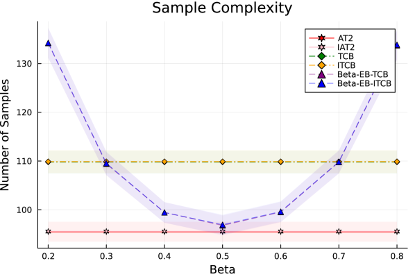
    Algorithm Avg. SC Std. Dev. AT2 95.47 1.02 IAT2 95.59 1.02 $0.5$-EB-TCB 96.78 1.02 $0.5$-EB-ITCB 96.94 1.02 TCB 109.8 1.17 ITCB 109.88 1.17

Figure 6: Sample complexity (SC) from Experiment 3, averaged over 4000 independent sample paths.

Experiment 4: In this experiment, we compare the run-time of (I)AT2 and (I)TCB algorithms on a 4 armed Gaussian bandit with means $\mu=[10,9.4,7,6.5]$ and unit variance, averaged over longer 100,000 simulations. Table 1 represents the average run-time of the two algorithms, We observe that TCB and ITCB take roughly two times more computational time compared to AT2 and IAT2, respectively.

Algorithm	Avg. Sample Complexity	Std. Dev.	Avg. Run Time (microsec.)	Run Time Std. Dev.
AT2	90.53	0.2	129.76	32.34
IAT2	90.63	0.2	310.76	55.88
TCB	96.55	0.21	501.22	82.60
ITCB	96.69	0.21	845.19	145.97

Table 1: Exp4: Runtime of (I)AT2 and (I)TCB on Gaussian bandit with $\mu=[10,9.4,7,6.5]$ and unit variances. Results reported are for $100,000$ independent runs of each algorithm.

7 Conclusion

We considered the best-arm identification problem under the popular top-2 framework. In the literature, top-2 framework involves sequentially identifying the empirical best arm and the most-likely challenger arm, and sampling the empirical best with probability $\beta$ and the other with the complimentary probability. However, optimal $\beta$ was not known. (Mukherjee and Tajer, 2023b) recently proposed a deterministic rule for deciding between the empirical best and the challenger arm. In this paper, we have provided a most natural first order optimality condition based rule to help decide between the two. We showed that our associated algorithm is asymptotically optimal, and empirically performs better than (Mukherjee and Tajer, 2023b) both in sample and computational complexity. Our another key contribution was to identify the underlying limiting ordinary differential equation based fluid dynamics that our algorithm tracks. This structure also helps prove convergence of the proposed algorithm.

Acknowledgements: We thank Arun Suggala and Karthikeyan Shanmugam from Google Research Bangalore for initial discussions on this project. They are not co-authors on their insistence. The second and the third author initiated this work while visiting Google Research in Bangalore.

Appendix

Appendix A Outline

Below we provide a brief outline of the topics presented in the appendices.

1. Algorithm (1) and (2) are, respectively, the pseudocodes of the AT2 and IAT2 algorithms introduced in Section 3.

2. Appendix B:  We define the single parameter exponential family (SPEF) of distributions, and prove several inequalities bounding the index function, anchor function, and the derivatives of the anchor function, which are crucial for our analysis.

3. Appendix C:  We provide the proofs omitted in Section 2.

4. Appendix D:  We introduce a framework using which we apply the implicit function theorem for proving several properties related to the fluid dynamics and the algorithm’s allocations.

5. Appendix E:  We provide the proofs of the results from Section 4, and also construct the fluid dynamics for the $\beta$-EB-TCB algorithm ([Jourdan et al., 2022]) in Appendix E.3.

6. Appendix F:  We prove Proposition 3.1, 5.1, and provide detailed proofs of all the results mentioned in Section 5.

7. Appendix G:  We provide the detailed proof of Theorem 3.1.

Input : Confidence parameter $\delta>0$, exploration parameter $\alpha\in(0,1)$

  for $N\geq 1$ do

     $\mathcal{V}_{N}\leftarrow\left\{a\in[K]~{}|~{}\widetilde{N}_{a}(N-1)<N^{\alpha}\right\}$

     if $\mathcal{V}_{N}\neq\emptyset$ then

        $A_{N}\leftarrow\text{argmin}_{a\in[K]}~{}{\widetilde{N}_{a}(N-1)}$

     else if $g(\mathbold{\widetilde{\mu}}(N-1),\mathbold{\widetilde{N}}(N-1))>0$ then

        $A_{N}\leftarrow\hat{i}_{N-1}$

     else

        $A_{N}\leftarrow\text{argmin}_{a\in[K]/\{\hat{i}_{N-1}\}}~{}{\mathcal{I}_{a}(N-1)}$

     end if

     Sample $X_{N}$ from $A_{N}$ and compute $\mathbold{\widetilde{\mu}}(N)$ and $\mathbold{\widetilde{N}}(N)$

     if $\min_{a\in[K]/\{\hat{i}_{N}\}}\mathcal{I}_{a}(N)>\beta(N,\delta)$ then

        Terminate and return $\hat{i}_{N}$

     end if

  end for

Algorithm 1 Anchored Top-Two (AT2) Algorithm

Input : Confidence parameter $\delta>0$, exploration parameter $\alpha\in(0,1)$

  for $N\geq 1$ do

     $\mathcal{V}_{N}\leftarrow\left\{a\in[K]~{}|~{}\widetilde{N}_{a}(N-1)<N^{\alpha}\right\}$

     if $\mathcal{V}_{N}\neq\emptyset$ then

        $A_{N}\leftarrow\text{argmin}_{a\in[K]}~{}{\widetilde{N}_{a}(N-1)}$

     else if $g(\mathbold{\widetilde{\mu}}(N-1),\mathbold{\widetilde{N}}(N-1))>0$ then

        $A_{N}\leftarrow\hat{i}_{N-1}$

     else

        $A_{N}\leftarrow\text{argmin}_{a\in[K]/\{\hat{i}_{N-1}\}}~{}{\mathcal{I}_{a}(N-1)+\log\widetilde{N}_{a}(N-1)}$

     end if

     Sample $X_{N}$ from $A_{N}$ and compute $\mathbold{\widetilde{\mu}}(N)$ and $\mathbold{\widetilde{N}}(N)$

     if $\min_{a\in[K]/\{\hat{i}_{N}\}}\mathcal{I}_{a}(N)>\beta(N,\delta)$ then

        Terminate and return $\hat{i}_{N}$

     end if

  end for

Algorithm 2 Improved Anchored Top-Two (IAT2) Algorithm

Appendix B Single parameter exponential family of distributions

We consider single parameter exponential family (SPEF) of distributions of the form

$$d\nu_{\theta}(x)=\exp(\theta x-b(\theta))d\rho(x)$$

where $\rho$ is a dominating measure which we assume to be degenerate, $\theta$ lies in the interior of set $\Theta$ defined below (denoted by $\Theta^{o}$):

$$\Theta=\left\{\theta~{}\Big{|}~{}\int_{\mathbb{R}}\exp(\theta x)d\rho(x)<\infty\right\},$$

and

$$b(\theta)=\log\left(\int_{\mathbb{R}}\exp(\theta x)d\rho(x)\right)$$

is the log-moment generating function of the measure $\rho(\cdot)$.

For $\theta,\widetilde{\theta}\in\Theta^{o}$, the KL-divergence between the measures $\nu_{\theta}$ and $\nu_{\widetilde{\theta}}$ is,

$$KL(\nu_{\theta},\nu_{\widetilde{\theta}})=(\theta-\widetilde{\theta})b^{\prime}(\theta)-b(\theta)+b(\widetilde{\theta}).$$

The mean under $\nu_{\theta}$ is given by $b^{\prime}(\theta)$. Let $\mathcal{S}$ be the image of the set $\Theta^{o}$ under the mapping $b^{\prime}(\cdot)$. Note that $\mathcal{S}$ is an open interval. Also, since, $b^{\prime\prime}(\cdot)>0$ in $\Theta^{o}$, $b^{\prime}(\cdot)$ is strictly increasing in $\Theta^{o}$, and is a bijection between $\Theta^{o}$ and $\mathcal{S}$. This implies we can parameterize the distributions in the SPEF using their means as well.

Let $\theta_{\mu}$ be the unique $\theta$ satisfying $b^{\prime}(\theta)=\mu$ for some $\mu\in\mathcal{S}$. Clearly, $\theta_{\mu}$ is a strictly increasing function of $\mu$. This follows since $b^{\prime}(\cdot)$ is strictly increasing in $\Theta^{o}$. Additionally, all the higher derivatives of $b(\cdot)$ exist in the set $\Theta^{o}$ (see Exercise 2.2.24 in [Dembo and Zeitouni, 2009]).

For $\mu,\widetilde{\mu}\in\mathcal{S}$ we define $d(\mu,\widetilde{\mu})$ as,

$$d(\mu,\widetilde{\mu})=KL(\nu_{\theta_{\mu}},\nu_{\theta_{\widetilde{\mu}}})=(\theta_{\mu}-\theta_{\widetilde{\mu}})\mu-b(\theta_{\mu})+b(\theta_{\widetilde{\mu}}).$$

We define $\mu_{\inf}\in\mathbb{R}\cup\{-\infty\}$ and $\mu_{\sup}\in\mathbb{R}\cup\{+\infty\}$, respectively, to be the infimum and supremum of the interval $\mathcal{S}$. Then, $\mathcal{S}=(\mu_{\inf},\mu_{\sup})$.

Definition B.1.

For $\mathbold{\mu}=(\mu_{1},\mu_{2},\ldots,\mu_{K})\in\mathcal{S}^{K}$, define $r_{\min}(\mathbold{\mu})=\min_{i\in[K]}\{\min\{\mu_{i}-\mu_{\inf},\mu_{\sup}-\mu_{i}\}\}$.

Since $\mathcal{S}$ is an open interval, $r_{\min}(\mathbold{\mu})$ is positive for every $\mathbold{\mu}\in\mathcal{S}^{K}$, and can be $\infty$ if both $\mu_{\inf}$ and $\mu_{\sup}$ are $\infty$.

Partial derivatives of $d(\mu,\widetilde{\mu})$:  For every pair $\mu,\widetilde{\mu}\in\mathcal{S}$, the partial derivatives of $d(\mu,\widetilde{\mu})$ with respect to the first argument is

$$d_{1}(\mu,\widetilde{\mu})\overset{\text{def.}}{=}\frac{\partial}{\partial\mu}d(\mu,\widetilde{\mu})=\theta_{\mu}-\theta_{\widetilde{\mu}},$$

and that with respect to the second argument is,

$$d_{2}(\mu,\widetilde{\mu})\overset{\text{def.}}{=}\frac{\partial}{\partial\widetilde{\mu}}d(\mu,\widetilde{\mu})=\frac{\widetilde{\mu}-\mu}{b^{\prime\prime}(\theta_{\widetilde{\mu}})}.$$

Enveloping the KL-divergence:  In the following discussion, we try to bound the KL-divergence $d(\mu,\widetilde{\mu})$ from both sides using the squared distance $|\mu-\widetilde{\mu}|^{2}$ after imposing some restrictions on the choice of $\mu,\widetilde{\mu}\in\mathcal{S}$. For an instance $\mathbold{\mu}\in\mathcal{S}^{K}$, we define the constants $\Delta_{\min}(\mathbold{\mu})$ and $\epsilon(\mathbold{\mu})$ as

$$\Delta_{\min}(\mathbold{\mu})=\min_{i\in[K]/\{1\}}(\mu_{1}-\mu_{i})\quad\text{and}\quad\epsilon(\mathbold{\mu})=\min\left\{\frac{\Delta_{\min}(\mathbold{\mu})}{4},\frac{r_{\min}(\mathbold{\mu})}{2}\right\}.$$

We further define

$$\mathcal{H}(\mathbold{\mu})=\bigcup_{i\in[K]/\{1\}}[\mu_{i}-\epsilon(\mathbold{\mu}),\mu_{1}+\epsilon(\mathbold{\mu})],\quad\sigma_{\max}(\mathbold{\mu})=\max_{\mu\in\mathcal{H}(\mathbold{\mu})}b^{\prime\prime}(\theta_{\mu})\quad\text{and}\quad\sigma_{\min}(\mathbold{\mu})=\min_{\mu\in\mathcal{H}(\mathbold{\mu})}b^{\prime\prime}(\theta_{\mu}).$$

Since $\mathcal{H}(\mathbold{\mu})\subset\mathcal{S}$, all distributions with mean in $\mathcal{H}(\mathbold{\mu})$ have positive variance. Note that $b^{\prime\prime}(\theta_{\mu})$ represents the variance of the distribution with mean $\mu$. As a result, since $\mathcal{H}(\mathbold{\mu})$ is a compact set, both $\sigma_{\max}(\mathbold{\mu})$ and $\sigma_{\min}(\mathbold{\mu})$ are positive constants.

Hence, $b(\cdot)$ is $\sigma_{\min}(\mathbold{\mu})$-strongly convex and $b^{\prime}(\cdot)$ is $\sigma_{\max}(\mathbold{\mu})$-Lipschitz on the set $(b^{\prime})^{-1}(\mathcal{H}(\mathbold{\mu}))$. Thus, using [Nesterov et al., 2018, Theorems 2.1.5 and 2.1.10], for every $\theta_{1},\theta_{2}\in(b^{\prime})^{-1}(\mathcal{H}(\mathbold{\mu}))$, we have

$$\frac{|b^{\prime}(\theta_{1})-b^{\prime}(\theta_{2})|^{2}}{2\sigma_{\max}(\mathbold{\mu})}\leq b(\theta_{2})-b(\theta_{1})-b^{\prime}(\theta_{1})\cdot(\theta_{2}-\theta_{1})=d(\nu_{\theta_{1}},\nu_{\theta_{2}})\leq\frac{|b^{\prime}(\theta_{1})-b^{\prime}(\theta_{2})|^{2}}{2\sigma_{\min}(\mathbold{\mu})},$$

and hence, for $\mu,\widetilde{\mu}\in\mathcal{H}(\mathbold{\mu})$,

$$\frac{|\mu-\widetilde{\mu}|^{2}}{2\sigma_{\max}(\mathbold{\mu})}\leq d(\mu,\widetilde{\mu})\leq\frac{|\mu-\widetilde{\mu}|^{2}}{2\sigma_{\min}(\mathbold{\mu})}.$$ (33)

Bounding the partial derivatives:  We now introduce bounds on the partial derivatives $d_{1}$ and $d_{2}$ introduced earlier. Consider $\mu,x,\widetilde{\mu}\in\mathcal{H}(\mathbold{\mu})$ such that $\mu>\widetilde{\mu}$, and $x\in[\widetilde{\mu},\mu]$. Recall

$$d_{1}(\mu,x)=\theta_{\mu}-\theta_{x}\quad\text{and}\quad d_{1}(\widetilde{\mu},x)=-(\theta_{x}-\theta_{\widetilde{\mu}}).$$

Since $\theta_{(\cdot)}=(b^{\prime})^{-1}(\cdot)$, we have,

$$\frac{\mu-x}{\sigma_{\max}(\mathbold{\mu})} \leq d_{1}(\mu,x)\leq\frac{\mu-x}{\sigma_{\min}(\mathbold{\mu})},\quad\text{and}\quad-\frac{x-\widetilde{\mu}}{\sigma_{\max}(\mathbold{\mu})}\geq d_{1}(\widetilde{\mu},x)\geq-\frac{x-\widetilde{\mu}}{\sigma_{\min}(\mathbold{\mu})}.$$ (34)

Similarly, since,

$$d_{2}(\mu,x)=-\frac{\mu-x}{b^{\prime\prime}(\theta_{x})}\quad\text{and}\quad d_{2}(\widetilde{\mu},x)=\frac{x-\widetilde{\mu}}{b^{\prime\prime}(\theta_{x})},$$

we have,

$$-\frac{\mu-x}{\sigma_{\max}(\mathbold{\mu})} \geq d_{2}(\mu,x)\geq-\frac{\mu-x}{\sigma_{\min}(\mathbold{\mu})},\quad\text{and}\quad\frac{x-\widetilde{\mu}}{\sigma_{\min}(\mathbold{\mu})}\leq d_{2}(\widetilde{\mu},x)\leq\frac{x-\widetilde{\mu}}{\sigma_{\min}(\mathbold{\mu})}.$$ (35)

B.1 Enveloping the anchor and index functions under noisy estimates of the rewards

For every arm $a\in[K]$, let $\widetilde{\mu}_{a}$ be an estimate of $\mu_{a}$ satisfying $|\widetilde{\mu}_{a}-\mu_{a}|\leq\epsilon(\mathbold{\mu})$ and $\mathbold{\widetilde{\mu}}=(\widetilde{\mu}_{a})_{a\in[K]}$. Since $\epsilon(\mathbold{\mu})\leq\frac{\Delta_{\min}(\mathbold{\mu})}{4}$, the empirically best arm with respect to the estimates $\mathbold{\widetilde{\mu}}$ is the first arm. Also let $N_{a}$ be the no. of times arm $a$ has been pulled and $\mathbold{N}=(N_{a})_{a\in[K]}$.

Enveloping the anchor function:  As we introduced in Section 3, the anchor function is,

$$g(\mathbold{\widetilde{\mu}},\mathbold{N})=\sum_{a\neq 1}\frac{d(\widetilde{\mu}_{1},\widetilde{x}_{1,a})}{d(\widetilde{\mu}_{a},\widetilde{x}_{1,a})}-1,$$

where $\widetilde{x}_{1,a}=\frac{N_{1}\widetilde{\mu}_{1}+N_{a}\widetilde{\mu}_{a}}{N_{1}+N_{a}}$. Note that $\widetilde{\mu}_{a},\widetilde{x}_{1,a}\in\mathcal{H}(\mathbold{\mu})$ for every $a\in[K]/\{1\}$. Therefore, using (33), we have,

$$\frac{\sigma_{\min}(\mathbold{\mu})}{\sigma_{\max}(\mathbold{\mu})}\sum_{a\neq 1}\frac{(\widetilde{\mu}_{1}-\widetilde{x}_{1,a})^{2}}{(\widetilde{x}_{1,a}-\widetilde{\mu}_{a})^{2}}-1~{} \leq~{}g(\mathbold{\widetilde{\mu}},\mathbold{N})~{}\leq~{}\frac{\sigma_{\max}(\mathbold{\mu})}{\sigma_{\min}(\mathbold{\mu})}\sum_{a\neq 1}\frac{(\widetilde{\mu}_{1}-\widetilde{x}_{1,a})^{2}}{(\widetilde{x}_{1,a}-\widetilde{\mu}_{a})^{2}}-1,$$

Putting $\widetilde{x}_{1,a}=\frac{N_{1}\widetilde{\mu}_{1}+N_{a}\widetilde{\mu}_{a}}{N_{1}+N_{a}}$, we obtain,

$$\frac{\sigma_{\min}(\mathbold{\mu})}{\sigma_{\max}(\mathbold{\mu})}\sum_{a\neq 1}\frac{N_{a}^{2}}{N_{1}^{2}}-1~{} \leq~{}g(\mathbold{\widetilde{\mu}},\mathbold{N})~{}\leq~{}\frac{\sigma_{\max}(\mathbold{\mu})}{\sigma_{\min}(\mathbold{\mu})}\sum_{a\neq 1}\frac{N_{a}^{2}}{N_{1}^{2}}-1,$$ (36)

Now $\widetilde{\mu}_{1}-\widetilde{x}_{1,a}=\frac{N_{a}}{N_{1}+N_{a}}(\widetilde{\mu}_{1}-\widetilde{\mu}_{a})$ and $\widetilde{x}_{1,a}-\widetilde{\mu}_{a}=\frac{N_{1}}{N_{1}+N_{a}}(\widetilde{\mu}_{1}-\widetilde{\mu}_{a})$. Using these, we can say,

$$g(\mathbold{\widetilde{\mu}},\mathbold{N})~{} =~{}\Theta\left(\sum_{a\neq 1}\frac{N^{2}_{a}}{N^{2}_{1}}\right)-1,$$ (37)

whenever $|\widetilde{\mu}_{a}-\mu_{a}|\leq\epsilon(\mathbold{\mu})$ for all $a\in[K]$. The constants hidden in the $\Theta(\cdot)$ depends only on $\mathbold{\mu}$ and obviously the choice of the SPEF family.

Enveloping the index:  Following the definition of empirical index $\mathcal{I}_{a}(\cdot)$ in Section 3, we define the index of any alternative arm $a\in[K]/\{1\}$ with respect to the estimates $\mathbold{\widetilde{\mu}}=(\widetilde{\mu}_{a}:a\in[K])$ and allocation $\mathbold{N}=(N_{a}:a\in[K])$ is,

$$\mathcal{W}_{a}(\mathbold{\widetilde{\mu}},\mathbold{N})~{}=~{}N_{1}d(\widetilde{\mu}_{1},\widetilde{x}_{1,a})+N_{a}d(\widetilde{\mu}_{a},\widetilde{x}_{1,a}).$$

Observe that, the empirical index $\mathcal{I}_{a}(N)$ and index $I_{a}(N)$ introduced in Section 3 are, respectively, equivalent to the quantities $\mathcal{W}_{a}(\mathbold{\widetilde{\mu}}(N),\mathbold{\widetilde{N}}(N))$, and $\mathcal{W}_{a}(\mathbold{\mu},\mathbold{\widetilde{N}}(N))$, where $\mathbold{\widetilde{\mu}}(N)$ is the empirical estimate and $\mathbold{\widetilde{N}}(N)$ is the algorithm’s allocation at iteration $N$.

Using (33) we have,

$$\frac{1}{2\sigma_{\min}(\mathbold{\mu})}(N_{1}(\widetilde{\mu}_{1}-\widetilde{x}_{1,a})^{2}+N_{a}(\widetilde{x}_{1,a}-\widetilde{\mu}_{a})^{2})~{} \leq~{}\mathcal{W}_{a}(\mathbold{\widetilde{\mu}},\mathbold{N})~{}\leq~{}\frac{1}{2\sigma_{\min}(\mathbold{\mu})}(N_{1}(\widetilde{\mu}_{1}-\widetilde{x}_{1,a})^{2}+N_{a}(\widetilde{x}_{1,a}-\widetilde{\mu}_{a})^{2}).$$

Putting $\widetilde{x}_{1,a}=\frac{N_{1}\widetilde{\mu}_{1}+N_{a}\widetilde{\mu}_{a}}{N_{1}+N_{a}}$, we get,

$$\frac{(\widetilde{\mu}_{1}-\widetilde{\mu}_{a})^{2}}{2\sigma_{\max}(\mathbold{\mu})}\frac{N_{1}N_{a}}{N_{1}+N_{a}}~{} \leq~{}\mathcal{W}_{a}(\mathbold{\widetilde{\mu}},\mathbold{N})~{}\leq~{}\frac{(\widetilde{\mu}_{1}-\widetilde{\mu}_{a})^{2}}{2\sigma_{\min}(\mathbold{\mu})}\frac{N_{1}N_{a}}{N_{1}+N_{a}},~{}\text{which implies,}$$

$$\frac{(\mu_{1}-\mu_{a}-2\epsilon(\mathbold{\mu}))^{2}}{2\sigma_{\max}(\mathbold{\mu})}\frac{N_{1}N_{a}}{N_{1}+N_{a}}~{} \leq~{}\mathcal{W}_{a}(\mathbold{\widetilde{\mu}},\mathbold{N})~{}\leq~{}\frac{(\mu_{1}-\mu_{a}+2\epsilon(\mathbold{\mu}))^{2}}{2\sigma_{\min}(\mathbold{\mu})}\frac{N_{1}N_{a}}{N_{1}+N_{a}}.$$

We define $\Delta_{\max}(\mathbold{\mu})=\max_{a\in[K]/\{1\}}\Delta_{a}$. Since $\epsilon(\mathbold{\mu})\leq\frac{1}{4}\delta_{\min}(\mathbold{\mu})$, we have,

$$\frac{\Delta_{\min}(\mathbold{\mu})^{2}}{8\sigma_{\max}(\mathbold{\mu})}\frac{N_{1}N_{a}}{N_{1}+N_{a}}~{} \leq~{}\mathcal{W}_{a}(\mathbold{\widetilde{\mu}},\mathbold{N})~{}\leq~{}\frac{(\Delta_{\max}(\mathbold{\mu})+2\epsilon(\mathbold{\mu}))^{2}}{2\sigma_{\min}(\mathbold{\mu})}\frac{N_{1}N_{a}}{N_{1}+N_{a}}.$$ (38)

Using the same notation, as we used in (37), we have,

$$\mathcal{W}_{a}(\mathbold{\widetilde{\mu}},\mathbold{N})~{} =~{}\Theta\left(\frac{N_{1}N_{a}}{N_{1}+N_{a}}\right)$$ (39)

for every arm $a\in[K]/\{1\}$.

Enveloping the partial derivatives of anchor function with respect to $\mathbold{N}$:  While analyzing the AT2 and IAT2 algorithms, we need to show that the anchor function converges to zero at a uniform rate as no. of iteration goes to infinity. During this step, we need to bound the partial derivatives of the anchor function $g(\mathbold{\mu},\mathbold{N})$ with respect to $\mathbold{N}$. Below we evaluate the partial derivatives of $g(\mathbold{\mu},\mathbold{N})$ with respect to $N_{a}$ for different arms $a\in[K]$.

$$\frac{\partial g}{\partial N_{1}}(\mathbold{\mu},\mathbold{N}) =-\sum_{a\neq 1}f(\mathbold{\mu},a,\mathbold{N})\frac{N_{a}\Delta_{a}}{(N_{1}+N_{a})^{2}},~{}\text{and}$$

$$\forall a\neq 1,~{}~{}\frac{\partial g}{\partial N_{a}}(\mathbold{\mu},\mathbold{N}) =f(\mathbold{\mu},a,\mathbold{N})\frac{N_{1}\Delta_{a}}{(N_{1}+N_{a})^{2}},~{}~{}\text{where}$$ (40)

$$\Delta_{a}=\mu_{1}-\mu_{a}~{} \text{and}~{}f(\mathbold{\mu},a,\mathbold{N})=-\frac{\partial}{\partial x}\left(\frac{d(\mu_{1},x)}{d(\mu_{a},x)}\right)\Big{|}_{x=x_{1,a}}=-\frac{d_{2}(\mu_{1},x_{1,a})}{d(\mu_{a},x_{1,a})}+\frac{d(\mu_{1},x_{1,a})d_{2}(\mu_{a},x_{1,a})}{(d(\mu_{a},x_{1,a}))^{2}}.$$

Using (35), and (33), we have,

$$-d_{2}(\mu_{1},x_{1,a})~{} =~{}\Theta(\mu_{1}-x_{1,a}),\quad d_{2}(\mu_{a},x_{1,a})~{}=~{}\Theta(x_{1,a}-\mu_{a}),$$

$$d(\mu_{1},x_{1,a})~{} =~{}\Theta((\mu_{1}-x_{1,a})^{2}),\quad\text{and}\quad d(\mu_{a},x_{1,a})~{}=~{}\Theta((x_{1,a}-\mu_{a})^{2}),$$

where the constants hidden in $\Theta(\cdot)$ depend only on $\mathbold{\mu}$ and are independent of the sample path. Therefore,

$$f(\mathbold{\mu},a,\mathbold{N}) =\Theta\left(\frac{\mu_{1}-x_{1,a}}{(x_{1,a}-\mu_{a})^{2}}+\frac{(\mu_{1}-x_{1,a})^{2}}{(x_{1,a}-\mu_{a})^{3}}\right)$$

$$=\Theta\left(\frac{N_{a}}{N_{1}}\left(1+\frac{N_{a}}{N_{1}}\right)^{2}\right).$$ (41)

As a consequence, we have,

$$\frac{\partial g}{\partial N_{1}}(\mathbold{\mu},\mathbold{N}) =-\Theta\left(\sum_{a\in[K]/\{1\}}\frac{N_{a}^{2}}{N_{1}^{3}}\right),~{}~{}\text{and}$$

$$\forall a\neq 1,~{}~{}\frac{\partial g}{\partial N_{a}}(\mathbold{\mu},\mathbold{N}) =\Theta\left(\frac{N_{a}}{N_{1}^{2}}\right).$$ (42)

Appendix C Proofs from Section 2

Proof of Theorem 2.1:

We restate the theorem with some more detail. Some notation is needed for that. Recall that $B$ is a subset of $\{2,\ldots,K\}$, each $\nu_{i}\in{\cal S}$ and $\nu_{1}>\max_{i\geq 2}\nu_{i}$, $\overline{B}=B\cup\{1\}$. If $\overline{B}^{c}\neq\emptyset$ then let $(N_{a}\in\mathbb{R}_{\geq 0}:a\in\overline{B}^{c})$ be the no. of samples allocated to arms in $\overline{B}^{c}$. We define $N_{1,1}$ as zero when $\sum_{a\in\overline{B}^{c}}N_{a}=0$ or $\overline{B}^{c}=\emptyset$. Otherwise, we take $N_{1,1}$ to be the unique $N_{1}>0$ that solves,

$$\sum_{a\in\overline{B}^{c}}\frac{d(\nu_{1},x_{1,a})}{d(\nu_{a},x_{1,a})}=1,$$ (43)

where $x_{1,a}=\frac{\nu_{1}N_{1}+\nu_{a}N_{a}}{N_{1}+N_{a}}$. Note that if $\overline{B}^{c}\neq\emptyset$ and $\sum_{a\in\overline{B}^{c}}N_{a}>0$, there exists an $a\in\overline{B}^{c}$ with $N_{a}>0$. As a result, the LHS of (43) decreases from $\infty$ to $0$ as $N_{1}$ increases from $0$ to $\infty$. This implies the existence of a unique $N_{1}>0$ solving (43).

Set $N_{1,2}:=\max_{a\in B}I_{a}{d(\nu_{1},\nu_{a})^{-1}}$.

Theorem C.1.

There exists a unique solution $N_{1}^{\star}\geq 0$ and $(N^{\star}_{a}\geq 0:a\in B)$ satisfying

$$\sum_{a\neq 1}\frac{d(\nu_{1},{x}^{\star}_{1,a})}{d(\nu_{a},{x}^{\star}_{1,a})}-1=0\quad\mbox{ where }\quad x^{\star}_{1,a}=\frac{\nu_{1}N^{\star}_{1}+\nu_{a}N^{\star}_{a}}{N^{\star}_{1}+N^{\star}_{a}},$$ (44)

$$\mbox{ and }\quad N^{\star}_{1}d(\nu_{1},x^{\star}_{1,a})+N^{\star}_{a}d(\nu_{a},x^{\star}_{1,a})=I_{a}\quad\forall a\in B.$$ (45)

Further, $N^{\star}_{1}\geq\max(N_{1,1},N_{1,2})$ and each $N_{a}^{\star}\geq\frac{I_{a}}{d(\nu_{a},\nu_{1})}$. Furthermore, The optimal solution to $\mathbf{O}$ is uniquely characterized by the solution above with $B=\{2,\ldots,K\}$ and each $I_{a}=\log(1/(2.4\delta))$ and constraints (1) tight, that is, indexes $(I_{a}(N^{\star}):a\neq 1)$ equal to each other and RHS. Further, $N_{1}^{\star}\geq\max_{a\in[K]\setminus{1}}\frac{\log(1/(2.4\delta)}{d(\nu_{1},\nu_{a})}$ and each $N_{a}^{\star}\geq\frac{\log(1/(2.4\delta)}{d(\nu_{a},\nu_{1})}$.

Proof: First observe that every solution $N_{1}^{\star}$ and $(N_{a}^{\star}:a\in B)$ to the system (44) and (45) must satisfy $N_{1}\geq\max\{N_{1,1},N_{1,2}\}$ and $N_{a}^{\star}\geq\frac{I_{a}}{d(\nu_{a},\nu_{1})}$, for every $a\in B$.

If $\overline{B}^{c}\neq\emptyset$, (44) implies,

$$\sum_{a\in\overline{B}^{c}}\frac{d(\nu_{1},x_{1,a})}{d(\nu_{a},x_{1,a})}~{}\leq~{}\sum_{a\in[K]/\{1\}}\frac{d(\nu_{1},x_{1,a})}{d(\nu_{a},x_{1,a})}~{}=~{}1.$$

If $\sum_{a\in\overline{B}^{c}}N_{a}=0$, then $N_{1}\geq 0=N_{1,1}$. Otherwise, we can find an $a\in\overline{B}^{c}$ with $N_{a}>0$, making $\sum_{a\in\overline{B}^{c}}\frac{d(\nu_{1},x_{1,a})}{d(\nu_{a},x_{1,a})}$ strictly decreasing in $N_{1}$. As a result, by the definition of $N_{1,1}$ we have $N_{1}^{\star}\geq N_{1,1}$.

Now, for every $a\in B$, we have

$$I_{a}~{}=~{}N_{1}^{\star}d(\nu_{1},x_{1,a})+N_{a}^{\star}d(\nu_{a},x_{1,a})~{}=~{}\min_{x\in[\nu_{a},\nu_{1}]}\{N_{1}^{\star}d(\nu_{1},x)+N_{a}^{\star}d(\nu_{a},x)\}.$$

Note that RHS of the above inequality is upper bounded by $\min\{N_{1}^{\star}d(\nu_{1},\nu_{a}),N_{a}^{\star}d(\nu_{a},\nu_{1})\}$. As a result, for every $a\in B$, $N_{a}^{\star}\geq\frac{I_{a}}{d(\nu_{a},\nu_{1})}$, and $N_{1}^{\star}\geq\frac{I_{a}}{d(\mu_{1},\mu_{a})}$. This further implies, $N_{1}^{\star}\geq\max_{a\in B}\frac{I_{a}}{d(\nu_{1},\nu_{a})}=N_{1,2}$.

Now we prove existence of a unique $N_{1}^{\star}$ and $(N_{a}^{\star}:a\in B)$. For every $N_{1}\geq N_{1,2}$ and $a\in B$, as $N_{a}$ increases from $0$ to $\infty$, $N_{1}d(\nu_{1},x_{1,a})+N_{a}d(\nu_{a},x_{1,a})$ increases monotonically from $0$ to $N_{1}d(\nu_{1},\nu_{a})$. Note that $N_{1}d(\nu_{1},\nu_{a})\geq N_{1,2}d(\nu_{1},\nu_{a})\geq I_{a}$ (by the definition of $N_{1,2}$). As a result, we can find a unique $N_{a}$ for which $N_{1}d(\nu_{1},x_{1,a})+N_{a}d(\nu_{a},x_{1,a})=I_{a}$. For every $a\in B$, we call that unique $N_{a}$ as $N_{a}(N_{1})$. Observe that, since $I_{a}>0$, $N_{a}(N_{1})$ is strictly decreasing in $N_{1}$, and if $I_{a}=0$, then $N_{a}(N_{1})=0$. Also, if $a=\text{argmax}_{b\in B}~{}{\frac{I_{b}}{d(\nu_{1},\nu_{b})}}$, then $N_{a}(N_{1,2})=\infty$ and $\lim_{N_{1}\to\infty}N_{a}(N_{1})=\frac{I_{a}}{d(\nu_{a},\nu_{1})}$.

We now consider the allocation where every arm $a\in B$ has $N_{a}(N_{1})$ samples, and consider the function,

$$h(N_{1})~{}=~{}\sum_{a\in[K]/\{1\}}\frac{d(\nu_{1},x_{1,a})}{d(\nu_{a},x_{1,a})}.$$

Observe that, for all $a\in B$, $\frac{d(\nu_{1},x_{1,a})}{d(\nu_{a},x_{1,a})}$ is strictly decreasing for $N_{1}\geq N_{1,2}$. Also if $\overline{B}^{c}$ is non-empty, then every term $\frac{d(\nu_{1},x_{1,a})}{d(\nu_{a},x_{1,a})}$ with $N_{a}>0$ is strictly decreasing in $N_{1}$. As a result, the overall function $N_{1}\to h(N_{1})$ is strictly decreasing.

Moreover, as $N_{1}$ increases to $\infty$, $N_{a}(N_{1})$ converges to $\frac{I_{a}}{d(\nu_{a},\nu_{1})}$, for every $a\in B$. Hence, $h(N_{1})$ decreases to $0$ as $N_{1}\to\infty$. Therefore, if we can show that $h(\max\{N_{1,1},N_{2,1}\})\geq 1$, then we can find a unique $N_{1}^{\star}\geq\max\{N_{1,1},N_{1,2}\}$ at which $h(N_{1}^{\star})=1$, and can take $N_{a}^{\star}=N_{a}(N_{1}^{\star})$ for every $a\in B$. Following this, to prove uniqueness, it is sufficient to show $h(\max\{N_{1,1},N_{1,2}\})\geq 1$.

If $N_{1,2}\geq N_{1,1}$, then some $a\in B$ has $N_{a}(N_{1,2})=\infty$. As a result, we have $h(N_{1,2})=\infty\geq 1$. Otherwise, if $N_{1,1}\geq N_{1,2}>0$, then by definition of $N_{1,1}$, we have

$$h(N_{1,1})~{}\geq~{}\sum_{a\in\overline{B}^{c}}\frac{d(\nu_{1},x_{1,a})}{d(\nu_{a},x_{1,a})}=1.$$

Hence we finish proving the first part of Theorem C.1.

To see the necessity of the stated optimality conditions for ${\bf O}$ observe that we cannot have $N_{1}^{\star}=0$ or $N_{a}^{\star}=0$ as that implies that the index $W_{a}(N_{1}^{\star},N_{a}^{\star})$ is zero. Further, if $W_{a}(N_{1}^{\star},N_{a}^{\star})>1$, the objective improves by reducing $N_{a}^{\star}$. Thus the constraints (1) must be tight. To see the tightness of (1) again note that the derivative of $W_{a}(N_{1},N_{a})$ with respect to $N_{1}$ and $N_{a}$, respectively, equals $d(\mu_{1},x_{1,a})$ and $d(\mu_{a},x_{1,a})$.

Now, perturbing $N_{1}$ by a tiny $\epsilon$ and adjusting each $N_{a}$ by $\frac{d(\mu_{1},x_{1,a})}{d(\mu_{a},x_{1,a})}\epsilon$ maintains the value of $W_{a}(N_{1}^{\star},N_{a}^{\star})$. Thus, at optimal $\mathbold{N}^{\star}$, necessity of tightness of inequalities in (1) follows. This condition can also be seen through the Lagrangian (see [Agrawal et al., 2023]).

The fact that these three criteria uniquely specify the optimal solution follows from our analysis above. Since the convex problem ${\bf O}$ has a solution, the uniqueness of the solution above satisfying the necessary conditions implies that this uniquely solves ${\bf O}$. ∎

Appendix D Framework for applying the Implicit function theorem (IFT)

In this appendix we explain a general framework using which we later apply the Implicit function theorem for the following purposes:

1. Constructing the fluid dynamics for the AT2 and $\beta$-EB-TCB algorithms in Appendix E.1.

2. Proving convergence of the algorithm’s allocations to the optimal proportions in Appendix F.2.2.

We introduce the variables:  $\mathbold{N}=(N_{a}\in\mathbb{R}_{\geq 0}:a\in[K])$,  $I\in\mathbb{R}$,  $\mathbold{\eta}=(\eta_{a}\in\mathbb{R}:a\in[K])$,  and  $N\geq 0$. After fixing some instance $\mathbold{\mu}\in\mathcal{S}^{K}$ ($\mathcal{S}$ is defined in Appendix B), we define the following functions:

$$\Phi_{1}(\mathbold{N},\mathbold{\eta})~{} =~{}\sum_{a\in[K]/\{1\}}\frac{d(\mu_{1},x_{1,a}(N_{1},N_{a}))}{d(\mu_{a},x_{1,a}(N_{1},N_{a}))}-1-\eta_{1},$$

$$\text{for}~{}a\in[K]/\{1\},\quad\Phi_{a}(\mathbold{N},I,\mathbold{\eta})~{} =~{}N_{1}d(\mu_{1},x_{1,a}(N_{1},N_{a}))+N_{a}d(\mu_{a},x_{1,a}(N_{1},N_{a}))-I-\eta_{a},\quad\text{and}$$

$$\Phi_{K+1}(\mathbold{N},N)~{} =~{}\sum_{a\in[K]}N_{a}-N,$$

where

$$x_{1,a}(N_{1},N_{a})=\frac{N_{1}\mu_{1}+N_{a}\mu_{a}}{N_{1}+N_{a}}.$$

For every non-empty subset $B\subseteq[K]/\{1\}$, we define the vector valued functions,

$$\mathbold{\Phi}_{B}(\mathbold{N},I,\mathbold{\eta},N)~{} =~{}\left[~{}\Phi_{1}(\mathbold{N},\mathbold{\eta}),\quad(\Phi_{a}(\mathbold{N},I,\mathbold{\eta}))_{a\in B},\quad\Phi_{K+1}(\mathbold{N},N)~{}\right],\quad\text{and}$$

$$\mathbold{\widetilde{\Phi}}_{B}(\mathbold{N},I,\mathbold{\eta})~{} =~{}\left[~{}\Phi_{1}(\mathbold{N},\mathbold{\eta}),\quad(\Phi_{a}(\mathbold{N},I,\mathbold{\eta}))_{a\in B}~{}\right].$$

We denote $\mathbold{\Phi}_{[K]/\{1\}}(\cdot)$ just using $\mathbold{\Phi}(\cdot)$.

In the definitions of $\mathbold{\Phi}_{B}(\cdot)$ and $\mathbold{\widetilde{\Phi}}_{B}(\cdot)$, without loss of generality, we assume that, the functions $\Phi_{a}(\cdot)$ in the tuple $(\Phi_{a}(\cdot))_{a\in B}$ are enumerated in the increasing order of $a\in B$, i.e., if we have $B=\{a_{1},a_{2},\ldots,a_{|B|}\}$ with $1<a_{1}<a_{2}<\ldots<a_{|B|}$, then,

$$\mathbold{\Phi}_{B}~{} =~{}\left[~{}\Phi_{1},\quad\Phi_{a_{1}},\quad,\Phi_{a_{2}},\quad\Phi_{a_{3}},\quad\ldots\quad\Phi_{a_{|B|}},\quad\Phi_{K+1}~{}\right],\quad\text{and}$$

$$\widetilde{\mathbold{\Phi}}_{B}~{} =~{}\left[~{}\Phi_{1},\quad\Phi_{a_{1}},\quad,\Phi_{a_{2}},\quad\Phi_{a_{3}},\quad\ldots\quad\Phi_{a_{|B|}}~{}\right].$$

Before stating the main result of this section in Lemma D.1, we define some notation that are essential for the lemma statement. For any $A\subseteq[K]$, we use the notation $\mathbold{N}_{A}$ to denote the tuple of variables $(N_{a}:a\in A)$. For some vector valued function $\mathbold{G}$ depending on $\mathbold{N}$, denote the Jacobian of $G(\cdot)$ with respect to the tuple of variables $\mathbold{N}_{A}$ using $\frac{\partial\mathbold{G}}{\partial\mathbold{N}_{A}}$.

For any non-empty $B\subseteq[K]/\{1\}$, we define $\overline{B}=B\cup\{1\}$. For every $k\geq 1$, $\mathbf{0}_{k}$ and $\mathbf{1}_{k}$, respectively, refers to a $k$-dimensional vector with entries $0$ and $1$. We define $\mathcal{Z}_{B}$ to be the set of tuples $(\mathbold{N},I,\mathbf{0}_{K},N)$ with  $\mathbold{N}\in\mathbb{R}_{\geq 0}^{K}$,  $I\in\mathbb{R}$,  and  $N\in\mathbb{R}_{>0}$,  which satisfy

$$\mathbold{\Phi}_{B}(\mathbold{N},I,\mathbf{0}_{K},N)~{}=~{}\mathbf{0}_{|B|+2}.$$

Lemma D.1 (Invertibility of the Jacobian).

For all non-empty subset $B\subseteq[K]/\{1\}$, the following statements hold true at every tuple $(\mathbold{N},I,\mathbf{0}_{K},N)$ in the set $\mathcal{Z}_{B}$,

1. The Jacobian $\frac{\partial\mathbold{\widetilde{\Phi}}_{B}}{\partial\mathbold{N}_{\overline{B}}}$ is invertible at $(\mathbold{N},I,\mathbf{0}_{K})$.

2. We have

   $$\mathbf{1}_{|B|+1}^{T}\left(\frac{\partial\mathbold{\widetilde{\Phi}}_{B}}{\partial\mathbold{N}_{\overline{B}}}\right)^{-1}\frac{\partial\mathbold{\widetilde{\Phi}}_{B}}{\partial I}\leq-\sum_{a\in B}\frac{1}{d(\mu_{a},\mu_{1})},$$

   at $(\mathbold{N},I,\mathbf{0}_{K})$.

3. The Jacobian $\frac{\partial\mathbold{\Phi}_{B}}{\partial(\mathbold{N}_{\overline{B}},I)}$ defined as,

   $$\frac{\partial\mathbold{\Phi}_{B}}{\partial(\mathbold{N}_{\overline{B}},I)}~{} =~{}\left[\begin{array}[]{c|c}&\\ \frac{\partial\mathbold{\widetilde{\Phi}}_{B}}{\partial\mathbold{N}_{\overline{B}}}&\frac{\partial\mathbold{\widetilde{\Phi}}_{B}}{\partial I}\\ &\\ \hline\cr\\ \frac{\partial\Phi_{K+1}}{\partial\mathbold{N}_{\overline{B}}}&\frac{\partial\Phi_{K+1}}{\partial I}\\ &\end{array}\right]$$

   is invertible at $(\mathbold{N},I,\mathbf{0}_{K},N)$.

Proof.

Statement 1:  The Jacobian $\frac{\partial\mathbold{\widetilde{\Phi}}_{B}}{\partial\mathbold{N}_{\overline{B}}}$ is equivalent to,

$$\frac{\partial\mathbold{\widetilde{\Phi}}_{B}}{\partial\mathbold{N}_{\overline{B}}} =\begin{bmatrix}\frac{\partial\Phi_{1}}{\partial N_{1}}&\frac{\partial\Phi_{1}}{\partial N_{a_{1}}}&\frac{\partial\Phi_{1}}{\partial N_{a_{2}}}&\ldots&\frac{\partial\Phi_{1}}{\partial N_{a_{|B|}}}\\ \frac{\partial\Phi_{a_{1}}}{\partial N_{1}}&\frac{\partial\Phi_{a_{1}}}{\partial N_{a_{1}}}&\frac{\partial\Phi_{a_{1}}}{\partial N_{a_{2}}}&\ldots&\frac{\partial\Phi_{a_{1}}}{\partial N_{a_{|B|}}}\\ \vdots&\vdots&\vdots&\ldots&\vdots\\ \frac{\partial\Phi_{a_{|B|}}}{\partial N_{1}}&\frac{\partial\Phi_{a_{|B|}}}{\partial N_{a_{1}}}&\frac{\partial\Phi_{a_{|B|}}}{\partial N_{a_{2}}}&\ldots&\frac{\partial\Phi_{a_{|B|}}}{\partial N_{a_{|B|}}}\end{bmatrix}.$$ (46)

Now we observe the following properties about the sign of the entries of the above Jacobian matrix,

• We have $N>0$ and $\Phi_{1}(\mathbold{N},\mathbf{0}_{K})=0$. This implies $N_{1}>0$ and $\max_{a\in[K]/\{1\}}N_{a}>0$. As a result, using (B.1), we have $\frac{\partial\Phi_{1}}{\partial N_{1}}<0$ and $\frac{\partial\Phi_{1}}{\partial N_{a_{i}}}\geq 0$ for every $i\in\{1,2,\ldots,|B|\}$.

• For $i\in\{2,\ldots,|B|+1\}$, in the $i$-th row, the only non-zero entries can be the first and the $i$-th entry. The first entry is $\frac{\partial\Phi_{a_{i}}}{\partial N_{1}}=d(\mu_{1},x_{1,a_{i}}(N_{1},N_{a_{i}}))\geq 0$. The $i$-th entry is $\frac{\partial\Phi_{a_{i}}}{\partial N_{a_{i}}}=d(\mu_{a_{i}},x_{1,a_{i}}(N_{1},N_{a_{i}}))$. Since we have $N_{1}>0$, using (33), we have $d(\mu_{a_{i}},x_{1,a_{i}}(N_{1},N_{a_{i}}))>0$, making the $i$-th entry positive.

Therefore, considering only the sign of the elements, the matrix in (46) is of the form,

$$\begin{bmatrix}--&+&+&+&\ldots&+\\ +&++&0&0&\ldots&0\\ +&0&++&0&\ldots&0\\ +&0&0&++&\ldots&0\\ \vdots&\vdots&\vdots&\vdots&\ldots&\vdots\\ +&0&0&0&\ldots&++\end{bmatrix},$$ (47)

where the symbols $++,~{}--$ and $+$ implies that the corresponding entries are positive, negative and non-negative.

We now argue that a matrix of the above structure has a rank $|B|+1$. To see that, by subtracting some appropriate constant times the $i$-th column from the first column, we can make the entries in position $i\in\{2,3,\ldots,|B|+1\}$ in the first column zero. As a result of these transformations, since we are subtracting non-negative quantities from the first entry of the first column, that entry remains negative. The matrix we obtain after this sequence of transformations has a structure,

$$\begin{bmatrix}--&+&+&+&\ldots&+\\ 0&++&0&0&\ldots&0\\ 0&0&++&0&\ldots&0\\ 0&0&0&++&\ldots&0\\ \vdots&\vdots&\vdots&\vdots&\ldots&\vdots\\ 0&0&0&0&\ldots&++\end{bmatrix}.$$ (48)

Clearly a matrix of the above structure has a rank $|B|+1$ and therefore invertible.

Statement 2:  Using statement 1 of Lemma D.1, if we take $\mathbold{v}=\left(\frac{\partial\mathbold{\widetilde{\Phi}}_{B}}{\partial\mathbold{N}_{\overline{B}}}\right)^{-1}\frac{\partial\mathbold{\widetilde{\Phi}}_{B}}{\partial I}$, then we have,

$$\frac{\partial\mathbold{\widetilde{\Phi}}_{B}}{\partial\mathbold{N}_{\overline{B}}}\mathbold{v}~{}=~{}\frac{\partial\mathbold{\widetilde{\Phi}}_{B}}{\partial I}.$$

Note that, the RHS of the above linear system i.e. $\frac{\partial\mathbold{\widetilde{\Phi}}_{B}}{\partial I}$ is a $|B|+1$ dimensional vector with zero in its first entry and $-1$ in every other entry. Using (48), $\mathbold{v}=[v_{1},v_{2},v_{3},\ldots,v_{|B|+1}]^{T}$ satisfies a linear system with coefficients having the following signs,

$$(--)v_{1}+(+)v_{2}+(+)v_{3}+(+)v_{4}+\ldots+(+)v_{|B|+1}~{} =~{}0,\quad\text{and}$$

$$\text{for}~{}~{}i\in\{2,\ldots,|B|+1\},\quad(+)v_{1}+(++)v_{i}~{} =~{}(--),$$

where $++$, $--$ and $+$ represents quantities which are positive, negative and non-negative.

For every $i\in\{2,\ldots,|B|+1\}$, we can eliminate $v_{i}$ from the first equation by subtracting some positive constant times the $i$-th equation from it. After eliminating $v_{2},v_{3},\ldots,v_{|B|+1}$ from the first equation following the mentioned procedure, we will be left with an equation of the form $(--)v_{1}=(+)$, implying $v_{1}\leq 0$.

Now the $i$-th equation of the system, for $i\in\{2,\ldots,|B|+1\}$ is,

$$\frac{\partial\Phi_{a_{i-1}}}{\partial N_{1}}v_{1}+\frac{\partial\Phi_{a_{i-1}}}{\partial N_{a_{i-1}}}v_{i}~{} =~{}-1.$$ (49)

We know that, $\frac{\partial\Phi_{a_{i-1}}}{\partial N_{1}}=d(\mu_{1},x_{1,{a_{i-1}}})$ and $\frac{\partial\Phi_{a_{i-1}}}{\partial N_{a_{i-1}}}=d(\mu_{a_{i-1}},x_{1,{a_{i-1}}})$, where $x_{1,a}=\frac{N_{1}\mu_{1}+N_{a}\mu_{a}}{N_{1}+N_{a}}$ for every $a\in[K]/\{1\}$.

Now putting the derivatives in (49), we have

$$d(\mu_{1},x_{1,a_{i-1}})v_{1}+d(\mu_{a_{i-1}},x_{1,a_{i-1}})v_{i}~{}=~{}-1,$$

which implies,

$$v_{i}~{}=~{}-\frac{1}{d(\mu_{a_{i-1}},x_{1,a_{i-1}})}-\frac{d(\mu_{1},x_{1,a_{i-1}})}{d(\mu_{a_{i-1}},x_{1,a_{i-1}})}v_{1},$$

for every $i\in\{2,\ldots,|B|+1\}$.

Now adding both sides for $i\in\{2,3,\ldots,|B|+1\}$, we get,

$$\sum_{i=2}^{|B|+1}v_{i}~{} =~{}-\sum_{i=2}^{|B|+1}\frac{1}{d(\mu_{a_{i-1}},x_{1,a_{i-1}})}-v_{1}\sum_{i=2}^{|B|+1}\frac{d(\mu_{1},x_{1,a_{i-1}})}{d(\mu_{a_{i-1}},x_{1,a_{i-1}})}~{}=~{}-\sum_{a\in B}\frac{1}{d(\mu_{a},x_{1,a})}-v_{1}\sum_{a\in B}\frac{d(\mu_{1},x_{1,a})}{d(\mu_{a},x_{1,a})}$$

$$\leq~{}-\sum_{a\in B}\frac{1}{d(\mu_{a},x_{1,a})}-v_{1}\sum_{a\in[K]/\{1\}}\frac{d(\mu_{1},x_{1,a})}{d(\mu_{a},x_{1,a})}\quad\text{(since $v_{1}\leq 0$)}$$

$$=~{}-\sum_{a\in B}\frac{1}{d(\mu_{a},x_{1,a})}-v_{1},$$

where the last step follows from the fact that $\sum_{a\in[K]/\{1\}}\frac{d(\mu_{1},x_{1,a})}{d(\mu_{a},x_{1,a})}=\Phi_{1}(\mathbold{N},\mathbf{0}_{K})+1=1$. Taking $v_{1}$ on the LHS, we have,

$$\sum_{i=1}^{|B|+1}v_{i}~{}\leq~{}-\sum_{a\in B}\frac{1}{d(\mu_{a},x_{1,a})}.$$

Note that the LHS of the above inequality is same as $\mathbf{1}^{T}\mathbold{v}=\mathbf{1}^{T}\left(\frac{\partial\mathbold{\widetilde{\Phi}}_{B}}{\partial\mathbold{N}_{\overline{B}}}\right)^{-1}\frac{\partial\Phi_{K+1}}{\partial I}$. In the RHS, since $d(\mu_{a},x_{1,a})\leq d(\mu_{a},\mu_{1})$, we conclude the desired result.

Statement 3:  We have,

$$\frac{\partial\mathbold{\Phi}_{B}}{\partial(\mathbold{N}_{\overline{B}},I)} =\left[\begin{array}[]{c|c}&\\ \frac{\partial\mathbold{\widetilde{\Phi}}_{B}}{\partial\mathbold{N}_{\overline{B}}}&\frac{\partial\mathbold{\widetilde{\Phi}}_{B}}{\partial I}\\ &\\ \hline\cr\\ \frac{\partial\Phi_{K+1}}{\partial\mathbold{N}_{\overline{B}}}&\frac{\partial\Phi_{K+1}}{\partial I}\\ &\end{array}\right]=\left[\begin{array}[]{c|c}&\\ \frac{\partial\mathbold{\widetilde{\Phi}}_{B}}{\partial\mathbold{N}_{\overline{B}}}&\frac{\partial\mathbold{\widetilde{\Phi}}_{B}}{\partial I}\\ &\\ \hline\cr\\ \mathbf{1}_{|B|+1}^{T}&0\\ &\end{array}\right]$$

We do the following determinant preserving column operation on $\frac{\partial\mathbold{\Phi}_{B}}{\partial(\mathbold{N}_{\overline{B}},I)}$,

$$\left[\frac{\partial\mathbold{\Phi}_{B}}{\partial(\mathbold{N}_{\overline{B}},I)}\right]_{:,|B|+2}\Longleftarrow\left[\frac{\partial\mathbold{\Phi}_{B}}{\partial(\mathbold{N}_{\overline{B}},I)}\right]_{:,|B|+2}-\left[\frac{\partial\mathbold{\Phi}_{B}}{\partial(\mathbold{N}_{\overline{B}},I)}\right]_{:,1:|B|+1}\left(\frac{\partial\mathbold{\widetilde{\Phi}}_{B}}{\partial\mathbold{N}_{\overline{B}}}\right)^{-1}\frac{\partial\mathbold{\widetilde{\Phi}}_{B}}{\partial I},$$

where $\left[\frac{\partial\mathbold{\Phi}_{B}}{\partial(\mathbold{N}_{\overline{B}},I)}\right]_{:,|B|+2}$ and $\left[\frac{\partial\mathbold{\Phi}_{B}}{\partial(\mathbold{N}_{\overline{B}},I)}\right]_{:,1:|B|+1}$, respectively, denotes the $|B|+2$-th column and left $|B|+2\times|B|+1$ submatrix of $\frac{\partial\mathbold{\Phi}_{B}}{\partial(\mathbold{N}_{\overline{B}},I)}$.

The above column operation gives us the matrix,

$$\left[\begin{array}[]{c|c}&\\ \frac{\partial\mathbold{\widetilde{\Phi}}_{B}}{\partial\mathbold{N}_{\overline{B}}}&\mathbf{0}_{|B|+1}\\ &\\ \hline\cr\\ \mathbf{1}_{|B|+1}^{T}&-\mathbf{1}_{|B|+1}^{T}\left(\frac{\partial\mathbold{\widetilde{\Phi}}_{B}}{\partial\mathbold{N}_{\overline{B}}}\right)^{-1}\frac{\partial\mathbold{\widetilde{\Phi}}_{B}}{\partial I}\\ &\end{array}\right],$$

which has the same determinant as $\frac{\partial\mathbold{\Phi}_{B}}{\partial(\mathbold{N}_{\overline{B}},I)}$. Therefore,

$$\det\left(\frac{\partial\mathbold{\Phi}_{B}}{\partial(\mathbold{N}_{\overline{B}},I)}\right)=\left(-\mathbf{1}_{|B|+1}^{T}\left(\frac{\partial\mathbold{\widetilde{\Phi}}_{B}}{\partial\mathbold{N}_{\overline{B}}}\right)^{-1}\frac{\partial\mathbold{\widetilde{\Phi}}_{B}}{\partial I}\right)\times\det\left(\frac{\partial\mathbold{\widetilde{\Phi}}_{B}}{\partial\mathbold{N}_{\overline{B}}}\right).$$

Using statement 1 and 2 of Lemma D.1, both the quantities in the above product are non-zero, making the Jacobian $\frac{\partial\mathbold{\Phi}_{B}}{\partial(\mathbold{N}_{\overline{B}},I)}$ invertible for every tuple in $\mathcal{Z}_{B}$. ∎

Appendix E Proofs from Section 4

E.1 Proofs related to the existence of fluid dynamics

To prove Proposition 4.1, we need to use the Implicit function theorem. For that, we define the following functions,

$$J_{1}(\mathbold{N})=g(\mathbold{\mu},\mathbold{N})=\sum_{a\neq 1}\frac{d(\mu_{1},x_{1,a}(N_{1},N_{a}))}{d(\mu_{a},x_{1,a}(N_{1},N_{a}))}-1,$$

$$\forall~{}a\in[K]/\{1\}\quad J_{a}(\mathbold{N},I)=N_{1}d(\mu_{1},x_{1,a}(N_{1},N_{a}))+N_{a}d(\mu_{a},x_{1,a}(N_{1},N_{a}))-I,$$

$$J_{K+1}(\mathbold{N},N)=\sum_{a\in[K]}N_{a}-N,$$

where $\mathbold{N}=(N_{a}\in\mathbb{R}_{\geq 0}:a\in[K])$, $I\in\mathbb{R}$, $N\in\mathbb{R}_{+}$, and, for every $a\in[K]/\{1\}$, $x_{1,a}(N_{1},N_{a})=\frac{N_{1}\mu_{1}+N_{a}\mu_{a}}{N_{1}+N_{a}}$.

Using these functions, for every non-empty $B\subseteq[K]/\{1\}$, we define the vector valued function

$$\mathbold{J}_{B}(\mathbold{N},I,N)=\left[J_{1}(\mathbold{N}),~{}(J_{a}(\mathbold{N},I))_{a\in B},~{}J_{K+1}(\mathbold{N},N)\right].$$

We call $\mathbold{J}_{[K]/\{1\}}(\cdot)$ as $\mathbold{J}(\cdot)$. For any subset $B\subseteq[K]/\{1\}$, we use $\overline{B}$ to denote $B\cup\{1\}$.

For every $m\geq 1$, we use the notation $\mathbf{0}_{m}$ to denote a $m$-dimensional vector with all entries set to zero. Observe that, for every $B\subseteq[K]/\{1\}$, $\mathbold{J}_{B}(\mathbold{N},I,N)=\mathbold{\Phi}_{B}(\mathbold{N},I,\mathbf{0}_{K},N)$, where the function $\mathbold{\Phi}_{B}(\cdot)$ is defined in Appendix D.

Lemma E.1 is essential for proving Proposition 4.1.

Lemma E.1.

For every $N>0$ and non-empty $B\subseteq[K]/\{1\}$, if $\mathbold{\hat{N}}=(\hat{N}_{a}\in\mathbb{R}_{\geq 0}:a\in[K])$ satisfies $\sum_{a\in\overline{B}^{c}}\hat{N}_{a}<N$, and $\mathbold{J}_{B}(\mathbold{\hat{N}},\hat{I},N)=\mathbf{0}_{|\overline{B}|+1}$, then, the Jacobian of $\mathbold{J}_{B}(\cdot)$ with respect to the arguments $(\mathbold{N}_{\overline{B}},I)$ is invertible at $(\mathbold{\hat{N}},\hat{I},N)$.

Proof.

We have $\mathbold{J}_{B}(\mathbold{N},I,N)=\mathbold{\Phi}_{B}(\mathbold{N},I,\mathbf{0}_{K},N)$, for every tuple $\mathbold{N},I,N$, and non-empty $B\subseteq[K]/\{1\}$. As a result, Lemma E.1 follows from statement 3 of Lemma D.1. ∎

For every non-empty subset $B\subseteq[K]/\{1\}$, we define the function $\mathbold{\widetilde{J}}_{B}(\cdot)$ to be the first $|B|+1$ components of the vector valued function $\mathbold{J}_{B}(\cdot)$, or in other words,

$$\mathbold{\widetilde{J}}_{B}(\cdot)~{}=~{}\left[~{}J_{1}(\cdot)~{},~{}(J_{a}(\cdot))_{a\in B}~{}\right].$$

Observe that $\mathbold{\widetilde{J}}_{B}(\cdot)$ depends only on the tuple $\mathbold{N}$ and $I$, and doesn’t depend on $N$. Also for every tuple $(\mathbold{N},I)\in\mathbb{R}_{\geq 0}^{K}$, $\mathbold{\widetilde{J}}_{B}(\mathbold{N},I)=\mathbold{\widetilde{\Phi}}_{B}(\mathbold{N},I,\mathbf{0}_{K})$, where $\mathbold{\widetilde{\Phi}}_{B}$ is defined in Appendix D.

We now proceed on proving Proposition 4.1.

Proof of Proposition 4.1:  Observe that, for every non-empty $B\subseteq[K]/\{1\}$, solving the system (7) and (8) is equivalent to solving for the pair $\mathbold{N}_{\overline{B}},I_{B}$ in $\mathbold{J}_{B}((\mathbold{N}_{\overline{B}},\mathbold{N}_{\overline{B}^{c}}),I_{B},N)=0$.

For every $I\geq 0$, by Theorem 2.1, there is a unique $\mathbold{N}_{\overline{B}}=(N_{a}\in\mathbb{R}_{\geq 0}:a\in\overline{B})$ for which, $\mathbold{\widetilde{J}}_{B}((\mathbold{N}_{\overline{B}},\mathbold{N}_{\overline{B}^{c}}),I)=\mathbf{0}_{|B|+1}$. We denote that solution using $\mathbold{N}_{\overline{B}}(I)$ (we supress the dependence on $\mathbold{N}_{\overline{B}^{c}}$ for cleaner presentation, and also because we will be treating $\mathbold{N}_{\overline{B}^{c}}$ like a constant in the rest of the proof). Since, $\mathbold{\widetilde{J}}_{B}(\mathbold{N},I)=\mathbold{\widetilde{\Phi}}_{B}(\mathbold{N},I,\mathbf{0}_{K})$, by the Implicit function theorem and using statement 1 of Lemma D.1, the function $I\to\mathbold{N}_{\overline{B}}(I)$ is continuously differentiable. Also, we have

$$\mathbold{N}^{\prime}_{\overline{B}}(I)~{}=~{}-\left(\frac{\partial\mathbold{\widetilde{J}}_{B}}{\partial\mathbold{N}_{\overline{B}}}\right)^{-1}\frac{\partial\mathbold{\widetilde{J}}_{B}}{\partial I}~{}=~{}-\left(\frac{\partial\mathbold{\widetilde{\Phi}}_{B}}{\partial\mathbold{N}_{\overline{B}}}\right)^{-1}\frac{\partial\mathbold{\widetilde{\Phi}}_{B}}{\partial I},$$

where the right most quantity is evaluated at the tuple $((\mathbold{N}_{\overline{B}}(I),\mathbold{N}_{\overline{B}^{c}}),I,\mathbf{0}_{K})$. Moreover, using statement 2 of Lemma D.1, we have,

$$\sum_{a\in\overline{B}}N_{a}^{\prime}(I)~{}=~{}\mathbf{1}^{T}_{|B|+1}\mathbold{N}_{\overline{B}}^{\prime}(I)~{}=-\mathbf{1}^{T}_{|B|+1}\left(\frac{\partial\mathbold{\widetilde{\Phi}}_{B}}{\partial\mathbold{N}_{\overline{B}}}\right)^{-1}\frac{\partial\mathbold{\widetilde{\Phi}}_{B}}{\partial I}~{}\geq~{}\sum_{a\in B}\frac{1}{d(\mu_{a},\mu_{1})}>0$$

As a result, the function $\sum_{a\in\overline{B}}N_{a}(I)$ is strictly increasing in $I$ with a derivative atleast $\sum_{a\in B}\frac{1}{d(\mu_{a},\mu_{1})}$. Also, for $I=0$, the unique solution is $N_{1}(0)=N_{1,1}$ and $N_{a}(0)=0$ for every $a\in B$. As a result, as $I$ increases from $0$ to $\infty$, $\sum_{a\in\overline{B}}N_{a}(I)$ increases from $N_{11}$ to $\infty$ monotonically. Hence, for every $N\geq N_{11}+\sum_{a\in B^{c}}N_{a}$, we can find a unique $I_{B}$ for which $\sum_{a\in\overline{B}}N_{a}(I_{B})+\sum_{a\in\overline{B}^{c}}N_{a}=N$. Therefore $\mathbold{N}_{\overline{B}}(I_{B}),I_{B}$ becomes the unique tuple to satisfy, $\mathbold{J}_{B}((\mathbold{N}_{\overline{B}},\mathbold{N}_{\overline{B}^{c}}),I_{B},N)=\mathbf{0}_{|B|+2}$. ∎

E.2 Proofs of the properties of fluid dynamics

Proof of Theorem 4.1: We first prove all the steps of Theorem 4.1 except for showing the existence of $\beta>0$ and independent of $N$ such that $I_{b}^{\prime}(N)>\beta$. That requires intermediate lemmas and is done separately.

First suppose that $B$ contains a singleton index $b$. Define $N_{1}(N)$ and $N_{b}(N)$ using IFT through the equations

$$\sum_{a\neq 1}\frac{d({\mu_{1}},x_{1,a})}{d({\mu_{a}},x_{1,a})}-1=0$$ (50)

and $\sum_{a}N_{a}=N.$ For each $a$, letting $x_{1,a}^{\prime}$ denote the derivative of $x_{1,a}$ with respect to $N_{1}$, $\widetilde{x}_{1,b}^{\prime}$ denote the derivative of $x_{1,b}$ with respect to $N_{b}$. It is easy to check that

$$\widetilde{x}_{1,b}^{\prime}=-\frac{N_{1}}{N_{a}}x_{1,b}^{\prime},$$ (51)

and each $x_{1,a}^{\prime}=\frac{N_{a}\Delta_{a}}{(N_{1}+N_{a})^{2}}$. Differentiating (50) with respect to $N$, observing that $N_{b}^{\prime}=1-N_{1}^{\prime}$, we get

$$N_{1}^{\prime}\sum_{a\neq 1}h_{a}N_{a}=N_{1}h_{b}(1-N^{\prime}_{1}).$$

It follows that

$$N^{\prime}_{1}=\frac{N_{1}h_{b}}{\sum_{a\neq 1}h_{a}N_{a}+N_{1}h_{b}}$$

as stipulated. Also $N_{b}^{\prime}=\frac{\sum_{a\neq 1}h_{a}N_{a}}{\sum_{a\neq 1}h_{a}N_{a}+N_{1}h_{b}}$.

Now consider the case where $g=0$, and we have set $B\subset[K]/1$ of indices where the indexes are equal, they are higher for the remaining set. Cardinality of $B$ is at least 2. We want to argue that as $N$ increases, and the equality of indexes in $B$ is maintained along with $g=0$, then the tied indexes will increase with $N$.

We have for $b,a\in B$

$$N_{1}d(\mu_{1},x_{1,b})+{N_{b}}d(\mu_{b},x_{1,b})=N_{1}d(\mu_{1},x_{1,a})+{N_{a}}d(\mu_{a},x_{1,a}).$$ (52)

Furthermore, $g=0$, i.e.,

$$\sum_{a\neq 1}\frac{d(\mu_{1},x_{1,a})}{d(\mu_{a},x_{1,a})}=1.$$ (53)

Keeping a particular $b\in B$ fixed, differentiating with respect to $N$, (since for each $a$, by definition of $x_{1,a}$, $N_{1}d^{\prime}(\mu_{1},x_{1,a})+N_{a}d^{\prime}(\mu_{a},x_{1,a})=0$) we see from (52) that

$$N_{1}^{\prime}d(\mu_{1},x_{1,b})+{N_{b}}^{\prime}d(\mu_{b},x_{1,b})=N_{1}^{\prime}d(\mu_{1},x_{1,a})+{N_{a}}^{\prime}d(\mu_{a},x_{1,a}).$$

Using (52) again in the above equality,

$$N_{a}^{\prime}=\frac{1}{N_{1}d(\mu_{a},x_{1,a})}\left(N_{a}d(\mu_{a},x_{1,a})-N_{b}d(\mu_{b},x_{1,b})\right)N_{1}^{\prime}+\frac{d(\mu_{b},x_{1,b})}{d(\mu_{a},x_{1,a})}N_{b}^{\prime}.$$ (54)

Then from (53), we have that

$$N_{1}^{\prime}\sum_{a\neq{1}}f(\mathbold{\mu},a,\mathbold{N})x_{1,a}^{\prime}+\sum_{a\in{B}}f(\mathbold{\mu},a,\mathbold{N})\widetilde{x}_{1,a}^{\prime}N_{a}^{\prime}=0.$$ (55)

(Recall that for each $a$, $x_{1,a}^{\prime}$ denotes the derivative of $x_{1,a}$ with respect to $N_{1}$ and $\widetilde{x}_{1,a}^{\prime}$ denotes the derivative of $x_{1,a}$ with respect to $N_{a}$.)

Plugging (54) and (51) in (55), multiplying each term by $N_{1}^{2}$, we see that $N_{1}^{\prime}$ is a ratio of

$$N_{1}N_{b}^{\prime}d_{b,b}h_{B}$$

with

$$h(N)+N_{b}d_{b,b}h_{B}.$$

Then,

$$N_{b}^{\prime}=N_{1}^{\prime}\frac{h(N)d_{b,b}^{-1}+N_{b}h_{B}}{N_{1}h_{B}}.$$

In particular, since, $\sum_{a}N_{a}^{\prime}=1$, (11) and (12) follow. Equation (13) follows from (11) and expression for $I_{a}(N)$. Since $I_{a}^{\prime}(N)>0$ index is non-decreasing in $N$. Furthermore, $\lim\limits_{N\rightarrow\infty}I_{a}(N)=N_{a}d(\mu_{a},\mu_{1})$. ∎

To prove the existence of $\beta>0$ and independent of $N$ such that $I_{b}^{\prime}(N)>\beta$, we need Lemmas (E.2), (E.3) and (E.4). In Lemma E.4, we argue that the indexes in set $B$ grow linearly with the number of samples. Since index for arm $a\in\overline{B}^{c}$ are bounded, eventually indexes in set $B$ catch-up with other indexes.

Some notation first. Observe that $d(\mu_{1},x)-d(\mu_{a},x)$ is a continuous and strictly decreasing function of $x\in[\mu_{a},\mu_{1}]$. It equals $d(\mu_{1},\mu_{a})$ for $x=\mu_{a}$ and $-d(\mu_{a},\mu_{1})$ for $x=\mu_{1}$. Let $x_{a}\in(\mu_{a},\mu_{1})$ be such that

$$d(\mu_{1},x_{a})=d(\mu_{a},x_{a}).$$

Furthermore, let

$$\widetilde{a}=\arg\max_{a}\frac{d(\mu_{1},x_{1,a})}{d(\mu_{a},x_{1,a})}.$$

Let $x(\widetilde{a})$ be such that

$$d(\mu_{1},x(\widetilde{a}))=(K-1)^{-1}d(\mu_{a},x(\widetilde{a})).$$

It is guaranteed to exist since the ratio $d(\mu_{a},x)/d(\mu_{1},x)\in(0,\infty)$ is monotonic in $x$.

Next, let

$$d_{a}=\frac{\mu_{1}-x_{a}}{x_{a}-\mu_{a}}\quad\text{ and }\quad d(\widetilde{a})=\frac{\mu_{1}-x(\widetilde{a})}{x(\widetilde{a})-\mu_{a}}.$$

Since $K\geq 2$, we have $x(\widetilde{a})\geq x_{\widetilde{a}}$, and $d(\widetilde{a})\leq d_{\widetilde{a}}$.

Lemma E.2.

Suppose that $g=0$. Then,

$$\left(1+\sum_{a\neq 1}d_{a}\right)^{-1}N\leq N_{1}\leq\left(1+d(\widetilde{a})\right)^{-1}N.$$ (56)

Lemma E.3.

Suppose that $g=0$. Then,

1. there exist constants $H$ and $D$ such that $h_{a}\leq H$ for all $a$, and $d_{a,a}^{-1}\leq D$ for all $a$.

2. Further, there exists an $\widetilde{a}$ such that $N_{\widetilde{a}}>\alpha N$ for some $\alpha>0$ and the corresponding $h_{\widetilde{a}}$ is bounded from below by a positive constant.

Lemma E.4.

Suppose that $g=0$, and for $B\subset[K]/1$ the indexes are all equal and are strictly higher for the remaining set. Then there exists a constant $\beta>0$ such that

$$N_{1}^{\prime}d(\mu_{1},x_{1,a})+N_{a}^{\prime}d(\mu_{a},x_{1,a})=I_{B}^{\prime}(N)>\beta.$$

Proof of Lemma (E.2): Since $g=0$, it follows that for each $a\in[K]\setminus{1}$,

$$\frac{d_{1,a}}{d_{a,a}}\leq 1.$$

Thus, $x_{1,a}\geq x_{a}$. This in turn implies that for each $a$,

$$N_{1}\geq N_{a}d_{a}^{-1}.$$

The above follows from substituting for $x_{1,a}$ in the inequality $x_{1,a}\geq x_{a}$, and from the definition of $d_{a}$. Moreover, since $g=0$, it also follows that for each $a\neq 1$, $x(\left(\widetilde{a}\right)\geq x_{1,a}$, implying

$$N_{1}d(\left(\widetilde{a}\right))\leq N_{a}.$$

Then,

$$N_{1}\left(1+\sum_{a\neq 1}d_{a}\right)\geq N$$

and

$$N_{1}(1+d(\widetilde{a}))\leq N,$$

and the result follows. ∎

Proof of Lemma (E.3): Recall the definition of $h_{a}$ from (10) and definition of $f(\mathbold{\mu},a,\mathbold{N})$ from (9).

Since, $g=0$ implies that $x_{1,a}\geq x_{a}$ for all $a$, it follows that $d_{a,a}=d(\mu_{a},x_{1,a})\geq d(\mu_{a},x_{a})$. In particular, for all $a$

$$d_{a,a}^{-1}\leq D$$

for $D=\max_{a}d(\mu_{a},x_{a})^{-1}$.

Further, $d^{\prime}(\mu_{a},x_{1,a})$ is continuous in $x_{1,a}$ and is bounded from above by $\sup_{x_{a}\leq x_{1,a}\leq\mu_{1}}d^{\prime}(\mu_{a},x_{1,a})$. Similarly, $-d^{\prime}(\mu_{1},x_{1,a})$ is bounded from above by $\sup_{x_{a}\leq x_{1,a}\leq\mu_{1}}-d^{\prime}(\mu_{1},x_{1,a})$. This implies that $f(\mathbold{\mu},a,\mathbold{N})$ is bounded from above by a positive constant and hence so is $h_{a}$.

To see part 2, observe from definition of $x(\tilde{a})$ that $x_{1,\tilde{a}}\leq x(\tilde{a})$. It follows that

$N_{\widetilde{a}}\geq N_{1}d^{-1}_{\widetilde{a}}$. Therefore,

$$N_{\widetilde{a}}\geq Nd^{-1}_{\widetilde{a}}(1+\sum_{a\neq 1}d_{a})^{-1}.$$ (57)

Again, $x_{1,\widetilde{a}}\leq x(\widetilde{a})$. Therefore, $d_{\widetilde{a},\widetilde{a}}=d(\mu_{\widetilde{a}},x_{1,\widetilde{a}})\leq d(\mu_{\widetilde{a}},x(\widetilde{a}))$ and $d_{1,\widetilde{a}}=d(\mu_{1},x_{1,\widetilde{a}})\geq d(\mu_{1},x(\widetilde{a}))$.

Further, $d^{\prime}(\mu_{\widetilde{a}},x_{1,\widetilde{a}})$ is continuous in $x_{1,\widetilde{a}}$ and is bounded from below by

$$\inf_{x_{\widetilde{a}}\leq x_{1,\widetilde{a}}\leq x(\widetilde{a})}d^{\prime}(\mu_{\widetilde{a}},x_{1,\widetilde{a}}).$$

Similarly, $-d^{\prime}(\mu_{1},x_{1,\widetilde{a}})$ is bounded from below by $\inf_{x_{\widetilde{a}}\leq x_{1,\widetilde{a}}\leq x(\widetilde{a})}-d^{\prime}(\mu_{1},x_{1,\widetilde{a}})$.

Thus, $f(\mathbold{\mu},\widetilde{a})$ is bounded from below. Further, since each   $N_{a}\leq d_{a}N_{1}$,   $N_{1}^{2}/(N_{1}+N_{\widetilde{a}})^{2}\geq(1+d_{\widetilde{a}})^{-2}$,   hence, $h_{\widetilde{a}}$ is bounded from below by a positive constant. ∎

Proof of Lemma (E.4): Recall from (57) that

$$N_{\widetilde{a}}\geq Nd^{-1}_{\widetilde{a}}(1+\sum_{a\neq 1}d_{a})^{-1}.$$ (58)

Also, recall the definition of $f(\mathbold{\mu},a,\mathbold{N})$ and $h_{a}$ from (9) and (10).

Because of (56) and (58), and since $N_{\widetilde{a}}\leq N$, we see that $f(\mathbold{\mu},\widetilde{a})$ is bounded from below by a positive constant, and the same is true for $h_{\widetilde{a}}$.

If $\widetilde{a}\in B$, recall that $h_{B}=\sum_{a\in B}h_{a}d_{a,a}^{-1}$. Thus, $h_{B}$ is greater than a constant times $N$. This ensures that $N_{\widetilde{a}}^{\prime}$ is bounded from below by a positive constant. Since $d_{\widetilde{a},\widetilde{a}}$ is also bounded from below by a positive constant, we conclude that there exists a $\beta>0$ such that $I_{B}^{\prime}(N)>\beta$.

If $\widetilde{a}\notin B$, then recalling that $h(N)=\sum_{a\in B^{c}/1}h_{a}N_{a}$, we conclude that $N_{\widetilde{a}}^{\prime}$ is bounded from below by a positive constant. This implies that as $N$ increases by a positive fraction, so does each $N_{a}$ for $a\in B$. This in turn ensures that then $h_{B}$ is thereafter bounded from below by a positive constant. In particular, after some delay we have $I_{B}^{\prime}(N)>\beta$ for some $\beta>0$. ∎

Proof of Proposition 4.2

Let $i_{1}$ denote the arm corresponding to a minimum index. Recall that $\mathbold{\omega}^{\star}=(\omega^{\star}_{a}:a\in[K])$ denote the optimal proportions to the lower bound problem. Consider $\hat{N}_{a}=\frac{\omega^{\star}_{a}}{\omega^{\star}_{1}}N_{1}$. Recall that at these samples, $g=0$ and all the indexes are equal. Let $\hat{I}$ denote the corresponding value of the indexes at this allocation.

First we argue that $N_{i_{1}}<\hat{N}_{i_{1}}$.

Suppose this is not true, then $g<0$ implies that for $N_{1}$ fixed, there exists an arm $a$ so that $N_{a}<\hat{N}_{a}$, else if each $N_{a}\geq\hat{N}_{a}$ then since $g$ increases with $N_{a}$, we would have $g\geq 0$. This contradiction implies that index for arm $a$ is $<\hat{I}_{B}(N)$. It follows that the index corresponding to $i_{1}$ is $<\hat{I}_{B}(N)$. Since the index increases with $N_{i_{1}}$, it follows that $N_{i_{1}}<\hat{N}_{i_{1}}$.

Thus, initially $N$ increases due to increase in $N_{i_{1}}$. Let $B=\{i_{1}\}$. Suppose, iteratively that $B=\{i_{1},\ldots,i_{j-1}\}$, denotes the smallest indexes that are equal and increase with $N$ and $g<0$.

Proof follows by observing that the derivative of each index $a\in B$ satisfies the relation $N_{a}^{\prime}d_{a,a}=I_{B}^{\prime}(N)$. Further, $\sum_{a\in B}N_{a}^{\prime}=1$.

Thus, as $N$ increases, each $N_{a}(N),a\in B$ increases, so that $g$ increases. Since all indexes corresponding to $\overline{B}^{c}$ are constant, as $N$ increases, either $g=0$ first or another index $I_{j}$ becomes equal to $I_{B}(N)$. ∎

E.3 Fluid dynamics for the $\beta$-EB-TCB algorithm ([Jourdan et al., 2022])

For every $\beta\in(0,1)$ and allocation $\mathbold{N}=(N_{a}\in\mathbb{R}_{\geq 0}:a\in[K])$, we define the $\beta$-anchor function as,

$$g(\mathbold{N};\beta)~{}=~{}\beta-\frac{N_{1}}{\sum_{a\in[K]}N_{a}}.$$

Note that, if $g(\mathbold{N};\beta)=0$, then $\beta$-fraction of the total no. of samples in the allocation $\mathbold{N}$ is allocated to the first arm. The fluid dynamics for the $\beta$-EB-TCB algorithm (see [Jourdan et al., 2022]) can be constructed similarly to that of the Anchored Top Two algorithm, by replacing the anchor function $g(\mathbold{\mu},\mathbold{N})$ with the $\beta$-anchor function $g(\mathbold{N};\beta)$ in Section 4.

Existence of fluid dynamics:  Recall that, for every $B\subseteq[K]/\{1\}$, $\overline{B}$ denotes the set $B\cup\{1\}$. Lemma E.5 and Proposition E.1 are essential for constructing the fluid behavior for $\beta$-EB-TCB algorithm.

Lemma E.5.

Given a non-empty $B\subseteq[K]/\{1\}$, some tuple $\mathbold{N}_{\overline{B}^{c}}=(N_{a}\in\mathbb{R}_{\geq 0}:a\in\overline{B}^{c})$ and $I\geq 0$, there is a unique tuple $\mathbold{N}_{\overline{B}}=(N_{a}\in\mathbb{R}_{\geq 0}:a\in\overline{B})$ which satisfies,

$$N_{1}~{} =~{}\beta\sum_{a\in[K]}N_{a},\quad\text{and}$$

$$\text{for every}~{}a\in B,\quad N_{1}d(\mu_{1},x_{1,a})+N_{a}d(\mu_{a},x_{1,a})~{} =~{}I,$$

where $x_{1,a}=\frac{N_{1}\mu_{1}+N_{a}\mu_{a}}{N_{1}+N_{a}}$.

Moreover, if we define  $N_{1,1}=\beta\sum_{a\in\overline{B}^{c}}N_{a}$  and  $N_{1,2}=\frac{I}{\min_{a\in B}d(\mu_{1},\mu_{a})}$,  then $N_{1}\geq\max\{N_{1,1},N_{1,2}\}$.

Proof.

Proof of this lemma follows an argument similar to the proof of Theorem C.1.

First we fix some $I\geq 0$ and $N_{1}\geq N_{1,2}$. Note that for every $a\in B$, as $N_{a}$ increases from $0$ to $\infty$, $N_{1}d(\mu_{1},x_{1,a})+N_{a}d(\mu_{a},x_{1,a})$ increases monotonically from $0$ to $N_{1}d(\mu_{1},\mu_{a})$. Since $N_{1}\geq N_{1,2}\geq\frac{I}{d(\mu_{1},\mu_{a})}$, we have $N_{1}d(\mu_{1},\mu_{a})\geq I$. This implies, for a given $N_{1}$, there is a unique value of $N_{a}$ for which $N_{1}d(\mu_{1},x_{1,a})+N_{a}d(\mu_{a},x_{1,a})=I$. We call this value $N_{a}(N_{1})$ for every $a\in B$.

Observe that $N_{1}\to N_{a}(N_{1})$ is a strictly decreasing function of $N_{1}$, and if $N_{1}=N_{1,2}$, then there exists an $a\in B$ for which $N_{a}(N_{1,2})=\infty$. On the other hand, if $N_{1}\to\infty$, $N_{a}(N_{1})\to\frac{I}{d(\mu_{a},\mu_{1})}$ for every $a\in B$.

For every $N_{1}$, we consider the function

$$h(N_{1};\beta)=\beta-\frac{N_{1}}{N_{1}+\sum_{a\in B}N_{a}(N_{1})+\sum_{a\in\overline{B}^{c}}N_{a}}.$$

Note that $h(N_{1};\beta)$ is the value of $g(\mathbold{N};\beta)$, when the tuple $\mathbold{N}$ has $N_{a}=N_{a}(N_{1})$ for every $a\in B$. Note that $N_{1}\to h(N_{1};\beta)$ is strictly decreasing for $N_{1}\geq N_{1,2}$. Moreover, as $N_{1}\to\infty$, $h(N_{1};\beta)\to\beta-1<0$. In the rest of the argument, we show that $h(\max\{N_{1,1},N_{1,2}\};\beta)\geq 0$. After we prove this, we can find a unique $N_{1}$ for which $h(N_{1};\beta)=0$. Using this, we take $N_{a}=N_{a}(N_{1})$ for every $a\in B$ to obtain our unique tuple $\mathbold{N}_{\overline{B}}$.

Now we consider two cases.

Case 1:   If $N_{1,1}\geq N_{1,2}$, then at $N_{1}=N_{1,1}$,

$$N_{1,1}~{}=~{}\beta\sum_{a\in\overline{B}^{c}}N_{a}~{}\leq~{}\beta(N_{1,1}+\sum_{a\in[K]/\{1\}}N_{a}).$$

As a result,

$$\frac{N_{1,1}}{N_{1,1}+\sum_{a\in\overline{B}^{c}}N_{a}+\sum_{a\in B}N_{a}(N_{1,1})}\leq\beta,$$

which implies $h(N_{1,1};\beta)\geq 0$.

Case 2:   If $N_{1,2}\geq N_{1,1}$, then, as we argued before, there exists an $a\in B$ for which $N_{a}(N_{1,2})=\infty$. As a result,

$$\frac{N_{1,2}}{N_{1,2}+\sum_{a\in\overline{B}^{c}}N_{a}+\sum_{a\in B}N_{a}(N_{1,2})}=0$$

implying $h(N_{1,2};\beta)=\beta>0$. ∎

Proposition E.1.

For every non-empty $B\subseteq[K]/\{1\}$, tuple $\mathbold{N}_{\overline{B}^{c}}=(N_{a}\in\mathbb{R}_{\geq 0}:a\in\overline{B}^{c})$, and $N\geq\frac{1}{1-\beta}\sum_{a\in\overline{B}^{c}}N_{a}$, there exists a unique tuple $\mathbold{N}_{\overline{B}}=(N_{a}\in\mathbb{R}_{\geq 0}:a\in\overline{B})$ and $I_{B}\geq 0$ for which,

$$N_{1}~{} =~{}\beta N,$$

$$\text{for every $a\in B$},\quad N_{1}d(\mu_{a},x_{1,a})+N_{a}d(\mu_{a},x_{1,a})~{} =~{}I_{B},\quad\text{and}$$

$$\sum_{a\in[K]}N_{a}~{} =~{}N,$$

$$\text{where}\quad x_{1,a}~{} =~{}\frac{N_{1}\mu_{1}+N_{a}\mu_{a}}{N_{1}+N_{a}}\quad\text{for every $a\in[K]/\{1\}$.}$$

If we denote that tuple by $\mathbold{N}_{\overline{B}}(N)$ and $I_{B}(N)$, then the functions $N\to\mathbold{N}_{\overline{B}}(N),I_{B}(N)$ is continuously differentiable with respect to $N$.

Proof.

Proof of Proposition E.1 follows by an argument similar to the one used in the proof of Proposition 4.1, by using Lemma E.5 instead of Theorem C.1. Observe that the $\beta$-anchor function $g^{\beta}(\mathbold{N};\beta)$ is strictly decreasing in $N_{1}$ and strictly increasing in $N_{a}$, when $N_{1}>0$. As a result, statement 1 of Lemma D.1 in Appendix D holds true upon having,

$$\Phi_{1}(\mathbold{N},\mathbold{\eta})~{}=~{}g(\mathbold{N};\beta)-\eta_{0},$$

and defining the set $\mathcal{Z}_{B}$ using the modified function $\mathbold{\Phi}_{B}$.

With the above modification, if we can find a constant $\gamma>0$ such that, $\mathbf{1}_{|B|+1}^{T}\left(\frac{\partial\mathbold{\widetilde{\Phi}}_{B}}{\partial\mathbold{N}_{B}}\right)^{-1}\frac{\partial\mathbold{\widetilde{\Phi}}_{B}}{\partial I}\leq-\gamma<0$ for every tuple in $\mathcal{Z}_{B}$, then statements 2 and 3 of Lemma D.1 also hold true for this modified $\mathbold{\Phi}_{B}$. As a result, Proposition E.1 follows using Lemma E.5 by the same argument used for proving Proposition 4.1 using Theorem C.1.

In the rest of the proof we argue the existence of such a constant $\gamma>0$.

Let $\mathbold{v}=(v_{a}:a\in\overline{B})\in\mathbb{R}^{|B|+1}$ be the solution to the system

$$\frac{\partial\mathbold{\widetilde{\Phi}}_{B}}{\partial\mathbold{N}_{B}}\mathbold{v}~{}=~{}\frac{\partial\mathbold{\widetilde{\Phi}}_{B}}{\partial I}.$$

We have $\frac{\partial\Phi_{1}}{\partial\mathbold{N}_{\overline{B}}}\mathbold{v}=\frac{\partial\Phi_{1}}{\partial I}$, and $N_{1}=\beta\sum_{a\in[K]}N_{a}$, which after some algebraic manipulation implies,

$$-\left(\frac{1}{\beta}-1\right)v_{1}+\sum_{a\in B}v_{a}~{} =~{}0.$$ (59)

(59) further implies,

$$\mathbold{1}_{|B|+1}^{T}\mathbold{v}~{}=~{}\sum_{i=1}^{|B|+1}v_{i}~{}=~{}\frac{v_{1}}{\beta}.$$

Therefore proving that $v_{1}$ is upper bounded by a negative constant is sufficient for proving the desired result.

For every $a\in B$, we have

$$\frac{\partial\Phi_{a}}{\partial\mathbold{N}_{\overline{B}}}\mathbold{v}=\frac{\partial\Phi_{a}}{\partial I}=-1,$$

which implies

$$v_{1}d(\mu_{1},x_{1,a})+v_{a}d(\mu_{a},x_{1,a})~{} =~{}-1,$$ (60)

where $x_{1,a}=\frac{N_{1}\mu_{1}+N_{a}\mu_{a}}{N_{1}+N_{a}}$. We use $d_{1,a}$ and $d_{a,a}$, respectively, to denote $d(\mu_{1},x_{1,a})$ and $d(\mu_{a},x_{1,a})$.

For every $a\in B$, we can eliminate $v_{a}$ for (59) using (60). After this procedure, we get,

$$-v_{1}~{} =~{}\frac{\sum_{a\in B}\frac{1}{d_{a,a}}}{\frac{1}{\beta}-1+\sum_{a\in B}\frac{d_{1,a}}{d_{a,a}}}$$

$$\geq~{}\frac{\sum_{a\in B}\frac{1}{d_{a,a}}}{\frac{1}{\beta}-1+\sum_{a\neq 1}\frac{d_{1,a}}{d_{a,a}}}$$

$$\geq~{}\frac{\sum_{a\in B}\frac{1}{d_{a,a}}}{\frac{1}{\beta}-1+\sum_{a\neq 1}\frac{d(\mu_{1},\mu_{a})}{d_{a,a}}}.\quad\text{(since $d_{1,a}\leq d(\mu_{1},\mu_{a})$)}$$ (61)

Since $N_{1}=\beta\sum_{a\in[K]}N_{a}$, using (33) we have $d_{a,a}=\Theta(1)$ for all $a\in[K]/\{1\}$, where the constant hidden in $\Theta(\cdot)$ are independent of $\mathbold{N}$. As a result, by (E.3), $-v_{1}=\Omega(1)$. Hence we conclude the proof. ∎

Constructing the fluid ODEs:   Without loss of generality, we assume that the fluid dynamics starts from a state $\mathbold{N}$ where $g(\mathbold{N};\beta)=0$. Otherwise,

1. If $g(\mathbold{N};\beta)>0$, the algorithm gives samples to arm $1$ till $g(\mathbold{N};\beta)=0$.

2. If $g(\mathbold{N};\beta)<0$, the $\beta$-EB-TCB algorithm follows the dynamics in Proposition 4.2, and reaches $g(\mathbold{N};\beta)=0$ in a finite amount of time.

Following Proposition E.1, the algorithm tracks the allocation $\mathbold{N}_{\overline{B}}(N)$ at a given time $N$, where $B$ denotes the set of minimum index arms. We now determine the ODEs by which the state of the algorithm evolves.

To simplify the notations, we use $g_{\beta}$ as a shorthand for $g(\mathbold{N}(N);\beta)$ at a given time $N$. For every $a\in[K]$, we use $N_{a},N_{a}^{\prime},I_{B},$ and $I_{B}^{\prime}$, respectively, to denote $N_{a}(N),N_{a}^{\prime}(N),I_{B}(N)$ and $I_{B}^{\prime}(N)$. For every $a\in\overline{B}^{c}$, we use $I_{a}$ to denote $I_{a}(N)$. Also for every $a\in[K]/\{1\}$, we adopt the notation $d_{1,a}$ and $d_{a,a}$, respectively, for the quantities $d(\mu_{1},x_{1,a})$ and $d(\mu_{a},x_{1,a})$, where $x_{1,a}=\frac{N_{1}\mu_{1}+N_{a}\mu_{a}}{N_{1}+N_{a}}$.

For every non-empty $B\subseteq[K]/\{1\}$ we define the quantity,

$$d_{B}=\left(\sum_{a\in B}\frac{1}{d_{a,a}}\right)^{-1}.$$

We now show the fluid ODEs in the following proposition.

Proposition E.2 (Fluid ODEs for $\beta$-EB-TCB).

Let us assume the algorithm starts from a state $\mathbold{N}(N^{0})=(N_{a}^{0}:a\in[K])$ with $\sum_{a\in[K]}N_{a}^{0}=N^{0}$, $N_{1}^{0}=\beta N^{0}$ and $N^{0}>0$. Let $B\subseteq[K]/\{1\}$ be the set of arms having minimum index at a given time $N\geq N^{0}$. The following statements hold true about the allocation $\mathbold{N}_{\overline{B}}(N)=(N_{a}(N):a\in\overline{B})$ made by $\beta$-EB-TCB algorithm,

1. The allocation $\mathbold{N}(N)=(N_{a}(N):a\in[K])$ evolves by the following system of ODEs,

   $$N_{1}^{\prime}~{} =~{}\beta,\quad\text{and}$$

   $$\text{for every}\quad b\in B,\quad N_{b}^{\prime}~{} =~{}\frac{((1-\beta)N-\sum_{a\in B}N_{a})d_{B}+N_{b}d_{b,b}}{Nd_{b,b}}.$$ (62)

2. The index $I_{B}(N)$ of the arms in $B$ evolves by the following ODE,

   $$I_{B}^{\prime}~{} =~{}\left(1-\beta-\frac{\sum_{a\in B}N_{a}}{N}\right)d_{B}+\frac{I_{B}}{N}.$$ (63)

3. There exists a constant $c>0$ such that, $I_{B}^{\prime}\geq c$. On the other hand, indexes of the arms in $\overline{B}^{c}$ remains upper bounded by $N_{a}^{0}d(\mu_{a},\mu_{1})$.

Proof.

Statement 1:   $N_{1}^{\prime}=\beta$ follows directly from the fact that $g_{\beta}=0$.

By definition of $B$, we have

$$N_{1}d_{1,a}+N_{a}d_{a,a}~{} =~{}N_{1}d_{1,b}+N_{b}d_{b,b}$$ (64)

for every $a,b\in[K]$. Taking derivative on both sides, we get,

$$N_{1}^{\prime}d_{1,a}+N_{a}^{\prime}d_{a,a}~{}=~{}N_{1}^{\prime}d_{1,b}+N_{b}^{\prime}d_{b,b},$$

which implies,

$$N_{a}^{\prime}~{}=~{}\frac{d_{1,b}-d_{1,a}}{d_{a,a}}N_{1}^{\prime}+\frac{d_{b,b}}{d_{a,a}}N_{b}^{\prime}.$$ (65)

Using (64), we have

$$d_{1,b}-d_{1,a}~{}=~{}\frac{N_{a}d_{a,a}-N_{b}d_{b,b}}{N_{1}}.$$

Using the above expression in (65), we get,

$$N_{a}^{\prime}~{} =~{}\frac{N_{a}d_{a,a}-N_{b}d_{b,b}}{N_{1}d_{a,a}}N_{1}^{\prime}+\frac{d_{b,b}}{d_{a,a}}N_{b}^{\prime}.$$

Since $N_{1}^{\prime}=\beta$ and $N_{1}=\beta N$  (which follows from $g_{\beta}=0$), the above equation implies,

$$N_{a}^{\prime}~{} =~{}\frac{N_{a}d_{a,a}-N_{b}d_{b,b}}{Nd_{a,a}}+\frac{d_{b,b}}{d_{a,a}}N_{b}^{\prime}.$$

Adding both sides for $a\in B$, we get,

$$1-\beta~{}=~{}\sum_{a\in B}N_{a}^{\prime}~{} =~{}\sum_{a\in B}\frac{N_{a}d_{a,a}-N_{b}d_{b,b}}{Nd_{a,a}}+d_{b,b}N_{b}^{\prime}\sum_{a\in B}d_{a,a}^{-1}$$

$$=~{}\frac{\sum_{a\in B}N_{a}}{N}-\frac{N_{b}}{N}d_{b,b}d_{B}^{-1}+N_{b}^{\prime}d_{b,b}d_{B}^{-1},$$

which implies

$$N_{b}^{\prime}~{}=~{}\frac{((1-\beta)N-\sum_{a\in B}N_{a})d_{B}+N_{b}d_{b,b}}{Nd_{b,b}}.$$

Statement 2:   We know

$$I_{B}^{\prime}~{} =~{}N_{1}^{\prime}d_{1,b}+N_{b}^{\prime}d_{b,b}\quad\text{for every}~{}b\in B.$$

Putting in the derivatives from (1), we obtain,

$$I_{B}^{\prime}~{} =~{}\beta d_{1,b}+\left(1-\beta-\frac{\sum_{a\in B}N_{a}}{N}\right)d_{B}+\frac{N_{b}d_{b,b}}{N}$$

$$=~{}\left(1-\beta-\frac{\sum_{a\in B}N_{a}}{N}\right)d_{B}+\frac{\beta Nd_{1,b}+N_{b}d_{b,b}}{N}$$

$$=~{}\left(1-\beta-\frac{\sum_{a\in B}N_{a}}{N}\right)d_{B}+\frac{I_{B}}{N}.\quad\text{(since $N_{1}=\beta N$ and $I_{b}=I_{B}$ for every $b\in B$)}$$

Statement 3:   For the following argument, the constants hidden in $O(\cdot),\Omega(\cdot)$ and $\Omega(\cdot)$ are independent of $N$.

Note that $N_{1}=\beta N$. As a result, using (33), $d_{a,a}=\Theta(1)$ for every $a\in[K]/\{1\}$. This implies, we can find a constant $c_{1}>0$ such that $d_{B}\geq c_{1}$. On the other hand, using (39), we have,

$$I_{B}~{}=~{}\Theta\left(\frac{N_{1}N_{a}}{N_{1}+N_{a}}\right)$$

for every $a\in B$. Since $N_{1}=\beta N$ and $N_{a}\leq N$, we have

$$I_{B}~{}=~{}\Theta(N_{a}).$$

Adding for all $a\in B$, we get $I_{B}=\Theta(\sum_{a\in B}N_{a})$. Therefore, $I_{B}\geq c_{2}\sum_{a\in B}N_{a}$, for some constant $c_{2}>0$.

Now using (63),

$$I_{B}^{\prime}~{} =~{}\left(1-\beta-\frac{\sum_{a\in B}N_{a}}{N}\right)d_{B}+\frac{I_{B}}{N}$$

$$\geq~{}c_{1}\times\left(1-\beta-\frac{\sum_{a\in B}N_{a}}{N}\right)+c_{2}\times\frac{\sum_{a\in B}N_{a}}{N}$$

$$\geq~{}\min\{c_{1},c_{2}\}\times(1-\beta).$$

Taking $c=\min\{c_{1},c_{2}\}>0$, we have the desired result.

Now for arms $a\in\overline{B}^{c}$, note that $x_{1,a}=\text{argmin}_{x\in[\mu_{a},\mu_{1}]}~{}{\left(N_{1}d(\mu_{1},x)+N_{a}^{0}d(\mu_{a},x)\right)}$ and $I_{a}=N_{1}d(\mu_{1},x_{1,a})+N_{a}^{0}d(\mu_{a},x_{1,a})$.

As a result, putting $x=\mu_{1}$, we have $I_{a}\leq N_{a}^{0}d(\mu_{a},\mu_{1})$. ∎

Reaching stability:   By statement 3 of Proposition E.2, the indexes of the arms in $B$ increase at a linear rate, whereas the indexes of the arms in $\overline{B}^{c}$ stay bounded above by a constant. As a result, by some finite time, $I_{B}$ crosses the index of some arm in $a\in\overline{B}^{c}$, after which $B$ gets updated to $B\cup\{a\}$. The same process then continues with the updated $B$. In this way, eventually $B=[K]/\{1\}$ and the fluid dynamics reaches the $\beta$-optimal proportion $\mathbold{\omega}^{\star}(\beta)=(\omega^{\star}_{a}(\beta):a\in[K])$ where,

$$\frac{N_{1}}{N}~{}=~{}\omega^{\star}_{1}(\beta)~{}=~{}\beta\quad\text{and}\quad\frac{N_{a}}{N}~{}=~{}\omega^{\star}_{a}(\beta)\quad\text{for every}~{}a\in[K]/\{1\}.$$

Applying the same argument as used in Section 4.1, if the fluid dynamics start at some time $N^{0}$ with state $\mathbold{N}(N^{0})=(N_{a}(N^{0}):a\in[K])$ (note that $\sum_{a\in[K]}N_{a}(N^{0})=N^{0}$), then it reaches stability by a time atmost $\frac{N^{0}}{\min_{a\in[K]}\omega^{\star}_{a}(\beta)}$.

Appendix F Algorithmic Allocations: Non Fluid Behaviour

In the following sections, unless otherwise stated, the proof of the mentioned results for AT2 (1) and IAT2 (2) algorithms follow a similar argument. Also, the constants introduced while stating the results in the following sections might be different for the two algorithms.

While using the $O(\cdot),\Theta(\cdot)$ and $\Omega(\cdot)$ notations, we imply that the hidden constants can depend on the choice of algorithm among AT2 and IAT2, instance $\mathbold{\mu}$, exploration factor $\alpha\in(0,1)$ and no. of arms $K$, and are independent of the sample path.

F.1 Convergence of algorithmic allocations to the optimality conditions

In this section, our agenda is to prove the convergence of the algorithmic allocations to the optimality conditions mentioned in Corollary 4.1 for both the AT2 (1) and IAT2 (2) algorithms. Recall that for every $a\in[K]$ and iteration $N$, $\widetilde{\omega}_{a}(N)=\frac{\widetilde{N}_{a}(N)}{N}$ denotes the proportion of samples allocated by the algorithm to arm $a$. Let $\mathbold{\widetilde{\omega}}(N)=(\widetilde{\omega}_{a}(N):a\in[K])$.

Recall the anchor function $g(\mathbold{\mu},\mathbold{\widetilde{N}}(\cdot))$ and index $I_{a}(\cdot)$ for every alternative arm $a\in[K]/\{1\}$. In Section 5, we defined the normalized index $H_{a}(\cdot)$ of every arm $a\in[K]/\{1\}$ at iteration $N$ as $H_{a}(N)=\frac{1}{N}I_{a}(N)$. In the next two sections, we prove,

$$\left|g(\mathbold{\mu},\mathbold{\widetilde{\omega}}(N))\right|~{}=~{}\left|~{}\sum_{a\in[K]}\frac{d(\mu_{1},x_{1,a}(N))}{d(\mu_{a},x_{1,a}(N)}-1~{}\right|~{} \longrightarrow~{}0,$$ (66)

and

$$\max_{a,b\in[K]/\{1\}}|H_{a}(N)-H_{b}(N)|~{} \longrightarrow~{}0$$ (67)

a.s. in $\mathbb{P}_{\mathbold{\mu}}$ as $N\to\infty$. Moreover, we show that, after a random time of finite expectation, both the convergences in (66) and (67) happen at a uniform rate over all sample paths. We prove these convergence results in Proposition F.1 and F.2 stated below,

Proposition F.1 (Convergence of $g$ to zero).

There exists constants $M_{4}\geq 1$ and $C>0$ independent of the sample paths, such that, if $T_{6}$ is defined as the iteration at which $g(\mathbold{\widetilde{\mu}}(\cdot),\mathbold{\widetilde{N}}(\cdot))$ crosses the value zero after iteration $\max\{M_{4},T_{5}\}$  ($T_{5}$ is a random time satisfying $\mathbb{E}_{\mathbold{\mu}}[T_{5}]<\infty$ and defined in Definition F.1 of Appendix F.1.1), then for $N\geq T_{6}$ we have,

$$\left|g(\mathbold{\mu},\mathbold{\widetilde{N}}(N))\right|~{} \leq~{}CN^{-3\alpha/8}.$$ (68)

Moreover, the random time $T_{6}$ satisfies $\mathbb{E}_{\mathbold{\mu}}[T_{6}]<\infty$.

Proposition F.2 (Closeness of the indexes).

There exists a random time $T_{8}$  (defined in Definition F.4 of Appendix F.1.2) satisfying $\mathbb{E}_{\mathbold{\mu}}[T_{8}]<\infty$, such that, for $N\geq T_{8}$, every pair of alternative arms $a,b\in[K]/\{1\}$ has,

$$|I_{a}(N)-I_{b}(N)|~{}=~{}O(N^{1-3\alpha/8}).$$

Proof of Proposition 5.1:  By the definition of $T_{stable}$ in Definition F.5 of Appendix F.2, we have $T_{stable}\geq T_{6},~{}T_{8}$, where $T_{6}$ and $T_{8}$ are the random times mentioned, respectively, in Proposition F.1 and F.2. As a result, Proposition 5.1 follows trivially from Proposition F.1 and F.2. ∎

Proof of Proposition F.1 is in Appendix F.1.1. We prove a detailed version of Proposition F.2 as Proposition F.3 in Appendix F.1.2. Both these results are crucial later for proving the convergence of the algorithmic proportions $\mathbold{\widetilde{\omega}}(N)=(\widetilde{\omega}_{a}(N):a\in[K])$ to the optimal proportions $\mathbold{\omega}^{\star}=(\omega^{\star}_{a}:a\in[K])$ in Proposition 3.1 from Section 3. We prove a detailed version of Proposition 3.1 as Proposition F.4 in Appendix F.2.

To prove Proposition F.1, F.2, and later Proposition F.4, we need to prove several technical properties related to exploration and the allocations made by the algorithms. The detailed technical results related to exploration are in Appendix F.4 and those related to the algorithmic allocations are in Appendix F.5. The arguments in Appendix F.1.1, F.1.2, and F.2 are self-contained, and we refer the reader to the related technical results whenever necessary. For ease of exposition, we provide below a brief summary of the statements proven in Appendix F.4 and F.5.

Summary of technical results in Appendix F.4 and F.5

We summarize below the results proven in Appendix F.4 and F.5 as events happening between the non-decreasing sequence of random times $T_{0},~{}T_{1},~{}T_{2},~{}T_{3}$, and $T_{4}$, which are defined in Appendix F.5.

1. $T_{0}\overset{\text{def.}}{=}\min\{N^{\prime}\geq 1~{}|~{}\forall N\geq N^{\prime},~{}\max_{a\in[K]}|\widetilde{\mu}_{a}(N)-\mu_{a}|\leq\epsilon(\mathbold{\mu})N^{-3\alpha/8}\}$, where $\epsilon(\mathbold{\mu})>0$  (defined in Appendix B), is a constant depending on the instance $\mathbold{\mu}$. By definition, we have $\epsilon(\mathbold{\mu})\leq\frac{1}{4}\min_{a\neq 1}(\mu_{1}-\mu_{a})$. As a result, the first arm becomes the empirically best arm and stays that way forever after iteration $T_{0}$. In Lemma F.7 of Appendix F.3, we prove that $\mathbb{E}_{\mathbold{\mu}}[T_{0}]<\infty$, which implies $T_{0}<\infty$ a.s. in $\mathbb{P}_{\mathbold{\mu}}$.

2. $T_{1}\overset{\text{def.}}{=}\max\{T_{\text{explo}},T_{0}\}$, where $T_{\text{explo}}<\infty$ is a constant defined in Definition F.7 of Appendix F.4. After iteration $T_{\text{explo}}$, the algorithm consecutively does exploration over a strech of atmost $K$ iterations. Moreover, over a single such “epoch” of consecutive explorations, the algorithm explores every arm atmost once (follows from statement 1 and 3 of Proposition F.5). Note that $\mathbb{E}_{\mathbold{\mu}}[T_{1}]\leq T_{\text{explo}}+\mathbb{E}_{\mathbold{\mu}}[T_{0}]<\infty$.

3. $T_{2}$ is defined in Lemma F.11 as the iteration at which the anchor function $g(\mathbold{\widetilde{\mu}}(\cdot),\mathbold{\widetilde{N}}(\cdot))$ crosses the value zero after the iteration $\max\{M_{1},T_{1}\}$  ($M_{1}\geq 1$ is a constant independent of the sample paths and defined in the proof of Lemma F.11). By Lemma F.9, there exists a constant $C_{1}\geq 1$ independent of the sample paths, such that $T_{2}\leq C_{1}\max\{M_{1},T_{1}\}$. As a result, $\mathbb{E}_{\mathbold{\mu}}[T_{2}]\leq C_{1}(M_{1}+\mathbb{E}_{\mathbold{\mu}}[T_{1}])<\infty$. After iteration $T_{2}$, the empirical anchor function $g(\mathbold{\widetilde{\mu}}(\cdot),\mathbold{\widetilde{N}}(\cdot))$ remains bounded inside an interval of the form $[-(1-d_{\min}),d_{\max}-1]$, where $d_{\min}\in(0,1)$ and $d_{\max}\in(1,\infty)$ are constants independent of the sample paths (see Lemma F.11). Exploiting this, we argue that both $\widetilde{N}_{1}(N)$ and $\max_{a\in[K]/\{1\}}\widetilde{N}_{a}(N)$ become $\Omega(N)$ after iteration $T_{2}$  (see Corollary F.1).

4. $T_{3}\overset{\text{def.}}{=}\max\{M_{2},T_{2}\}+2$, where $M_{2}\geq 1$ is a constant chosen in the proof of Lemma F.12 and is independent of the sample paths. After iteration $T_{3}$, whenever the algorithm picks an alternative arm $a\in[K]/\{1\}$, then for every other alternative arm $b\in[K]/\{1,a\}$, we have $\widetilde{N}_{b}(N)\geq\gamma\widetilde{N}_{a}(N)$, for some constant $\gamma\in(0,1)$ independent of the sample paths  (see Lemma F.12). Note that $\mathbb{E}_{\mathbold{\mu}}[T_{3}]\leq M_{2}+2+\mathbb{E}_{\mathbold{\mu}}[T_{2}]<\infty$.

5. $T_{4}=C_{2}(T_{3}+1)$ for some constant $C_{2}\geq 1$ independent of the sample paths, defined in Lemma F.13. After iteration $T_{4}$, all the arms $a\in[K]$ have $\widetilde{N}_{a}(N)=\Theta(N)$  (see Lemma F.13). Note that $\mathbb{E}_{\mathbold{\mu}}[T_{4}]\leq C_{2}(\mathbb{E}_{\mathbold{\mu}}[T_{3}]+1)<\infty$.

F.1.1 Convergence of the anchor function to zero

The following lemma bounds the fluctuation of $g(\mathbold{\widetilde{\mu}},\mathbold{\widetilde{N}})$ around $g(\mathbold{\mu},\mathbold{\widetilde{N}})$ due to the noise in the estimate $\mathbold{\widetilde{\mu}}$ of $\mathbold{\mu}$. We need this lemma later for proving convergence of the anchor function $g$ to zero in Proposition F.1.

Lemma F.1 (Bounding the noise in $g$).

For every $N\geq T_{2}$ (where $T_{2}$ is the random time defined in Lemma F.11 and satisfies $\mathbb{E}_{\mathbold{\mu}}[T_{2}]<\infty$), we have,

$$|g(\mathbold{\widetilde{\mu}}(N),\mathbold{\widetilde{N}}(N))-g(\mathbold{\mu},\mathbold{\widetilde{N}}(N))|~{} =~{}O(N^{-3\alpha/8}).$$

Proof.

Using mean value theorem for function of several variables, we have,

$$|g(\mathbold{\widetilde{\mu}}(N),\mathbold{\widetilde{N}}(N))-g(\mathbold{\mu},\mathbold{\widetilde{N}}(N))|~{} \leq~{}\sum_{a=1}^{K}\left|\frac{\partial g}{\partial\mu_{a}}(\mathbold{\hat{\mu}},\mathbold{\widetilde{N}}(N))\right|\cdot|\widetilde{\mu}_{a}(N)-\mu_{a}|,$$

where $\hat{\mu}_{a}$ lies between $\mu_{a}$ and $\widetilde{\mu}_{a}(N)$ for every $a\in[K]$.

We define

$$\hat{x}_{1,a}=\frac{\widetilde{N}_{1}(N)\hat{\mu}_{1}+\widetilde{N}_{a}(N)\hat{\mu}_{a}}{\widetilde{N}_{1}(N)+\widetilde{N}_{a}(N)},\quad\text{for every}~{}a\in[K]/\{1\}.$$

Note that,

$$\frac{\partial g}{\partial\mu_{1}}(\mathbold{\hat{\mu}},\mathbold{\widetilde{N}}(N))~{} =~{}\sum_{a\neq 1}\left(\frac{d_{1}(\hat{\mu}_{1},\hat{x}_{1,a})}{d(\hat{\mu}_{a},\hat{x}_{1,a})}-f(\mathbold{\hat{\mu}},a,\mathbold{\hat{N}})\cdot\frac{\widetilde{N}_{1}}{\widetilde{N}_{1}+\widetilde{N}_{a}}\right),\quad\text{and},$$

$$\forall a\neq 1,\quad\frac{\partial g}{\partial\mu_{a}}(\mathbold{\hat{\mu}},\mathbold{\widetilde{N}}(N))~{} =~{}-\frac{d(\hat{\mu}_{1},\hat{x}_{1,a})d_{1}(\hat{\mu}_{a},\hat{x}_{1,a})}{(d(\hat{\mu}_{a},\hat{x}_{1,a}))^{2}}-f(\mathbold{\hat{\mu}},a,\mathbold{\hat{N}})\cdot\frac{\widetilde{N}_{a}}{\widetilde{N}_{1}+\widetilde{N}_{a}},$$ (69)

$$\text{where}\quad f(\mathbold{\hat{\mu}},a,\mathbold{\hat{N}})~{} =~{}-\frac{d_{2}(\hat{\mu}_{1},\hat{x}_{1,a})}{d(\hat{\mu}_{a},\hat{x}_{1,a})}+\frac{d(\hat{\mu}_{1},\hat{x}_{1,a})d_{2}(\hat{\mu}_{a},\hat{x}_{1,a})}{(d(\hat{\mu}_{a},\hat{x}_{1,a}))^{2}},$$

and recall that $d_{1}(\cdot,\cdot)$ and $d_{2}(\cdot,\cdot)$, respectively, denote the partial derivatives of $d(\cdot,\cdot)$ with respect to its first and second argument.

By (33), for $N>T_{2}$, we have,

$$d(\hat{\mu}_{a},\hat{x}_{1,a})=\Theta\left((\hat{x}_{1,a}-\hat{\mu}_{a})^{2}\right)~{}=~{}\Theta\left(\frac{\widetilde{N}_{1}(N)^{2}}{(\widetilde{N}_{1}(N)+\widetilde{N}_{a}(N))^{2}}\right).$$

By Corollary F.1 from Appendix F.5, we have $\widetilde{N}_{1}(N)=\Omega(N)$ for $N>T_{2}$. As a result, $d(\hat{\mu}_{a},\hat{x}_{1,a})=\Theta(1)$ for $N>T_{2}$.

Moreover, for $N>T_{2}$, we have: $|d_{1}(\hat{\mu}_{1},\hat{x}_{1,a})|=O(1)$,   $|d_{1}(\hat{\mu}_{a},\hat{x}_{1,a})|=O(1)$  (using (34)) ;   $|d_{2}(\hat{\mu}_{1},\hat{x}_{1,a})|=O(1)$,  $|d_{2}(\hat{\mu}_{a},\hat{x}_{1,a})|=O(1)$  (using (35)) ;  and  $d(\hat{\mu}_{1},\hat{x}_{1,a})=O(1)$  (using (33)). As a result, for $N>T_{2}$, all the partial derivatives in (F.1.1) are $O(1)$. Therefore, for $N>T_{2}$,

$$|g(\mathbold{\widetilde{\mu}}(N),\mathbold{\widetilde{N}}(N))-g(\mathbold{\mu},\mathbold{\widetilde{N}}(N))|~{} =~{}O\left(\sum_{a\in[K]}|\widetilde{\mu}_{a}(N)-\widetilde{\mu}_{a}|\right)~{}=~{}O(N^{-3\alpha/8}),$$ (70)

and hence completing the proof. ∎

Halting of exploration:  By Lemma F.13, for $N\geq T_{4}$, every arm $a\in[K]$ has $\widetilde{N}_{a}(N)=\Theta(N)$. As a result, we can find a constant $\lambda\in(0,1)$ such that $\widetilde{N}_{a}(N)\geq\lambda N$ for every $a\in[K]$ and $N\geq T_{4}$. We choose $M_{3}$ large enough such that, for every $N\geq M_{3}$, $\lambda(N-1)>N^{\alpha}$. Then we have $\min_{a\in[K]/\{1\}}\widetilde{N}_{a}(N-1)>N^{\alpha}$ for every $N\geq\max\{M_{3},T_{4}+1\}$. As a result, the algorithm doesn’t do any exploration after iteration $\max\{M_{3},T_{4}+1\}$. With this, we define the following random time,

Definition F.1.

We define $T_{5}=\max\{M_{3},T_{4}+1\}$.

Note that $\mathbb{E}_{\mathbold{\mu}}[T_{5}]<\infty$, since, $\mathbb{E}_{\mathbold{\mu}}[T_{4}]<\infty$.

We restate Proposition F.1 below,

Statement of Proposition F.1. There exists constants $M_{4}\geq 1$ and $C>0$ independent of the sample paths, such that, if $T_{6}$ denotes the iteration at which $g(\mathbold{\widetilde{\mu}}(\cdot),\mathbold{\widetilde{N}}(\cdot))$ crosses the value zero after iteration $\max\{M_{4},T_{5}\}$, then for $N\geq T_{6}$ we have,

$$\left|g(\mathbold{\mu},\mathbold{\widetilde{N}}(N))\right|~{} \leq~{}CN^{-3\alpha/8}.$$ (71)

Moreover, the random time $T_{6}$ satisfies $\mathbb{E}_{\mathbold{\mu}}[T_{6}]<\infty$.

Proof.

We prove the proposition via an inductive argument consisting of two main steps,

1. Initialization: We start with a choice of the constants $C>0$ and $M_{4}\geq 1$ and show that $g(\mathbold{\mu},\mathbold{\widetilde{N}}(\cdot))$ satisfies (71) at iteration $T_{6}$.

2. Induction: We show that, for every $N\geq T_{6}$, $\left|g(\mathbold{\mu},\mathbold{\widetilde{N}}(N))\right|\leq CN^{-3\alpha/8}$ implies $\left|g(\mathbold{\mu},\mathbold{\widetilde{N}}(N+1))\right|\leq C(N+1)^{-3\alpha/8}$.

By Lemma F.1, we have a constant $C_{1}>0$ independent of the sample path, such that,

$$\left|g(\mathbold{\widetilde{\mu}}(N),\mathbold{\widetilde{N}}(N))-g(\mathbold{\widetilde{\mu}},\mathbold{\widetilde{N}}(N))\right|~{} \leq~{}C_{1}N^{-3\alpha/8},\quad\text{for}~{}N\geq T_{5}.$$ (72)

By Lemma F.13, we have $\widetilde{N}_{a}(N)=\Theta(N)$ for every $a\in[K]$ and $N\geq T_{5}$. As a result, by (B.1), we have constants $C_{2},C_{2}^{\prime}>0$ independent of the sample paths, such that:  for all  $N\geq T_{5}$,  and  $\hat{N}_{a}\in\left[\widetilde{N}_{a}(N-1),\widetilde{N}_{a}(N)\right]$,

$$-C_{2}^{\prime}N^{-1}~{} \leq~{}\frac{\partial g}{\partial N_{1}}(\mathbold{\mu},\mathbold{\hat{N}})~{}\leq~{}-C_{2}N^{-1},\quad\text{and}$$

$$\text{for}~{}a\in[K]/\{1\},\quad C_{2}^{\prime}N^{-1}~{} \geq~{}\frac{\partial g}{\partial N_{a}}(\mathbold{\mu},\mathbold{\hat{N}})~{}\geq~{}C_{2}N^{-1},$$ (73)

where  $\mathbold{\hat{N}}=(\hat{N}_{a}:a\in[K])$.

We use the constants $C_{1},C_{2}$, and $C_{2}^{\prime}$ as defined above in the rest of our proof.

Initialization:  We choose $C=4C_{1}+C_{2}^{\prime}$ and $M_{4}=\max\{M_{41},M_{42},M_{43},M_{44}\}$, where $M_{41},M_{42},M_{43},M_{44}$ are defined as,

1. $M_{41}\geq 1$ is the smallest number such that, for every $N\geq M_{41}$ we have $2C_{1}N^{-3\alpha/8}>C_{1}(N-1)^{-3\alpha/8}$,

2. $M_{42}\geq 1$ is the smallest number such that, for every $N\geq M_{42}$ we have $C(N+1)^{-3\alpha/8}\geq(C_{1}+C_{2}^{\prime})N^{-3\alpha/8}$,

3. $M_{43}\geq 1$ is the smallest number such that, for every $N\geq M_{43}$ we have $C(N+1)^{-3\alpha/8}\geq C_{2}^{\prime}N^{-1}$, and

4. $M_{44}\geq 1$ is the smallest number such that, for every $N\geq M_{44}$ we have $\frac{3C\alpha}{8}(N+1)^{-(1+\frac{3\alpha}{8})}<C_{2}N^{-1}$.

By definition of $T_{6}$, $g(\mathbold{\widetilde{\mu}}(\cdot),\mathbold{\widetilde{N}}(\cdot))$ has opposite signs at iterations $T_{6}-1$ and $T_{6}$. Therefore,

$$\left|g(\mathbold{\widetilde{\mu}}(T_{6}),\mathbold{\widetilde{N}}(T_{6}))\right|~{} \leq~{}\left|g(\mathbold{\widetilde{\mu}}(T_{6}),\mathbold{\widetilde{N}}(T_{6}))-g(\mathbold{\widetilde{\mu}}(T_{6}-1),\mathbold{\widetilde{N}}(T_{6}-1))\right|$$

$$\leq~{}\left|g(\mathbold{\mu},\mathbold{\widetilde{N}}(T_{6}))-g(\mathbold{\mu},\mathbold{\widetilde{N}}(T_{6}-1))\right|+C_{1}T_{6}^{-3\alpha/8}+C_{1}(T_{6}-1)^{-3\alpha/8}\quad(\text{using (\ref{eqn:gbound_noisebound})})$$

$$\leq~{}\left|g(\mathbold{\mu},\mathbold{\widetilde{N}}(T_{6}))-g(\mathbold{\mu},\mathbold{\widetilde{N}}(T_{6}-1))\right|+3C_{1}T_{6}^{-3\alpha/8}\quad(\text{using the definition of $M_{41}$}).$$ (74)

Let $a\in[K]$ be the arm pulled at iteration $T_{6}$. Applying the mean value theorem we can find $\hat{N}_{a}$ between $\widetilde{N}_{a}(T_{6}-1)$ and $\widetilde{N}_{a}(T_{6})$,  can take $\hat{N}_{b}=\widetilde{N}_{b}(T_{6})$ for all $b\neq a$, and define the tuple   $\mathbold{\hat{N}}=(\hat{N}_{b})_{b\in[K]}$,  such that, (F.1.1) is bounded by,

$$\left|~{}\frac{\partial g}{\partial N_{a}}(\mathbold{\mu},\mathbold{\hat{N}})~{}\right|+3C_{1}T_{6}^{-3\alpha/8}.$$

Using (72) and the above upper bound, we have,

$$\left|g(\mathbold{\mu},\mathbold{\widetilde{N}}(T_{6}))\right| \leq\left|g(\mathbold{\mu},\mathbold{\widetilde{N}}(T_{6}))-g(\mathbold{\widetilde{\mu}}(T_{6}),\mathbold{\widetilde{N}}(T_{6}))\right|+\left|g(\mathbold{\widetilde{\mu}}(T_{6}),\mathbold{\widetilde{N}}(T_{6}))\right|$$

$$\leq~{}C_{1}T_{6}^{-3\alpha/8}+\left|~{}\frac{\partial g}{\partial N_{a}}(\mathbold{\mu},\mathbold{\hat{N}})~{}\right|+3C_{1}T_{6}^{-3\alpha/8}$$

$$\leq~{}4C_{1}T_{6}^{-3\alpha/8}+C_{2}^{\prime}T_{6}^{-1}\quad\text{(using (\ref{eqn:gbound_dervbound}))}$$

$$\leq~{}(4C_{1}+C_{2}^{\prime})T_{6}^{-3\alpha/8}~{}=~{}CT_{6}^{-3\alpha/8}.$$

Induction:  Note that at a given iteration $N$ the algorithm can only see $g(\mathbold{\widetilde{\mu}}(N),\mathbold{\widetilde{N}}(N))$. By (72), for $N\geq T_{6}$, $g(\mathbold{\widetilde{\mu}},\mathbold{\widetilde{N}})$ and $g(\mathbold{\mu},\mathbold{\widetilde{N}})$ may have different signs only when $\left|g(\mathbold{\mu},\mathbold{\widetilde{N}}(N))\right|\leq C_{1}N^{-3\alpha/8}$. Based on this, we consider two cases.

Case I:  $|g(\mathbold{\mu},\mathbold{\widetilde{N}}(N))|\leq C_{1}N^{-3\alpha/8}$:  We assume $a\in[K]$ to be the arm pulled in iteration $N+1$. Using the mean value theorem, we can find  $\hat{N}_{a}\in\left[\widetilde{N}_{a}(N),\widetilde{N}_{a}(N+1)\right]$,  can take $\hat{N}_{b}=\widetilde{N}_{b}(N)$ for all $b\neq a$, and define the tuple $\mathbold{\hat{N}}=(\hat{N}_{b})_{b\in[K]}$, such that,

$$\left|g(\mathbold{\mu},\mathbold{\widetilde{N}}(N+1))\right|~{} \leq~{}\left|g(\mathbold{\mu},\mathbold{\widetilde{N}}(N))\right|+\left|\frac{\partial g}{\partial N_{a}}(\mathbold{\mu},\mathbold{\hat{N}})\right|~{}\overset{(1)}{\leq}~{}C_{1}N^{-3\alpha/8}+C_{2}^{\prime}N^{-1}~{}\leq~{}(C_{1}+C_{2}^{\prime})N^{-3\alpha/8},$$

where (1) follows from (F.1.1).

Note that $N\geq T_{6}\geq M_{4}\geq M_{42}$. By the definition of $M_{42}$, we have

$$\left|g(\mathbold{\mu},\mathbold{\widetilde{N}}(N+1))\right|~{}\leq~{}(C_{1}+C_{2}^{\prime})N^{-3\alpha/8}\leq(4C_{1}+C_{2}^{\prime})(N+1)^{-3\alpha/8}=C(N+1)^{-3\alpha/8},\quad\text{for every}~{}N\geq T_{6}.$$

Case II:  $|g(\mathbold{\mu},\mathbold{\widetilde{N}}(N))|>C_{1}N^{-3\alpha/8}$:  In this case $g(\mathbold{\widetilde{\mu}}(N),\mathbold{\widetilde{N}}(N))$ and $g(\mathbold{\mu},\mathbold{\widetilde{N}}(N))$ have the same sign. Let arm $a$ has been sampled from in iteration $N+1$. Using the mean value theorem, we have  $\hat{N}_{a}\in\left[\widetilde{N}_{a}(N),\widetilde{N}_{a}(N+1)\right]$,  can take $\hat{N}_{b}=\widetilde{N}_{b}(N)$ for all $b\neq a$, and define the tuple   $\mathbold{\hat{N}}=(\hat{N}_{b})_{b\in[K]}$,  such that,

$$g(\mathbold{\mu},\mathbold{\widetilde{N}}(N+1)) =g(\mathbold{\mu},\mathbold{\widetilde{N}}(N))+\frac{\partial g}{\partial N_{a}}(\mathbold{\mu},\mathbold{\hat{N}}).$$ (75)

We first consider the case when $g(\mathbold{\mu},\mathbold{\widetilde{N}}(N))>0$. After the algorithm sees $g(\mathbold{\widetilde{\mu}}(N),\mathbold{\widetilde{N}}(N))>0$, it pulls the first arm. As a result, by (F.1.1) and (75), $g(\mathbold{\mu},\mathbold{\widetilde{N}}(\cdot))$ decreases in iteration $N+1$ atmost by $C_{2}^{\prime}N^{-1}$ and atleast by $C_{2}N^{-1}$. Now there can be two possibilities:

1. If $g(\mathbold{\mu},\mathbold{\widetilde{N}}(N+1))<0$, we must have $g(\mathbold{\mu},\mathbold{\widetilde{N}}(N+1))\geq-C_{2}^{\prime}N^{-1}$. Since $N\geq T_{6}\geq M_{4}\geq M_{43}$, we have $C(N+1)^{-3\alpha/8}\geq C_{2}^{\prime}N^{-1}$ by the definition of $M_{43}$. As a result,
   

   $$g(\mathbold{\mu},\widetilde{\mathbold{N}}(N+1))~{}\geq~{}-C_{2}^{\prime}N^{-1}~{}\geq~{}-C(N+1)^{-3\alpha/8}.$$

2. If $g(\mathbold{\mu},\mathbold{\widetilde{N}}(N+1))\geq 0$, then $g(\mathbold{\mu},\mathbold{\widetilde{N}}(\cdot))$ has moved towards zero by atleast $C_{2}N^{-1}$. Whereas, by iteration $N+1$, the interval $\left[~{}-CN^{-3\alpha/8},~{}CN^{3\alpha/8}~{}\right]$ has reduced from both ends by
   

   $$CN^{-3\alpha/8}-C(N+1)^{-3\alpha/8}~{}\leq~{}\frac{3C\alpha}{8}N^{-(1+\frac{3\alpha}{8})}.$$

   Since $N\geq T_{6}\geq M_{4}\geq M_{44}$, by the definition of $M_{44}$, we have $\frac{3C\alpha}{8}(N+1)^{-(1+\frac{3\alpha}{8})}<C_{2}N^{-1}$ for every $N\geq T_{6}$. As a result, we can ensure $g(\mathbold{\mu},\mathbold{\widetilde{N}}(N+1))\leq C(N+1)^{-3\alpha/8}$ at iteration $N+1$.

In the other case, when $g(\mathbold{\mu},\mathbold{\widetilde{N}}(N))<0$, the algorithm sees $g(\mathbold{\widetilde{\mu}}(N),\mathbold{\widetilde{N}}(N))<0$, and hence pulls some arm $a\in[K]/\{1\}$. As a result, by (F.1.1) and (75), $g(\mathbold{\mu},\mathbold{\widetilde{N}}(\cdot))$ increases in iteration $N+1$ atmost by $C_{2}^{\prime}N^{-1}$ and atleast by $C_{2}N^{-1}$. Then we apply the same argument as for the case $g(\mathbold{\mu},\mathbold{\widetilde{N}}(N))>0$, but by reversing the signs. Therefore, the inductive statement holds true for this case as well. Hence (71) stands proved.

$T_{6}$ has finite expectation:  By Lemma F.9, we can have a constant $C_{3}>0$, such that $T_{6}\leq C_{3}\max\{M_{4},T_{5}\}$. As a result, since $\mathbb{E}_{\mathbold{\mu}}[T_{5}]<\infty$, we have $\mathbb{E}_{\mathbold{\mu}}[T_{6}]\leq C_{1}(M_{4}+\mathbb{E}_{\mathbold{\mu}}[T_{5}])<\infty$. ∎

F.1.2 Closeness of the indexes

Lemma F.2 is a detailed version of Lemma 5.1 mentioned in Section 5, and is essential for proving closeness of the indexes under the allocations made by AT2 and IAT2 algorithms. Recall that $T_{6}$ is the random time defined in Proposition F.1 and satisfies $\mathbb{E}_{\mathbold{\mu}}[T_{6}]<\infty$.

Lemma F.2.

For both AT2 and IAT2 algorithms, there exists constants $M_{5}\geq 1$ and $C_{1}>0$ independent of the sample paths, such that, for every $N\geq\max\{M_{5},T_{6}\}$, if the algorithm picks an arm $a\in[K]/\{1\}$ at iteration $N$, then it again picks arm $a$ within the next $\lceil C_{1}N^{1-3\alpha/8}\rceil$ iterations.

Proof of Lemma F.2 is in Appendix F.6, and requires proving several technical lemmas. Some of those supporting lemmas involve arguments similar to the ones used for proving closeness of the indexes while the algorithm operates under an idealized fluid model (discussed in Section 4). In the rest of this section, we use Lemma F.2 to prove closeness of indexes for alternative arms in Proposition F.2.

Definition F.2.

We define the random time $T_{7}=\max\{M_{5},T_{6}\}$.

Note that $\mathbb{E}_{\mathbold{\mu}}[T_{7}]<\infty$, since $\mathbb{E}_{\mathbold{\mu}}[T_{6}]<\infty$.

Definition F.3.

For every $M\geq 1$, define $T_{7,M}=\max\{M,T_{7}\}$, and $T_{8,M}$ as the smallest iteration after $T_{7,M}$ by which all the alternative arms in $[K]/\{1\}$ have been picked atleast once by the algorithm.

Below we state a detailed version of Proposition F.2.

Proposition F.3.

For every $M\geq 1$, we have $\mathbb{E}_{\mathbold{\mu}}[T_{7,M}]<\infty$ and $\mathbb{E}_{\mathbold{\mu}}[T_{8,M}]<\infty$. Moreover, for every $M\geq 1$ and $N\geq T_{8,M}$, every pair of arms $a,b\in[K]/\{1\}$ satisfy,

$$|I_{a}(N)-I_{b}(N)|~{}=~{}O(N^{1-3\alpha/8}),$$

where the constant hidden in $O(\cdot)$ is independent of $M$ and the sample path after $T_{7}$.

Definition F.4.

We define $T_{8}=T_{8,1}$, where $T_{8,1}$ is defined according to Proposition F.3.

By the defintion of $T_{8}$ above, Proposition F.2 follows trivially from Proposition F.3.

The following lemma helps us to bound the deviation of the empirical index $\mathcal{I}_{a}(N)$ from the index $I_{a}(N)$ due to the noise in the estimates $\mathbold{\widetilde{\mu}}$, for every alternative arm $a\in[K]/\{1\}$.

Lemma F.3.

For $a\in[K]/\{1\}$ and $N\geq T_{0}$, we have,

$$|\mathcal{I}_{a}(N)-I_{a}(N)|~{}=~{}O(N^{1-3\alpha/8}).$$

Proof.

Proof of this lemma uses mean value theorem. For any arm $a\in[K]/\{1\}$, upon expanding the indexes,

$$|\mathcal{I}_{a}(N)-I_{a}(N)|~{} \leq~{}\widetilde{N}_{1}\cdot|d(\widetilde{\mu}_{1},\widetilde{x}_{1,a})-d(\mu_{1},x_{1,a})|+\widetilde{N}_{a}\cdot|d(\widetilde{\mu}_{a},\widetilde{x}_{1,a})-d(\mu_{a},x_{1,a})|,$$ (76)

where $\widetilde{N}_{1},\widetilde{N}_{a},\widetilde{\mu}_{1},\widetilde{\mu}_{a}$, and $\widetilde{x}_{1,a}$ are evaluated at $N$. Since $\widetilde{N}_{1},\widetilde{N}_{a}\leq N$, the difference (76) is bounded above by,

$$|\mathcal{I}_{a}(N)-I_{a}(N)|~{} \leq~{}N\cdot\left(|d(\widetilde{\mu}_{1},\widetilde{x}_{1,a})-d(\mu_{1},x_{1,a})|+|d(\widetilde{\mu}_{a},\widetilde{x}_{1,a})-d(\mu_{a},x_{1,a})|\right).$$

Now considering the first term in the RHS, and applying mean value theorem, we get

$$|d(\widetilde{\mu}_{1},\widetilde{x}_{1,a})-d(\mu_{1},x_{1,a})|~{} =~{}\left|~{}d_{1}(\hat{\mu}_{1},\hat{x}_{1,a})+d_{2}(\hat{\mu}_{1},\hat{x}_{1,a})\cdot\frac{\widetilde{N}_{1}}{\widetilde{N}_{1}+\widetilde{N}_{a}}~{}\right|\cdot|\widetilde{\mu}_{1}-\mu_{1}|$$

$$+\left|~{}d_{2}(\hat{\mu}_{1},\hat{x}_{1,a})\cdot\frac{\widetilde{N}_{a}}{\widetilde{N}_{1}+\widetilde{N}_{a}}~{}\right|\cdot|\widetilde{\mu}_{a}-\mu_{a}|,$$

where $\hat{\mu}_{1},\hat{\mu}_{a}$, respectively, lie between $\widetilde{\mu}_{1},\mu_{1}$, and $\widetilde{\mu}_{a},\mu_{a}$, and $\hat{x}_{1,a}=\frac{\widetilde{N}_{1}\hat{\mu}_{1}+\widetilde{N}_{a}\hat{\mu}_{a}}{\widetilde{N}_{1}+\widetilde{N}_{a}}$. Using (34) and (35), all the partial derivatives in the above upper bound are $O(1)$ for $N\geq T_{0}$. Therefore,

$$|d(\widetilde{\mu}_{1},\widetilde{x}_{1,a})-d(\mu_{1},x_{1,a})|~{} =~{}O\left(|\widetilde{\mu}_{1}-\mu_{1}|+|\widetilde{\mu}_{a}-\mu_{a}|\right)$$

$$=~{}O(N^{-3\alpha/8}).$$ (77)

Following a similar procedure, we can argue using (34) and (35), that the partial derivatives of $d(\widetilde{\mu}_{j},\widetilde{x}_{1,j})$ with respect to $\widetilde{\mu}_{1}$ and $\widetilde{\mu}_{j}$ are $O(1)$ in magnitude. As a result, using the mean value theorem,

$$|d(\widetilde{\mu}_{a},\widetilde{x}_{1,a})-d(\mu_{a},x_{1,a})|~{} =~{}O(N^{-3\alpha/8}).$$ (78)

Therefore, we have,

$$|\mathcal{I}_{a}(N)-I_{a}(N)|~{} =~{}O(N^{1-3\alpha/8}),$$

for $N\geq T_{0}$ and completing the proof. ∎

Proof of Proposition F.2:  We have $\mathbb{E}_{\mathbold{\mu}}[T_{7,M}]\leq M+\mathbb{E}_{\mathbold{\mu}}[T_{7}]<\infty$. By Lemma F.13, $\widetilde{N}_{a}(N)=\Theta(N)$ for $N\geq T_{7,M}$. Hence, by the definition of $T_{8,M}$, there exists a constant $C^{\prime}>0$ independent of $M$, such that, for every $M\geq 1$, $T_{8,M}\leq C^{\prime}T_{7,M}$. As a result, $\mathbb{E}_{\mathbold{\mu}}[T_{8,M}]\leq C^{\prime}\mathbb{E}_{\mathbold{\mu}}[T_{7,M}]<\infty$.

Note that $T_{7,1}=T_{7}$. Also, for every $M\geq 1$,  $T_{8,M}\geq T_{8,1}=T_{8}$  ($T_{8}$ is defined in Definition F.4). It is sufficient to prove the proposition for every $N\geq T_{8}$.

We now argue for the algorithms AT2 and IAT2 separately.

AT2:  We consider any two alternative arms $a,b\in[K]/\{1\}$, and define the time $\tau_{a,b}(N)$ as,

$$\tau_{a,b}(N)=\min\left\{~{}t\geq 1~{}~{}\Big{|}~{}~{}\mathcal{I}_{b}(N+t)-\mathcal{I}_{a}(N+t)\quad\text{and}\quad\mathcal{I}_{b}(N)-\mathcal{I}_{a}(N)\quad\text{have opposite signs}~{}\right\}.$$

Note that $N+\tau_{a,b}(N)$ must be before the iteration after $N$ by which the algorithm has picked both $a$ and $b$ atleast once. By the definition of $T_{7}$ and $T_{8}$, for every $N\geq T_{8}$, all alternative arms in $[K]/\{1\}$ has been sampled from atleast once between iterations $T_{7}$ and $N$. Therefore, by Lemma F.2, we have $\tau_{a,b}(N)=O(N^{1-3\alpha/8})$.

Since $\mathcal{I}_{a}(N)-\mathcal{I}_{b}(N)$ and $\mathcal{I}_{a}(N+\tau_{a,b}(N))-\mathcal{I}_{b}(N+\tau_{a,b}(N))$ have opposite signs, we have,

$$\left|\mathcal{I}_{a}(N)-\mathcal{I}_{b}(N)\right|~{} \leq~{}\left|\left(\mathcal{I}_{a}(N)-\mathcal{I}_{b}(N)\right)~{}-~{}\left(\mathcal{I}_{a}(N+\tau_{a,b}(N))-\mathcal{I}_{b}(N+\tau_{a,b}(N))\right)\right|$$

$$\leq~{}\left|\mathcal{I}_{a}(N+\tau_{a,b}(N))-\mathcal{I}_{a}(N)\right|~{}+~{}\left|\mathcal{I}_{b}(N+\tau_{a,b}(N))-\mathcal{I}_{b}(N)\right|$$

$$\leq~{}\left|I_{a}(N+\tau_{a,b}(N))-I_{a}(N)\right|~{}+~{}\left|I_{b}(N+\tau_{a,b}(N))-I_{b}(N)\right|$$

$$\quad+~{}O((N+\tau_{a,b}(N))^{1-3\alpha/8}),$$

where the last step follows from Lemma F.3. Now,

$$O\left(\left(N+\tau_{a,b}(N)\right)^{1-3\alpha/8}\right)~{}=~{}O\left(\left(N+O(N^{1-3\alpha/8})\right)^{1-3\alpha/8}\right)~{}=~{}O(N^{1-3\alpha/8}).$$

Therefore,

$$|\mathcal{I}_{a}(N)-\mathcal{I}_{b}(N)|~{}\leq~{}\left|I_{a}(N+\tau_{a,b}(N))-I_{a}(N)\right|~{}+~{}\left|I_{b}(N+\tau_{a,b}(N))-I_{b}(N)\right|~{}+~{}O(N^{1-3\alpha/8}).$$

By Lemma F.3, we know $|I_{a}(N)-I_{b}(N)|\leq|\mathcal{I}_{a}(N)-\mathcal{I}_{b}(N)|+O(N^{1-3\alpha/8})$. Therefore, the above inequality implies,

$$|I_{a}(N)-I_{b}(N)|~{} \leq~{}|\mathcal{I}_{a}(N)-\mathcal{I}_{b}(N)|~{}+~{}O(N^{1-3\alpha/8})$$

$$\leq~{}\left|I_{a}(N+\tau_{a,b}(N))-I_{a}(N)\right|~{}+~{}\left|I_{b}(N+\tau_{a,b}(N))-I_{b}(N)\right|~{}+~{}O(N^{1-3\alpha/8}).$$ (79)

Using mean value theorem, for $j\in\{a,b\}$, we have,

$$|I_{j}(N+\tau_{a,b}(N))-I_{j}(N)|~{} \leq~{}\left(\sum_{i\in\{1,j\}}\frac{\partial I_{j}}{\partial N_{i}}(\hat{N}_{1},\hat{N}_{j})\right)\cdot\tau_{a,b}(N),$$ (80)

where $\hat{N}_{i}\in\left[\widetilde{N}_{i}(N),~{}\widetilde{N}_{i}(N+\tau_{a,b}(N))\right]$ for $i=1,a,b$.

We know,

$$\frac{\partial I_{j}}{\partial N_{1}}(\hat{N}_{1},\hat{N}_{j})~{}=~{}d(\mu_{1},\hat{x}_{1,j})\quad\text{and}\quad\frac{\partial I_{j}}{\partial N_{j}}(\hat{N}_{1},\hat{N}_{j})~{}=~{}d(\mu_{j},\hat{x}_{1,j}),$$

where $\hat{x}_{1,j}=\frac{\hat{N}_{1}\mu_{1}+\hat{N}_{j}\mu_{j}}{\hat{N}_{1}+\hat{N}_{j}}$. Note that both the partial derivatives above are bounded from above by $\max\{d(\mu_{1},\mu_{a}),d(\mu_{a},\mu_{1})\}$, and therefore $O(1)$. As a result, since $\tau_{a,b}(N)=O(N^{1-3\alpha/8})$, we have,

$$|I_{j}(N+\tau_{a,b}(N))-I_{j}(N)|~{} \leq~{}O(N^{1-3\alpha/8})\quad\text{for $j=a,b$.}$$ (81)

Using (81) in (F.1.2), we get

$$|I_{a}(N)-I_{b}(N)|~{}=~{}O(N^{1-3\alpha/8}),\quad\text{for}~{}N\geq T_{8}.$$

IAT2:  First we define the modified empirical index of every alternative arm $a\in[K]/\{1\}$ using the notation $\mathcal{I}^{(m)}_{a}(N)$ as,

$$\mathcal{I}^{(m)}_{a}(N)~{}=~{}\mathcal{I}_{a}(N)+\log(\widetilde{N}_{a}(N)).$$

We define the time $\tau_{a,b}^{(m)}(N)$ as,

$$\tau_{a,b}^{(m)}(N)~{}=~{}\min\left\{~{}t\geq 1~{}\Big{|}~{}~{}~{}\mathcal{I}^{(m)}_{b}(N+t)-\mathcal{I}^{(m)}_{a}(N+t)\quad\text{and}\quad\mathcal{I}^{(m)}_{b}(N)-\mathcal{I}^{(m)}_{a}(N)\quad\text{have opposite signs}~{}\right\}.$$

Note that, for every $a\in[K]/\{1\}$, $\mathcal{I}^{(m)}_{a}(N)$ differs from $\mathcal{I}_{a}(N)$ by atmost $\log(N)$ and $\mathcal{I}_{a}(N)$ differs from $I_{a}(N)$ by atmost $O(N^{1-3\alpha/8})$ for $N\geq T_{0}$. Therefore,

$$|\mathcal{I}_{a}^{(m)}(N)-I_{a}(N)|~{}=~{}O(N^{1-3\alpha/8})\quad\text{for}~{}N\geq T_{0}~{}\text{and every}~{}a\in[K]/\{1\}.$$

Now $N+\tau_{a,b}^{(m)}(N)$ must be earlier than the iteration after $N$ by which the algorithm has picked both $a$ and $b$ atleast once. Using the same argument as AT2, by Lemma F.2, we have $\tau_{a,b}^{(m)}(N)=O(N^{1-3\alpha/8})$. Also, following the same steps as AT2, by replacing the empirical index $\mathcal{I}$ with the modified empirical index $\mathcal{I}^{(m)}$ for every alternative arm, we obtain,

$$|I_{a}(N)-I_{b}(N)|~{}\leq~{}|I_{a}(N+\tau_{a,b}^{(m)}(N))-I_{a}(N)|~{}+~{}|I_{b}(N+\tau_{a,b}^{(m)}(N))-I_{b}(N)|~{}+~{}O(N^{1-3\alpha/8}).$$

Using the mean value theorem, since the parital derivatives of $I_{a}$ and $I_{b}$ with respect to $\widetilde{N}_{1},\widetilde{N}_{a}$ and $\widetilde{N}_{b}$ are $O(1)$, we have

$$|I_{j}(N+\tau_{a,b}^{(m)}(N))-I_{j}(N)|~{}\leq~{}O\left(\tau_{a,b}^{(m)}(N)\right)=O(N^{1-3\alpha/8})\quad\text{for $j=a,b$.}$$

From the last two observations, we conclude

$$|I_{a}(N)-I_{b}(N)|~{}\leq~{}O(N^{1-3\alpha/8})\quad\text{for}~{}N\geq T_{8}.$$

∎

F.2 Convergence of algorithm to optimal proportions

In this appendix we prove a slightly detailed version of Proposition 3.1 from Section 3. In Proposition 3.1, we argue that the proportion of samples allocated by the algorithm converges to the optimal proportions for the instance, a.s. in $\mathbb{P}_{\mathbold{\mu}}$, as the no. of samples grows to $\infty$.

For every $M\geq 1$, we use $T_{7,M}$ and $T_{8,M}$ as defined in Definition F.3 in Appendix F.1.2. Recall that $T_{7}=T_{7,1}$ and $T_{8}=T_{8,1}$. By Proposition F.3, we have $\mathbb{E}_{\mathbold{\mu}}[T_{8,M}]<\infty$, and $T_{8,M}\geq T_{8}$ for every $M\geq 1$.

Recall that $\mathbold{\omega}^{\star}$ is the unique optimal allocation in Corollary 4.1, and $\mathbold{\widetilde{\omega}}(N)=(\widetilde{\omega}_{a}(N):a\in[K])$ with $\widetilde{\omega}_{a}(N)=\frac{\widetilde{N}_{a}(N)}{N}$ is the algorithms allocation at iteration $N$. We now state a slightly detailed version of Proposition 3.1 from Section 3,

Proposition F.4.

There exists constants $C_{1}>0$ and $M_{6}\geq 1$ depending on $\mathbold{\mu},\alpha$, and $K$ such that, for every $N\geq T_{8,M_{6}}$ and $a\in[K]$, we have

$$\left|\widetilde{\omega}_{a}(N)-\omega_{a}^{\star}\right|~{}\leq~{}C_{1}N^{-3\alpha/8}\quad\text{and}\quad|\widetilde{\mu}_{a}(N)-\mu_{a}|~{}\leq~{}\epsilon(\mathbold{\mu})N^{-3\alpha/8},$$

where $\epsilon(\mathbold{\mu})$ is a constant depending only on $\mathbold{\mu}$ and defined in Appendix B.

Detailed proof of Proposition F.4 is in Appendix F.2.2 and relies on using IFT.

Below we define the random times $T_{good}$ and $T_{stable}$, which are mentioned in the statements of Proposition 3.1, 5.1, and Lemma 5.1 from the main body of the paper.

Definition F.5 ($T_{stable}$ and $T_{good}$).

We define $T_{good}=T_{7,M_{6}}$ and $T_{stable}=T_{8,M_{6}}$, where $M_{6}\geq 1$ is introduced in Proposition F.4.

Remark F.1.

Note that, by definition, $T_{good}\geq T_{4},T_{6}$. As a result, by Proposition F.1 and Lemma F.13, $\left|g(\mathbold{\mu},\mathbold{\widetilde{N}}(N))\right|=O(N^{-3\alpha/8})$ and $\widetilde{N}_{j}(N)=\Theta(N)$ for every $j\in[K]$ and $N\geq T_{good}$.

Proof of Lemma 5.1:  By the definition of $T_{7,M},~{}T_{8,M}$ in Appendix F.1.2, and since $T_{good}=T_{7,M_{6}},~{}T_{stable}=T_{8,M_{6}}$, every alternative arm in $[K]/\{1\}$ gets picked atleast once between the iterations $T_{good}$ and $T_{stable}$. The other part of the statement of Lemma 5.1 follows from Lemma F.2 because $T_{good}\geq T_{7}$. ∎

Before proving Proposition F.4 in Appendix F.2.2, we find a tighter upper bound on the time to reach optimal proportion $T_{stable}$ in the following Appendix F.2.1. While doing this, we identify a similarity between the time to reach stabilty in fluid dynamics and that for the algorithm.

F.2.1 Bounding time to reach stability

Lemma F.4 gives an upper bound on the time to reach stability for the algorithmic allocations. We define $\omega^{\star}_{\min}=\min_{a\in[K]/\{1\}}\omega_{a}^{\star}$.

According to the discussion in Section 4.1, if the fluid dynamics has state $\mathbold{\widetilde{N}}(T_{good})$ at time $T_{good}$, then it hits all the indexes and reaches stability by a time atmost $\frac{T_{good}}{\omega^{\star}_{\min}}$. In Lemma F.4, we argue that, the algorithm also approximately reaches the optimal proportion $\mathbold{\omega}^{\star}$ by atmost $\approx\frac{T_{good}}{\omega^{\star}_{\min}}$ iterations.

Lemma F.4.

For every $M\geq M_{6}$ ($M_{6}$ is a constant defined in the statement of Proposition F.4),

$$T_{8,M}~{}\leq~{}\frac{T_{7,M}+1}{\omega^{\star}_{\min}-C_{1}M^{-3\alpha/8}},$$

which implies

$$T_{stable}~{}\leq~{}\frac{T_{good}+1}{\omega^{\star}_{\min}-C_{1}M_{6}^{-3\alpha/8}}.$$

Moreover, we have

$$\limsup_{M\to\infty}\frac{T_{8,M}}{T_{7,M}}~{}\leq~{}\frac{1}{\omega^{\star}_{\min}}~{}\text{a.s. in}~{}\mathbb{P}_{\mathbold{\mu}}.$$

Proof.

From Proposition F.4, it follows that, for every $M\geq M_{6}$ and $N\geq T_{8,M}\geq T_{8,M_{6}}$, we have,

$$\max_{a\in[K]}|\widetilde{\omega}_{a}(N)-\omega_{a}^{\star}|~{} \leq~{}C_{1}N^{-3\alpha/8}.$$ (82)

Since $T_{8,M}$ is the first iteration after $T_{7,M}$ by which every alternative arm has been picked atleast once, we have some arm $a\in[K]/\{1\}$ such that,

$$\widetilde{N}_{a}(T_{8,M})~{}=~{}\widetilde{N}_{a}(T_{7,M})+1~{}\leq~{}T_{7,M}+1.$$

Now by (82), we have

$$\widetilde{N}_{a}(T_{8,M})~{}\geq~{}(\omega_{a}^{\star}-C_{1}T_{8,M}^{-3\alpha/8})T_{8,M}~{}\geq~{}(\omega^{\star}_{\min}-C_{1}M^{-3\alpha/8})T_{8,M}.$$

Combining the last two observation, we have,

$$T_{8,M}~{}\leq~{}\frac{T_{7,M}+1}{\omega^{\star}_{\min}-C_{1}M^{-3\alpha/8}}\quad\text{a.s. in}~{}\mathbb{P}_{\mathbold{\mu}}$$

for every $M\geq M_{6}$.

Since $T_{8,M},T_{7,M}\to\infty$ as $M\to\infty$ a.s. in $\mathbb{P}_{\mathbold{\mu}}$, we have,

$$\limsup_{M\to\infty}\frac{T_{8,M}}{T_{7,M}}~{}\leq~{}\frac{1}{\omega^{\star}_{\min}}\quad\text{a.s. in}~{}\mathbb{P}_{\mathbold{\mu}}.$$

∎

F.2.2 Proving Proposition F.4

By Proposition F.1 and F.3, there exists a constant $C>0$ independent of the sample paths, such that $\mathbold{\widetilde{\omega}}(N)=(\widetilde{\omega}_{a}(N))_{a\in[K]}$ satisfies,

$$\left|g(\mathbold{\mu},\mathbold{\widetilde{\omega}}(N))\right|~{}=~{}\left|~{}\sum_{a\in[K]/\{1\}}\frac{d(\mu_{1},x_{1,a}(N))}{d(\mu_{a},x_{1,a}(N))}-1~{}\right|~{} \leq~{}CN^{-3\alpha/8},\quad\text{and}$$

$$\max_{a,b\in[K]/\{1\}}|I_{a}(N)-I_{b}(N)|~{} \leq~{}CN^{-3\alpha/8},$$ (83)

for all $N\geq T_{8}$ a.s. in $\mathbb{P}_{\mathbold{\mu}}$.

Proof of Proposition F.4 relies on using the implicit function theorem. Before proving the proposition, we describe below the framework over which we apply the implicit function theorem. We define the following functions,

$$\Psi_{1}(\mathbold{\omega},\mathbold{\eta})~{} =~{}g(\mathbold{\mu},\mathbold{\omega})-\eta_{1}~{}=~{}\sum_{a\neq 1}\frac{d(\mu_{1},x_{1,a}(\omega_{1},\omega_{a}))}{d(\mu_{a},x_{1,a}(\omega_{1},\omega_{a}))}-1-\eta_{1},$$

$$\text{for}~{}a\in[K]/\{1\},\quad\Psi_{a}(\mathbold{\omega},I,\mathbold{\eta})~{} =~{}W_{a}(\omega_{1},\omega_{a})-I-\eta_{a},\quad\text{and}$$

$$\Psi_{K+1}(\mathbold{\omega})~{} =~{}\sum_{a\in[K]}\omega_{a}-1,$$

where   $\mathbold{\omega}=(\omega_{a})_{a\in[K]}\in\mathbb{R}_{\geq 0}^{K}$,    $\mathbold{\eta}=(\eta_{a})_{a\in[K]}\in\mathbb{R}^{K}$,    $I\in\mathbb{R}$,    and    for every $a\in[K]/\{1\}$,

$$x_{1,a}(\omega_{1},\omega_{a})~{}=~{}\frac{\omega_{1}\mu_{1}+\omega_{a}\mu_{a}}{\omega_{1}+\omega_{a}}\quad\text{and}\quad W_{a}(\omega_{1},\omega_{a})~{}=~{}\omega_{1}d(\mu_{1},x_{1,a}(\omega_{1},\omega_{a}))+\omega_{a}d(\mu_{a},x_{1,a}(\omega_{1},\omega_{a})).$$

Using the functions defined above, we define the vector valued function $\mathbold{\Psi}(\mathbold{\omega},I,\mathbold{\eta})$ as follows,

$$\mathbold{\Psi}(\mathbold{\omega},I,\mathbold{\eta})=\left(~{}\Psi_{1}(\mathbold{\omega},\mathbold{\eta}),~{}~{}\Psi_{2}(\mathbold{\omega},I,\mathbold{\eta}),~{}~{}\Psi_{3}(\mathbold{\omega},I,\mathbold{\eta}),~{}~{}\ldots,~{}~{}\Psi_{K}(\mathbold{\omega},I,\mathbold{\eta}),~{}~{}\Psi_{K+1}(\mathbold{\omega})~{}\right).$$

$\mathbold{\Psi}$ maps tuples of the form   $(\mathbold{\omega},I,\mathbold{\eta})\in\mathbb{R}_{\geq 0}^{K}\times\mathbb{R}\times\mathbb{R}^{K}$   to   $\mathbb{R}^{K+1}$.

Its easy to observe that for every $\mathbold{\omega}=(\omega_{a}:a\in[K])\in\mathbb{R}^{K}_{\geq 0}$ satisfying $\sum_{a\in[K]}\omega_{a}=1$, and $I\in\mathbb{R}$, there is a unique $\mathbold{\eta}\in\mathbb{R}^{K}$ for which $\mathbold{\Psi}(\mathbold{\omega},I,\mathbold{\eta})=\mathbf{0}_{K+1}$. We refer to the quantity $\max_{a\in[K]}|\eta_{a}|$ as the violation caused by the pair $(\mathbold{\omega},I)$ to the optimality conditions in Corollary 4.1.

By Corollary 4.1, all the alternative arms in $[K]/\{1\}$ have equal normalized index under the optimal allocation $\mathbold{\omega}^{\star}$. Let $I^{\star}=W_{a}(\omega_{1}^{\star},\omega_{a}^{\star})$ for every $a\in[K]/\{1\}$. Then Corollary 4.1 implies $(\mathbold{\omega}^{\star},I^{\star})$ is the unique tuple satisfying

$$\mathbold{\Psi}(\mathbold{\omega}^{\star},I^{\star},\mathbf{0}_{K})=\mathbf{0}_{K+1}.$$

To prove Proposition F.4 we need the two technical lemmas: Lemma F.5 and F.6. Let us define $\lVert\mathbold{x}\rVert_{\infty}=\max_{a\in[K]}|x_{a}|$ for every $\mathbold{x}\in\mathbb{R}^{K}$.

Lemma F.5 shows that, the set of allocations satisfying the optimality conditions in Corollary 4.1 upto a maximum violation of $r>0$ shrinks to $\mathbold{\omega}^{\star}$ as $r$ decreases to zero. In Lemma F.6, we use Lemma F.5 and IFT to argue that if the perturbation vector $\mathbold{\eta}$ satisfies $\lVert\mathbold{\eta}\rVert_{\infty}\leq\eta_{\max}$, where $\eta_{\max}>0$ is a constant depending only on $\mathbold{\mu}$, then there is a unique pair $(\mathbold{\omega},I)$ satisfying $\mathbold{\Psi}(\mathbold{\omega},I,\mathbold{\eta})=\mathbf{0}_{K+1}$. Moreover, the function mapping a perturbation vector $\mathbold{\eta}\in[-\eta_{\max},\eta_{\max}]^{K}$ to the unique pair $(\mathbold{\omega},I)$ solving $\mathbold{\Psi}(\mathbold{\omega},I,\mathbold{\eta})=\mathbf{0}_{K+1}$ is Lipschitz continuous.

It is now easy to see Proposition F.4 follows from Lemma F.5 and F.6. By (F.2.2), the violation caused by the algorithmic allocation $\mathbold{\widetilde{\omega}}(N)$ to the optimality conditions in Corollary 4.1 converges to zero uniformly at a rate $O(N^{-3\alpha/8})$. We wait for sufficiently many iterations such that, the violation becomes smaller than $\eta_{\max}$. Then using Lipschitzness of the allocation as a function of perturbation (proven in Lemma F.6), we have $\lVert\mathbold{\widetilde{\omega}}(N)-\mathbold{\omega}^{\star}\rVert_{\infty}=O(N^{-3\alpha/8})$.

Lemma F.5.

For every $r\geq 0$, we define the quantity,

$$dist(\mathbold{\omega}^{\star},r)~{}=~{}\max\Big{\{}~{}\max\{\lVert\mathbold{\omega}-\mathbold{\omega}^{\star}\rVert_{\infty},~{}|I-I^{\star}|\}~{}~{}\Big{|}~{}~{} \mathbold{\omega}\in\mathbb{R}_{\geq 0}^{K},~{}~{}I\in\mathbb{R},~{}~{}\text{and}$$

$$\exists~{}\mathbold{\eta}\in[-r,r]^{K}~{}~{}\text{such that}~{}~{}\mathbold{\Psi}(\mathbold{\omega},I,\mathbold{\eta})=\mathbf{0}_{K+1}~{}\Big{\}}.$$

The following statements are true about the mapping $r\mapsto dist(\mathbold{\omega}^{\star},r)$,

1. $dist(\mathbold{\omega}^{\star},0)=0$,

2. $dist(\mathbold{\omega}^{\star},r)$ is non-decreasing in $r$, and

3. $\lim_{r\to 0}dist(\mathbold{\omega}^{\star},r)=0$.

Proof.

Statement 1:  Statement 1 follows directly from the fact that $(\mathbold{\omega}^{\star},I^{\star})$ is the unique tuple satisfying $\mathbold{\Psi}(\mathbold{\omega}^{\star},I^{\star},\mathbf{0}_{K})=\mathbf{0}_{K+1}$, as proven in Corollary 4.1.

Statement 2:  Follows directly from the definition of $dist(\mathbold{\omega}^{\star},r)$.

Statement 3:  By statement 2, $\lim_{r\to 0}dist(\mathbold{\omega}^{\star},r)$ exists and is non-negative. We consider a contradiction to statement 3 and assume that $\lim_{r\to 0}dist(\mathbold{\omega}^{\star},r)=d>0$.

Since   $r\to dist(\mathbold{\omega}^{\star},r)$   is non-decreasing, we can construct a decreasing sequence $\{r_{n}\}_{n\geq 1}$ such that, for every $n\geq 1$,   $r_{n}>0,$   $dist(\mathbold{\omega}^{\star},r_{n})\geq d$,   and   $\lim_{n\to\infty}r_{n}=0$. As a result, using the definition of $dist(\mathbold{\omega}^{\star},r)$, we have a sequence of tuples $\{(\mathbold{\omega}_{n},I_{n},\mathbold{\eta}_{n})\}_{n\geq 1}$, such that,

$$\text{for every $n\geq 1$,}\quad\lVert\mathbold{\eta}_{n}\rVert_{\infty}\leq r_{n},\quad\mathbold{\Psi}(\mathbold{\omega}_{n},I_{n},\mathbold{\eta}_{n})=\mathbf{0}_{K+1},\quad\text{and}$$

$$\liminf_{n\to\infty}\max\left\{\lVert\mathbold{\omega}_{n}-\mathbold{\omega}^{\star}\rVert_{\infty},|I_{n}-I^{\star}|\right\}\geq d.$$

Since $\Psi_{K+1}(\mathbold{\omega}_{n})=0$ for every $n\geq 1$, the whole sequence $(\mathbold{\omega}_{n})_{n\geq 1}$ lies in the set

$$\left\{~{}(\omega_{1},\omega_{2},\ldots,\omega_{K})\in\mathbb{R}_{\geq 0}^{K}~{}~{}\Big{|}~{}~{}\sum_{i\in[K]}\omega_{i}=1~{}\right\},$$

which is compact with respect to the norm $\lVert\cdot\rVert_{\infty}$.

Let for every $n\geq 1$ and $a\in[K]$, $\omega_{a,n}$ and $\eta_{a,n}$ be, respectively, the $a$-th component of the vectors $\mathbold{\omega}_{n}$ and $\mathbold{\eta}_{n}$. For every $n\geq 1$ and $a\in[K]/\{1\}$, we have $I_{n}=W_{a}(\omega_{1,n},\omega_{a,n})-\eta_{a,n}$. Since $W_{a}(\cdot,\cdot)$ always lies in the interval $[0,d(\mu_{1},\mu_{a})+d(\mu_{a},\mu_{1})]$ and $|\eta_{a,n}|\leq r_{n}$, we have

$$-r_{n}~{}\leq~{}I_{n}~{}\leq~{}d(\mu_{1},\mu_{a})+d(\mu_{a},\mu_{1})+r_{n}\quad\text{for every $n\geq 1$.}$$

By our assumption, we already have $r_{n}\to 0$, which also implies, the sequence $r_{n}$ is bounded from above. As a result, $I_{n}$ is also bounded. Therefore, we can have a convergent subsequence $\{(\mathbold{\omega}_{n_{k}},I_{n_{k}})\}_{k\geq 1}$, with limits $\mathbold{\omega}_{n_{k}}\to\mathbold{\omega}^{\prime}$ and $I_{n_{k}}\to I^{\prime}$ in the $\lVert\cdot\rVert_{\infty}$-norm.

For every $k\geq 1$, we have $\mathbold{\Psi}(\mathbold{\omega}_{n_{k}},I_{n_{k}},\mathbold{\eta}_{n_{k}})=\mathbf{0}_{K+1}$. As a result, using the continuity of $\mathbold{\Psi}(\cdot)$ with respect to its arguments, we have $\mathbold{\Psi}(\mathbold{\omega}^{\prime},I^{\prime},\mathbf{0}_{K})=\mathbf{0}_{K+1}$, implying $\mathbold{\omega}^{\prime}$ is an optimal allocation for the instance $\mathbold{\mu}$.

Hence, our assumption $\liminf_{n\to\infty}\max\{\lVert\mathbold{\omega}_{n}-\mathbold{\omega}^{\star}\rVert_{\infty},|I_{n}-I^{\star}|\}\geq d$ implies $\max\{\lVert\mathbold{\omega}^{\prime}-\mathbold{\omega}^{\star}\rVert_{\infty},~{}|I^{\prime}-I^{\star}|\}\geq d>0$, which further implies $\mathbold{\omega}^{\prime}\neq\mathbold{\omega}^{\star}$. As a result, the instance $\mathbold{\mu}$ has two distinct optimal allocations $\mathbold{\omega}^{\prime}$ and $\mathbold{\omega}^{\star}$, which contradicts Corollary 4.1. ∎

Lemma F.6.

There exists $\eta_{\max}>0$ depending only on the instance $\mathbold{\mu}$, such that the following statements are true,

1. For every $\mathbold{\eta}\in[-\eta_{\max},\eta_{\max}]^{K}$, there exists a unique tuple $(\mathbold{\omega},I)\in\mathbb{R}_{\geq 0}^{K}\times\mathbb{R}$ which satisfies, $\mathbold{\Psi}(\mathbold{\omega},I,\mathbold{\eta})=\mathbf{0}_{K+1}$.

2. For every $\mathbold{\eta}\in[-\eta_{\max},\eta_{\max}]^{K}$, we call the unique tuple mentioned in statement 1 as $(\overline{\mathbold{\omega}}(\mathbold{\eta}),\overline{I}(\mathbold{\eta}))$. Then the function

   $$(\overline{\mathbold{\omega}},\overline{I}):[-\eta_{\max},\eta_{\max}]^{K}\mapsto\mathbb{R}_{\geq 0}^{K}\times\mathbb{R}$$

   is $L$-Lipschitz, for some $L>0$ depending on the instance $\mathbold{\mu}$.

Proof.

By Corollary 4.1, we know that the optimal allocation $\mathbold{\omega}^{\star}$ is the unique allocation satisfying,

$$\mathbold{\Psi}(\mathbold{\omega}^{\star},I^{\star},\mathbf{0}_{K})~{}=~{}\mathbf{0}_{K+1}$$

for some $I^{\star}>0$. Note that $\mathbold{\Psi}(\mathbold{\omega},I,\mathbold{\eta})=\mathbold{\Phi}(\mathbold{\omega},I,\mathbold{\eta},1)$ for every tuple $(\mathbold{\omega},I,\mathbold{\eta})$, where $\mathbold{\Phi}$ is the function defined in Appendix D. By statement 3 of Lemma D.1, the Jacobian $\frac{\partial\mathbold{\Psi}}{\partial(\mathbold{\omega},I)}$ of the function $\mathbold{\Psi}(\mathbold{\omega},I,\mathbold{\eta})$ is invertible at the tuple $(\mathbold{\omega}^{\star},I^{\star},\mathbf{0}_{K})$.

Therefore, applying the Implicit function theorem, we can find $\delta_{0},\delta_{1}>0$, and continuously differentiable functions

$$(\overline{\mathbold{\omega}}(\cdot),\overline{I}(\cdot))~{}:~{}(-\delta_{0},\delta_{0})^{K}\mapsto\mathbb{R}_{\geq 0}^{K}\times\mathbb{R},$$

such that,

1. $\mathbold{\overline{\omega}}(\mathbf{0}_{K})=\mathbold{\omega}^{\star}$, $\overline{I}(\mathbf{0}_{K})=I^{\star}$, and

2. for every $\mathbold{\eta}\in(-\delta_{0},\delta_{0})^{K}$,   $(\overline{\mathbold{\omega}}(\mathbold{\eta}),\overline{I}(\mathbold{\eta}))$ is the unique tuple in $\mathbb{R}_{\geq 0}^{K}\times\mathbb{R}$ to satisfy,

   $$\max\left\{\lVert\overline{\mathbold{\omega}}(\mathbold{\eta})-\mathbold{\omega}^{\star}\rVert_{\infty},|\overline{I}(\mathbold{\eta})-I^{\star}|\right\}\leq\delta_{1}\quad\text{and}\quad\mathbold{\Psi}(\overline{\mathbold{\omega}}(\mathbold{\eta}),\overline{I}(\mathbold{\eta}),\mathbold{\eta})=\mathbf{0}_{K+1}.$$

By statement 3 of Lemma F.5, we can find a $\delta_{2}>0$ such that, $dist(\mathbold{\omega}^{\star},r)<\delta_{1}$ for $r\in[0,\delta_{2}]$. We define $\eta_{\max}=\min\left\{\frac{\delta_{0}}{2},\delta_{2}\right\}$.

By the definition of $dist(\mathbold{\omega}^{\star},\cdot)$, for every $\mathbold{\eta}\in[-\eta_{\max},\eta_{\max}]^{K}$, if a tuple $(\mathbold{\omega},I)$ satisfies $\mathbold{\Psi}(\mathbold{\omega},I,\mathbold{\eta})=\mathbf{0}_{K+1}$, then it also satisfies $\max\{\lVert\mathbold{\omega}-\mathbold{\omega}^{\star}\rVert_{\infty},|I-I^{\star}|\}<\delta_{1}$.

On the other hand, by IFT, since $\eta_{\max}<\delta_{0}$, $(\overline{\mathbold{\omega}}(\mathbold{\eta}),\overline{I}(\mathbold{\eta}))$ is the only such tuple possible. Therefore, for every $\mathbold{\eta}\in[-\eta_{\max},\eta_{\max}]^{K}$, $(\overline{\mathbold{\omega}}(\mathbold{\eta}),\overline{I}(\mathbold{\eta}))$ is the unique element in $\mathbb{R}_{\geq 0}^{K}\times\mathbb{R}$ such that $\mathbold{\Psi}(\overline{\mathbold{\omega}}(\mathbold{\eta}),\overline{I}(\mathbold{\eta}),\mathbold{\eta})=\mathbf{0}_{K+1}$. This proves the first statement of Lemma F.6.

Since $\overline{\mathbold{\omega}}(\cdot),\overline{I}(\cdot)$ is continuously differentiable in $(-\delta_{0},\delta_{0})^{K}$, every component of this mapping must be $L$-Lipschitz for some $L>0$ in $\left[-\frac{\delta_{0}}{2},\frac{\delta_{0}}{2}\right]^{K}$ equipped with $\lVert\cdot\rVert_{\infty}$-norm. We can take $L$ to be the maximum of the $\lVert\cdot\rVert_{1}$-norm of the gradients of different components of $(\overline{\mathbold{\omega}}(\cdot),\overline{I}(\cdot))$ over the set $\left[-\frac{\delta_{0}}{2},\frac{\delta_{0}}{2}\right]^{K}$. Since the gradients are all continuous, their $\lVert\cdot\rVert_{1}$-norm must be bounded in a compact set like $\left[-\frac{\delta_{0}}{2},\frac{\delta_{0}}{2}\right]^{K}$, and hence $L<\infty$. Therefore, the second part of Lemma F.6 follows from our assumption $\eta_{\max}\leq\frac{\delta_{0}}{2}$. ∎

We now proceed on proving Proposition F.4.

Proof of Proposition F.4:  Recall that in Section 5, for every $a\in[K]/\{1\}$, we defined the normalized index as $H_{a}(N)=\frac{I_{a}(N)}{N}$.

Taking $H(N)=H_{2}(N)=\frac{I_{2}(N)}{N}$, let $\widetilde{\mathbold{\eta}}(N)$ be the unique $\mathbold{\eta}\in\mathbb{R}^{K}$ to satisfy, $\mathbold{\Psi}(\mathbold{\widetilde{\omega}}(N),H(N),\mathbold{\eta})=\mathbf{0}_{K+1}$.

Note that for every $a\in[K]/\{1\}$, we have $W_{a}(\widetilde{\omega}_{1}(N),\widetilde{\omega}_{a}(N))=H_{a}(N)$. As a result, by (F.2.2), we have $\lVert\mathbold{\widetilde{\eta}}(N)\rVert_{\infty}\leq CN^{-3\alpha/8}$ for all $N\geq T_{8}$.

Now we pick $M_{6}\geq 1$ large enough, such that,

$$CM_{6}^{-3\alpha/8}<\eta_{\max},$$

where $\eta_{\max}$ is introduced in Lemma F.6. We define $T_{stable}=T_{8,M_{6}}$. Note that $T_{stable}\geq T_{6}\geq T_{0}$. As a result, by the definition of $T_{0}$ in Appendix F.3, we have $\max_{a\in[K]}|\widetilde{\mu}_{a}(N)-\mu_{a}|\leq\epsilon(\mathbold{\mu})N^{-3\alpha/8}$ for every $N\geq T_{stable}$.

Now, by (F.2.2), for $N\geq T_{stable}$, the allocations $\mathbold{\widetilde{\omega}}(N)$ satisfies, $\mathbold{\Psi}(\mathbold{\widetilde{\omega}}(N),H(N),\mathbold{\widetilde{\eta}}(N))=\mathbf{0}_{K+1}$ with

$$\lVert\mathbold{\widetilde{\eta}}(N)\rVert_{\infty}~{}\leq~{}CN^{-3\alpha/8}~{}\leq~{}CM_{6}^{-3\alpha/8}~{}<~{}\eta_{\max}.$$

As a result, by Lemma F.6, we have

$$\widetilde{\omega}_{a}(N)~{}=~{}\overline{\omega}_{a}(\mathbold{\widetilde{\eta}}(N))\quad\text{for every}~{}a\in[K],~{}\text{and}~{}N\geq T_{stable},$$

where $\overline{\omega}_{a}(\cdot)$ is the $a$-th component of the vector valued function $\mathbold{\overline{\omega}}(\cdot)$ introduced in Lemma F.6.

By Lemma F.6, for every $a\in[K]$,   $\overline{\omega}_{a}(\cdot)$ is $L$-Lipschitz in $[-\eta_{\max},\eta_{\max}]^{K}$ equipped with $\lVert\cdot\rVert_{\infty}$-norm. As a result, for $N\geq T_{stable}$, we have,

$$\max_{a\in[K]}\left|\widetilde{\omega}_{a}(N)-\omega_{a}^{\star}\right|~{}=~{}\max_{a\in[K]}\left|\overline{\omega}_{a}(\mathbold{\widetilde{\eta}}(N))-\overline{\omega}_{a}(\mathbf{0}_{K})\right|~{}\leq~{}L\lVert\mathbold{\widetilde{\eta}}(N)-\mathbf{0}_{K}\rVert_{\infty}~{}=~{}L\lVert\mathbold{\widetilde{\eta}}(N)\rVert_{\infty}~{}\leq~{}LCN^{-3\alpha/8}.$$

Taking $C_{1}=LC$, we have the desired result. ∎

F.3 $T_{0}$ has finite expectation

In Section 5, we introduced the random time $T_{0}$ as,

$$T_{0}~{}=~{}\min\left\{~{}~{}N^{\prime}\geq 1~{}~{}\Big{|}~{}~{}\forall N\geq N^{\prime},~{}~{}\max_{a\in[K]}~{}|~{}\widetilde{\mu}_{a}(N)-\mu_{a}|\leq\epsilon(\mathbold{\mu})N^{-3\alpha/8}~{}~{}\right\},$$

where $\epsilon(\mathbold{\mu})$ is a positive constant defined in Appendix B and depends only on the instance $\mathbold{\mu}$.

Lemma F.7.

The random time $T_{0}$ satisfies $\mathbb{E}_{\mathbold{\mu}}[T_{0}]<\infty$ and hence $T_{0}<\infty$ a.s. in $\mathbb{P}_{\mathbold{\mu}}$.

Proof.

To avoid notational clutter, let $\mathbb{P}=\mathbb{P}_{\mathbold{\mu}}$ and $\epsilon=\epsilon(\mathbold{\mu})$. Then for any $N$,

$$\mathbb{P}(T_{0}=N+1)~{} \leq~{}\mathbb{P}\left(\exists a\in[K],~{}~{}|\widetilde{\mu}_{a}(N)-\mu_{a}|>\epsilon N^{-3\alpha/8}\right)$$

$$\leq\sum_{a\in[K]}\mathbb{P}\left(|\widetilde{\mu}_{a}(N)-\mu_{a}|>\epsilon N^{-3\alpha/8}\right)$$

$$\leq\sum_{a\in[K]}\sum_{t=(N^{\alpha}-C_{1})_{+}}^{N}\mathbb{P}\left(|\hat{\mu}_{a,t}-\mu_{a}|>\epsilon N^{-3\alpha/8}\right),$$

where $\hat{\mu}_{a,t}$ denotes the empirical mean of $t$ i.i.d. samples drawn from the $a$-th arm, and the last step follows from statement 2 of Proposition F.5, which says $\widetilde{N}_{a}(N)\geq N^{\alpha}-C_{1}$ for some constant $C_{1}>0$.

Using Chernoff bound, we have,

$$\mathbb{P}\left(|\hat{\mu}_{a,t}-\mu_{a}|>\epsilon N^{-3\alpha/8}\right)~{} \leq~{}\mathbb{P}\left(\hat{\mu}_{a,t}>\mu_{a}+\epsilon N^{-3\alpha/8}\right)+\mathbb{P}\left(\hat{\mu}_{a,t}<\mu_{a}-\epsilon N^{-3\alpha/8}\right)$$

$$\leq~{}\exp(-t\cdot d(\mu_{a}+\epsilon N^{-3\alpha/8},\mu_{a}))+\exp(-t\cdot d(\mu_{a}-\epsilon N^{-3\alpha/8},\mu_{a})).$$

Using (33), we have a constant $C_{2}>0$ depending on the instance $\mathbold{\mu}$ and such that,

$$\min\left\{d(\mu_{a}+\epsilon N^{-3\alpha/8},\mu_{a}),~{}d(\mu_{a}-\epsilon N^{-3\alpha/8},\mu_{a})\right\}~{}\geq~{}\epsilon^{2}C_{2}N^{-\frac{3\alpha}{4}}.$$

Therefore, we have,

$$\mathbb{P}\left(|\hat{\mu}_{a,t}-\mu_{a}|>\epsilon N^{-3\alpha/8}\right)~{}\leq~{}2\exp\left(-t\epsilon^{2}C_{2}N^{-\frac{3\alpha}{4}}\right).$$

Therefore,

$$\mathbb{P}(T_{0}=N+1)~{} \leq~{}\sum_{i\in[K]}~{}\sum_{t=(N^{\alpha}-C_{1})_{+}}^{N}2\exp\left(-t\epsilon^{2}C_{2}N^{-\frac{3\alpha}{4}}\right)~{}\leq~{}\sum_{i\in[K]}~{}\sum_{t=N^{\alpha}-C_{1}}^{N}2\exp\left(-t\epsilon^{2}C_{2}N^{-\frac{3\alpha}{4}}\right)$$

$$\leq~{}2\sum_{i\in[K]}\exp\left(-\epsilon^{2}C_{2}(N^{\alpha}-C_{1})N^{-\frac{3\alpha}{4}}\right)\cdot\left(\sum_{t=N^{\alpha}-C_{1}}^{N}\exp\left(-\epsilon^{2}C_{2}N^{-\frac{3\alpha}{4}}(t-N^{\alpha}+C_{1})\right)\right)$$

$$\leq~{}2KN\exp\left(-\epsilon^{2}C_{2}(N^{\alpha}-C_{1})N^{-\frac{3\alpha}{4}}\right)~{}=~{}2KN\exp(-\Omega(N^{\frac{\alpha}{4}})),$$

where the constant hidden in $\Omega(\cdot)$ depends only on $\mathbold{\mu}$. Using the obtained upper bound,

$$\mathbb{E}[T_{0}]~{} =~{}\mathbb{P}(T_{0}=1)+\sum_{N\geq 1}(N+1)\mathbb{P}(T_{0}=N+1)$$

$$\leq~{}1+\sum_{N\geq 1}2KN(N+1)\exp(-\Omega(N^{\frac{\alpha}{4}})).$$

Note that the series on the RHS is convergent for any $\alpha\in(0,1)$. Therefore $\mathbb{E}_{\mathbold{\mu}}[T_{0}]<\infty$. ∎

F.4 Properties of exploration

In the following discussion, the set of iterations in which the algorithm does exploration is defined as all iterations $N$ where $\min_{a\in[K]}\widetilde{N}_{a}(N-1)<N^{\alpha}$ (which is equivalent to having $\mathcal{V}_{N}\neq\emptyset$, where $\mathcal{V}_{N}$ denotes the set of starved arms at iteration $N$, and is defined in Section 3). We define the epoch of exploration at some arbitrary iteration as follows,

Definition F.6.

If the algorithm does exploration at iteration $N$, the epoch of exploration at $N$ is the maximum no. of consecutive iterations including $N$ in which the algorithm has done exploration. More precisely, if $N_{1}$ and $N_{2}$ are, respectively, defined as,

$$N_{1}=\max\left\{t\leq N~{}|~{}\text{$t-1$ is not an exploration}\right\},~{}\text{and}~{}N_{2}=\min\left\{t\geq N~{}|~{}\text{$t+1$ is not an exploration},\right\}$$

then the epoch of exploration at iteration $N$ is $N_{2}-N_{1}+1$.

Proposition F.5.

The following statements are true:

1. For every iteration which is an exploration, the epoch of exploration at that iteration is upper bounded by a constant depending on $K$ and $\alpha$. We denote this constant using $T_{\text{epoch}}$.

2. There exists a constant $C$ depending on $K$ and $\alpha$ such that , over every sample path, we have

   $$\min_{a\in[K]}\widetilde{N}_{a}(N)~{}\geq~{}N^{\alpha}-C.$$

   As a result, $\widetilde{N}_{a}(N)=\Omega(N^{\alpha})$ for every arm $a\in[K]$.

3. There exists a $M$ depending on $K$ and $\alpha$ such that, every epoch of exploration starting after iteration $M$ has length atmost $K$, and every arm can get pulled atmost once in that epoch. We call the constant $M$ as $M_{\text{explo}}$.

4. If an epoch of exploration starts from some $N\geq M_{\text{explo}}$, then the next epoch of exploration doesn’t start before another $\Theta(N^{1-\alpha})$ iterations.

5. Let $N\geq M_{\text{explo}}$ be such that, $N$ is an exploration. Define the following sequence, $N_{0}=N$, and for $k\geq 1$,

   $$N_{k}~{}=~{}\min\left\{~{}N>N_{k-1}~{}~{}\Bigg{|}~{}~{}N_{k}~{}\text{is the begining of an epoch of exploration}~{}~{}\right\}.$$

   Then $N_{k}=N+\Omega(k^{1/\alpha})$. In other words, for any $N\geq M_{\text{explo}}$, the $k$-th epoch of exploration after iteration $N$ starts after $N+\Omega(k^{1/\alpha})$ iterations.

6. For any $N\geq M_{\text{explo}}+T_{\text{epoch}}+1$ and $T\geq 1$, the no. of epochs of exploration intersecting with the set of iterations $\{N,N+1,N+2,\ldots,N+T\}$ is $O(T^{\alpha})$.

Proof.

Statement 1:  Let the algorithm does exploration at iteration $N$. We can always choose $N$ in such a way that, iteration $N-1$ was not an exploration, by choosing $N$ to be the iteration at which an epoch begins. If the epoch of exploration starting at iteration $N$ continues till iteration $N+t$, i.e., the iterations $N,N+1,\ldots,N+t$ are exploration, then,

$$(N+t)^{\alpha}~{}\geq~{}\min_{a\in[K]}\widetilde{N}_{a}(N+t-1)~{}\overset{(1)}{\geq}~{}\min_{a\in[K]}\widetilde{N}_{a}(N-1)+\frac{t}{K}~{}\geq~{}\min_{a\in[K]}\widetilde{N}_{a}(N-2)+\frac{t}{K}~{}\overset{(2)}{\geq}~{}(N-1)^{\alpha}+\frac{t}{K},$$

where (1) follows from the fact that, $\min_{a\in[N]}\widetilde{N}_{a}(\cdot)$ increments by atleast $1$ over every $K$ consecutive iterations in an epoch of exploration, and (2) from the fact that iteration $N-1$ is not an exploration. From the above inequality, we have,

$$\frac{t}{K}~{}\leq~{}(N+t)^{\alpha}-(N-1)^{\alpha}.$$

Note that, $N\to(N+t)^{\alpha}-(N-1)^{\alpha}$ is decreasing in $N$. Hence $RHS\leq(1+t)^{\alpha}\leq 1+t^{\alpha}\leq 2t^{\alpha}$ (since $t\geq 1$). Therefore, we have,

$$\frac{t}{K}~{}\leq~{}2t^{\alpha}\quad\text{implying}\quad t~{}\leq~{}(2K)^{1/(1-\alpha)}.$$

Therefore every epoch of exploration is atmost $(2K)^{1/(1-\alpha)}$ iterations long.

Statement 2:  We consider only those iterations where $\min_{a\in[K]}\widetilde{N}_{a}(N-1)<N^{\alpha}$. By statement 1, if we consider $N_{1}\leq N\leq N_{2}$ such that, $N_{1},~{}N_{1}+1,~{}\ldots,~{}N_{2}-1,~{}N_{2}$ are all explorations and $N_{1}-1,N_{2}+1$ are not explorations, then we must have, $N_{2}-N_{1}\leq T_{\text{epoch}}$. As a result, we have,

$$N^{\alpha}-\min_{a\in[K]}\widetilde{N}_{a}(N)~{}\leq~{}\max_{N\in[N_{1}:N_{2}]}(N^{\alpha}-\min_{a\in[K]}\widetilde{N}_{a}(N)).$$

Now, the slowest rate at which $\min_{a\in[K]}\widetilde{N}_{a}(N)$ can grow while iterations $N\in\{N_{1},~{}N_{1}+1,~{}\ldots,~{}N_{2}-1,~{}N_{2}\}$ is if the algorithm pulls the $K$ arms consecutively in those iterations. Therefore, we have,

$$\min_{a\in[K]}\widetilde{N}_{a}(N)~{}\geq~{}\min_{a\in[K]}\widetilde{N}_{a}(N_{1}-1)+\frac{N-N_{1}+1}{K}\quad\text{for every}~{}N\in[N_{1}:N_{2}].$$

Using this, we have,

$$N^{\alpha}-\min_{a\in[K]}\widetilde{N}_{a}(N)~{}\leq~{}\max_{N\in[N_{1}:N_{2}]}\left(N^{\alpha}-\min_{a\in[K]}\widetilde{N}_{a}(N_{1}-1)-\frac{N-N_{1}+1}{K}\right).$$

Since iteration $N_{1}-1$ is not an exploration, we have

$$\min_{a\in[K]}\widetilde{N_{a}}(N_{1}-1)~{}\geq~{}\min_{a\in[K]}\widetilde{N_{a}}(N_{1}-2)~{}\geq~{}(N_{1}-1)^{\alpha}.$$

Using this, the upper bound becomes,

$$\max_{N\in[N_{1}:N_{2}]}\left(N^{\alpha}-(N_{1}-1)^{\alpha}-\frac{N-N_{1}+1}{K}\right)~{} \leq~{}\max_{N\in[N_{1}:N_{2}]}\left((N-N_{1}+1)^{\alpha}-\frac{N-N_{1}+1}{K}\right)$$

$$\leq~{}\max_{z\in[0,T_{\text{epoch}}]}\left((z+1)^{\alpha}-\frac{1+z}{K}\right)=C,$$

where $C$ depends only on $K$ and $\alpha$.

Hence we get,

$$\min_{a\in[K]}\widetilde{N}_{a}(N)~{}\geq~{}N^{\alpha}-C~{}=~{}\Omega(N^{\alpha}).$$

Statement 3:  If the epoch of exploration starts from $T$ and continues for more than $K$ iterations, note that $\min_{a\in[K]}\widetilde{N}_{a}(\cdot)$ gets incremented by atleast $1$ during the iterations $T,~{}T+1,~{}\ldots,~{}T+K$. As a result, we have,

$$\min_{a\in[K]}\widetilde{N}_{a}(T+K-1)-\min_{a\in[K]}\widetilde{N}_{a}(T-1)~{}\geq~{}1.$$

Since iteration $T-1$ is not an exploration, we have $\widetilde{N}_{a}(T-1)\geq\widetilde{N}_{a}(T-2)\geq(T-1)^{\alpha}$. Similarly, since iteration $T+K$ is an exploration, $\min_{a\in[K]}\widetilde{N}_{a}(T+K-1)<(T+K)^{\alpha}$. Using these two observations, we have,

$$1~{}\leq~{}(T+K)^{\alpha}-(T-1)^{\alpha}~{}\leq~{}(T-1)^{\alpha}\times\left(\left(1+\frac{K+1}{T-1}\right)^{\alpha}-1\right)~{}\leq~{}\alpha(K+1)(T-1)^{-(1-\alpha)}.$$

Therefore,

$$T~{}\leq~{}(\alpha(K+1))^{1/(1-\alpha)}+1.$$

Let $M_{\text{explo}}=(\alpha(K+1))^{1/(1-\alpha)}+2$. Then from the above argument, if $T\geq M_{\text{explo}}$, the epoch of exploration starting at $T$ will last for at most $K$ iterations.

Let us assume that, the epoch begining from some $T_{i}\geq M_{\text{explo}}$ lasts till iteration $T_{f}$. Therefore, we have,

$$\min_{a\in[K]}\widetilde{N}_{a}(T_{f}-1)~{}<~{}T_{f}^{\alpha}\quad\text{and}\quad\min_{a\in[K]}\widetilde{N}_{a}(T_{i}-2)~{}\geq~{}(T_{i}-1)^{\alpha}.$$

Using this,

$$\min_{a\in[K]}\widetilde{N}_{a}(T_{f}-1)-\min_{a\in[K]}\widetilde{N}_{a}(T_{i}-2)~{}\leq~{}T_{f}^{\alpha}-(T_{i}-1)^{\alpha}~{}\leq~{}\alpha(T_{i}-1)^{-(1-\alpha)}(T_{f}-T_{i}+1).$$

We argued earlier that $T_{f}-T_{i}\leq K$. We also have, $T_{i}-1\geq M_{\text{explo}}-1\geq(\alpha(K+1))^{1/(1-\alpha)}+1$. Using this observations, we get

$$\min_{a\in[K]}\widetilde{N}_{a}(T_{f}-1)-\min_{a\in[K]}\widetilde{N}_{a}(T_{i}-2)~{}\leq~{}\frac{\alpha(K+1)}{((\alpha(K+1))^{1/(1-\alpha)}+1)^{1-\alpha}}~{}<~{}1.$$

Since $\min_{a\in[K]}\widetilde{N}_{a}(T_{f})\leq\min_{a\in[K]}\widetilde{N}_{a}(T_{f}-1)+1$ and $\min_{a\in[K]}\widetilde{N}_{a}(T_{i}-2)\leq\min_{a\in[K]}\widetilde{N}_{a}(T_{i}-1)$, we obtain,

$$\min_{a\in[K]}\widetilde{N}_{a}(T_{f})-\min_{a\in[K]}\widetilde{N}_{a}(T_{i}-1)~{}<~{}2,$$

implying $\min_{a\in[K]}\widetilde{N}_{a}(T_{f})-\min_{a\in[K]}\widetilde{N}_{a}(T_{i}-1)\leq 1$, which is possible only if every arm is pulled at most once in iterations $T_{i},~{}T_{i}+1,~{}\ldots,~{}T_{f}-1,~{}T_{f}$.

Statement 4:  Let an epoch of exploration starts from $N\geq M_{\text{explo}}$ and the next epoch starts from $N+T$ for some $T\geq 1$. The epoch starting from $N$ continues till atmost $\min\{N+K,~{}N+T-2\}$ by statement 3. Moreover in that epoch, every arm gets pulled atmost once and $\min_{a\in[K]}\widetilde{N}_{a}(\cdot)$ increments by $1$. Therefore,

$$\min_{a\in[K]}\widetilde{N}_{a}(N+T-1)-\min_{a\in[K]}\widetilde{N}_{a}(N-1)~{}\geq~{}1.$$

Since iteration $N-1$ is not an exploration, we have, $\min_{a\in[K]}\widetilde{N}_{a}(N-1)\geq\min_{a\in[K]}\widetilde{N}_{a}(N-2)\geq(N-1)^{\alpha}$. Since iteration $N+T$ is an exploration, we have $\min_{a\in[K]}\widetilde{N}_{a}(N+T-1)<(N+T)^{\alpha}$. Using these in the above inequality, we obtain,

$$1~{}\leq~{}(N+T)^{\alpha}-(N-1)^{\alpha}~{}\leq~{}\alpha(N-1)^{-(1-\alpha)}(T+1),$$

which implies $T\geq\frac{1}{\alpha}(N-1)^{1-\alpha}-1=\Theta(N^{1-\alpha})$.

Statement 5:  Using statement 4, we can have a constant $C_{1}$ such that,

$$N_{k}~{}\geq~{}N_{k-1}+C_{1}N_{k-1}^{1-\alpha},$$

for $k\geq 1$, where $N_{0}=1$. We now inductively argue that, there exists some constant $C_{2}$ independent of $k$ and $N$ such that, $N_{k}\geq N+C_{2}k^{1/\alpha}$ for $k\geq 1$.

• For $k=1$, we choose $C_{2}\leq 1$.

• Now for some $k\geq 2$, if $N_{k-1}\geq N+C_{2}(k-1)^{1/\alpha}$, we have,

  $$N_{k}~{} \geq~{}N_{k-1}+C_{1}N_{k-1}^{1-\alpha}~{}\geq~{}N+C_{2}(k-1)^{1/\alpha}+C_{1}(N+C_{2}(k-1)^{1/\alpha})^{1-\alpha}$$

  $$\geq~{}N+C_{2}k^{1/\alpha}+\left(C_{1}(N+C_{2}(k-1)^{1/\alpha})^{1-\alpha}-C_{2}(k^{1/\alpha}-(k-1)^{1/\alpha})\right)$$

  $$\geq~{}N+C_{2}k^{1/\alpha}+\left(C_{1}(N+C_{2}(k-1)^{1/\alpha})^{1-\alpha}-\frac{C_{2}}{\alpha}k^{\frac{1}{\alpha}-1}\right).$$

  Upon choosing $C_{2}\leq\left(\frac{\alpha C_{1}}{2^{\frac{1}{\alpha}-1}}\right)^{1/\alpha}$, since we already have $k\geq 2$, we obtain

  $$C_{1}(N+C_{2}(k-1)^{1/\alpha})^{1-\alpha}~{}\geq~{}C_{1}\left(C_{2}\left(\frac{k}{2}\right)^{1/\alpha}\right)^{1-\alpha}~{}=~{}\left(C_{2}^{-\alpha}\frac{\alpha C_{1}}{2^{\frac{1}{\alpha}-1}}\right)\frac{C_{2}}{\alpha}k^{1/\alpha}~{}\geq~{}\frac{C_{2}}{\alpha}k^{1/\alpha}.$$

  Therefore, $N_{k}\geq N+C_{2}k^{\frac{1}{\alpha}}$.

Therefore, choosing $C_{2}=\min\left\{1,\left(\frac{\alpha C_{1}}{2^{\frac{1}{\alpha}-1}}\right)^{\frac{1}{\alpha}}\right\}$, we have $N_{k}\geq N+C_{2}k^{\frac{1}{\alpha}}$ for all $k\geq 1$.

Statement 6:  If $N\geq M_{\text{explo}}+T_{\text{epoch}}+1$ and $T\geq 1$, every epoch of explorations intersecting with the iterations $\{N,~{}N+1,~{}\ldots,~{}N+T-1,~{}N+T\}$ has length atmost $K$ (by statement 3). Hence, every such epoch must have started on or after iteration $N-K$. Let $N_{0}$ be the time when the first such epoch has started and the sequence $(N_{k})_{k\geq 1}$ be defined similar to statement 5. Then $N_{0}\geq N-K$ and $N_{k}\geq N_{0}+C_{2}k^{\frac{1}{\alpha}}\geq N-K+C_{2}k^{\frac{1}{\alpha}}$. Now, if the $k$-th epoch starting after $N_{0}$ intersects with the iterations $\{N,~{}N+1,~{}\ldots,~{}N+T-1,~{}N+T\}$, then,

$$N+T~{}\geq~{}N-K+C_{2}k^{\frac{1}{\alpha}},\quad\text{which implies},\quad k~{}\leq~{}\frac{(T+K)^{\alpha}}{C_{2}^{\alpha}}~{}=~{}O(T^{\alpha}).$$

∎

Definition F.7.

We define the constant $T_{\text{explo}}=M_{\text{explo}}+T_{\text{epoch}}+1$, where the constants $M_{\text{explo}}$, and $T_{\text{epoch}}$ are defined in Proposition F.5.

Lemma F.8.

For $N\geq T_{\text{explo}}$ and $T\geq 1$, the no of times an arm $a\in[K]$ is pulled for exploration by the algorithm during iterations $N,~{}N+1,~{}\ldots,~{}N+T-1,~{}N+T$ is $O(T^{\alpha})$.

Proof.

By statement 3 of Proposition F.5, for $N\geq T_{\text{explo}}$ and $T\geq 1$, every epoch of exploration intersecting with the set of iterations $N,~{}N+1,~{}N+2,~{}\ldots,~{}N+T$ is of length atmost $K$. In every such epoch, every arm is pulled atmost once. As a result, no. of times an arm is pulled during the iterations $N,~{}N+1,~{}\ldots,~{}N+T$ is upper bounded by the no. of epoch of iterations intersecting with the set $\{N,~{}N+1,~{}\ldots,~{}N+T-1,~{}N+T\}$. The later quantity is $O(T^{\alpha})$ by statement 6 of Proposition F.5. Hence the lemma stands proved. ∎

F.5 Technical lemmas related to algorithmic allocations

In this appendix we prove several properties about the anchor function ($g$) and the algorithmic allocations $\mathbold{\widetilde{N}}(N)=(\widetilde{N}_{a}(N):a\in[K])$. We exploit the results proven in Appendix B and F.4 to prove that the following properties hold after a random time of finite expectation,

• if the algorithm has $g\neq 0$ at some iteration $N$, then $g$ crosses the value zero withing an $O(N)$ iterations, where the constant hidden in $O(\cdot)$ is independent of the sample paths (in Lemma F.9), and

• every arm $a\in[K]$ has $\widetilde{N}_{a}(N)=\Theta(N)$ samples (in Lemma F.13).

Each of the properties stated above are used extensively in the proofs of Proposition F.1 and F.2.

Definition F.8.

We define the random time $T_{1}=\max\{T_{0},T_{\text{explo}}\}$ (where $T_{\text{explo}}$ and $T_{0}$ are defined, respectively, in Appendix F.4 and F.3).

Note that $\mathbb{E}_{\mathbold{\mu}}[T_{1}]\leq\mathbb{E}_{\mathbold{\mu}}[T_{0}]+T_{\text{explo}}<\infty$.

We can have $g$ far from the value zero at iteration $T_{1}$. $g$ will still be finite at $T_{1}$ because of exploration. Lemma F.9 bounds the no. of iterations the algorithm takes to reach the value zero.

Lemma F.9 (Upper bound to the time to reach $g=0$).

If $g(\mathbold{\widetilde{\mu}}(N),\mathbold{\widetilde{N}}(N))\neq 0$ at iteration $N\geq T_{1}$, and

$$U=\min\left\{~{}t>0~{}~{}\Big{|}~{}~{}g\left(\mathbold{\widetilde{\mu}}(N+t),\mathbold{\widetilde{N}}(N+t)\right)\quad\text{and}\quad g\left(\mathbold{\widetilde{\mu}}(N),\mathbold{\widetilde{N}}(N)\right)\quad\text{have opposite signs}~{}\right\},$$

then there exists a constant $C_{1}>0$ independent of the sample paths such that $U\leq C_{1}N$.

Proof.

Using (37), for $N\geq T_{1}$, we have,

$$g\left(\mathbold{\widetilde{\mu}}(N),\mathbold{\widetilde{N}}(N)\right)~{}=~{}\Theta\left(\sum_{a\neq 1}\frac{\widetilde{N}_{a}(N)^{2}}{\widetilde{N}_{1}(N)^{2}}\right)-1~{}=~{}\Theta\left(\left(\sum_{a\neq 1}\frac{\widetilde{N}_{a}(N)}{\widetilde{N}_{1}(N)}\right)^{2}\right)-1~{}=~{}\Theta\left(\left(\frac{N}{\widetilde{N}_{1}(N)}-1\right)^{2}\right)-1.$$ (84)

We now consider two situations separately,

Case I:  $g\left(\mathbold{\widetilde{\mu}}(N),\mathbold{\widetilde{N}}(N)\right)>0$:   We know that, there is a constant $D_{1}>0$, such that,

$$g\left(\mathbold{\widetilde{\mu}}(N+t),\mathbold{\widetilde{N}}(N+t)\right)~{}\leq~{}D_{1}\left(\frac{N+t}{\widetilde{N}_{1}(N+t)}-1\right)^{2}-1,$$

for every $t\geq 1$. Now for $t<U$, the algorithm selects an alternative arm from $[K]/\{1\}$ only while exploring. Therefore, using statement 6 of Proposition F.5, we have a constant $c_{1}>0$ such that, $\widetilde{N}_{1}(N+t)\geq t-c_{1}t^{\alpha}$. Hence,

$$g\left(\mathbold{\widetilde{\mu}}(N+t),\mathbold{\widetilde{N}}(N+t)\right)~{}\leq~{}D_{1}\left(\frac{N+t}{t-c_{1}t^{\alpha}}-1\right)^{2}-1~{}=~{}D_{1}\left(\frac{N+c_{1}t^{\alpha}}{t-c_{1}t^{\alpha}}\right)^{2}-1\quad\text{for}~{}t<U.$$

Since $g\left(\mathbold{\widetilde{\mu}}(N+U-1),\mathbold{\widetilde{N}}(N+U-1)\right)\geq 0$, RHS of the above inequality is non-negative at $t=U-1$. After some algebraic manipulation, this implies,

$$U-1-c_{1}(1+D_{1}^{1/2})(U-1)^{\alpha}~{}\leq~{}D_{1}^{1/2}N,$$

Since LHS of the above inequality is linear in $U$, we can find a constant $C_{11}$ such that $U\leq C_{11}N$.

Case II:  $g\left(\mathbold{\widetilde{\mu}}(N),\mathbold{\widetilde{N}}(N)\right)<0$:  Using (84), we have a constant $D_{2}$ such that,

$$g\left(\mathbold{\widetilde{\mu}}(N+t),\mathbold{\widetilde{N}}(N+t)\right)~{}\geq~{}D_{2}\left(\frac{N+t}{\widetilde{N}_{1}(N+t)}-1\right)^{2}-1$$

for all $t\geq 1$. Now for $t<U$, the algorithm pulls arm $1$ only for exploration. As a result, using statement 6 of Proposition F.5, we have, a constant $c_{1}>0$ such that $\widetilde{N}_{1}(N+t)\leq N+c_{1}t^{\alpha}$. Using this,

$$g\left(\mathbold{\widetilde{\mu}}(N+t),\mathbold{\widetilde{N}}(N+t)\right)~{}\geq~{}D_{2}\left(\frac{N+t}{N+c_{1}t^{\alpha}}-1\right)^{2}-1~{}\geq~{}D_{2}\left(\frac{t-c_{1}t^{\alpha}}{N+c_{1}t^{\alpha}}\right)^{2}-1,$$

for $t<U$. Since $g(\mathbold{\widetilde{\mu}}(N+U-1),\mathbold{\widetilde{N}}(N+U-1))\leq 0$, the RHS of the above inequality is not positive at $t=U-1$. After some algebraic manipulation, this implies,

$$U-1-c_{1}(1+D_{2}^{-1/2})(U-1)^{\alpha}\leq D_{2}^{-1/2}N.$$

Again the LHS of the above inequality is linear in $U$. As a result, we can find a constant $C_{12}$ such that, $U\leq C_{12}N$.

We take $C_{1}=\max\{C_{11},C_{12}\}$ and have $U\leq C_{1}N$. ∎

Lemma F.10, F.11, and F.12 are necessary for proving Lemma F.13, which says $\widetilde{N}_{a}(N)=\Theta(N)$ for every arm $a\in[K]$, after a random time of finite expectation. This property is essential for proving Proposition F.1 and F.2 stated earlier.

Lemma F.10.

There exists constants $\gamma_{1},\gamma_{2}\in(0,1)$ independent of the sample path, such that, for $N\geq T_{1}$, whenever $g\left(\mathbold{\widetilde{\mu}}(N),\mathbold{\widetilde{N}}(N)\right)$ and $g\left(\mathbold{\widetilde{\mu}}(N+1),\mathbold{\widetilde{N}}(N+1)\right)$ have opposite signs, we have,

1. $\widetilde{N}_{1}(N)\geq\gamma_{1}N$, and

2. $\max_{a\in[K]/\{1\}}\widetilde{N}_{a}(N)\geq\gamma_{2}N$.

Proof.

For $N\geq T_{1}$, we have constants $D_{1},D_{2}>0$ such that,

$$D_{1}\left(\frac{N}{\widetilde{N}_{1}(N)}-1\right)^{2}-1~{}\leq~{}g\left(\mathbold{\widetilde{\mu}}(N),\mathbold{\widetilde{N}}(N)\right)~{}\leq~{}D_{2}\left(\frac{N}{\widetilde{N}_{1}(N)}-1\right)^{2}-1$$

We consider only the situation where $g\left(\mathbold{\widetilde{\mu}}(N),\mathbold{\widetilde{N}}(N)\right)\geq 0$ and $g\left(\mathbold{\widetilde{\mu}}(N+1),\mathbold{\widetilde{N}}(N+1)\right)\leq 0$. Extending this to the other case follows similar argument.

From $g(\mathbold{\widetilde{\mu}}(N+1),\mathbold{\widetilde{N}}(N+1))\leq 0$, we have,

$$D_{1}\left(\frac{N+1}{\widetilde{N}_{1}(N+1)}-1\right)^{2}-1 \leq 0,~{}\text{which implies}$$

$$\widetilde{N}_{1}(N+1) \geq(1+D_{1}^{-1/2})^{-1}N.$$ (85)

Since $\widetilde{N}_{1}(N)\geq 1$ (for exploration), we have $\widetilde{N}_{1}(N+1)\leq\widetilde{N}_{1}(N)+1\leq 2\widetilde{N}_{1}(N)$. Therefore, using (F.5) we get $\widetilde{N}_{1}(N)\geq\frac{1}{2}(1+D_{1}^{-1/2})^{-1}N$ and we can take $\gamma_{1}=\frac{1}{2}(1+D_{1}^{-1/2})^{-1}$.

Similarly from, $g(\mathbold{\widetilde{\mu}}(N),\mathbold{\widetilde{N}}(N))\geq 0$, we have,

$$D_{2}\left(\frac{N}{\widetilde{N}_{1}(N)}-1\right)^{2}-1\geq 0,~{}\text{which implies}$$

$$\widetilde{N}_{1}(N) \leq(1+D_{2}^{-1/2})^{-1}N.$$ (86)

Using (86), we have, $\sum_{a\in[K]/\{1\}}\widetilde{N}_{a}(N)\geq(1+D_{2}^{1/2})^{-1}N$. This further implies

$$\max_{a\in[K]/\{1\}}\widetilde{N}_{a}(N)\geq\frac{1}{K-1}(1+D_{2}^{1/2})^{-1}N.$$

Hence we can take $\gamma_{2}=\frac{1}{K-1}(1+D_{2}^{1/2})^{-1}$. ∎

Lemma F.11.

There exists constants $M_{1}\geq 1$, $d_{max}\in[1,\infty)$ and $d_{min}\in(0,1]$ independent of the sample path, such that, if $T_{2}$ is the time at which $g$ crosses zero after the iteration $\max\{M_{1},T_{1}\}$, then, for $N>T_{2}$, we have:

$$d_{min}\leq\sum_{a\neq 1}\frac{d(\widetilde{\mu}_{1}(N),\widetilde{x}_{1,a}(N))}{d(\widetilde{\mu}_{a}(N),\widetilde{x}_{1,a}(N))}\leq d_{max}.$$

Moreover, we have $\mathbb{E}_{\mathbold{\mu}}[T_{2}]<\infty$.

Proof.

Let,

$$D(\mathbold{\widetilde{\mu}}(N),\mathbold{\widetilde{N}}(N))=\sum_{a\neq 1}\frac{d(\widetilde{\mu}_{1}(N),\widetilde{x}_{1,a}(N))}{d(\widetilde{\mu}_{a}(N),\widetilde{x}_{1,a}(N))}.$$

Also for every $M\geq 1$, we define $T_{1,M}=\max\{M,T_{1}\}$ and $T_{2,M}$ as the iteration at which $g$ crosses zero for the first time after the iteration $T_{1,M}$, i.e.,

$$T_{2,M}\overset{\text{def.}}{=}\min\Big{\{}N\geq T_{1,M}~{} \Big{|}~{}g(\mathbold{\widetilde{\mu}}(N+1),\mathbold{\widetilde{N}}(N+1))~{}\text{and}$$

$$g(\mathbold{\widetilde{\mu}}(T_{1,M}),\mathbold{\widetilde{N}}(T_{1,M}))~{}\text{are of opposite signs}~{}\Big{\}}.$$

Existence of $d_{\max}$:  If $g(\mathbold{\widetilde{\mu}}(N),\mathbold{\widetilde{N}}(N))\leq 0$, then $D(\mathbold{\widetilde{\mu}}(N),\mathbold{\widetilde{N}}(N))$ is bounded above trivially by $1$.

Otherwise if $g(\mathbold{\widetilde{\mu}}(N),\mathbold{\widetilde{N}}(N))>0$ for some $N>T_{2,M}$, let $T=\max\{~{}t\leq N~{}~{}|~{}~{}g(\mathbold{\widetilde{\mu}}(t),\mathbold{\widetilde{N}}(t))\leq 0~{}\}$ i.e. the time before iteration $N$ when $g$ has crossed the level zero. As a result, $T\geq T_{2,M}$ (by definition of $T_{2,M}$), and by Lemma F.10, $\widetilde{N}_{1}(T)\geq\gamma_{1}T$ for some $\gamma_{1}\in(0,1)$. Let $S=N-T$. During iterations $T+1,\ldots,T+S$, since $g$ is positive, the algorithm pulls alternative arms in $[K]/\{1\}$ only for exploration. As a result, using statement 6 of Proposition F.5, we have

$$\widetilde{N}_{1}(T+S)\geq\widetilde{N}_{1}(T)+S-c_{1}S^{\alpha}\geq\gamma_{1}T+S-c_{1}S^{\alpha}$$

for some $c_{1}>0$. Using (84), we have a constant $D_{2}>0$ such that,

$$D(\mathbold{\widetilde{\mu}}(T+S),\mathbold{\widetilde{N}}(T+S)) \leq D_{2}\left(\frac{T+S}{\gamma_{1}T+S-c_{1}S^{\alpha}}-1\right)^{2}=D_{2}\left(\frac{(1-\gamma_{1})T+c_{1}S^{\alpha}}{\gamma_{1}T+S-c_{1}S^{\alpha}}\right)^{2}.$$

We take $M_{11}=-\frac{2}{\gamma_{1}}\min_{S\geq 0}(S-c_{1}S^{\alpha})$. It is easy to observe that for $T\geq M_{11}$ and $S\geq 0$, the function of $T,S$ in the RHS is bounded above. Therefore, we take,

$$d_{\max}=\max\left\{1,\max_{T\geq M_{11},S\geq 0}D_{2}\left(\frac{(1-\gamma_{1})T+c_{1}S^{\alpha}}{\gamma_{1}T+S-c_{1}S^{\alpha}}\right)^{2}\right\}<\infty.$$

Hence, if $M\geq M_{11}$, we have $g(\mathbold{\widetilde{\mu}}(N),\mathbold{\widetilde{N}}(N))\leq d_{\max}$ for every $N>T_{2,M}$.

Existence of $d_{\min}$:  If $g(\mathbold{\widetilde{\mu}}(N),\mathbold{\widetilde{N}}(N))\geq 0$, we have $1$ has the trivial lower bound. Otherwise, if $g(\mathbold{\widetilde{\mu}}(N),\mathbold{\widetilde{N}}(N))<0$, we define $T=\max\{~{}t\leq N~{}~{}|~{}~{}g(\mathbold{\widetilde{\mu}}(t),\mathbold{\widetilde{N}}(t))\geq 0~{}\}$ and $S=N-T$. As a result, $T\geq T_{2,M}$ (by definition of $T_{2,M}$). By Lemma F.10, we have $\widetilde{N}_{1}(T)\leq(1-\gamma_{2})N$ for some $\gamma_{2}\in(0,1)$. Also, the algorithm pulls the first arm only for exploration during the iterations $T+1,T+2,\ldots,T+S$, since $g$ is negative. Therefore, using statement 6 of Proposition F.5, we have, $\widetilde{N}_{1}(T+S)\leq\widetilde{N}_{1}(T)+c_{1}S^{\alpha}\leq(1-\gamma_{2})T+c_{1}S^{\alpha}$. By (84), we have $D_{1}>0$ such that,

$$D(\mathbold{\widetilde{\mu}}(T+S),\mathbold{\widetilde{N}}(T+S))\geq D_{1}\left(\frac{T+S}{(1-\gamma_{2})T+c_{1}S^{\alpha}}-1\right)^{2}=D_{1}\left(\frac{\gamma_{2}T+S-c_{1}S^{\alpha}}{(1-\gamma_{2})T+c_{1}S^{\alpha}}\right)^{2}.$$

Let $M_{12}=-\frac{2}{\gamma_{2}}\min_{S\geq 0}(S-c_{1}S^{\alpha})$. The function of $T,S$ in the RHS is bounded below by a positive constant for $T\geq M_{12}$ and $S\geq 0$. Let,

$$d_{\min}=\min\left\{1,\min_{T\geq M_{12},~{}S\geq 0}D_{1}\left(\frac{\gamma_{2}T+S-c_{1}S^{\alpha}}{(1-\gamma_{2})T+c_{1}S^{\alpha}}\right)^{2}\right\}>0.$$

Then for $M\geq M_{12}$, we have $g(\mathbold{\widetilde{\mu}}(N),\mathbold{\widetilde{N}}(N))\geq d_{\min}>0$ for every $N>T_{2,M}$.

Now, upon taking $M_{1}=\max\{M_{11},M_{12}\}$, and $T_{2}=T_{2,M_{1}}$, the lemma follows. By Lemma F.9, we have a constant $C_{1}>0$ such that, $T_{2}\leq C_{1}\max\{M_{1},T_{1}\}$. As a result, $\mathbb{E}_{\mathbold{\mu}}[T_{2}]\leq C_{1}(M_{1}+\mathbb{E}_{\mathbold{\mu}}[T_{1}])<\infty$. ∎

Using a technique similar to the one used in the proof of Lemma F.10 using (84), Lemma F.11 implies the following corollary. We define the random time $T_{2}$ as the one introduced in Lemma F.11.

Corollary F.1.

There exists constants $\beta_{1},\beta_{2}\in(0,1)$ independent of the sample paths, such that, for every $N>T_{2}$,

1. $\widetilde{N}_{1}(N)\geq\beta_{1}N$, and

2. $\max_{a\in[K]/\{1\}}\widetilde{N}_{a}(N)\geq\beta_{2}N$.

Lemma F.12.

There exists constants $\gamma>0$ and $M_{2}\geq 1$ independent of the sample path, such that, for $N>\max\{M_{2},T_{2}\}+1$, if the algorithm pulls some arm $a\in[K]/\{1\}$, then for every alternate arm $b\in[K]/\{1,a\}$, $\widetilde{N}_{b}(N)\geq\gamma\widetilde{N}_{a}(N)$.

Proof.

We consider two separate cases.

Case I: Iteration $N$ is an exploration:  Then we have a constant $C_{1}$ (introduced in statement 2 of Proposition F.5) such that,

$$\widetilde{N}_{b}(N) \geq N^{\alpha}-C_{1}\geq\widetilde{N}_{a}(N-1)-C_{1}=\widetilde{N}_{a}(N)-1-C_{1}.$$ (87)

We also have $\widetilde{N}_{a}(N)\geq N^{\alpha}-C_{1}$. Now let $M_{2}\geq 2$ be chosen such that, $M_{2}^{\alpha}>3C_{1}+2$. As a result, for $N\geq\max\{M_{2},T_{2}\}$ we have, $\widetilde{N}_{a}(N)\geq N^{\alpha}-C_{1}\geq 2(1+C_{1})$. This together with (87) implies, $\widetilde{N}_{b}(N)\geq\frac{1}{2}\widetilde{N}_{a}(N)$.

Case II: Iteration $N$ is not an exploration:  We consider the AT2 (1) and IAT2 (2) algorithms separately.

Case II.I  AT2 Algorithm:  If iteration $N$ is not an exploration, we have, $\mathcal{I}_{a}(N-1)\leq\mathcal{I}_{b}(N-1)$. Using (38), for $N\geq\max\{M_{2},T_{2}\}$, we have constants $C_{2}$ and $C_{3}$ such that,

$$C_{2}\frac{\widetilde{N}_{1}(N-1)\cdot\widetilde{N}_{a}(N-1)}{\widetilde{N}_{1}(N-1)+\widetilde{N}_{a}(N-1)} \leq\mathcal{I}_{a}(N-1)$$

$$\leq\mathcal{I}_{b}(N-1) \leq C_{3}\frac{\widetilde{N}_{1}(N-1)\cdot\widetilde{N}_{b}(N-1)}{\widetilde{N}_{1}(N-1)+\widetilde{N}_{b}(N-1)}.$$

As a result, we have,

$$\widetilde{N}_{a}(N-1)\leq\frac{C_{3}}{C_{2}}\frac{\widetilde{N}_{1}(N-1)+\widetilde{N}_{a}(N-1)}{\widetilde{N}_{1}(N-1)+\widetilde{N}_{b}(N-1)}\widetilde{N}_{b}(N-1)\overset{(1)}{\leq}\frac{2C_{3}}{\beta_{1}C_{2}}\widetilde{N}_{b}(N-1)\leq\frac{2C_{3}}{\beta_{1}C_{2}}\widetilde{N}_{b}(N),$$

where, for (1), we first note that $N>T_{2}+1$. As a result, using Corollary (F.1),  $\widetilde{N}_{1}(N-1)\geq\beta_{1}(N-1)$ ($\beta_{1}\in(0,1)$ is the constant introduced in Corollary F.1), and on the other hand $\widetilde{N}_{1}(N-1)+\widetilde{N}_{b}(N-1)\leq 2(N-1)$. Hence, we get

$$\widetilde{N}_{b}(N)\geq\frac{\beta_{1}C_{2}}{2C_{3}}\widetilde{N}_{a}(N-1)=\frac{\beta_{1}C_{2}}{2C_{3}}(\widetilde{N}_{a}(N)-1).$$

Again using statement 2 of Proposition F.5, $\widetilde{N}_{a}(N)\geq N^{\alpha}-C_{1}\geq M_{2}^{\alpha}-C_{1}\geq 2$  (since $M_{2}^{\alpha}\geq 3C_{1}+2$). As a result,

$$\widetilde{N}_{b}(N)\geq\frac{\beta_{1}C_{2}}{4C_{3}}\widetilde{N}_{a}(N).$$

Taking $\gamma=\min\left\{\frac{1}{2},\frac{\beta_{1}C_{2}}{4C_{3}}\right\}$, we have the desired result for AT2 algorithm.

Case II.II  IAT2 Algorithm:  In this case, we have,

$$\log(\widetilde{N}_{a}(N-1))+\mathcal{I}_{a}(N-1)~{}\leq~{}\log(\widetilde{N}_{b}(N-1))+\mathcal{I}_{b}(N-1).$$

Using (38), we have constants $C_{2}$ and $C_{3}$ such that,

$$C_{2}\frac{\widetilde{N}_{1}(N-1)\cdot\widetilde{N}_{a}(N-1)}{\widetilde{N}_{1}(N-1)+\widetilde{N}_{a}(N-1)} \leq\log(\widetilde{N}_{a}(N-1))+\mathcal{I}_{a}(N-1)$$

$$\leq\mathcal{I}_{b}(N-1)+\log(\widetilde{N}_{b}(N-1)) \leq C_{3}\frac{\widetilde{N}_{1}(N-1)\cdot\widetilde{N}_{b}(N-1)}{\widetilde{N}_{1}(N-1)+\widetilde{N}_{b}(N-1)}+\frac{1}{e}\widetilde{N}_{b}(N-1).$$

As a result, using the same arguments used for the AT2 algorithm in Case II.I, we can conclude,

$$\widetilde{N}_{b}(N)\geq\frac{\beta_{1}}{4}\left(\frac{C_{3}}{C_{2}}+\frac{1}{e}\right)^{-1}\widetilde{N}_{a}(N),$$

for $N>\max\{M_{2},T_{2}\}+1$.

Now taking $\gamma=\min\left\{\frac{1}{2},\frac{\beta_{1}}{4}\left(\frac{C_{2}}{C_{3}}+\frac{1}{e}\right)^{-1}\right\}$, we have the desired result for IAT2 algorithm. ∎

Definition F.9.

We define the random time $T_{3}=\max\{M_{2},T_{2}\}+2$, where $M_{2}$ is the constant introduced in Lemma F.12, and $T_{2}$ is the random time defined in Lemma F.11.

Definition F.10.

We define the random time $T_{4}$ as $T_{4}=\frac{1}{\beta_{2}}(T_{3}+1)$, where $\beta_{2}\in(0,1)$ is the constant introduced in Corollary F.1.

Note that $\mathbb{E}_{\mathbold{\mu}}[T_{3}]<\infty$, since $\mathbb{E}_{\mathbold{\mu}}[T_{2}]<\infty$. For the same reason, by Definition F.10, $T_{4}$ satisfies $\mathbb{E}_{\mathbold{\mu}}[T_{4}]<\infty$ since $\mathbb{E}_{\mathbold{\mu}}[T_{3}]<\infty$.

Lemma F.13 (Sufficient sampling).

For every $N\geq T_{4}$, we have $\widetilde{N}_{a}(N)=\Theta(N)$ for every $a\in[K]$.

Proof.

For $a=1$ and every $N\geq T_{4}$, we have $\widetilde{N}_{1}(N)=\Theta(N)$ by Corollary F.1.

Otherwise for $a\neq 1$ and every $N\geq T_{4}$, we define $A_{N}^{\prime}=\text{argmax}_{b\in[K]/\{1\}}~{}{\widetilde{N}_{b}(N)}$. By Corollary F.1,

$$\widetilde{N}_{A_{N}^{\prime}}(N)~{}\geq~{}\beta_{2}N~{}\geq~{}\beta_{2}T_{4}~{}=~{}T_{3}+1.$$

Therefore, arm $A_{N}^{\prime}$ must have been pulled by the algorithm somewhere between iterations $T_{3}$ and $N$. Let us define the time $N^{\prime}$ to be the last time before $N$ when $A_{N}^{\prime}$ was pulled. Then $N^{\prime}\geq T_{3}>\max\{M_{2},T_{2}\}+1$. As a result, using Lemma F.12, we have,

$$\widetilde{N}_{a}(N^{\prime})~{}\geq~{}\gamma\widetilde{N}_{A_{N}^{\prime}}(N^{\prime})~{}\overset{(1)}{=}~{}\gamma\widetilde{N}_{A_{N}^{\prime}}(N),$$

where (1) follows by definition of $N^{\prime}$. Since $N\geq N^{\prime}$, we have $\widetilde{N}_{a}(N)\geq\widetilde{N}_{a}(N^{\prime})$. As a result, we obtain, for every $a\in[K]/\{1\}$ and $N\geq T_{4}$,

$$\widetilde{N}_{a}(N)~{}\geq~{}\gamma\widetilde{N}_{A_{N}^{\prime}}(N)~{}=~{}\gamma\max_{b\in[K]/\{1\}}\widetilde{N}_{b}(N)~{}\geq~{}\gamma\beta_{2}N,$$

where $\beta_{2}\in(0,1)$ is the constant mentioned in Corollary F.1. Hence we have $\widetilde{N}_{a}(N)=\Omega(N)$ for $N\geq T_{4}$ and the lemma follows. ∎

F.6 Proving Lemma F.2

In this appendix, we prove Lemma F.2 from Appendix F.1.2. For improved clarity, we reiterate Lemma F.2 from Appendix F.1.2.

Statement of Lemma F.2.  For both AT2 and IAT2 algorithms, there exists constants $M_{5}\geq 1$ and $C_{1}>0$ independent of the sample paths, such that for every $N\geq\max\{M_{5},T_{6}\}$, if the algorithm picks an arm $a\in[K]/\{1\}$ at iteration $N$, then it again picks arm $a$ within the next $\lceil C_{1}N^{1-3\alpha/8}\rceil$ iterations.

For every arm $a\in[K]$, iteration $N\geq 1$ and $R\geq 1$, we define the following quantities,

$$\Delta\widetilde{N}_{a}(N,R)~{} =~{}\widetilde{N}_{a}(N+R)-\widetilde{N}_{a}(N),$$

$$b(N,R)~{} =~{}\text{argmax}_{j\in[K]/\{1\}}~{}{\frac{\Delta\widetilde{N}_{j}(N,R)}{\widetilde{N}_{j}(N)}},\quad\text{and}$$

$$\tau(N,R)~{} =~{}\max\{~{}t\leq N+R~{}~{}|~{}~{}A_{t}=b(N,R)~{}\}.$$

For proving Lemma F.2, we need the three technical lemmas: Lemma F.14, F.15 and F.16.

Lemma F.14.

For $N\geq T_{6}$  ($T_{6}$ is the random time defined in the statement of Proposition F.1 and it satisfies $\mathbb{E}_{\mathbold{\mu}}[T_{6}]<\infty$), we have,

$$\frac{\Delta\widetilde{N}_{1}(N,R)}{\Delta\widetilde{N}_{b(N,R)}(N,R)}~{} \leq~{}\frac{\widetilde{N}_{1}(N)}{\widetilde{N}_{b(N,R)}(N)}+O\left(RN^{-1}+(\Delta\widetilde{N}_{b(N,R)}(N,R))^{-1}N^{1-3\alpha/8}(1+RN^{-1})^{3}\right).$$ (88)

Proof.

In the proof, for readability, we use $b$ to denote $b(N,R)$. Also, for every arm $a\in[K]$, we use $\Delta\widetilde{N}_{a}$ to denote $\Delta\widetilde{N}_{a}(N,R)$.

By Proposition F.1, we have a constant $C>0$ independent of the sample paths, such that for $N\geq T_{6}$,

$$\left|~{}g(\mathbold{\mu},\mathbold{\widetilde{N}}(N+R))-g(\mathbold{\mu},\mathbold{\widetilde{N}}(N))~{}\right|~{}\leq~{}2CN^{-3\alpha/8}.$$

Therefore, applying the mean value theorem, we have,

$$\left|~{}\frac{\partial g}{\partial N_{1}}(\mathbold{\mu},\mathbold{\hat{N}})\Delta\widetilde{N}_{1}+\sum_{a\in[K]/\{1\}}\frac{\partial g}{\partial N_{a}}(\mathbold{\mu},\mathbold{\hat{N}})\Delta\widetilde{N}_{a}~{}\right|~{}\leq~{}2CN^{-3\alpha/8},$$

where  $\mathbold{\hat{N}}=(\hat{N}_{a})_{a\in[K]}$,  with   $\hat{N}_{a}\in\left[\widetilde{N}_{a}(N),\widetilde{N}_{a}(N+R)\right]$   for every $a\in[K]$.

Now expanding the partial derivatives of $g$ with respect to $N_{a}$’s for $a\in[K]$, we get

$$\left|~{}\Delta\widetilde{N}_{1}\sum_{a\in[K]/\{1\}}f(\mathbold{\mu},a,\mathbold{\hat{N}})\frac{\hat{N}_{a}\Delta_{a}}{(\hat{N}_{1}+\hat{N}_{a})^{2}}-\sum_{a\in[K]/\{1\}}f(\mathbold{\mu},a,\mathbold{\hat{N}})\Delta\widetilde{N}_{a}\frac{\hat{N}_{1}\Delta_{a}}{(\hat{N}_{1}+\hat{N}_{a})^{2}}~{}\right|~{}\leq~{}2CN^{-3\alpha/8},$$ (89)

where, $f(\mathbold{\mu},a,\mathbold{\hat{N}})$ were defined in (B.1) of Appendix B.

Letting

$$\hat{p}_{j}=\frac{f(\mathbold{\mu},j,\mathbold{\hat{N}})\frac{\hat{N}_{j}\Delta_{j}}{(\hat{N}_{1}+\hat{N}_{j})^{2}}}{\sum_{a\neq 1}f(\mathbold{\mu},a,\mathbold{\hat{N}})\frac{\hat{N}_{a}\Delta_{a}}{(\hat{N}_{1}+\hat{N}_{a})^{2}}}$$

for every arm $j\in[K]/\{1\}$, we have,

$$\left|~{}\frac{\Delta\widetilde{N_{1}}}{\hat{N_{1}}}-\sum_{a\neq 1}\hat{p}_{a}\frac{\Delta\widetilde{N_{a}}}{\hat{N_{a}}}~{}\right|~{} \leq~{}2CN^{-3\alpha/8}\times\hat{N}_{1}^{-1}\left(\sum_{a\in[K]/\{1\}}f(\mathbold{\mu},a,\mathbold{\hat{N}})\frac{\hat{N_{a}}\Delta_{a}}{(\hat{N_{1}}+\hat{N_{a}})^{2}}\right)^{-1}.$$ (90)

We know from (B.1) of Appendix B that $f(\mathbold{\mu},a,\mathbold{N})=\Theta\left(\frac{N_{a}}{N_{1}}\left(1+\frac{N_{a}}{N_{1}}\right)^{2}\right)$. As a result,

$$\hat{N}_{1}^{-1}\left(\sum_{a\neq 1}f(\mathbold{\mu},a,\mathbold{\hat{N}})\frac{\hat{N_{a}}\Delta_{a}}{(\hat{N_{1}}+\hat{N_{a}})^{2}}\right)^{-1}=\Theta\left(\frac{\hat{N}_{1}^{2}}{\sum_{a\in[K]/\{1\}}\hat{N}_{a}^{2}}\right)$$

By Lemma F.13, we have $\hat{N}_{a}\geq\widetilde{N}_{a}=\Theta(N)$ and $\hat{N}_{1}\leq N+R$ for $N\geq T_{6}$. As a result, we get,

$$\widetilde{N}_{1}^{-1}\left(\sum_{a\neq 1}f(\mathbold{\mu},a,\mathbf{\hat{N}})\frac{\hat{N_{a}}\Delta_{a}}{(\hat{N_{1}}+\hat{N_{a}})^{2}}\right)^{-1}=~{}O\left((1+RN^{-1})^{2}\right).$$

Putting this in (90), we obtain

$$\left|~{}\frac{\Delta\widetilde{N_{1}}}{\hat{N_{1}}}-\sum_{a\neq 1}\hat{p}_{a}\frac{\Delta\widetilde{N_{a}}}{\hat{N_{a}}}~{}\right|~{} =~{}O\left(N^{-3\alpha/8}(1+RN^{-1})^{2}\right),$$

which further implies,

$$\frac{\Delta\widetilde{N_{1}}}{\hat{N_{1}}}~{} \leq~{}\sum_{a\neq 1}\hat{p}_{a}\frac{\Delta\widetilde{N_{a}}}{\hat{N_{a}}}+O\left(N^{-3\alpha/8}(1+RN^{-1})^{2}\right)$$

$$\leq~{}\sum_{a\neq 1}\hat{p}_{a}\frac{\Delta\widetilde{N_{a}}}{\widetilde{N_{a}}}+O\left(N^{-3\alpha/8}(1+RN^{-1})^{2}\right)\quad\text{(since $\widetilde{N}_{a}\geq\hat{N}_{a}$)}.$$

Let $b=\text{argmax}_{a\neq 1}~{}{\frac{\Delta\widetilde{N}_{a}}{\widetilde{N}_{a}}}$. The above inequality implies,

$$\frac{\Delta\widetilde{N_{1}}}{\hat{N_{1}}}~{} \leq~{}\frac{\Delta\widetilde{N_{b}}}{\widetilde{N_{b}}}+O\left(N^{-3\alpha/8}(1+RN^{-1})^{2}\right).$$

Now multiplying both sides by $\hat{N_{1}}/\Delta\widetilde{N_{b}}$, we get,

$$\frac{\Delta\widetilde{N_{1}}}{\Delta\widetilde{N_{b}}}~{} \leq~{}\frac{\hat{N_{1}}}{\widetilde{N_{b}}}+O\left(\Delta\widetilde{N_{b}}^{-1}\hat{N}_{1}N^{-3\alpha/8}(1+RN^{-1})^{2}\right)$$

$$\leq~{}\frac{\hat{N_{1}}}{\widetilde{N_{b}}}+O\left(\Delta\widetilde{N_{b}}^{-1}N^{1-3\alpha/8}(1+RN^{-1})^{3}\right)\quad\text{(since $\hat{N}_{1}\leq N+R$)}.$$

(88) follows from the above inequality upon observing that, $\hat{N_{1}}\leq\widetilde{N_{1}}+R$ and $\widetilde{N}_{b}=\Omega(N)$  (by Lemma F.13). ∎

Lemma F.15.

There exists constants $M_{51}\geq 1$, $D_{1},D_{2}>0$ independent of the sample paths such that, for $N\geq\max\{M_{51},T_{6}\}$, we have $\lceil D_{1}N^{1-3\alpha/8}\rceil<N$, and for all $R\in\{\lceil D_{1}N^{1-3\alpha/8}\rceil,~{}\lceil D_{1}N^{1-3\alpha/8}\rceil+1,\ldots,~{}N\}$, we have $\Delta\widetilde{N}_{b(N,R)}(N,R)\geq D_{2}R$.

Proof.

To simplify notation, we adopt $b$ to denote $b(N,R)$ and, for every arm $j\in[K]$, we use $\Delta\widetilde{N}_{j}$ to denote $\Delta\widetilde{N}_{j}(N,R)$.

By (88) of Lemma F.14, there exists a constant $D_{3}>0$ independent of the sample paths, such that, for all $N\geq T_{6}$ and $R\in\{1,2,\ldots,N\}$,

$$\Delta\widetilde{N}_{1}~{} \leq~{}\Delta\widetilde{N}_{b}\times\left(\frac{\widetilde{N}_{1}}{\widetilde{N}_{b}}+D_{3}\left(1+\Delta\widetilde{N}_{b}^{-1}N^{1-3\alpha/8}\right)\right)\quad\text{(by our assumption on $R$, we have $RN^{-1}\leq 1$)}$$

$$\leq~{}\left(\frac{\widetilde{N}_{1}}{\widetilde{N}_{b}}+D_{3}\right)\Delta\widetilde{N}_{b}+D_{3}N^{1-3\alpha/8}$$

Since $\widetilde{N}_{1}(N)$ and $\widetilde{N}_{b}(N)$ are both $\Theta(N)$ (by Lemma F.13), we have a constant $D_{4}>0$ such that, $\frac{\widetilde{N}_{1}(N)}{\widetilde{N}_{b}(N)}+D_{3}\leq D_{4}$ for every $N\geq T_{6}$. Using this in the above inequality, we get,

$$\Delta\widetilde{N}_{1} \leq D_{4}\Delta\widetilde{N}_{b}+D_{3}N^{1-3\alpha/8}.$$ (91)

We take $D_{1}=2D_{3}$ and $M_{51}\geq 1$ to be the smallest number such that, every $N\geq M_{51}$ satisfies $\lceil D_{1}N^{1-3\alpha/8}\rceil<N$.

Now if $N\geq\max\{M_{51},T_{6}\}$ and $R\in\{\lceil D_{1}N^{1-3\alpha/8}\rceil,~{}\lceil D_{1}N^{1-3\alpha/8}\rceil+1,~{}\ldots,~{}N\}$, from (91) we get,

$$\Delta\widetilde{N}_{1} \leq D_{4}\Delta\widetilde{N}_{b}+D_{3}N^{1-3\alpha/8}$$

$$\leq D_{4}\Delta\widetilde{N}_{b}+\frac{R}{2}.$$ (92)

By definition of $b$, we have,

$$\frac{\widetilde{N}_{a}}{\widetilde{N}_{b}}\Delta\widetilde{N}_{b}~{}\geq~{}\Delta\widetilde{N}_{a}\quad\text{for every $a\in[K]/\{1\}$}.$$

Again, since $\widetilde{N}_{a}(N)=\Theta(N)$ for every $a\in[K]$ (by Lemma F.13), there exists a constant $D_{5}>0$ independent of the sample paths such that,

$$D_{5}\Delta\widetilde{N}_{b}~{}\geq~{}\Delta\widetilde{N}_{a}\quad\text{for every}~{}a\in[K]/\{1,b\}.$$

As a result,

$$R~{} =~{}\sum_{a\in[K]/\{1,b\}}\Delta\widetilde{N}_{a}+\Delta\widetilde{N}_{1}+\Delta\widetilde{N}_{b}$$

$$\leq~{}(K-2)D_{5}\Delta\widetilde{N}_{b}+D_{4}\Delta\widetilde{N}_{b}+\frac{R}{2}+\Delta\widetilde{N}_{b}\quad\text{(using (\ref{eqn:Delta_Nb_lb2}))}$$

$$\leq~{}(1+(K-2)D_{5}+D_{4})\Delta\widetilde{N}_{b}+\frac{R}{2},$$

$$\implies~{}\Delta\widetilde{N}_{b}~{} \geq~{}\frac{1}{2(1+(K-2)D_{5}+D_{4})}R.$$

Now taking $D_{2}=\frac{1}{2(1+(K-2)D_{5}+D_{4})}>0$, we have the desired conclusion. ∎

Lemma F.16.

For AT2 (1) and IAT2 (2) algorithms, there exists constants $C_{3},C_{4}>0$ independent of the sample paths, such that, for $N\geq T_{6}$ and $R\in\{1,2,\ldots,N\}$, if the algorithm pulls some arm $a\in[K]/\{1\}$ at iteration $N$ and doesn’t pull $a$ for the next $R$ iterations, then,

$$\text{{AT2:}}\quad\mathcal{I}_{a}(N+R)-\mathcal{I}_{b(N,R)}(N+R)~{} \leq~{}-C_{3}\Delta\widetilde{N}_{b(N,R)}(N,R)+C_{4}N^{1-3\alpha/8}$$

$$\quad+O\left(\left(N^{-3\alpha/8}+RN^{-1}\right)R\right),$$ (93)

$$\text{{IAT2:}}\quad\mathcal{I}^{(m)}_{a}(N+R)-\mathcal{I}^{(m)}_{b(N,R)}(N+R)~{} \leq~{}-C_{3}\Delta\widetilde{N}_{b(N,R)}(N,R)+C_{4}N^{1-3\alpha/8}$$

$$\quad+O\left(\left(N^{-3\alpha/8}+RN^{-1}\right)R\right),$$ (94)

where for every alternative arm $j\in[K]/\{1\}$,

$$\mathcal{I}_{j}^{(m)}(N)~{}=~{}\mathcal{I}_{j}(N)+\log(\widetilde{N}_{j}(N))$$

is the modified empirical index of that arm at iteration $N$

Proof.

For cleaner presentation, we use $b$ to denote $b(N,R)$. We also use $\widetilde{\mu}_{j},~{}\widetilde{x}_{1,j},~{}\Delta\widetilde{N}_{j}$ and $\widetilde{N}_{j}$, respectively, to denote $\widetilde{\mu}_{j}(N),~{}\widetilde{x}_{1,j}(N),~{}\Delta\widetilde{N}_{j}(N,R)$ and $\widetilde{N}_{j}(N)$ for every arm $j\in[K]$, whenever it doesn’t cause confusion.

AT2 Algorithm:  Let

$$S_{a,b}(\mathbold{\widetilde{N}}(N),\mathbold{\widetilde{\mu}}(N))~{}=~{}\mathcal{I}_{a}(N)-\mathcal{I}_{b}(N)$$

denote the the difference between the empirical indexes of the two arms $a$ and $b$ at iteration $N$. Note that $S_{a,b}(\mathbold{\widetilde{N}},\mathbold{\widetilde{\mu}})$ depends only on the tuple of variables  $(\widetilde{N}_{1},\widetilde{N}_{a},\widetilde{N}_{b},\widetilde{\mu}_{1},\widetilde{\mu}_{a},\widetilde{\mu}_{b})$.  In the following argument, we apply mean value theorem over $S_{a,b}$ and the empirical indexes $\mathcal{I}_{a}$ and $\mathcal{I}_{b}$, treating them as functions of $\widetilde{N}_{1}$, $\widetilde{N}_{a}$, $\widetilde{N}_{b}$, $\widetilde{\mu}_{1}$, $\widetilde{\mu}_{a}$, and $\widetilde{\mu}_{b}$.

Using the multivariate mean value theorem, we have,

$$S_{a,b}(\mathbold{\widetilde{N}}(N+R),\mathbold{\widetilde{\mu}}(N+R))-S_{a,b}(\mathbold{\widetilde{N}}(N),\mathbold{\widetilde{\mu}}(N))~{} =~{}\sum_{j=1,a,b}\frac{\partial S_{a,b}}{\partial\mu_{j}}(\mathbold{\hat{N}},\mathbold{\hat{\mu}})\Delta\widetilde{\mu}_{j}$$

$$+\frac{\partial S_{a,b}}{\partial N_{1}}(\mathbold{\hat{N}},\mathbold{\hat{\mu}})\cdot\Delta\widetilde{N}_{1}+\frac{\partial S_{a,b}}{\partial N_{b}}(\mathbold{\hat{N}},\mathbold{\hat{\mu}})\cdot\Delta\widetilde{N}_{b},$$ (95)

where  $\Delta\widetilde{\mu}_{j}=\widetilde{\mu}_{j}(N+R)-\widetilde{\mu}_{j}(N)$   for $j=1,a,b$, and   $(\mathbold{\hat{N}},\mathbold{\hat{\mu}})=(\hat{N}_{1},\hat{N}_{a},\hat{N}_{b},\hat{\mu}_{1},\hat{\mu}_{a},\hat{\mu}_{b})$   such that, for $j=1,a,b$, $\hat{\mu}_{j}$ lies between $\widetilde{\mu}_{j}(N)$ and $\widetilde{\mu}_{j}(N+R)$, and $\hat{N}_{j}$ lies in $\left[\widetilde{N}_{j}(N),\widetilde{N}_{j}(N+R)\right]$. Note that there is no contribution on the RHS in (F.6) due to $\widetilde{N}_{a}$, because $\widetilde{N}_{a}(\cdot)$ doesn’t change during iterations $N+1,N+2,\ldots,N+R$, owing to our assumption that the algorithm doesn’t pull arm $a$ during the mentioned iterations.

First we consider the partial derivatives of $S_{j,b}$ with respect to $\mu_{1},\mu_{j}$ and $\mu_{b}$ in (F.6). We have

$$\frac{\partial S_{a,b}}{\partial\mu_{1}}(\mathbold{\hat{N}},\mathbold{\hat{\mu}})~{}=~{}\hat{N}_{1}\left(d_{1}(\hat{\mu}_{1},\hat{x}_{1,a})-d_{1}(\hat{\mu}_{1},\hat{x}_{1,b})\right),$$

where $\hat{x}_{1,j}=\frac{\hat{N}_{1}\hat{\mu}_{1}+\hat{N}_{j}\hat{\mu}_{j}}{\hat{N}_{1}+\hat{N}_{j}}$ for $j=a,b$.

Since $R\leq N$, we have for $j=1,a,b$,   $\hat{N}_{j}\leq\widetilde{N}_{j}+N=\Theta(N)$   (by Lemma F.13). As a result, using (34) of Appendix B, both $d_{1}(\hat{\mu}_{1},\hat{x}_{1,a})$ and $d_{1}(\hat{\mu}_{1},\hat{x}_{1,b})$ are $\Theta(1)$. Using this, $\left|\frac{\partial S_{a,b}}{\partial\mu_{1}}(\mathbold{\hat{N}},\mathbold{\hat{\mu}})\right|$ is $O(N)$.

Similarly,

$$\frac{\partial S_{a,b}}{\partial\mu_{a}}(\mathbold{\hat{N}},\mathbold{\hat{\mu}})=\hat{N}_{a}d_{1}(\hat{\mu}_{a},\hat{x}_{1,a})\mbox{ and }\frac{\partial S_{a,b}}{\partial\mu_{b}}(\mathbold{\hat{N}},\mathbold{\hat{\mu}})=-\hat{N}_{b}d_{1}(\hat{\mu}_{b},\hat{x}_{1,b}).$$

Using the same argument as for the partial derivative of $S_{a,b}$ with respect to $\mu_{1}$, we have $\left|\frac{\partial S_{a,b}}{\partial\mu_{j}}(\mathbold{\hat{N}},\mathbold{\hat{\mu}})\right|=O(N)$ for both $j=a,b$.

Therefore, the contribution in the RHS of (F.6) due to the noisiness in the empirical means $\widetilde{\mu}_{1},\widetilde{\mu}_{a},\widetilde{\mu}_{b}$ is bounded above by,

$$\sum_{j=1,a,b}\frac{\partial S_{a,b}}{\partial\mu_{j}}(\mathbold{\hat{N}},\mathbold{\hat{\mu}})\Delta\widetilde{\mu}_{j}~{} \leq~{}\sum_{j=1,a,b}\left|\frac{\partial S_{a,b}}{\partial\mu_{j}}(\mathbold{\hat{N}},\mathbold{\hat{\mu}})\right|\cdot\left|\Delta\widetilde{\mu}_{j}\right|$$

$$=~{}O(N)\times O(N^{-3\alpha/8})~{}~{}~{}\text{(since for $N\geq T_{0}$ and $j=1,a,b$, $|\Delta\widetilde{\mu}_{j}|=O(N^{-3\alpha/8})$)}$$

$$=~{}O(N^{1-3\alpha/8}).$$ (96)

Now considering the partial derivative of $S_{a,b}(\cdot)$ with respect to $N_{1}$, we get

$$\frac{\partial S_{a,b}}{\partial N_{1}}(\mathbold{\hat{N}},\mathbold{\hat{\mu}})~{}=~{}d(\hat{\mu}_{1},\hat{x}_{1,a})-d(\hat{\mu}_{1},\hat{x}_{1,b}).$$

Using Lemma F.13, $\widetilde{N}_{j}(N)$ and $\widetilde{N}_{j}(N+R)$ are both $\Theta(N)$ for all $j=1,a,b$ and $N\geq T_{6}$, since $R\leq N$. As a result, using (34), (35), we have,

$$\left|\frac{\partial^{2}S_{a,b}}{\partial\mu_{j}\partial N_{k}}(\mathbold{N}^{\prime},\mathbold{\mu}^{\prime})\right|=O(1),\quad\text{and}\quad\left|\frac{\partial^{2}S_{a,b}}{\partial N_{j}\partial N_{k}}(\mathbold{N}^{\prime},\mathbold{\mu}^{\prime})\right|=O(N^{-1})$$

for every $j,k\in\{1,a,b\}$, and tuple  $(\mathbold{N}^{\prime},\mathbold{\mu}^{\prime})=(N_{1}^{\prime},N_{a}^{\prime},N_{b}^{\prime},\mu_{1}^{\prime},\mu_{a}^{\prime},\mu_{b}^{\prime})$  having $N_{i}^{\prime}\in\left[\widetilde{N}_{i}(N),\widetilde{N}_{i}(N+R)\right]$ and $\mu_{i}^{\prime}$ lying between $\hat{\mu}_{i}$ and $\widetilde{\mu}_{i}$, for every $i=1,a,b$.

Therefore, applying the mean value theorem, we get,

$$\frac{\partial S_{a,b}}{\partial N_{1}}(\mathbold{\hat{N}},\mathbold{\hat{\mu}})~{} =~{}d(\widetilde{\mu}_{1},\widetilde{x}_{1,a})-d(\widetilde{\mu}_{1},\widetilde{x}_{1,b})+O\left(\sum_{j=1,a,b}|\hat{\mu}_{j}-\widetilde{\mu}_{j}|\right)+O\left(N^{-1}\sum_{j=1,b}\Delta\widetilde{N}_{j}\right)$$

$$=~{}d(\widetilde{\mu}_{1},\widetilde{x}_{1,a})-d(\widetilde{\mu}_{1},\widetilde{x}_{1,b})+O\left(N^{-3\alpha/8}+RN^{-1}\right).$$

Similarly, considering the partial derivative with respect to $N_{b}$,

$$\frac{\partial S_{a,b}}{\partial N_{b}}(\mathbold{\hat{N}},\mathbold{\hat{\mu}})~{} =~{}-d(\widetilde{\mu}_{b},\widetilde{x}_{1,b})+O\left(N^{-3\alpha/8}+RN^{-1}\right).$$

Now, using all these upper bounds in the RHS of (F.6), we obtain

$$S_{a,b}(\mathbold{\widetilde{N}}(N+R),\mathbold{\widetilde{\mu}}(N+R))-S_{a,b}(\mathbold{\widetilde{N}}(N),\mathbold{\widetilde{\mu}}(N))$$

$$\leq~{}\Delta\widetilde{N}_{1}\cdot(d(\widetilde{\mu}_{1},\widetilde{x}_{1,a})-d(\widetilde{\mu}_{1},\widetilde{x}_{1,b}))-\Delta\widetilde{N}_{b}\cdot d(\widetilde{\mu}_{b},\widetilde{x}_{1,b})+O\left(N^{1-3\alpha/8}+R(N^{-3\alpha/8}+RN^{-1})\right).$$ (97)

Since arm $a$ was pulled in iteration $N$, we have $\mathcal{I}_{a}(N-1)\leq\mathcal{I}_{b}(N-1)$. Also since arm $b$ was not pulled in iteration $N$, its empirical index remains unchanged, i.e. $\mathcal{I}_{b}(N-1)=\mathcal{I}_{b}(N)$. Combining these two observations, we have $\mathcal{I}_{a}(N-1)\leq\mathcal{I}_{b}(N)$.

As a result,

$$S_{a,b}(\mathbold{\widetilde{N}}(N),\mathbold{\widetilde{\mu}}(N))~{} =~{}\mathcal{I}_{a}(N)-\mathcal{I}_{b}(N)$$

$$=~{}(\mathcal{I}_{a}(N)-\mathcal{I}_{a}(N-1))+(\mathcal{I}_{a}(N-1)-\mathcal{I}_{b}(N))$$

$$\leq~{}\mathcal{I}_{a}(N)-\mathcal{I}_{a}(N-1)$$

$$=~{}I_{a}(N)-I_{a}(N-1)+O(N^{1-3\alpha/8})\quad\text{(using Lemma \ref{lem:noise_in_index})}$$

$$\leq~{}d(\mu_{a},\mu_{1})+O(N^{1-3\alpha/8})=O(N^{1-3\alpha/8}),$$ (98)

where the last step follows from the fact that, the partial derivatives of $I_{a}(\cdot)$ with respect to $N_{a}$ is $d(\mu_{a},x_{1,a}(N))\leq d(\mu_{a},\mu_{1})$. As a result, since arm $a$ was pulled in iteration $N$, the increment $I_{a}(N)-I_{a}(N-1)$ in $I_{a}(\cdot)$ is upper bounded by $d(\mu_{a},\mu_{1})$.

Therefore (F.6) implies,

$$S_{a,b}(\mathbold{\widetilde{N}}(N+R),\mathbold{\widetilde{\mu}}(N+R))~{} \leq~{}\Delta\widetilde{N}_{1}\cdot(d(\widetilde{\mu}_{1},\widetilde{x}_{1,a})-d(\widetilde{\mu}_{1},\widetilde{x}_{1,b}))-\Delta\widetilde{N}_{b}\cdot d(\widetilde{\mu}_{b},\widetilde{x}_{1,b})$$

$$~{}+S_{a,b}(\mathbold{\widetilde{N}}(N),\mathbold{\widetilde{\mu}}(N))+O\left(\left(N^{-3\alpha/8}+RN^{-1}\right)R\right)$$

$$\leq~{}\Delta\widetilde{N}_{1}\cdot(d(\widetilde{\mu}_{1},\widetilde{x}_{1,a})-d(\widetilde{\mu}_{1},\widetilde{x}_{1,b}))-\Delta\widetilde{N}_{b}\cdot d(\widetilde{\mu}_{b},\widetilde{x}_{1,b})$$

$$+O\left(N^{1-3\alpha/8}+\left(N^{-3\alpha/8}+RN^{-1}\right)R\right).$$ (99)

Now we consider two possibilities:

Case I  $d(\widetilde{\mu}_{1},\widetilde{x}_{1,a})-d(\widetilde{\mu}_{1},\widetilde{x}_{1,b})<0$ :    In this case, by (F.6), $S_{a,b}(\mathbold{\widetilde{N}}(N+R),\mathbold{\widetilde{\mu}}(N+R))$ is upper bounded by,

$$-\Delta\widetilde{N}_{b}\cdot d(\widetilde{\mu}_{b},\widetilde{x}_{1,b})+O\left(N^{1-3\alpha/8}+\left(N^{-3\alpha/8}+RN^{-1}\right)R\right).$$

By Lemma F.13 and (33), since both $\widetilde{N}_{1}(N)$ and $\widetilde{N}_{b}(N)$ are $\Theta(N)$, we have $d(\widetilde{\mu}_{b},\widetilde{x}_{1,b})=\Theta(1)$. As a result, (F.16) follows.

Case II  $d(\widetilde{\mu}_{1},\widetilde{x}_{1,a})-d(\widetilde{\mu}_{1},\widetilde{x}_{1,b})\geq 0$ :  In this case, the RHS of (F.6) can be rewritten as,

$$\Delta\widetilde{N}_{b}\left(\frac{\Delta\widetilde{N}_{1}}{\Delta\widetilde{N}_{b}}(d(\widetilde{\mu}_{1},\widetilde{x}_{1,a})-d(\widetilde{\mu}_{1},\widetilde{x}_{1,b}))-d(\widetilde{\mu}_{b},\widetilde{x}_{1,b})\right)+O\left(N^{1-3\alpha/8}+\left(N^{-3\alpha/8}+RN^{-1}\right)R\right).$$ (100)

Using (88) in Lemma F.14, the upper bound becomes

$$\Delta\widetilde{N}_{b}\left(\frac{\widetilde{N}_{1}}{\widetilde{N}_{b}}(d(\widetilde{\mu}_{1},\widetilde{x}_{1,a})-d(\widetilde{\mu}_{1},\widetilde{x}_{1,b}))-d(\widetilde{\mu}_{b},\widetilde{x}_{1,b})\right)+O\left(N^{1-3\alpha/8}(1+RN^{-1})^{3}+\left(N^{-3\alpha/8}+RN^{-1}\right)R\right)$$

$$=\Delta\widetilde{N}_{b}\left(\frac{\widetilde{N}_{1}}{\widetilde{N}_{b}}(d(\widetilde{\mu}_{1},\widetilde{x}_{1,a})-d(\widetilde{\mu}_{1},\widetilde{x}_{1,b}))-d(\widetilde{\mu}_{b},\widetilde{x}_{1,b})\right)+O\left(N^{1-3\alpha/8}+\left(N^{-3\alpha/8}+RN^{-1}\right)R\right)\quad\text{(since $R\leq N$).}$$ (101)

By (F.6), we have,

$$\mathcal{I}_{a}(N)~{} \leq~{}\mathcal{I}_{b}(N)+O(N^{1-3\alpha/8}).$$ (102)

Expanding the empirical index terms, we get,

$$\widetilde{N}_{1}d(\widetilde{\mu}_{1},\widetilde{x}_{1,a})+\widetilde{N}_{a}d(\widetilde{\mu}_{a},\widetilde{x}_{1,a})~{}\leq~{}\widetilde{N}_{1}d(\widetilde{\mu}_{1},\widetilde{x}_{1,b})+\widetilde{N}_{b}d(\widetilde{\mu}_{b},\widetilde{x}_{1,b})+O(N^{1-3\alpha/8}).$$

By Lemma F.13 we have $\widetilde{N}_{b}=\Theta(N)$. As a result, upon dividing both sides of the above inequality by $\widetilde{N}_{b}$ and after some re-arrangement of terms, we obtain,

$$\frac{\widetilde{N}_{1}}{\widetilde{N}_{b}}(d(\widetilde{\mu}_{1},\widetilde{x}_{1,j})-d(\widetilde{\mu}_{1},\widetilde{x}_{1,b}))-d(\widetilde{\mu}_{b},\widetilde{x}_{1,b})~{}\leq~{}-\frac{\widetilde{N_{j}}}{\widetilde{N_{b}}}d(\widetilde{\mu}_{j},\widetilde{x}_{1,j})+O(N^{-3\alpha/8}).$$

Using the above inequality in (F.6), we get the upper bound,

$$-\Delta\widetilde{N}_{b}\left(\frac{\widetilde{N}_{j}}{\widetilde{N}_{b}}d(\widetilde{\mu}_{a},\widetilde{x}_{1,a})\right)+ O\left(N^{1-3\alpha/8}+\left(N^{-3\alpha/8}+RN^{-1}\right)R\right)$$ (103)

By Lemma F.13 and (33), we have, $\frac{\widetilde{N}_{j}}{\widetilde{N}_{b}}d(\widetilde{\mu}_{j},\widetilde{x}_{1,j})=\Theta(1)$. Therefore (F.16) follows.

IAT2 Algorithm:  The proof of (F.16) for IAT2 is very similar to the proof of (F.16) for AT2. We first consider the difference of the modified empirical indexes between the two arms $a$ and $b$,

$$S_{a,b}^{(m)}(\mathbold{\widetilde{N}}(N),\mathbold{\widetilde{\mu}}(N))~{}=~{}\mathcal{I}_{a}^{(m)}(N)-\mathcal{I}_{b}^{(m)}(N).$$

Following a similar procedure as the AT2 algorithm, we apply the mean value theorem to obtain,

$$S_{a,b}^{(m)}(\mathbold{\widetilde{N}}(N+R),\mathbold{\widetilde{\mu}}(N+R))-S_{a,b}^{(m)}(\mathbold{\widetilde{N}}(N),\mathbold{\widetilde{\mu}}(N))~{} =~{}\sum_{j=1,a,b}\frac{\partial S_{a,b}^{(m)}}{\partial\mu_{j}}(\mathbold{\hat{N}},\mathbold{\hat{\mu}})\cdot\Delta\widetilde{\mu}_{j}$$

$$+\frac{\partial S_{a,b}^{(m)}}{\partial N_{1}}(\mathbold{\hat{N}},\mathbold{\hat{\mu}})\cdot\Delta\widetilde{N}_{1}+\frac{\partial S_{a,b}^{(m)}}{\partial N_{b}}(\mathbold{\hat{N}},\mathbold{\hat{\mu}})\cdot\Delta\widetilde{N}_{b},$$ (104)

where   $\Delta\widetilde{\mu}_{j}=\widetilde{\mu}_{j}(N+R)-\widetilde{\mu}_{j}(N)$,   and   $(\mathbold{\hat{N}},\mathbold{\hat{\mu}})=(\hat{N}_{1},\hat{N}_{a},\hat{N}_{b},\hat{\mu}_{1},\hat{\mu}_{a},\hat{\mu}_{b})$,   such that, $\hat{\mu}_{j}$ lies between $\widetilde{\mu}_{j}(N)$ and $\widetilde{\mu}_{j}(N+R)$, and $\hat{N}_{j}\in\left[\widetilde{N}_{j}(N),\widetilde{N}_{j}(N+R)\right]$, for every $j=1,a,b$.

The contribution to (F.6) due to noise in $\mathbold{\widetilde{\mu}}$ is $O(N^{1-3\alpha/8})$ by the same argument we proved (F.6) for AT2.

Now we consider the partial derivatives of $S_{a,b}^{(m)}$ with respect to $N_{1},N_{a},N_{b}$. Following the same steps as used for AT2 algorithm, we have,

$$\frac{\partial S_{a,b}^{(m)}}{\partial N_{1}}(\mathbold{\hat{N}},\mathbold{\hat{\mu}})~{} =~{}\frac{\partial S_{a,b}}{\partial N_{1}}(\mathbold{\hat{N}},\mathbold{\hat{\mu}})~{}=~{}d(\widetilde{\mu}_{1},\widetilde{x}_{1,a})-d(\widetilde{\mu}_{1},\widetilde{x}_{1,b})+O(N^{-3\alpha/8}+RN^{-1}),~{}\text{and}$$

$$\frac{\partial S_{a,b}^{(m)}}{\partial N_{b}}(\mathbold{\hat{N}},\mathbold{\hat{\mu}})~{} =~{}\frac{\partial S_{a,b}}{\partial N_{b}}(\mathbold{\hat{N}},\mathbold{\hat{\mu}})-\frac{1}{\hat{N}_{b}}~{}\leq~{}-d(\widetilde{\mu}_{b},\widetilde{x}_{1,b})+O(N^{-3\alpha/8}+RN^{-1}).$$

As a result, the contribution to (F.6) due to $\widetilde{N}_{1}$ and $\widetilde{N}_{b}$ is,

$$\frac{\partial S_{a,b}^{(m)}}{\partial N_{1}}(\mathbold{\hat{N}},\mathbold{\hat{\mu}})\cdot\Delta\widetilde{N}_{1}+\frac{\partial S_{a,b}^{(m)}}{\partial N_{b}}(\mathbold{\hat{N}},\mathbold{\hat{\mu}})\cdot\Delta\widetilde{N}_{b}$$

$$\leq~{}\Delta\widetilde{N}_{1}\cdot(d(\widetilde{\mu}_{1},\widetilde{x}_{1,a})-d(\widetilde{\mu}_{1},\widetilde{x}_{1,b}))-\Delta\widetilde{N}_{b}\cdot d(\widetilde{\mu}_{b},\widetilde{x}_{1,b})+O\left(\left(N^{-3\alpha/8}+RN^{-1}\right)R\right).$$

Therefore, adding the contributions of the noise in $(\widetilde{\mu}_{j})_{j=1,a,b}$, (F.6) can be further upper bounded by,

$$S_{a,b}^{(m)}(\mathbold{\widetilde{N}}(N+R),\mathbold{\widetilde{\mu}}(N+R))-S_{a,b}^{(m)}(\mathbold{\widetilde{N}}(N),\mathbold{\widetilde{\mu}}(N))$$

$$\leq~{}\Delta\widetilde{N}_{1}\cdot(d(\widetilde{\mu}_{1},\widetilde{x}_{1,a})-d(\widetilde{\mu}_{1},\widetilde{x}_{1,b}))-\Delta\widetilde{N}_{b}\cdot d(\widetilde{\mu}_{b},\widetilde{x}_{1,b})+O\left(N^{1-3\alpha/8}+\left(N^{-3\alpha/8}+RN^{-1}\right)R\right).$$ (105)

Now, we find an upper bound to $S_{a,b}^{(m)}(\mathbold{\widetilde{N}}(N),\mathbold{\widetilde{\mu}}(N))$. Since the algorithm pulls arm $a$ and doesn’t pull arm $b$ at iteration $N$, we must have

$$\mathcal{I}_{a}^{(m)}(N-1)~{}\leq~{}\mathcal{I}_{b}^{(m)}(N-1)~{}=~{}\mathcal{I}_{b}^{(m)}(N).$$

Therefore,

$$S_{a,b}^{(m)}(\mathbold{\widetilde{N}}(N),\mathbold{\widetilde{\mu}}(N))~{} =~{}\mathcal{I}_{a}^{(m)}(N)-\mathcal{I}_{b}^{(m)}(N)$$

$$=~{}(\mathcal{I}_{a}^{(m)}(N)-\mathcal{I}_{a}^{(m)}(N-1))+(\mathcal{I}_{a}^{(m)}(N-1)-\mathcal{I}_{b}^{(m)}(N))$$

$$\leq~{}\mathcal{I}_{a}^{(m)}(N)-\mathcal{I}_{a}^{(m)}(N-1)$$

$$=~{}\mathcal{I}_{a}(N)-\mathcal{I}_{a}(N-1)+\log\left(\frac{\widetilde{N}_{a}(N)}{\widetilde{N}_{a}(N-1)}\right)$$

$$\overset{(1)}{=}~{}\mathcal{I}_{a}(N)-\mathcal{I}_{a}(N-1)+O(1)$$

$$\overset{(2)}{=}~{}O(N^{1-3\alpha/8}),$$ (106)

where (1) follows from the fact that $\widetilde{N}_{a}(N)=\Theta(N)$ for $N\geq T_{6}$, and (2) follows using the arguments used while bounding $\mathcal{I}_{a}(N)-\mathcal{I}_{a}(N-1)$ in (F.6).

Putting this in (F.6), we get,

$$S_{a,b}^{(m)}(\mathbold{\widetilde{N}}(N+R),\mathbold{\widetilde{\mu}}(N+R)) \leq\Delta\widetilde{N}_{1}\cdot(d(\widetilde{\mu}_{1},\widetilde{x}_{1,a})-d(\widetilde{\mu}_{1},\widetilde{x}_{1,b}))-\Delta\widetilde{N}_{b}\cdot d(\widetilde{\mu}_{b},\widetilde{x}_{1,b})$$

$$+O\left(N^{1-3\alpha/8}+R(N^{-3\alpha/8}+RN^{-1})\right).$$ (107)

Now there can be two cases.

Case I $d(\widetilde{\mu}_{1},\widetilde{x}_{1,a})-d(\widetilde{\mu}_{1},\widetilde{x}_{1,b})<0$ :  Then, using the same argument as was used for Case I of AT2 algorithm, we get (F.16).

Case II $d(\widetilde{\mu}_{1},\widetilde{x}_{1,a})-d(\widetilde{\mu}_{1},\widetilde{x}_{1,b})\geq 0$ :  Using (88) of Lemma F.12, the RHS in (F.6) is upper bounded by,

$$\Delta\widetilde{N}_{b}\left(\frac{\widetilde{N}_{1}}{\widetilde{N}_{b}}(d(\widetilde{\mu}_{1},\widetilde{x}_{1,a})-d(\widetilde{\mu}_{1},\widetilde{x}_{1,b}))-d(\widetilde{\mu}_{b},\widetilde{x}_{1,b})\right)+O\left(N^{1-3\alpha/8}+\left(N^{-3\alpha/8}+RN^{-1}\right)R\right).$$

Using (F.6), we have

$$\mathcal{I}_{a}^{(m)}(N)~{}\leq~{}\mathcal{I}_{b}^{(m)}(N)+O\left(N^{1-3\alpha/8}\right),$$

which implies,

$$\mathcal{I}_{a}(N)~{}\leq~{}\mathcal{I}_{b}(N)+\log\left(\frac{\widetilde{N}_{b}}{\widetilde{N}_{a}}\right)+O(N^{1-3\alpha/8})~{}\overset{(1)}{=}~{}\mathcal{I}_{b}(N)+O(N^{1-3\alpha/8}),$$

where (1) follows from the fact that $\widetilde{N}_{a}(N)$ and $\widetilde{N}_{b}(N)$ are both $\Theta(N)$, causing $\log\left(\frac{\widetilde{N}_{a}(N)}{\widetilde{N}_{b}(N)}\right)=O(1)$ for $N\geq T_{6}$. Note that the above inequality is same as (102) obtained in Case II of AT2. Now (F.16) follows using exactly the same argument as in the Case II of AT2 after (102). ∎

For every $a\in[K]/\{1\}$, $N\geq T_{6}$ and $R\in\{1,2,\ldots,N\}$, we have,

$$\left|\mathcal{I}_{a}(N+R)-\mathcal{I}_{a}(N+R-1)\right|~{} =~{}\left|I_{a}(N+R)-I_{a}(N+R-1)\right|+O((N+R)^{1-3\alpha/8})\quad\text{(using Lemma \ref{lem:noise_in_index})}$$

$$=~{}\left|I_{a}(N+R)-I_{a}(N+R-1)\right|+O(N^{1-3\alpha/8})\quad\text{(since $R\leq N$)}$$

$$\overset{(1)}{\leq}~{}\max\{d(\mu_{1},\mu_{a}),d(\mu_{a},\mu_{1})\}+O(N^{1-3\alpha/8})~{}=~{}O(N^{1-3\alpha/8}),$$ (108)

where (1) follows from the fact that $I_{a}(\cdot)$ can increment by atmost $\max\{d(\mu_{1},\mu_{a}),d(\mu_{a},\mu_{1})\}$ in one iteration. Since, at every iteration $N\geq 1$ and for every arm, the modified empirical index differ from the empirical index by atmost $\log(N)$, we have,

$$\left|\mathcal{I}^{(m)}_{a}(N+R)-\mathcal{I}^{(m)}_{a}(N+R-1)\right|~{} \leq~{}\left|\mathcal{I}_{a}(N+R)-\mathcal{I}_{a}(N+R-1)\right|+2\log(N+R)$$

$$\leq~{}\left|\mathcal{I}_{a}(N+R)-\mathcal{I}_{a}(N+R-1)\right|+O(\log(N))\quad\text{(since $R\leq N$)}$$

$$=~{}O(N^{1-3\alpha/8})+O(\log(N))~{}=~{}O(N^{1-3\alpha/8}).$$ (109)

Using (F.6) and (F.6), the following corollary follows from Lemma F.16,

Corollary F.2.

For AT2 (1) and IAT2 (2) algorithms, for $N\geq T_{6}$ and $R\in\{1,2,\ldots,N\}$, if the algorithm pulls some arm $a\in[K]/\{1\}$ at iteration $N$ and doesn’t pull $a$ for the next $R$ iterations, then,

$$\text{{AT2:}}\quad\mathcal{I}_{a}(N+R-1)-\mathcal{I}_{b(N,R)}(N+R-1)~{} \leq~{}-C_{3}\Delta\widetilde{N}_{b(N,R)}(N,R)+C_{5}N^{1-3\alpha/8}$$

$$\quad+O\left(\left(N^{-3\alpha/8}+RN^{-1}\right)R\right),$$ (110)

$$\text{{IAT2:}}\quad\mathcal{I}^{(m)}_{a}(N+R-1)-\mathcal{I}^{(m)}_{b(N,R)}(N+R-1)~{} \leq~{}-C_{3}\Delta\widetilde{N}_{b(N,R)}(N,R)+C_{5}N^{1-3\alpha/8}$$

$$\quad+O\left(\left(N^{-3\alpha/8}+RN^{-1}\right)R\right),$$ (111)

where $C_{3},C_{5}>0$ are constants independent of the sample paths.

Proof of Lemma F.2:  We prove the proposition for the AT2 algorithm. The proof for IAT2 algorithm follows the exact same argument by replacing $\mathcal{I}$ with $\mathcal{I}^{(m)}$.

In the proof, we argue via contradiction. We show that, there exists constants $M_{5}\geq 1$ and $C_{1}>0$ independent of the sample paths, such that for $N\geq\max\{M_{5},T_{6}\}$, if the algorithm pulls some arm $a\in[K]/\{1\}$ at iteration $N$ and doesn’t pull it for the next $R(N)\overset{\text{def.}}{=}\lceil C_{1}N^{1-3\alpha/8}\rceil$ iterations, then at iteration $\tau(N,R(N))$, the algorithm pulls arm $b(N,R(N))$, even though arm $a$ has empirical index strictly less than that of arm $b(N,R(N))$.

Using Corollary F.2, there exists constants $C_{3},C_{5},C_{6}>0$ independent of the sample paths, such that, for $N\geq T_{6}$ and $R\in\{1,2,\ldots,N\}$,

$$\mathcal{I}_{a}(N+R-1)-\mathcal{I}_{b(N,R)}(N+R-1)~{} \leq~{}-C_{3}\Delta\widetilde{N}_{b(N,R)}(N,R)+C_{4}N^{1-3\alpha/8}+C_{5}R(N^{-3\alpha/8}+RN^{-1}).$$ (112)

We define

$$C_{1}=\max\left\{D_{1},\frac{2C_{4}}{D_{2}C_{3}}\right\}+1,$$

where $D_{1}$ and $D_{2}$ are the constants introduced in Lemma F.15. Let $M_{52}\geq 1$ to be the smallest number such that, every $N\geq M_{52}$ satisfies $\lceil C_{1}N^{1-3\alpha/8}\rceil<N$. Since $C_{1}>D_{1}$, by the definition of $M_{51}$ in the proof of Lemma F.15, we have $M_{52}>M_{51}$.

Now let $R(N)=\lceil C_{1}N^{1-3\alpha/8}\rceil$. Then by Lemma F.15, for $N\geq\max\{M_{52},T_{6}\}$, since $R(N)>\lceil D_{1}N^{1-3\alpha/8}\rceil$, we have,

$$\Delta\widetilde{N}_{b(N,R(N))}(N,R(N))~{} \geq~{}D_{2}R(N)~{}\geq~{}\frac{2C_{4}}{C_{3}}N^{1-3\alpha/8}.$$ (113)

Since arm $b(N,R)$ is not pulled between the iterations $\tau(N,R)$ and $N+R$, we have

$$\Delta\widetilde{N}_{b(N,R)}(N,t)~{}=~{}\Delta\widetilde{N}_{b(N,R)}(N,R)$$

for all $t\in\{~{}\tau(N,R)-N,~{}~{}\tau(N,R)-N+1,~{}~{}\ldots,~{}~{}R~{}\}$.

As a result, by definition of $b(N,R)$ we have,

$$b(N,R(N))=b(N,\tau(N,R(N))-N)\quad\text{and}\quad\Delta\widetilde{N}_{b(N,R(N))}(N,R(N))=\Delta\widetilde{N}_{b(N,R)}(N,\tau(N,R(N))-N).$$

In the rest of the proof, we denote $b(N,R(N))$ and $\tau(N,R(N))-N$, respectively, using $b(N)$ and $\tau_{b}(N)$.

Therefore, using Corollary F.2, we have, for $N\geq\max\{M_{52},T_{6}\}$,

$$\mathcal{I}_{a}(N+\tau_{b}(N)-1)-\mathcal{I}_{b(N)}(N+\tau_{b}(N)-1)$$

$$\leq~{}-C_{3}\Delta\widetilde{N}_{b(N)}(N,\tau_{b}(N))+C_{4}N^{1-3\alpha/8}+C_{5}\tau_{b}(N)\times(N^{-3\alpha/8}+\tau_{b}(N)N^{-1})$$

$$\overset{(1)}{\leq}~{}-C_{3}\times\frac{2C_{4}}{C_{3}}N^{1-3\alpha/8}+C_{4}N^{1-3\alpha/8}+C_{5}R(N)\times(N^{-3\alpha/8}+R(N)N^{-1})$$

$$\overset{(2)}{\leq}~{}-C_{4}N^{1-\alpha/8}+C_{5}(C_{1}+1)(C_{1}+2)N^{1-3\alpha/8}\times N^{-3\alpha/8}$$

$$\overset{(3)}{=}~{}-(C_{4}-C_{6}N^{-3\alpha/8})N^{1-3\alpha/8},$$ (114)

where: (1) follows using (113) and $\tau_{b}(N)\leq R(N)$, (2) follows since $R(N)\leq(C_{1}+1)N^{-3\alpha/8}$, and (3) follows by letting $C_{6}=C_{5}(C_{1}+1)(C_{1}+2)$.

We now take $M_{53}\geq 1$ to be large enough, such that, $C_{6}M_{53}^{-3\alpha/8}<C_{4}$. Let $M_{5}=\max\{M_{52},M_{53}\}$. Then (F.6) implies, for $N\geq\max\{M_{5},T_{6}\}$ and $R(N)=\lceil C_{1}N^{1-3\alpha/8}\rceil$, if the algorithm picks some arm $a\in[K]/\{1\}$ at iteration $N$ and doesn’t pick $a$ for the next $R(N)$ iterations, then, at iteration $N+\tau_{b}(N)$, the algorithm picks arm $b(N)$, even though, $\mathcal{I}_{a}(N+\tau_{b}(N)-1)-\mathcal{I}_{b(N)}(N+\tau_{b}(N)-1)<0$. Thus we arrive at a contradiction. ∎

Appendix G Proof of Theorem 3.1

By Proposition 3.1, we know that, for every $a\in[K]$ and $N\geq T_{stable}$,

$$|\widetilde{\omega_{a}}(N)-\omega_{a}^{\star}|~{}\leq~{}C_{1}N^{-3\alpha/8}.$$

Recall the functions $W_{a}(\cdot,\cdot)$ defined in Appendix F.2.2. Note that for every allocation $\mathbold{\omega}=(\omega_{a})_{a\in[K]}$, and $a\in[K]/\{1\}$, we have,

$$\frac{\partial W_{a}}{\partial\omega_{1}}(\omega_{1},\omega_{a})~{} =~{}d(\mu_{1},x_{1,a}(\omega_{1},\omega_{a})),\quad\text{and}$$

$$\frac{\partial W_{a}}{\partial\omega_{a}}(\omega_{1},\omega_{a})~{} =~{}d(\mu_{a},x_{1,a}(\omega_{1},\omega_{a})),$$

$$\text{where}\quad x_{1,a}(\omega_{1},\omega_{a}) =\frac{\omega_{1}\mu_{1}+\omega_{a}\mu_{a}}{\omega_{1}+\omega_{a}}.$$

As a result, for every $a\in[K]/\{1\}$, the partial derivatives of $W_{a}(\omega_{1},\omega_{a})$ with respect to $\omega_{1}$ and $\omega_{a}$ are both $O(1)$. Therefore, using the mean value theorem, for every $a\in[K]/\{1\}$ and $N\geq T_{stable}$, we have,

$$|W_{a}(\widetilde{\omega}_{1}(N),\widetilde{\omega}_{a}(N))-W_{a}(\omega_{1}^{\star},\omega_{a}^{\star})|~{} =~{}O(N^{-3\alpha/8}).$$ (115)

Define the normalized index of every arm as

$$H_{a}(N)~{}=~{}\frac{I_{a}(N)}{N}~{}=~{}W_{a}(\widetilde{\omega}_{1}(N),\widetilde{\omega}_{a}(N)).$$

Also by Corollary 4.1, $W_{a}(\omega_{1}^{\star},\omega_{a}^{\star})=I^{\star}=T^{\star}(\mathbold{\mu})^{-1}$ for every alternative arm $a\in[K]/\{1\}$.

Therefore (115) gives us,

$$|H_{a}(N)-T^{\star}(\mathbold{\mu})^{-1}|~{} =~{}O(N^{-3\alpha/8}),\quad\text{for}~{}a\in[K]/\{1\}~{}\text{and}~{}N\geq T_{stable}.$$ (116)

By Lemma F.3, we also know,

$$|\mathcal{I}_{a}(N)-NH_{a}(N)|~{} =~{}|\mathcal{I}_{a}(N)-I_{a}(N)|~{}=~{}O(N^{1-3\alpha/8}).$$ (117)

Combining (116) and (117), we get

$$|\mathcal{I}_{a}(N)-NT^{\star}(\mathbold{\mu})^{-1}|~{} \leq~{}|\mathcal{I}_{a}(N)-NH_{a}(N)|+N|H_{a}(N)-T^{\star}(\mathbold{\mu})^{-1}|$$

$$=~{}O(N^{1-3\alpha/8}),$$

for every $a\in[K]/\{1\}$. Hence, we can find a constant $C_{2}>0$, independent of the sample paths, such that,

$$\mathcal{I}_{a}(N)~{}\geq~{}\frac{N}{T^{\star}(\mathbold{\mu})}-C_{2}N^{1-3\alpha/8},$$

for every $N\geq T_{stable}$ and $a\in[K]/\{1\}$. As a result, for $N\geq T_{stable}$, we have,

$$\min_{a\in[K]/\{1\}}\mathcal{I}_{a}(N)~{} \geq~{}\frac{N}{T^{\star}(\mathbold{\mu})}-C_{2}N^{1-3\alpha/8}.$$ (118)

The threshold function $\beta(N,\delta)$ deciding out stopping condition is of the form,

$$\beta(N,\delta)~{}=~{}\log(1/\delta)+C_{3}\log\log(1/\delta)+C_{4}\log\log(N)+C_{5}$$

for constants $C_{3},C_{4},C_{5}>0$. For every $\delta>0$, we define the deterministic quantity,

$$t_{\max,\delta}~{} =~{}\min\left\{~{}N\geq T_{stable}~{}~{}\Big{|}~{}~{}\frac{N}{T^{\star}(\mathbold{\mu})}-C_{2}N^{1-3\alpha/8}>\beta(N,\delta)~{}\right\}.$$ (119)

Now we make the following observations about $t_{\max,\delta}$,

1. Note that $\frac{N}{T^{\star}(\mathbold{\mu})}-C_{2}N^{1-3\alpha/8}$ increases linearly in $N$ and $\beta(N,\delta)$ is $O(\log\log(N)+\log(1/\delta))$, for a fixed $\delta>0$. Hence, $t_{\max,\delta}$ is finite for every $\delta>0$.

2. We have $\beta(N,\delta)\geq\log(1/\delta)$ and $\frac{N}{T^{\star}(\mathbold{\mu})}-C_{2}N^{1-3\alpha/8}<\frac{N}{T^{\star}(\mathbold{\mu})}$. As a result, $t_{\max,\delta}$ is atleast the iteration at which $\frac{N}{T^{\star}(\mathbold{\mu})}$ exceeds $\log(1/\delta)$, which is atleast $T^{\star}(\mathbold{\mu})\log(1/\delta)$. This implies $t_{\max,\delta}\geq T^{\star}(\mathbold{\mu})\log(1/\delta)$. As a result, $t_{\max,\delta}\to\infty$ as $\delta\to 0$.

3. If $\tau_{\delta}>T_{stable}$, then $\min_{a\in[K]/\{1\}}\mathcal{I}_{a}(N)$ exceed $\beta(N,\delta)$ before the lower bound of $\min_{a\in[K]/\{1\}}\mathcal{I}_{a}(N)$ in (118) exceeds $\beta(N,\delta)$. As a result, $\tau_{\delta}\leq t_{\max,\delta}$, whenever $\tau_{\delta}\geq T_{stable}$. This gives us the upper bound,

   $$\tau_{\delta}~{} \leq~{}\max\{T_{stable},t_{\max,\delta}\}\quad\text{a.s. in}~{}\mathbb{P}_{\mathbold{\mu}}.$$ (120)

We have $\mathbb{E}_{\mathbold{\mu}}[T_{stable}]<\infty$, which also implies $T_{stable}<\infty$ a.s. in $\mathbb{P}_{\mathbold{\mu}}$. Now using (120), we get,

$$\limsup_{\delta\to 0}\frac{\mathbb{E}_{\mathbold{\mu}}[\tau_{\delta}]}{\log(1/\delta)}~{}\leq~{}\limsup_{\delta\to 0}\frac{\mathbb{E}_{\mathbold{\mu}}[T_{stable}]+t_{\max,\delta}}{\log(1/\delta)}~{}=~{}\limsup_{\delta\to 0}\frac{t_{\max,\delta}}{\log(1/\delta)}.$$

Similarly, we have,

$$\limsup_{\delta\to 0}\frac{\tau_{\delta}}{\log(1/\delta)}~{}\leq~{}\limsup_{\delta\to 0}\frac{T_{stable}+t_{\max,\delta}}{\log(1/\delta)}~{}=~{}\limsup_{\delta\to 0}\frac{t_{\max,\delta}}{\log(1/\delta)}\quad\text{a.s. in}~{}\mathbb{P}_{\mathbold{\mu}}.$$

Therefore to prove asymptotic optimality, it is sufficient to prove $\limsup_{\delta\to 0}\frac{t_{\max,\delta}}{\log(1/\delta)}\leq T^{\star}(\mathbold{\mu})$.

Let $s_{\max,\delta}=t_{\max,\delta}-1$. Note that $\limsup_{\delta\to 0}\frac{t_{\max,\delta}}{\log(1/\delta)}=\limsup_{\delta\to 0}\frac{s_{\max,\delta}}{\log(1/\delta)}$. By definition of $t_{\max,\delta}$, we have

$$\frac{s_{\max,\delta}}{T^{\star}(\mathbold{\mu})}-C_{2}s_{\max,\delta}^{1-3\alpha/8}~{}\leq~{}\beta(s_{\max,\delta},\delta)=\log(1/\delta)+C_{3}\log\log(1/\delta)+C_{4}\log\log(s_{\max,\delta})+C_{5}.$$

After some rearrangement of terms, upon dividing both sides by $\log(1/\delta)$, we get,

$$\frac{1}{T^{\star}(\mathbold{\mu})}\frac{s_{\max,\delta}}{\log(1/\delta)}\left(1-C_{2}s_{\max,\delta}^{-3\alpha/8}-C_{3}s_{\max,\delta}^{-1}\log\log(s_{\max,\delta})-C_{5}s_{\max,\delta}^{-1}\right)~{} \leq~{}1+C_{3}\frac{\log\log(1/\delta)}{\log(1/\delta)}.$$

By Observation 2, $s_{\max,\delta}=t_{\max,\delta}-1\to\infty$ as $\delta\to 0$. As a result, the above inequality implies,

$$\frac{1}{T^{\star}(\mathbold{\mu})}\limsup_{\delta\to 0}\frac{s_{\max,\delta}}{\log(1/\delta)}~{}\leq~{}1.$$

Hence the theorem stands proved.

References

• Agrawal et al. [2020] Shubhada Agrawal, Sandeep Juneja, and Peter Glynn. Optimal $\delta$-correct best-arm selection for heavy-tailed distributions. In Algorithmic Learning Theory, pages 61–110. PMLR, 2020.
• Agrawal et al. [2023] Shubhada Agrawal, Sandeep Juneja, Karthikeyan Shanmugam, and Arun Sai Suggala. Optimal best-arm identification in bandits with access to offline data. arXiv preprint arXiv:2306.09048, 2023.
• Audibert et al. [2010] Jean-Yves Audibert, Sébastien Bubeck, and Rémi Munos. Best arm identification in multi-armed bandits. In COLT, pages 41–53, 2010.
• Bensoussan et al. [2013] Alain Bensoussan, Jens Frehse, Phillip Yam, et al. Mean field games and mean field type control theory, volume 101. Springer, 2013.
• Borkar [2009] Vivek S Borkar. Stochastic approximation: a dynamical systems viewpoint, volume 48. Springer, 2009.
• Chen et al. [2000] Chun-Hung Chen, Jianwu Lin, Enver Yücesan, and Stephen E Chick. Simulation budget allocation for further enhancing the efficiency of ordinal optimization. Discrete Event Dynamic Systems, 10:251–270, 2000.
• Chen et al. [2017] Lijie Chen, Jian Li, and Mingda Qiao. Towards instance optimal bounds for best arm identification. In Conference on Learning Theory, pages 535–592. PMLR, 2017.
• Chen and Ryzhov [2023] Ye Chen and Ilya O Ryzhov. Balancing optimal large deviations in sequential selection. Management Science, 69(6):3457–3473, 2023.
• Chernoff [1959] Herman Chernoff. Sequential design of experiments. The Annals of Mathematical Statistics, 30(3):755–770, 1959.
• Dai [1995] Jim G Dai. On positive harris recurrence of multiclass queueing networks: a unified approach via fluid limit models. The Annals of Applied Probability, 5(1):49–77, 1995.
• Dembo and Zeitouni [2009] Amir Dembo and Ofer Zeitouni. Large deviations techniques and applications, volume 38. Springer Science & Business Media, 2009.
• Even-Dar et al. [2006] Eyal Even-Dar, Shie Mannor, Yishay Mansour, and Sridhar Mahadevan. Action elimination and stopping conditions for the multi-armed bandit and reinforcement learning problems. Journal of machine learning research, 7(6), 2006.