Frustrated Quantum Magnetism on Complex Networks: What Sets the Total Spin

Abstract

Consider equal antiferromagnetic Heisenberg interactions between qubits sitting at the nodes of a complex, nonbipartite network. We ask the question: How does the network topology determine the net magnetization of the ground state and to what extent is it tunable? By examining various network families with tunable properties, we demonstrate that (i) graph heterogeneity, i.e., spread in the number of neighbors, is essential for a nonzero total spin, and (ii) other than the average number of neighbors, the key structure governing the total spin is the presence of (disassortative) hubs, as opposed to the level of frustration. We also show how to construct simple networks where the magnetization can be tuned over its entire range across both abrupt and continuous transitions, which may be realizable on existing platforms. Our findings pose a number of fundamental questions and strongly motivate wider exploration of quantum many-body phenomena beyond regular lattices.

Understanding how a network of pairwise interactions between dynamical units control their collective behavior is a unifying challenge for modern science. While condensed matter physics has traditionally focused on short-range interactions on a lattice, the multidisciplinary field of complex networks [1, 2, 3] has shown, over the past few decades, that the network topology itself can play a pivotal role [4]. In particular, structures not found in regular lattices, e.g., heterogeneity in the number of neighbors, the small-world effect [5], dissimilarity between adjacent nodes [6], and communities [7], can radically alter critical phenomena, disease spreading, synchronization, response to node failures, and other dynamical processes [4, 8, 9, 10, 11, 12].

However, most of these findings are for classical systems. While there is a sizable literature on single-particle quantum dynamics [13, 14, 15, 16, 17] and quantum communication networks [16, 17], the exploration of quantum many-body networks is in its infancy [16]. A few isolated studies have found a strong impact of heterogeneity [18, 19] and an absence of small-world effect [20] in certain quantum phase transitions, faster information scrambling with sparse long-range bonds [21, 22], and an insensitivity to graph topology in the effect of local measurements [23]. However, there is no general understanding of how the network structure governs collective quantum phenomena, especially in frustrated systems. The question is not just of fundamental interest but also timely, as it would soon be possible to engineer arbitrary interaction graphs between qubits with long coherence times, most notably with trapped ions [24, 25, 26, 27] and superconducting circuits [28, 29, 30, 31, 32], among other platforms [33, 34, 35, 36, 37, 38].

In the context of magnetism, networks can encode variable levels of geometric frustration, which is at the heart of exotic phases of matter such as spin liquids [39, 40]. Frustration arises whenever all bonds cannot be simultaneously satisfied, the simplest example being a triangle with antiferromagnetic bonds [41]. Studies of frustration in (undirected) complex networks have focused on social imbalance [42] and classical Ising spin-glass physics [8]. In contrast, we consider an antiferromagnetic Heisenberg model of qubits, $\hat{H}=\sum_{i,j}J_{i,j}\hat{\mathbf{S}}_{i}\cdot\hat{\mathbf{S}}_{j}$, where we usually take $J_{i,j}=J>0$ on all bonds to focus on the role of network topology as opposed to bond disorder. For a bipartite graph the ground state is obtained by oppositely aligning the two sublattices (of size $N_{A}$ and $N_{B}$), yielding a total spin $S_{\text{total}}=|N_{A}-N_{B}|/2$ [43]. On the other hand, for a nonbipartite lattice (e.g., Kagome) frustration can stabilize a quantum spin liquid composed of fluctuating singlets with $S_{\text{total}}=0$ but no conventional long-range order [44, 45, 46]. Here we explore what sets $S_{\text{total}}$ in a complex nonbipartite graph and to what extent it is tunable. Although far from characterizing the ground state, our findings reveal surprising ways in which network topology shapes collective behavior of such systems.

We study a variety of networks in which key structural properties such as heterogeneity, number of triangles, average degree (number of neighbors), degree-degree correlations, and average path length between two nodes can be varied independently. We present the $S_{\text{total}}$ distribution over thousands of graphs with $N=30$ qubits using matrix product states [47] in the ITensor library [48] with a singular-value cutoff of $10^{-14}$ and a maximum bond dimension of $5000$, for which almost all graphs converged to an integer total spin. The same statistical features are obtained from exact diagonalization for $N=20$. Our results show, in particular, that $S_{\text{total}}$ is not sensitive to the level of frustration. Instead, it can be tuned over almost its entire range by embedding “hubs” connected to many low-degree nodes in a wider network, which can be understood intuitively. These findings constrain the ground-state magnetic order and raise open questions on the wider role of frustration.

Random graphs.—We start by examining (connected) random graphs of $N$ spins with $N_{e}$ bonds. Figure 1(a) shows the distribution of $S_{\text{total}}$ over an ensemble of such networks. We notice that $S_{\text{total}}$ is small compared to its upper bound, $S_{\text{max}}=N/2$, which one might expect considering we have antiferromagnetic coupling on all bonds. Second, as shown in Fig. 1(b), the average magnetization $\bar{S}_{\text{total}}$ falls monotonically with $N_{e}$ or, equivalently, the average degree $\bar{k}=\frac{2N_{e}}{N}$. This trend is consistent across all families of networks that we study, and it interpolates between known limiting cases: For $N_{e}^{\text{min}}=N-1$ one gets a random tree where a sublattice imbalance $|N_{A}-N_{B}|$ can give rise to a net magnetization, with $\bar{S}_{\text{total}}\approx 0.23\sqrt{N}$ (see Supplement [49]). Conversely, $N_{e}^{\text{max}}=N(N-1)/2$ gives an all-to-all graph, where $\hat{H}=\frac{1}{2}\hat{\mathbf{S}}_{\text{total}}^{2}$ up to a constant and the ground state has $S_{\text{total}}=0$.

More importantly, Fig. 1(c) shows that $S_{\text{total}}$ is not sensitive to the frustration level of a graph but rather to its heterogeneity and assortativity [6]. We look at three measures of frustration [50]: (1) the frustration index $N_{f}$, which is the minimum number of bonds one needs to cut to make the graph bipartite [51, 50, 52], (2) the number of triangles, which is a more local measure, and (3) the average path length (number of hops) between two nodes, which controls how strongly a given spin can affect any other spin in the network, adding to the level of frustration. Surprisingly, we find that all three measures have weak or no correlation with $S_{\text{total}}$. Instead, $S_{\text{total}}$ is correlated with the amount of heterogeneity and assortativity: The former is quantified by $\Delta k$, the spread in the number of neighbors across the network [4], whereas the latter keeps track of degree-degree correlation, i.e., whether high-degree nodes connect to high-degree nodes $(A>0)$ or to low-degree nodes $(A<0)$ [6]. Figure 1(c) tells us that the magnetization is larger for more heterogeneous graphs where high-degree nodes link to low-degree nodes. Below we systematically vary these structural properties in turn to make sense of the correlations.

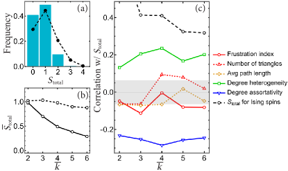
Figure 1: (a) Bars show the distribution of total spin in the ground state of $\mathcal{N}=916$ random graphs with $N=30$ qubits and $N_{e}=45$ bonds with equal antiferromagnetic Heisenberg coupling. The dashed curve shows $S_{\text{total}}$ for Ising spins. (b) Ensemble average of $S_{\text{total}}$ vs average degree $\bar{k}=2N_{e}/N$ with $\mathcal{N}\approx 924$. (c) Correlation with various graph metrics. Points inside the gray band are statistically insignificant.

The strongest correlation seen in Fig. 1(c) is with the total spin for (classical) Ising spins on the same network. The latter is given by an optimal bipartition (also known as the max-cut problem [51, 8]), where one divides the spins into two oppositely aligned groups $A$ and $B$ so as to maximize the number of $A$-$B$ bonds. As shown in Fig. 1, this bipolar state overestimates $S_{\text{total}}$ for the Heisenberg spins, especially at larger $\bar{k}$. Nonetheless, it is useful for interpreting some of the results.

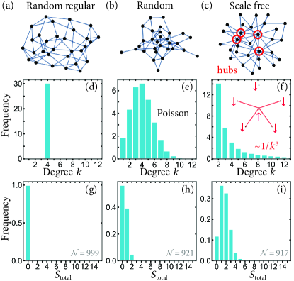
Figure 2: Sample graph (top), degree distribution (middle), and $S_{\text{total}}$ distribution (bottom) for random regular, random, and scale-free Barabási-Albert networks with $N=30$ and $\bar{k}\approx 4$. The power-law tail in (f) gives rise to hubs [circled in (c)] that want to polarize their neighborhoods, as shown in the inset.

Importance of heterogeneity.—Suppressing heterogeneity results in the family of random regular graphs, where each spin has the same degree $k$. Figure 2(g) shows that for $k=3$ one almost always (more than $98\%$ of the cases) has $S_{\text{total}}=0$, and the same holds for $k>3$ (see Supplement [49]). This strong result shows that heterogeneity is essential for a nonzero total spin. Conversely, one can ramp up the heterogeneity by producing scale-free graphs [53] where the degree distribution $p_{k}$ follows a power law. A well known example is the Barabási-Albert model [54], for which $p_{k}\sim 1/k^{3}$. As shown in Fig. 2(i), these graphs exhibit much higher magnetizations. The enhancement can be understood as originating from “hubs,” i.e., nodes with a disproportionately high degree. Such hubs form a locally star structure, favoring a net spin imbalance [see Fig. 2(f) inset]. As we discuss below, this effect persists when hubs are embedded in a broader class of networks.

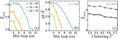
Figure 3: (a) Average total spin and (b) heterogeneity, given by the standard deviation $\Delta k$ of the degree distribution, for random graphs without short loops and $N=30$. (c) $\bar{S}_{\text{total}}$ for Barabási-Albert graphs with $N=30$, $\bar{k}=3.8$, and tunable number of triangles, measured by the mean clustering coefficient $C\in[0,1]$ [5]. Dashed curve shows $\bar{S}_{\text{total}}$ for Ising spins.

Insensitivity to frustration.—An alternative argument for the unmagnetized nature of random regular graphs [Fig. 2(g)] could be that they have fewer short loops compared to random graphs [55, 56], so they appear locally treelike. Thus, $S_{\text{total}}$ is small due to lack of frustration, not because of homogeneity. To test this proposition, we directly vary the number of short loops in two different ways and see its effect on $S_{\text{total}}$: First, we uniformly sample from random graphs without loops of up to a given size $l$ [57]. We find that the total-spin distribution is almost unaffected by removing all triangles ($l=3$). As $l$ is increased further, $\bar{S}_{\text{total}}$ eventually drops to zero at some threshold $l=l_{c}$ [Fig. 3(a)]; however, $l_{c}$ depends strongly on the number of bonds $N_{e}$ and $\bar{S}_{\text{total}}$ does not appear to be sensitive as to whether $l$ is even or odd. Instead, it follows the variation in the degree distribution, which becomes progressively narrower with the removal of short loops [Fig. 3(b)]. Thus, we infer that $S_{\text{total}}$ is dictated by the heterogeneity and not by the frustration. Second, we follow Ref. [58] to augment the Barabási-Albert model with a triangle formation step, which allows one to tune the number of triangles without changing the degree distribution or the assortativity. As shown in Fig. 3(c), this yields a weak variation of $\bar{S}_{\text{total}}$ which is reproduced by the optimal bipartition. We also find that $\bar{S}_{\text{total}}$ does not vary appreciably with shorter path lengths in small-world graphs (see Supplement [49]).

While this indifference to frustration may be counterintuitive, note the same holds on lattices, where both non-frustrated (e.g., square) and frustrated (e.g., Kagome) cases have $S_{\text{total}}=0$, albeit with very different magnetic order. Likewise, we expect frustration to be important in setting the order on general networks.

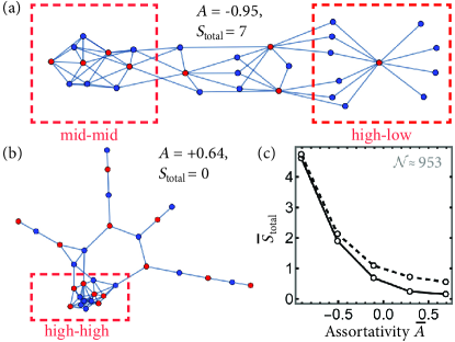
Figure 4: (a) Most disassortative and (b) most assortative networks with the same degree sequence. Node colors show a bipolar ground state of Ising spins. (b) Variation of $\bar{S}_{\text{total}}$ as the assortativity [6] is tuned for random graphs with $N=30$ and $\bar{k}=4$. Dashed curve shows the variation for Ising spins.

Importance of disassortativity.—Not all heterogeneous networks have large magnetization. Another key metric is the assortativity coefficient $A\in[-1,1]$ [6]. Perfect assortativity ($A=1$) requires all nodes to have the same degree (for which $S_{\text{total}}\simeq 0$), whereas perfect disassortativity ($A=-1$) occurs in a star graph and, more generally, in complete bipartite graphs with sublattice imbalance [59] (where $S_{\text{total}}$ can be large). Crucially, one can tune $A$ without altering the degrees via rewiring pairs of bonds [60, 61] or by solving a linear optimization problem [59]. Thus, Figs. 4(a) and 4(b) show two graphs with very different values of $A$ but the same degrees (hence, the same heterogeneity). The first graph is the most disassortative and has $S_{\text{total}}=7$, whereas the latter is the most assortative and has $S_{\text{total}}=0$. The physical origin of this large disparity becomes clear if one examines the structure of these networks [60]: Strongly disassortative graphs have a section where few high-degree nodes (hubs) connect to many low-degree nodes in an approximately bipartite structure [Fig. 4(a)], which gives rise to a large spin imbalance. By contrast, in strongly assortative graphs high-degree nodes form a tightly connected group and low-degree nodes form a treelike structure [Fig. 4(b)], neither of which favors a large magnetization. Note that the large $S_{\text{total}}$ in the former case requires both the presence of hubs and disassortativity.

Figure 4(c) shows that $\bar{S}_{\text{total}}$ falls sharply as we tune $A$ from its minimum to maximum value for random graphs. The same behavior is observed for Ising spins and for scale-free graphs (see Supplement [49]).

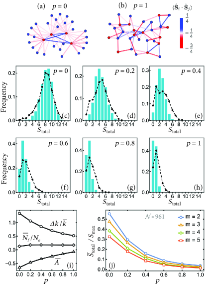
Figure 5: (a) Graph with embedded hubs and (b) graph with no hubs generated by the growth model described in text. Node colors show the ground state for Ising spins and bond colors show ground-state correlations for our Heisenberg model. (c)–(f) Variation of the total-spin distribution with the structure parameter $p$ for $N=30$ and $\bar{k}=3.8$. Dashed curves are for Ising spins. (i) Corresponding variation of heterogeneity $\Delta k$, frustration index $N_{f}$, and assortativity $A$. (j) Average total spin as a function of $p$ and $\bar{k}=2m-m(m+1)/N$ for $N=30$.

Tunable spin distribution.—Fortunately, we can use a simple model to grow networks with tunable heterogeneity and assortativity. It has a parameter $m\in\mathbb{Z}$ that sets the average degree and another parameter $p\in[0,1]$ that controls the structure. The protocol starts with a small clique of $m$ nodes, and in each step links a new node $i$ to $m$ existing nodes as follows: (1) Select an existing node $j$ at random, (2) with probability $p$ link $(i,j)$, (3) else link $i$ to a neighbor of $j$ with preferential attachment, i.e., with probability proportional to the neighbor’s degree. This is a variant of the “copy models” for the Web [62, 63, 64].

As shown in Fig. 5(a), for $p=0$ we get strongly disassortative graphs where many low-degree “outer” nodes connect to a few “central” hubs. As $p$ is increased to $1$, the graphs become more homogeneous [Fig. 5(b)]. Thus, both the heterogeneity and the disassortativity fall monotonically with $p$, while the frustration level varies weakly, as in Fig. 5(i). Accordingly, we find that the total-spin distribution is peaked at a macroscopic value of $O(N)$ for $p=0$ and moves toward zero as $p$ goes to $1$ [Figs. 5(c)-5(h)]. In addition, $\bar{S}_{\text{total}}$ decreases with the average degree $\bar{k}\approx 2m$ [Fig. 5(j)] as in random graphs.

In Fig. 5(c) the distribution is broad, covering almost the full range of $S_{\text{total}}$. Here, the maximum total spin occurs when all of the outer nodes link to the initial clique, producing a star configuration with $m$ giant central hubs [as in Fig. 6(a) without the outer ring]. For $N\gg m$ it is then energetically favorable to align the hub spins opposite to the outer spins, which gives $S_{\text{total}}=N/2-m$. However, during the growth stage a new node may connect to an outer node instead, which can then accumulate more bonds to become a mini hub, at the expense the initial clique which now has fewer bonds. In other words, the giant hubs can break into several smaller hubs, which then align opposite to the outer nodes [see Fig. 5(a)], reducing $S_{\text{total}}$. Note that the bonds between the hubs add frustration but do not change the total spin.

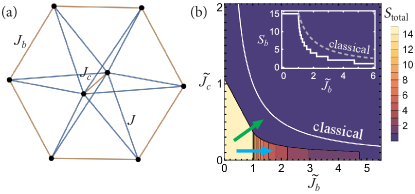
Figure 6: (a) Wheel graph with $2$ central spins and $N_{b}=6$ outer spins. (b) Phase diagram for $N_{b}=30$ and rescaled couplings $\tilde{J}_{b}\coloneqq 4J_{b}/(JN_{c})$ and $\tilde{J}_{c}\coloneqq J_{c}N_{c}/(JN_{b})$. Green arrow shows a discontinuous transition from a state where central and outer spins are oppositely aligned to a state where both add up to zero. Blue arrow shows a continuous transition where the net outer spin $S_{b}$ falls in steps of $1$ at a rate $\sim N_{b}(\tilde{J}_{b}-1)^{-1/2}$ (inset). This divergence is absent for classical Heisenberg spins (dashed curve), for which $S_{\text{total}}=0$ for $\tilde{J}_{b}\tilde{J}_{c}>1$ (solid curve).

Tuning $S_{\text{total}}$ in a non-random frustrated network.—Motivated by these results, we propose a simple wheel geometry where one can deterministically vary $S_{\text{total}}$ across its range by tuning some of the bond strengths, which may be easier to implement experimentally. The wheel consists of $N_{c}$ central spins with all-to-all coupling $J_{c}$, $N_{b}$ outer spins forming a ring with coupling $J_{b}$, and all bonds between the two sets of strength $J$, forming the spokes. Figure 6(a) shows a sketch for $N_{c}=2$ and $N_{b}=6$.

To understand its behavior, note that the spokes favor both the outer spin $S_{b}$ and the central spin $S_{c}$ to be large but anti-aligned, i.e., $S_{\text{total}}=|S_{b}-S_{c}|$, whereas $J_{b}$ and $J_{c}$ want to suppress $S_{b}$ and $S_{c}$, respectively. For simplicity, let us consider $N_{c}=2$ and $N_{b}$ even. Then the central spins form either a singlet or a triplet, depending on how strongly the central bonds compete with the spokes. For $J_{c}N_{c}^{2}\gg JN_{b}N_{c}$ we expect $S_{c}=0$, which reduces the network to just the ring, yielding $S_{b}=0$ and $S_{\text{total}}=0$. In contrast, for $J_{c}N_{c}^{2}\ll JN_{b}N_{c}$ we expect $S_{c}=1$, which leads to a competition between the spokes and the outer bonds: For $J_{b}N_{b}\ll JN_{b}N_{c}$ the outer spins align, so that $S_{b}=N_{b}/2$ and $S_{\text{total}}=N_{b}/2-1$, whereas for $J_{b}N_{b}\gg JN_{b}N_{c}$ they cancel, giving $S_{b}=0$ and $S_{\text{total}}=1$. Thus, by varying $J_{b}$ and $J_{c}$ one should be able to stabilize any total spin between $0$ and $N_{b}/2-1$.

These intuitions are confirmed by solving the system exactly using the Bethe Ansatz solution for the Heisenberg ring [65, 66] (see Supplement [49] for details). For $N_{c}=2$ this gives the phase diagram in Fig. 6(b). As expected, we find an extended antiferromagnetic region where $S_{b}=S_{c}=0$ and an extended ferromagnetic region where both spins are maximum but oppositely aligned. The two regions share a border where the magnetization collapses abruptly (green arrow). On the other hand, for small $J_{c}$ the outer spin falls in steps of $1$ with $J_{b}$, exhibiting a power-law diverging susceptibility at $J_{b}=JN_{c}/4$. Interestingly, this blow up is absent for classical Heisenberg spins (see Supplement [49]), for which $S_{\text{total}}$ is generally higher. For odd $N_{c}$ the center cannot form a singlet, so there is always a competition between $J$ and $J_{b}$, leading to a stepwise decrease of $S_{\text{total}}$ (see Supplement [49] for the phase diagram for $N_{c}=3$).

Outlook.—Perhaps the most promising platform for realizing our setup is ion traps, for which there are concrete protocols for engineering arbitrary pairwise Heisenberg coupling with existing technology for several tens of qubits [25, 26, 27]. A large class of networks can also be fabricated in photonic platforms [29, 30], where Heisenberg interactions may be simulated digitally [28, 35] or using tailored light-matter coupling [67]. Our results support the general view that hubs promote cohesion across a network [4] (e.g., ferromagnetic ordering [8, 68, 69, 70]), while pointing out the importance of assortativity [6, 71].

At the same time, they raise a number of open questions: (1) Why is $S_{\text{total}}$ insensitive to frustration? This is far from obvious and likely depends on the mechanism for magnetic interactions. In fact, preliminary calculations show that frustration strongly affects $S_{\text{total}}$ when magnetism arises from the delocalization of a doped carrier [72, 73]. (2) A related and perhaps the most crucial question concerns the nature of the ground state. Studies of classical Ising spins have found a glassy phase on small-world and scale-free networks [8, 74, 75, 76]. Are quantum fluctuations in the Heisenberg model strong enough to stabilize a spin liquid in the absence of a lattice symmetry [77]? (3) What are the dynamical and ergodicity properties and how are these affected by the network topology? (4) Is the magnetic order sensitive to motifs [78] other than hubs, or to community structures that regulate cooperative phenomena such as synchronization [71]? The latter arises in cluster magnetism [79]. (5) How does the physics change with bond disorder [8] or anisotropy? (6) As natural interactions decay with distance, it is useful to model spatial networks [9], which may be designed with Rydberg atoms in tweezers [80, 81]. Finally, we hope our findings herald broader explorations of quantum many-body networks beyond frustrated magnetism.

We thank Sitabhra Sinha and Sthitadhi Roy for useful discussions and comments. SD acknowledges use of the HPC facility at MPIPKS, Dresden.

Supplemental Material for
“Frustrated Quantum Magnetism on Complex Networks: What Sets the Total Spin”

Random trees

A tree has a bipartite structure [Fig. S1(a)], for which $S_{\text{total}}=|N_{A}-N_{B}|/2$, where $N_{A}$ and $N_{B}$ are the numbers of spins in the two sublattices. Figure S1(b) shows that both the average and the spread of $S_{\text{total}}$ over random trees with $N$ sites and $N-1$ bonds scale as $\sqrt{N}$.

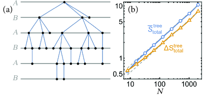
Figure S1: (a) Tree with $N=30$ sites. Horizontal lines show the two sublattices. (b) The average and the standard deviation of $S_{\text{total}}$ over $\mathcal{N}=1000$ random trees as a function of $N$. Dashed lines show the fits $0.23\sqrt{N}$ and $0.17\sqrt{N}$, respectively.

Random regular graphs

In the main text we showed that a random regular graph, where each node has $k=3$ neighbors, almost always has $S_{\text{total}}=0$. Figure S2 shows the same holds for $k=4$ and $k=5$, further demonstrating that heterogeneity is essential for nonzero total spin.

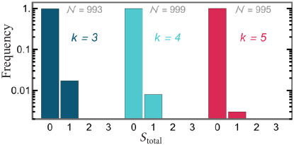
Figure S2: Total-spin distribution of random regular networks with $N=30$ sites for different values of the degree $k$.

Small-world networks

One can interpolate between a regular lattice and random graphs by randomly rewiring a small fraction of the bonds of the lattice; These “shortcuts” dramatically shorten the average path length between two nodes while maintaining a high clustering, resulting in a small-world character [1]. Figure S3 shows that this procedure leads to a slow increase of the average total spin, which is accompanied by a similar rise in the heterogeneity. Thus, we find no strong dependence of $S_{\text{total}}$ on the path length.

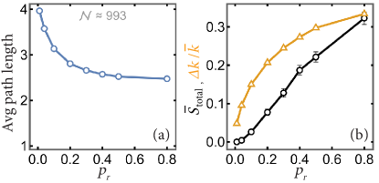
Figure S3: (a) Path length, (b) total spin and heterogeneity as a function of the rewiring probability $p_{r}$ for Watts-Strogatz graphs with $N=30$ and $\bar{k}=4$.

(Dis)assortative scale-free networks

In the main text we explained how tuning the assortativity of random graphs strongly affects $S_{\text{total}}$, which falls sharply with the assortativity coefficient $A$ [2]. Figure S4 shows the same is true for Barabási-Albert graphs with scale-free degree distribution ($p_{k}\sim 1/k^{3}$).

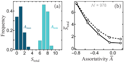
Figure S4: (a) Total-spin distribution of the most assortative ($\bar{A}=+0.17$) and the most disassortative ($\bar{A}=-0.78$) scale-free graphs with $N=30$ and $\bar{k}=3.8$. (b) Variation of $\bar{S}_{\text{total}}$ with the average assortativity. Dashed curve is for Ising spins.

Exact solution for the wheel

In the main text we proposed a wheel-shaped network where the total spin can be tuned by varying some of the bond strengths. The network consists of $N_{c}$ central spins and $N_{b}$ outer spins with the Hamiltonian

$$\hat{H}=\frac{J_{c}}{2}\hat{\mathbf{S}}_{c}^{2}+J\hat{\mathbf{S}}_{b}\cdot\hat{\mathbf{S}}_{c}+J_{b}\sum_{n=1}^{N_{b}}\hat{\mathbf{S}}_{n}\cdot\hat{\mathbf{S}}_{n+1}$$ (S1)

up to a constant, where $\hat{\mathbf{S}}_{c}$ is the net central spin, $\hat{\mathbf{S}}_{b}\coloneqq\sum_{i=1}^{N_{b}}\hat{\mathbf{S}}_{i}$ is the net outer spin, and $\hat{\mathbf{S}}_{N_{b}+1}\equiv\hat{\mathbf{S}}_{1}$. Below we describe exact solutions for the ground states of this network for both classical and quantum spins.

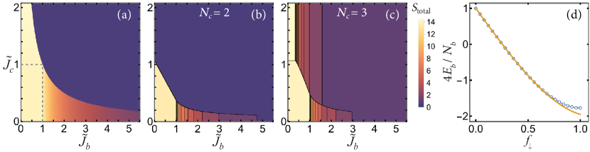
Figure S5: Phase diagram of the wheel-shaped network introduced in the main text [Eq. (S1)] for (a) classical spins with $N_{c}=2$, $N_{b}=30$, (b) qubits with $N_{c}=2$, $N_{b}=30$, and (c) qubits with $N_{c}=3$, $N_{b}=30$. (d) Minimum energy of the Heisenberg ring as a function of twice the fraction of $\downarrow$ spins for $N_{b}=50$. Orange curve shows the fit $1-4f_{\downarrow}+1.05f_{\downarrow}^{3}$.

Classical spins

In order to lower energy $\mathbf{S}_{b}$ and $\mathbf{S}_{c}$ point in opposite directions. Without loss of generality we take $\mathbf{S}_{b}$ along $+z$ and $\mathbf{S}_{c}$ along $-z$. The maximum magnitude of $\mathbf{S}_{c}$ is $N_{c}S$, where $S$ is the magnitude of each spin. To compare with qubits we set $S=1/2$ and write $\mathbf{S}_{c}=-(N_{c}/2)u\hat{\mathbf{z}}$, where $u\in[0,1]$. This central spin acts as an effective magnetic field for the Heisenberg ring [see Eq. (S1)], whose thermodynamic properties can be solved exactly [3]. The field wants to polarize the spins along $+z$, whereas the bonds prefer a Néel-type antiferromagnet. In the ground state, the spins orient along the polar and azimuthal angles

$$\theta_{n} =\theta\;,$$ (S2a)

$$\phi_{n} =n(\pi-\alpha)+\phi_{0}\;,$$ (S2b)

where $\theta$ goes from $0$ to $\pi/2$ as the field decreases, $\phi_{0}$ is an arbitrary constant, and $\alpha=\big{[}1-(-1)^{N_{b}}\big{]}\pi/(2N_{b})$. Substituting these into the Hamiltonian gives the energy

$$\tilde{E}=\tilde{J}_{c}u^{2}-2uv+\tilde{J}_{b}\cos^{2}(\alpha/2)v^{2}\;,$$ (S3)

where $v\coloneqq\cos\theta$, $\tilde{E}\coloneqq 8E/(JN_{b}N_{c})$, $\tilde{J}_{c}\coloneqq J_{c}N_{c}/(JN_{b})$, and $\tilde{J}_{b}\coloneqq 4J_{b}/(JN_{c})$. Minimizing $\tilde{E}$ with respect to the fractions $u$ and $v$ yields a ground state with $S_{b}=\frac{1}{2}N_{b}v$, $S_{c}=\frac{1}{2}N_{c}u$, and $S_{\text{total}}=\frac{1}{2}|N_{b}v-N_{c}u|$.

The resulting phase diagram comprises four regions:

$$u=v=0\quad \text{if }\tilde{J}_{c}\tilde{J}_{b}^{\prime}>1\;,$$ (S4a)

$$u=v=1\quad \text{if }\tilde{J}_{c}<1\text{ and }\tilde{J}_{b}^{\prime}<1\;,$$ (S4b)

$$u=1,v=1/\tilde{J}_{b}^{\prime}\quad \text{if }\tilde{J}_{c}\tilde{J}_{b}^{\prime}<1\text{ and }\tilde{J}_{b}^{\prime}>1\;,$$ (S4c)

$$v=1,u=1/\tilde{J}_{c}\quad \text{if }\tilde{J}_{c}\tilde{J}_{b}^{\prime}<1\text{ and }\tilde{J}_{c}>1\;,$$ (S4d)

with $\tilde{J}_{b}^{\prime}\coloneqq\tilde{J}_{b}\cos^{2}(\alpha/2)$, as shown in Fig. S5(a) for $N_{b}\gg N_{c}$. Note that $\alpha\approx 0$ for large $N_{b}$ and the phase diagram does not depend on whether $N_{c}$ is odd or even.

Quantum spins

Since $\hat{\mathbf{S}}_{b}^{2}$ and $\hat{\mathbf{S}}_{c}^{2}$ commute with $\hat{H}$ and $S_{\text{total}}=S_{bc}\coloneqq|S_{b}-S_{c}|$ in the ground state(s), we can write the lowest energy for a given $S_{b}$ and $S_{c}$ as

$$E=\frac{J_{c}}{2}\hat{S}_{c}^{2}+\frac{J}{2}\big{(}\hat{S}_{bc}^{2}-\hat{S}_{b}^{2}-\hat{S}_{c}^{2}\big{)}+J_{b}E_{b}(N_{b},S_{b})\;,$$ (S5)

where $\hat{S}^{2}\coloneqq S(S+1)$ and $E_{b}$ is the lowest energy of the Heisenberg ring. The latter can be found using the Bethe Ansatz [4], which involves solving the equations

$$N_{b}\tan^{-1}(2\lambda_{i})=\pi I_{i}+\sum_{j}\tan^{-1}(\lambda_{i}-\lambda_{j})$$ (S6)

for the rapidities $\lambda_{i}$, $i=1,2,\dots,N_{\downarrow}=N_{b}/2-S_{b}$, where $I_{i}=i-(N_{\downarrow}+1)/2$ for even $N_{b}$ and $i-(N_{\downarrow}+1\pm 1)/2$ for odd $N_{b}$ [5], whereupon $E_{b}=N_{b}/4-\sum_{i}2/(4\lambda_{i}^{2}+1)$. The two sets of $\{I_{i}\}$ for odd $N_{b}$ are degenerate in energy [6]. The ground-state spins are obtained by minimizing $E$ in Eq. (S5) over all quantum numbers $S_{b}=N_{b}/2,N_{b}/2-1,\dots$ and $S_{c}=N_{c}/2,N_{c}/2-1,\dots$.

Figures S5(b) and S5(c) show that the resulting phase diagram differs qualitatively for $N_{c}=2$ and $N_{c}=3$. As explained in the main text, this is because for odd $N_{c}$ one cannot have $S_{c}=0$, which leads to a stepwise fall of $S_{b}$ as $J_{b}$ is increased relative to $J$. To understand this feature more precisely we consider the energy as a function of $S_{b}$ for a given $S_{c}<S_{b}$,

$$\tilde{E}=\text{constant}+\frac{4S_{c}}{N_{c}}f_{\downarrow}+\frac{\tilde{J}_{b}}{2}\tilde{E}_{b}(f_{\downarrow})\;,$$ (S7)

where $f_{\downarrow}\coloneqq 1-2S_{b}/N_{b}$ is twice the fraction of $\downarrow$ spins in the ring, and $\tilde{E}_{b}\coloneqq 4E_{b}/N_{b}$. For large $S_{b}$ (small $f_{\downarrow}$) one can write $\tilde{E}_{b}\approx 1-4f_{\downarrow}+\eta f_{\downarrow}^{3}$, where $\eta\sim O(1)$ [Fig. S5(d)], which predicts the minimum energy for

$$f_{\downarrow}\approx\big{[}4\big{(}\tilde{J}_{b}-\tilde{J}_{b}^{*}\big{)}/\big{(}3\eta\tilde{J}_{b}\big{)}\big{]}^{1/2}$$ (S8)

when $\tilde{J}_{b}>\tilde{J}_{b}^{*}\coloneqq 2S_{c}/N_{c}$. Consequently, the susceptibility $\partial S_{b}/\partial\tilde{J}_{b}$ diverges as

$$\frac{\partial S_{b}}{\partial\tilde{J}_{b}}\approx-\frac{N_{b}}{2\sqrt{3\eta}\tilde{J}_{b}^{*}}\bigg{(}\frac{\tilde{J}_{b}}{\tilde{J}_{b}^{*}}-1\bigg{)}^{\!-1/2},$$ (S9)

which is seen in Fig. S5(b) for $S_{c}=1$ and in Fig. S5(c) for $S_{c}=3/2,1/2$. No such divergence is present for classical spins [Fig. S5(a)].

Quantum vs. classical $S_{\text{total}}$

Figure S6 shows a comparison between the total spins of classical and quantum Heisenberg models defined on two types of networks: (i) random graphs and (ii) graphs generated by the copy model introduced in the main text, where heterogeneity and assortativity can be tuned by varying a structure parameter $p$. Generally, we find that the two spins are highly correlated and that the classical total spin is larger by $O(1)$.

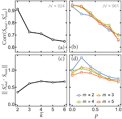
Figure S6: (Top panel) Correlation and (bottom panel) root-mean-square deviation between the net magnetizations of classical and quantum spins for random graphs (left column) and graphs generated by the growth model introduced in the main text (right column) with $N=30$ sites.

References

- Strogatz [2001] S. H. Strogatz, Exploring complex networks, Nature (London) 410, 268 (2001).
- Newman [2018] M. E. J. Newman, Networks: An Introduction (Oxford University Press, Oxford, UK, 2018).
- da Mata [2020] A. S. da Mata, Complex networks: a mini-review, Braz. J. Phys. 50, 658 (2020).
- Barrat et al. [2008] A. Barrat, M. Barthelemy, and A. Vespignani, Dynamical Processes on Complex Networks (Cambridge University Press, Cambridge, UK, 2008).
- Watts and Strogatz [1998] D. J. Watts and S. H. Strogatz, Collective dynamics of ‘small-world’ networks, Nature (London) 393, 440 (1998).
- Newman [2002] M. E. J. Newman, Assortative mixing in networks, Phys. Rev. Lett. 89, 208701 (2002).
- Newman [2011] M. E. J. Newman, Communities, modules and large-scale structure in networks, Nat. Phys. 8, 25 (2011).
- Dorogovtsev et al. [2008] S. N. Dorogovtsev, A. V. Goltsev, and J. F. F. Mendes, Critical phenomena in complex networks, Rev. Mod. Phys. 80, 1275 (2008).
- Boccaletti et al. [2006] S. Boccaletti, V. Latora, Y. Moreno, M. Chavez, and D. Hwang, Complex networks: Structure and dynamics, Phys. Rep. 424, 175 (2006).
- Albert and Barabási [2002] R. Albert and A.-L. Barabási, Statistical mechanics of complex networks, Rev. Mod. Phys. 74, 47 (2002).
- D’Souza et al. [2019] R. M. D’Souza, J. Gómez-Gardeñes, J. Nagler, and A. Arenas, Explosive phenomena in complex networks, Adv. Phys. 68, 123 (2019).
- Boccaletti et al. [2016] S. Boccaletti, J. A. Almendral, S. Guan, I. Leyva, Z. Liu, I. Sendiña Nadal, Z. Wang, and Y. Zou, Explosive transitions in complex networks’ structure and dynamics: Percolation and synchronization, Phys. Rep. 660, 1 (2016).
- Mülken and Blumen [2011] O. Mülken and A. Blumen, Continuous-time quantum walks: Models for coherent transport on complex networks, Phys. Rep. 502, 37 (2011).
- Berkovits [2008] R. Berkovits, Localisation of optical modes in complex networks, Eur. Phys. J. Special Topics 161, 259 (2008).
- Tikhonov and Mirlin [2021] K. S. Tikhonov and A. D. Mirlin, From Anderson localization on random regular graphs to many-body localization, Ann. Phys. (Amsterdam) 435, 168525 (2021).
- Nokkala et al. [2023] J. Nokkala, J. Piilo, and G. Bianconi, Complex quantum networks: a topical review, arXiv:2311.16265 (2023).
- Biamonte et al. [2019] J. Biamonte, M. Faccin, and M. De Domenico, Complex networks from classical to quantum, Commun. Phys. 2, 53 (2019).
- Halu et al. [2012] A. Halu, L. Ferretti, A. Vezzani, and G. Bianconi, Phase diagram of the Bose-Hubbard model on complex networks, Europhys. Lett. 99, 18001 (2012).
- Halu et al. [2013] A. Halu, S. Garnerone, A. Vezzani, and G. Bianconi, Phase transition of light on complex quantum networks, Phys. Rev. E 87, 022104 (2013).
- Ostilli [2020] M. Ostilli, Absence of small-world effects at the quantum level and stability of the quantum critical point, Phys. Rev. E 102, 052126 (2020).
- Bentsen et al. [2019] G. Bentsen, T. Hashizume, A. S. Buyskikh, E. J. Davis, A. J. Daley, S. S. Gubser, and M. Schleier-Smith, Treelike interactions and fast scrambling with cold atoms, Phys. Rev. Lett. 123, 130601 (2019).
- Hartmann et al. [2019] J.-G. Hartmann, J. Murugan, and J. P. Shock, Chaos and scrambling in quantum small worlds, arXiv:1901.04561 (2019).
- Sundar et al. [2021] B. Sundar, M. Walschaers, V. Parigi, and L. D. Carr, Response of quantum spin networks to attacks, J. Phys. Complex. 2, 035008 (2021).
- Monroe et al. [2021] C. Monroe, W. C. Campbell, L.-M. Duan, Z.-X. Gong, A. V. Gorshkov, P. W. Hess, R. Islam, K. Kim, N. M. Linke, G. Pagano, P. Richerme, C. Senko, and N. Y. Yao, Programmable quantum simulations of spin systems with trapped ions, Rev. Mod. Phys. 93, 025001 (2021).
- Korenblit et al. [2012] S. Korenblit, D. Kafri, W. C. Campbell, R. Islam, E. E. Edwards, Z.-X. Gong, G.-D. Lin, L.-M. Duan, J. Kim, K. Kim, and C. Monroe, Quantum simulation of spin models on an arbitrary lattice with trapped ions, New J. Phys. 14, 095024 (2012).
- Teoh et al. [2020] Y. H. Teoh, M. Drygala, R. G. Melko, and R. Islam, Machine learning design of a trapped-ion quantum spin simulator, Quantum Sci. Tech. 5, 024001 (2020).
- Davoudi et al. [2020] Z. Davoudi, M. Hafezi, C. Monroe, G. Pagano, A. Seif, and A. Shaw, Towards analog quantum simulations of lattice gauge theories with trapped ions, Phys. Rev. Res. 2, 023015 (2020).
- Lamata et al. [2018] L. Lamata, A. Parra-Rodriguez, M. Sanz, and E. Solano, Digital-analog quantum simulations with superconducting circuits, Adv. Phys. X 3, 1457981 (2018).
- Tsomokos et al. [2010] D. I. Tsomokos, S. Ashhab, and F. Nori, Using superconducting qubit circuits to engineer exotic lattice systems, Phys. Rev. A 82, 052311 (2010).
- Kollár et al. [2019] A. J. Kollár, M. Fitzpatrick, P. Sarnak, and A. A. Houck, Line-graph lattices: Euclidean and non-Euclidean flat bands, and implementations in circuit quantum electrodynamics, Commun. Math. Phys. 376, 1909 (2019).
- Onodera et al. [2020] T. Onodera, E. Ng, and P. L. McMahon, A quantum annealer with fully programmable all-to-all coupling via Floquet engineering, npj Quantum Inf. 6, 48 (2020).
- King et al. [2023] A. D. King et al., Quantum critical dynamics in a 5,000-qubit programmable spin glass, Nature 617, 61 (2023).
- Lechner et al. [2015] W. Lechner, P. Hauke, and P. Zoller, A quantum annealing architecture with all-to-all connectivity from local interactions, Sci. Adv. 1, e1500838 (2015).
- Qiu et al. [2020] X. Qiu, P. Zoller, and X. Li, Programmable quantum annealing architectures with Ising quantum wires, PRX Quantum 1, 020311 (2020).
- Hung et al. [2016] C.-L. Hung, A. González-Tudela, J. I. Cirac, and H. J. Kimble, Quantum spin dynamics with pairwise-tunable, long-range interactions, Proc. Natl. Acad. Sci. U.S.A. 113, E4946 (2016).
- McMahon et al. [2016] P. L. McMahon, A. Marandi, Y. Haribara, R. Hamerly, C. Langrock, S. Tamate, T. Inagaki, H. Takesue, S. Utsunomiya, K. Aihara, R. L. Byer, M. M. Fejer, H. Mabuchi, and Y. Yamamoto, A fully programmable 100-spin coherent ising machine with all-to-all connections, Science 354, 614 (2016).
- Fung et al. [2023] F. Fung, E. Rosenfeld, J. D. Schaefer, A. Kabcenell, J. Gieseler, T. X. Zhou, T. Madhavan, N. Aslam, A. Yacoby, and M. D. Lukin, Programmable quantum processors based on spin qubits with mechanically-mediated interactions and transport, arXiv:2307.12193 (2023).
- Schlipf et al. [2017] L. Schlipf, T. Oeckinghaus, K. Xu, D. B. R. Dasari, A. Zappe, F. F. de Oliveira, B. Kern, M. Azarkh, M. Drescher, M. Ternes, K. Kern, J. Wrachtrup, and A. Finkler, A molecular quantum spin network controlled by a single qubit, Sci. Adv. 3, e1701116 (2017).
- Lacroix et al. [2011] C. Lacroix, P. Mendels, and F. Mila, eds., Introduction to Frustrated Magnetism: Materials, Experiments, Theory, Vol. 164 (Springer, New York, 2011).
- Diep [2013] H. T. Diep, ed., Frustrated Spin Systems (World Scientific, Singapore, 2013).
- Moessner and Ramirez [2006] R. Moessner and A. P. Ramirez, Geometrical frustration, Phys. Today 59, 24 (2006).
- Zheng et al. [2014] X. Zheng, D. Zeng, and F.-Y. Wang, Social balance in signed networks, Inf. Syst. Front. 17, 1077 (2014).
- Lieb and Mattis [1962] E. Lieb and D. Mattis, Ordering energy levels of interacting spin systems, J. Math. Phys. 3, 749 (1962).
- Savary and Balents [2016] L. Savary and L. Balents, Quantum spin liquids: a review, Rep. Prog. Phys. 80, 016502 (2016).
- Zhou et al. [2017] Y. Zhou, K. Kanoda, and T.-K. Ng, Quantum spin liquid states, Rev. Mod. Phys. 89, 025003 (2017).
- Lancaster [2023] T. Lancaster, Quantum spin liquids, arXiv:2310.19577 (2023).
- Schollwöck [2011] U. Schollwöck, The density-matrix renormalization group in the age of matrix product states, Ann. Phys. 326, 96 (2011).
- Fishman et al. [2022] M. Fishman, S. White, and E. Stoudenmire, The ITensor software library for tensor network calculations, SciPost Phys. Codebases , 4 (2022).
- [49] See Supplemental Material, which includes Refs. [82, 83], for statistics of the total spin on random trees, random regular graphs, scale-free graphs with tunable assortativity, comparison with classical spins, and exact solutions for the wheel for classical and quantum spins.
- Aref and Wilson [2017] S. Aref and M. C. Wilson, Measuring partial balance in signed networks, J. Complex Netw. 6, 566 (2017).
- Holme et al. [2003] P. Holme, F. Liljeros, C. R. Edling, and B. J. Kim, Network bipartivity, Phys. Rev. E 68, 056107 (2003).
- Aref and Wilson [2018] S. Aref and M. C. Wilson, Balance and frustration in signed networks, J. Complex Netw. 7, 163 (2018).
- Caldarelli [2007] G. Caldarelli, Scale-Free Networks: Complex Webs in Nature and Technology (Oxford University Press, Oxford, UK, 2007).
- Barabási and Albert [1999] A.-L. Barabási and R. Albert, Emergence of scaling in random networks, science 286, 509 (1999).
- Wormald [1981] N. C. Wormald, The asymptotic distribution of short cycles in random regular graphs, J. Comb. Theory, Ser. B 31, 168 (1981).
- Bonneau et al. [2017] H. Bonneau, A. Hassid, O. Biham, R. Kühn, and E. Katzav, Distribution of shortest cycle lengths in random networks, Phys. Rev. E 96, 062307 (2017).
- Bayati et al. [2018] M. Bayati, A. Montanari, and A. Saberi, Generating random networks without short cycles, Oper. Res. 66, 1227 (2018).
- Holme and Kim [2002] P. Holme and B. J. Kim, Growing scale-free networks with tunable clustering, Phys. Rev. E 65, 026107 (2002).
- Van Mieghem et al. [2010] P. Van Mieghem, H. Wang, X. Ge, S. Tang, and F. A. Kuipers, Influence of assortativity and degree-preserving rewiring on the spectra of networks, Eur. Phys. J. B 76, 643 (2010).
- Xulvi-Brunet and Sokolov [2005] R. Xulvi-Brunet and I. M. Sokolov, Changing correlations in networks: assortativity and dissortativity, Acta Phys. Pol. B 36, 1431 (2005).
- Noldus and Van Mieghem [2015] R. Noldus and P. Van Mieghem, Assortativity in complex networks, J. Complex Netw. 3, 507 (2015).
- Kleinberg et al. [1999] J. M. Kleinberg, R. Kumar, P. Raghavan, S. Rajagopalan, and A. S. Tomkins, The web as a graph: Measurements, models, and methods, in Computing and Combinatorics, Lecture Notes in Computer Science, Vol. 1627 (Springer, Berlin, 1999) pp. 1–17.
- Kumar et al. [2000] R. Kumar, P. Raghavan, S. Rajagopalan, D. Sivakumar, A. Tomkins, and E. Upfal, Stochastic models for the web graph, in Proceedings of the 41st IEEE Annual Symposium on Foundations of Computer Science (IEEE Computing Society, California, 2000) pp. 57–65.
- Alam et al. [2019] M. Alam, K. S. Perumalla, and P. Sanders, Novel parallel algorithms for fast multi-GPU-based generation of massive scale-free networks, Data Sci. Eng. 4, 61 (2019).
- Karbach et al. [1998] M. Karbach, K. Hu, and G. Müller, Introduction to the Bethe Ansatz II, Comput. Phys. 12, 565 (1998).
- Karbach and Mutter [1995] M. Karbach and K.-H. Mutter, The antiferromagnetic spin- 1/2 -XXZ model on rings with an odd number of sites, J. Phys. A 28, 4469 (1995).
- Kay and Angelakis [2008] A. Kay and D. G. Angelakis, Reproducing spin lattice models in strongly coupled atom-cavity systems, Europhys. Lett. 84, 20001 (2008).
- Bianconi [2012a] G. Bianconi, Enhancement of in the superconductor–insulator phase transition on scale-free networks, J. Stat. Mech. 2012, P07021 (2012a).
- Bianconi [2012b] G. Bianconi, Superconductor-insulator transition on annealed complex networks, Phys. Rev. E 85, 061113 (2012b).
- Bianconi [2013] G. Bianconi, Superconductor-insulator transition in a network of 2d percolation clusters, Europhys. Lett. 101, 26003 (2013).
- Rodrigues et al. [2016] F. A. Rodrigues, T. K. D. Peron, P. Ji, and J. Kurths, The Kuramoto model in complex networks, Phys. Rep. 610, 1 (2016).
- Tasaki [1998] H. Tasaki, From Nagaoka’s ferromagnetism to flat-band ferromagnetism and beyond: An introduction to ferromagnetism in the Hubbard model, Prog. Theor. Phys. 99, 489 (1998).
- Kim [2023] K.-S. Kim, Exact hole-induced resonating-valence-bond ground state in certain Hubbard models, Phys. Rev. B 107, L140401 (2023).
- Herrero [2008] C. P. Herrero, Antiferromagnetic ising model in small-world networks, Phys. Rev. E 77, 041102 (2008).
- Bartolozzi et al. [2006] M. Bartolozzi, T. Surungan, D. B. Leinweber, and A. G. Williams, Spin-glass behavior of the antiferromagnetic Ising model on a scale-free network, Phys. Rev. B 73, 224419 (2006).
- Herrero [2009] C. P. Herrero, Antiferromagnetic Ising model in scale-free networks, Eur. Phys. J. B 70, 435 (2009).
- Balents [2010] L. Balents, Spin liquids in frustrated magnets, Nature (London) 464, 199 (2010).
- Milo et al. [2002] R. Milo, S. Shen-Orr, S. Itzkovitz, N. Kashtan, D. Chklovskii, and U. Alon, Network motifs: Simple building blocks of complex networks, Science 298, 824 (2002).
- Silveira et al. [2021] A. Silveira, R. Erichsen, and S. G. Magalhães, Geometrical frustration and cluster spin glass with random graphs, Phys. Rev. E 103, 052110 (2021).
- Morgado and Whitlock [2021] M. Morgado and S. Whitlock, Quantum simulation and computing with Rydberg-interacting qubits, AVS Quantum Sci. 3, 023501 (2021).
- Scholl et al. [2022] P. Scholl, H. J. Williams, G. Bornet, F. Wallner, D. Barredo, L. Henriet, A. Signoles, C. Hainaut, T. Franz, S. Geier, A. Tebben, A. Salzinger, G. Zürn, T. Lahaye, M. Weidemüller, and A. Browaeys, Microwave engineering of programmable Hamiltonians in arrays of Rydberg atoms, PRX Quantum 3, 020303 (2022).
- Blume et al. [1975] M. Blume, P. Heller, and N. A. Lurie, Classical one-dimensional Heisenberg magnet in an applied field, Phys. Rev. B. 11, 4483 (1975).
- Bärwinkel et al. [2000] K. Bärwinkel, H.-J. Schmidt, and J. Schnack, Ground-state properties of antiferromagnetic Heisenberg spin rings, J. Magn. Magn. Mater. 220, 227 (2000).

References

- Watts and Strogatz [1998] D. J. Watts and S. H. Strogatz, Collective dynamics of ‘small-world’ networks, Nature (London) 393, 440 (1998).
- Newman [2002] M. E. J. Newman, Assortative mixing in networks, Phys. Rev. Lett. 89, 208701 (2002).
- Blume et al. [1975] M. Blume, P. Heller, and N. A. Lurie, Classical one-dimensional Heisenberg magnet in an applied field, Phys. Rev. B. 11, 4483 (1975).
- Karbach et al. [1998] M. Karbach, K. Hu, and G. Müller, Introduction to the Bethe Ansatz II, Comput. Phys. 12, 565 (1998).
- Karbach and Mutter [1995] M. Karbach and K.-H. Mutter, The antiferromagnetic spin- 1/2 -XXZ model on rings with an odd number of sites, J. Phys. A 28, 4469 (1995).
- Bärwinkel et al. [2000] K. Bärwinkel, H.-J. Schmidt, and J. Schnack, Ground-state properties of antiferromagnetic Heisenberg spin rings, J. Magn. Magn. Mater. 220, 227 (2000).