Deep unfolding Network for Hyperspectral Image Super-Resolution with Automatic Exposure Correction

Abstract

In recent years, the fusion of high spatial resolution multispectral image (HR-MSI) and low spatial resolution hyperspectral image (LR-HSI) has been recognized as an effective method for HSI super-resolution (HSI-SR). However, both HSI and MSI may be acquired under extreme conditions such as night or poorly illuminating scenarios, which may cause different exposure levels, thereby seriously downgrading the yielded HSISR. In contrast to most existing methods based on respective low-light enhancements (LLIE) of MSI and HSI followed by their fusion, a deep Unfolding HSI Super-Resolution with Automatic Exposure Correction (UHSR-AEC) is proposed, that can effectively generate a high-quality fused HSI-SR (in texture and features) even under very imbalanced exposures, thanks to the correlation between LLIE and HSI-SR taken into account. Extensive experiments are provided to demonstrate the state-of-the-art overall performance of the proposed UHSR-AEC, including comparison with some benchmark peer methods.

Index Terms—  Hyperspectral image, exposure correction, super-resolution, deep unfolding

1 Introduction

Hyperspectral image (HSI) can capture the continuous spectral detection signal at individual pixel locations of an object [1, 2]. With rich information from hundreds of spectral bands, it has been widely used in remote sensing for target recognition [3], geological surveying [4], etc. Owing to limited solar irradiance and hardware, there exists a compromise between the spatial and spectral resolution of HSI [5]. In contrast, normally multispectral image (MSI) has higher spatial resolution and lower acquisition difficulty than HSI. Fusion of MSI and HSI has been regarded as an effective HSI super-resolution (HSI-SR) approach [6].

Hyperspectral sensors need to capture high quality HSI throughout the day. However, under extreme conditions such as night or poorly illuminating scenarios, the captured HSI and MSI are usually affected by low visibility, spectral distortion, etc., consequently degrading the spatial and spectral information quality and thus compromising the subsequent applications [7]. At the same time, due to the different sensing methods used by hyperspectral cameras and multispectral cameras, it is difficult to maintain the same exposure level for both HSI and MSI [8, 9], thereby seriously affecting the quality of useful information in HSI and MSI, such that existing HSI-SR methods cannot perform effectively. One possible approach is to perform low-light image enhancement (LLIE) on both HSI and MSI, separately, and then carry out HSI-SR. However, this approach treats LLIE and HSI-SR as two independent problems without considering their mutual effects in nature. This motivates our study for a new HSI-SR model that can mine mutual correlation, priors, and causal effects between LLIE and HSI-SR.

Existing HSI-SR methods can be categorized into two groups: model-based methods and deep learning-based methods. Model-based methods are based on the linear observation model linking the observed image and the original image, which relies on manually setting priors canonical rules. Yokoya et el. [10] proposed a coupled nonnegative matrix factorization to estimate the abundance matrix and endmember of the HSI; Dong et al. [11] converted the estimation of HSI into a joint estimation of dictionary and sparse coding through the spectral sparsity of HSI; Dian et el. [12] proposed a novel subspace-based low tensor multi-rank regularization method for HSI-SR. While model-based methods have explanations based on theoretical foundations, they often have poor performance due to their limited priors in well-defined mathematical forms. Deep learning methods have been widely used in HSI-SR in recent years. Xie et el. [8] proposed an unfolding-based network by combining the low-rank prior and generalized model of HSI; Zhang et el. [13] proposed a blind fusion network, which can overcome the mismatch between spectral and spatial responses. However, most existing HSI-SR methods have not yet seriously considered the degradation of complex environments, and the conditions for application are relatively limited. How to design new models to make HSI-SR applicable in complex environments is still an unsolved problem.

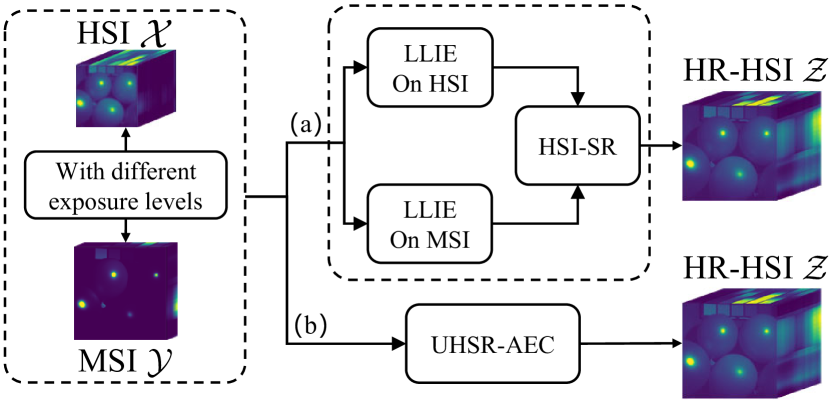
Fig. 1: Block diagram of generating HR-HSI $\cal Z$ from the acquired HSI $\cal X$ and MSI $\cal Y$ under different exposure levels, for (a) most existing methods and (b) the proposed UHSR-AEC.

Low-light image enhancement methods on natural images can be categorized into two groups: model-based methods and deep learning-based methods. Model-based LLIE methods focus on the statistical characteristics of the data. Ibrahim et al. [14] proposed a brightness-preserving dynamic histogram equalization method; Jobson et el. [15] used the Retinex theory in the field of image brightness enhancement. However, hand-picked constraints often limit reconstruction performance, especially in challenging light-degraded scenes. Meanwhile, many deep learning-based methods have been widely applied to the LLIE field in recent years. Chen et el. [16] proposed a deep network structure based on Retinex theory; Wu et el. [17] combined deep unfolding and Retinex theory to good effect; Wang et el. [18] proposed a diffusion-based network structure and a denoising process based on a physical exposure model, which can accurately capture noise and exposure. Deep learning-based LLIE methods are gradually becoming mainstream and have shown amazing performance. Since image enhancement methods on natural images do not take into account the spectral correlation of HSI, proposing an image enhancement method suitable for HSI remains an open challenge.

To solve the above problems, we propose a new HSI-SR restoration model, which integrates LLIE and SR, and can solve the HSI fusion in different exposure scenarios, as shown in Fig. 1. At the same time, we design a deep unfolding method, which integrates the advantages of the model-based method and the deep learning-based method, and can solve the above problems.

The main contributions are summarized as follows:

1. By integrating the LLIE and SR problems of HSI, a new HSI-SR degradation and recovery model is proposed, which is essential to solving the problem of different exposures in HSI fusion. Then a novel deep Unfolding HSI Super-Resolution method with Automatic Exposure Correction (UHSR-AEC) based on deep unfolding is proposed to solve the problem.

2. The proposed UHSR-AEC trains the considered model by solving three sub-problems (each with a data-fitting error and a regularizer) that are solved by the proximal gradient descent (PGD) algorithm, together with an Initialization Module (IM) for preserving details and texture features in HSI-SR.

3. Extensive experiments are performed to demonstrate the effectiveness of the proposed UHSR-AEC, including its state-of-the-art HSI-SR fusion performance and comparison with some existing benchmark LLIE-SR based methods.

2 NOTATIONS AND PROBLEM FORMULATION

2.1 Notations

In this paper, a scalar, a vector, a matrix, and a tensor are denoted by lowercase $x$, boldface lowercase $\mathbf{x}$, boldface capital $\mathbf{X}$, and calligraphic $\mathcal{X}$, respectively. $\mathbf{C}=\mathbf{A}\circ\mathbf{B}$ denotes the matrix-formed element-wise multiplication of $\mathbf{A}$ and $\mathbf{B}$, where matrices $\mathbf{A}$, $\mathbf{B}$, and $\mathbf{C}$ have the same dimension. $\|\mathbf{A}\|_{\text{F}}$ and $\|\mathbf{A}\|_{1}$ denote Frobenius norm and $\ell_{1}$ norm of matrix $\mathbf{A}$, respectively. For a tensor $\mathcal{X}\in\mathbb{R}^{I_{1}\times I_{2}\times\cdots\times I_{N}}$, the mode-$i$ unfolding martix is defined as $\mathbf{X}_{(i)}\in\mathbb{R}^{I_{i}\times\prod_{j\neq i}I_{j}}$.

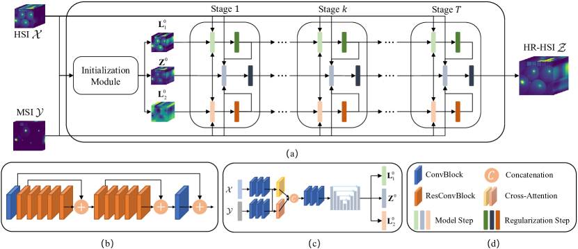
Fig. 2: (a) The proposed UHSR-AEC, which consists of Initialization Module and Unfolding Module; (b) regularization step module, comprising two identical ResConvBlocks; (c) Initialization Module, comprising ConvBlock, Cross-attention, and Unet; (d) legend in the proposed UHSR-AEC structure.

2.2 HSI-SR Degradation Model

HSI-SR aims to recover an HR-HSI $\mathcal{Z}\in\mathbb{R}^{C\times W\times H}$ from an LR-HSI $\mathcal{X}\in\mathbb{R}^{C\times W_{\text{HSI}}\times H_{\text{HSI}}}$ and an HR-MSI $\mathcal{Y}\in\mathbb{R}^{C_{\text{MSI}}\times W\times H}$, where $C$ and $C_{\text{MSI}}$ are the spectral numbers in HSI and MSI, respectively. The degradation model for LR-HSI and HR-MSI can be expressed as follows:

$$\mathbf{X}_{(1)}=\mathbf{Z}_{(1)}\mathbf{H}$$ (1)

$$\mathbf{Y}_{(1)}=\mathbf{P}\mathbf{Z}_{(1)}$$

where $\mathbf{X}_{(1)}\in\mathbb{R}^{C\times N_{\text{HSI}}}$, $\mathbf{Y}_{(1)}\in\mathbb{R}^{C_{\text{MSI}}\times N}$, $\mathbf{Z}_{(1)}\in\mathbb{R}^{C\times N}$ are obtained by a mode-1 unfolding of $\mathcal{X}$, $\mathcal{Y}$, $\mathcal{Z}$, respectively, $N=W\times H$, $N_{\text{HSI}}=W_{\text{HSI}}\times H_{\text{HSI}}$ represent the number of pixels in $\mathbf{X}_{(1)}$ and $\mathbf{Y}_{(1)}$, respectively, $\mathbf{H}\in\mathbb{R}^{N\times N_{\text{HSI}}}$ is a spatial degeneracy matrix, which accounts for blurring and spatial downsampling operations, and $\mathbf{P}\in\mathbb{R}^{C_{\text{MSI}}\times C}$ is the spectral response matrix associated with the imaging sensor. For notational simplicity, in the following we will denote $\mathbf{X}_{(1)},\mathbf{Y}_{(1)},\mathbf{Z}_{(1)}$ by $\mathbf{X},\mathbf{Y},\mathbf{Z}$.

3 PROPOSED METHOD

3.1 Exposure Correction HSI Fusion Model

Considering the different exposure levels of the observational data $\mathcal{X}$ and $\mathcal{Y}$, we design a new HSI fusion model, which can be expressed as:

$$\mathop{\min}\limits_{\mathbf{L}_{1},\mathbf{L}_{2},\mathbf{Z}} \frac{1}{2}\|\mathbf{X}-(\mathbf{Z}\circ\mathbf{L}_{1})\mathbf{H}\|_{\text{F}}^{2}+\frac{1}{2}\|\mathbf{Y}-\mathbf{P}(\mathbf{Z}\circ\mathbf{L}_{2})\|_{\text{F}}^{2}$$ (2)

$$+\beta_{1}\Phi_{1}(\mathbf{L}_{1})+\beta_{2}\Phi_{2}(\mathbf{L}_{2})+\beta_{3}\Phi_{3}(\mathbf{Z})$$

where $\mathbf{L}_{1},\mathbf{L}_{2}\in\mathbb{R}^{C\times N}$ represent the different levels of exposure on $\mathbf{Z}$, respectively, and $\Phi_{1}(\cdot)$, $\Phi_{2}(\cdot)$, $\Phi_{3}(\cdot)$ represent implicit regularizers for $\mathbf{L}_{1}$, $\mathbf{L}_{2}$, $\mathbf{Z}$, respectively. Note that $\mathbf{Z}\circ\mathbf{L}_{1}$ and $\mathbf{Z}\circ\mathbf{L}_{2}$ represent the light degraded $\mathbf{Z}$ at two different exposure settings, respectively.

An iterative method for solving problem (2) is proposed by solving three subproblems as follows:

$$\mathbf{L}_{1}=\mathop{\arg\min}\limits_{\mathbf{L}_{1}}\frac{1}{2}\|\mathbf{X}-(\mathbf{Z}\circ\mathbf{L}_{1})\mathbf{H}\|_{\text{F}}^{2}+\beta_{1}\Phi_{1}(\mathbf{L}_{1})$$ (3)

$$\mathbf{L}_{2}=\mathop{\arg\min}\limits_{\mathbf{L}_{2}}\frac{1}{2}\|\mathbf{Y}-\mathbf{P}(\mathbf{Z}\circ\mathbf{L}_{2})\|_{\text{F}}^{2}+\beta_{2}\Phi_{2}(\mathbf{L}_{2})$$

$$\begin{aligned} \mathbf{Z}=\mathop{\arg\min}\limits_{\mathbf{Z}}&\frac{1}{2}\|\mathbf{X}-(\mathbf{Z}\circ\mathbf{L}_{1})\mathbf{H}\|_{\text{F}}^{2}\\ +&\frac{1}{2}\|\mathbf{Y}-\mathbf{P}(\mathbf{Z}\circ\mathbf{L}_{2})\|_{\text{F}}^{2}+\beta_{3}\Phi_{3}(\mathbf{Z})\end{aligned}$$

At the iteration $t+1$, applying the PGD algorithm to the three subproblems in (3) yields:

$$\mathbf{L}_{1}^{t+1}=\text{Prox}_{\beta_{1}\Phi_{1}}(\mathbf{L}_{1}^{t}+\beta_{1}\mathbf{Z}^{t}\circ((\mathbf{X}-(\mathbf{Z}^{t}\circ\mathbf{L}_{1}^{t})\mathbf{H})\mathbf{H}^{T}))$$ (4)

$$\mathbf{L}_{2}^{t+1}=\text{Prox}_{\beta_{2}\Phi_{2}}(\mathbf{L}_{2}^{t}+\beta_{2}\mathbf{Z}^{t}\circ(\mathbf{P}^{T}(\mathbf{Y}-\mathbf{P}(\mathbf{Z}^{t}\circ\mathbf{L}_{2}^{t}))))$$

$$\begin{aligned} \mathbf{Z}^{t+1}=\text{Prox}_{\beta_{3}\Phi_{3}}(\mathbf{Z}^{t}&+\beta_{3}((\mathbf{X}-(\mathbf{Z}^{t}\circ\mathbf{L}_{1}^{t+1})\mathbf{H})\mathbf{H}^{T}\circ\mathbf{L}_{1}^{t+1}\\ +&\mathbf{P}^{T}(\mathbf{Y}-\mathbf{P}(\mathbf{Z}^{t}\circ\mathbf{L}_{2}^{t+1}))\circ\mathbf{L}_{2}^{t+1}))\end{aligned}$$

where $t=1,2,\cdots,T-1$, and $T$ is the maximum number of iterations, and $\text{Prox}_{\beta\Phi}(\cdot)$ denotes the proximal operator defined as

$$\text{Prox}_{\beta\Phi}(\mathbf{A})=\mathop{\arg\min}\limits_{\mathbf{M}}\frac{1}{2}\|\mathbf{A}-\mathbf{M}\|_{F}^{2}+\beta\Phi(\mathbf{M})$$ (5)

3.2 Deep Unrolling on UHSR-AEC

The iterative updating stage in (4) can be implemented by the proposed UHSR-AEC learning network as shown in Figure 2(a), through $T$ identical unfolding stages for regularizers’ learning after the initialization. Next, let us present the structure of the proposed UHSR-AEC in more detail, followed by the initialization module.

Network Structure for Implicit Regularizer: Figure 2 (b) shows the designed residual recovery network (RRN) for implicit regularizers. Three RRNs with identical structure for three respective regularizers $\Phi_{1}(\cdot),\Phi_{2}(\cdot),\Phi_{3}(\cdot)$ are used at each learning stage. Each RRN consists of two identical ResConvBlocks, where the residual structure is considered to avoid the gradient vanishing and the performance improvement.

Network Structure for Sampling Matrix: To overcome the mismatch between the spatial and spectral responses used in the training and test data, we design learning sampling matrices to replace $\mathbf{H},\mathbf{H}^{T},\mathbf{P},\mathbf{P}^{T}$, where $\mathbf{P}$ and $\mathbf{P}^{T}$ ($\mathbf{H}$ and $\mathbf{H}^{T}$) each contains one Conv (three ConvBlocks).

3.3 Initialization Module

Randomly initialized $\mathbf{L}_{1}^{0}$, $\mathbf{L}_{2}^{0}$, $\mathbf{Z}^{0}$ may destroy the texture and details of the image, resulting in degradation of the recovery quality. Therefore, the initialization module (IM) is designed for better initial $\mathbf{L}_{1}^{0}$, $\mathbf{L}_{2}^{0}$, $\mathbf{Z}^{0}$.

Figure 2(c) shows the network structure of IM, composed of a feature extraction (FE) layer, a cross-attention (CA) layer, and a feature fusion (FF) layer. The FE first projects $\mathbf{X}$ and $\mathbf{Y}$ onto the high-dimensional space, and upsamples $\mathbf{X}$ and $\mathbf{Y}$ in the spatial domain and the spectral domain, respectively; the CA extracts the Channel Attention of $\mathbf{X}$ and the Spatial Attention of $\mathbf{Y}$ for high-quality spectral and spatial information; the FF layer formed by a Unet, fuses features of $\mathbf{X}$ and $\mathbf{Y}$ and maps them to $\mathbf{L}_{1}^{0}$, $\mathbf{L}_{2}^{0}$, $\mathbf{Z}^{0}$, by solving the following problem:

$$\mathop{\min}\limits_{\mathbf{L}_{1}^{0},\mathbf{L}_{2}^{0},\mathbf{Z}^{0}} \|\hat{\mathbf{Z}}-\mathbf{Z}^{0}\|_{1}+\lambda\|\hat{\mathbf{Z}}_{x}-(\mathbf{Z}^{0}\circ\mathbf{L}_{1}^{0})\|_{1}$$ (6)

$$+ \lambda\|\hat{\mathbf{Z}}_{y}-(\mathbf{Z}^{0}\circ\mathbf{L}_{2}^{0})\|_{1}$$

where $\hat{\mathbf{Z}}$, $\hat{\mathbf{Z}}_{x}$ and $\hat{\mathbf{Z}}_{y}$ represent the ground truth, the associated exposure degraded HSI and MSI to mitigate the degradation of exposure, respectively. Note that IM is important in the training of UHSR-AEC, but it is virtual as the trained UHSR-AEC operates for the reconstruction of HSI-SR.

3.4 Loss Function

The proposed UHSR-AEC is trained through an end-to-end approach, while IM is fine-tuned at first during the training, together with the weights shared among $\Phi_{1}(\cdot)$, $\Phi_{2}(\cdot)$, and $\Phi_{3}(\cdot)$ at different sequential unfolding stages. The optimization problem with a $\ell_{1}$-norm based loss function, considered for training UHSR-AEC by its greater robustness against outliers than the Frobenius norm, is as follows:

$$\mathop{\min}\limits_{\mathbf{L}_{1}^{T},\mathbf{L}_{2}^{T},\mathbf{Z}^{T}} \|\hat{\mathbf{Z}}-\mathbf{Z}^{T}\|_{1}+\eta_{1}\|\hat{\mathbf{Z}}_{x}-(\mathbf{Z}^{T}\circ\mathbf{L}_{1}^{T})\|_{1}$$ (7)

$$+ \eta_{1}\|\hat{\mathbf{Z}}_{y}-(\mathbf{Z}^{T}\circ\mathbf{L}_{2}^{T})\|_{1}+\eta_{2}\|\hat{\mathbf{X}}-(\mathbf{Z}^{T}\circ\mathbf{L}_{1}^{T})\mathbf{H}\|_{1}$$

$$+ \eta_{2}\|\hat{\mathbf{Y}}-\mathbf{P}(\mathbf{Z}^{T}\circ\mathbf{L}_{2}^{T})\|_{1}$$

Table 1: Quantitative results of various methods in terms of PSNR and SSIM (SAM and ERGAS) for which ${\uparrow}$” (${\downarrow}$”) indicates that the larger (smaller) the numerical values, the better the corresponding results. The best results are shown in boldface and the second-best results are underlined.

Methods	CAVE (Case 1)				CAVE (Case 2)				Harvard (Case 1)				Harvard (Case 2)
	PSNR$\uparrow$	SSIM$\uparrow$	SAM$\downarrow$	ERGAS$\downarrow$	PSNR	SSIM	SAM	ERGAS	PSNR	SSIM	SAM	ERGAS	PSNR	SSIM	SAM	ERGAS
LIME+LTMR	11.7235	0.4291	11.0445	67.1560	14.1318	0.5953	20.1203	52.2342	7.1238	0.1832	8.9612	163.9742	9.1335	0.2298	16.6631	142.3775
LIME+LTTR	11.7232	0.4300	11.1318	67.1966	14.1554	0.6014	20.0475	52.2843	7.0917	0.1820	9.1761	165.6484	8.0263	0.1959	17.2600	162.9281
LIME+MoG-DCN	11.8697	0.4152	12.6203	65.2987	14.2794	0.5722	19.8989	51.1158	5.5263	0.1039	26.8368	369.3135	5.8667	0.1362	22.5598	258.6686
RetinexNet+LTMR	22.9439	0.7653	14.2370	16.9788	21.3002	0.7027	16.7437	19.6997	23.0712	0.6509	9.6458	25.0398	19.6607	0.5548	14.4514	86.1875
RetinexNet+LTTR	22.9460	0.7655	14.2807	16.9592	21.2952	0.7036	16.8666	19.7264	23.1197	0.6549	9.6127	25.1389	19.6356	0.5564	14.2904	86.5815
RetinexNet+MoG-DCN	23.0481	0.7725	13.6159	16.3326	21.3092	0.7063	15.8519	19.4943	23.2560	0.6515	10.8736	24.0247	19.3001	0.5057	15.8946	83.0595
EFINet+LTMR	23.0812	0.7158	12.7621	16.8142	21.8557	0.6918	13.1353	18.3252	22.9766	0.5929	32.3514	24.1489	19.3429	0.5681	16.3868	121.7584
EFINet+LTTR	23.0637	0.7163	12.9124	16.8624	21.8375	0.6920	13.2972	18.3738	23.4273	0.6219	31.8069	22.6756	19.3349	0.5679	16.4290	122.1559
EFINet+MoG-DCN	22.9020	0.7193	12.7179	17.1430	21.7530	0.6949	13.0449	18.5050	23.2625	0.6345	23.9204	21.1815	19.7600	0.5759	16.2332	112.1969
UHSR-AEC	27.1015	0.8601	9.4557	11.0631	25.0026	0.8355	10.1323	12.8321	32.6981	0.9227	6.1609	8.1784	30.0148	0.8885	6.6361	10.3762

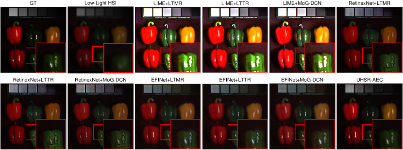
Fig. 3: Reconstructed images of various methods for the fake_and_real_peppers_ms (CAVE) dataset are illustrated by the false color image of [30,15,10] bands in Case 1.

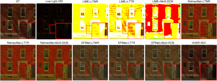
Fig. 4: Reconstructed images of various methods for the Imge3 (Harvard) dataset are illustrated by the false color image of [30,15,10] bands in Case 2.

4 Experiments

4.1 Experimental settings

Datasets: The datasets CAVE and Harvard are used to evaluate the effectiveness of the proposed method. The CAVE dataset contains 32 HSIs, each with 31 spectral bands and 512$\times$512 pixels, and we select 20 HSIs as the training dataset and 12 HSIs as the test dataset; the Harvard dataset contains 50 HSIs, each with 31 spectral bands and 1392$\times$1040 pixels, and we select 30 HSIs as the training dataset and 20 HSIs as the test dataset. Due to the limited computational resources, we crop and downsample each training HSI into 64$\times$64 pixels and each testing HSI into 256$\times$256 pixels.
Comparison methods and evaluation indicators: Peer methods compared with the proposed UHSR-AEC include three LLIE methods: LIME [19], RetinexNet [16], and EFINet [20]; and three HSI-SR methods: LTMR [12], LTTR [21], and MoG-DCN [22]. For consistency, the deep learning-based methods are all trained with the same HSI datasets.

In the experiments, all the HSI data are normalized to [0,1]. Four metrics are chosen to evaluate reconstructed HSI-SR image quality: peak signal-to-noise ratio (PSNR), structural similarity index (SSIM), spectral angle mapper (SAM), and the dimensionless global relative error of synthesis (ERGAS). All the experiments are performed on a server with a GPU NVIDIA 4090 graphics card.
Implementation Details: For each reference image, i.e., HR-HSI $\mathbf{Z}$ (GT), we adjust the image exposure by two different values of Gamma correction ($\alpha\in U(0.2,2)$, $\gamma\in U(0.5,3)$), for generating $\hat{\mathbf{Z}}_{x}$ and $\hat{\mathbf{Z}}_{y}$; the observation $\mathbf{X}$ is generated from $\hat{\mathbf{Z}}_{x}$ via Gaussian blurring (Gaussian kernel size of 8, mean of 0, standard deviation of $\sqrt{3}$) and downsampling (downsampling ratio of $K=|\mathbf{Z}|/|\mathbf{X}|=4$); the observation $\mathbf{Y}$ is generated through the convolutional integration of $\hat{\mathbf{Z}}_{y}$ with a real simulated spectral response (based on a Nikon camera).

We use the Pytorch framework to implement the proposed method. In the proposed UHSR-AEC network, we use a four-layer Unet structure and the Adam optimizer with the learning rate $l_{r}=10^{-4}$, as well as the maximum number of iterations $I_{max}=250,000$. Moreover, $\beta_{1},\beta_{2},\beta_{3},\lambda,\eta_{1},\eta_{2},T$ are set to 0.001, 0.001, 0.005, 0.5, 0.3, 0.1, 3, respectively. We would like to mention that the loss functions in (6) and (7) are for one HSI training sample $(\hat{\bf Z},\hat{\bf Z}_{x},\hat{\bf Z}_{y})$, while for the case of multiple HSI training samples in our experiment, they are simply replaced by the sum of the corresponding loss functions associated with each sample [22].

4.2 Comparison with competitive methods

The simulation HSI and MSI data are generated using CAVE and Harvard datasets for the following two exposure degradation cases:

Case 1: ($\alpha_{1}$ = 0.5,$\gamma_{1}$ = 0.7) for HSI, and ($\alpha_{2}$ = 1.3,$\gamma_{2}$ = 1.5) for MSI.

Case 2: ($\alpha_{1}$ = 0.5,$\gamma_{1}$ = 2.0) for HSI, and ($\alpha_{2}$ = 0.8,$\gamma_{2}$ = 1.5) for MSI.

The obtained simulation results are shown in Table 1. As can be seen from this table, UHSR-AEC is overall superior to the other nine methods. For the visual quality assessment, Figs. 3 and 4 show some results for all tested methods on the CAVE and Harvard datasets, respectively. For each sub-image, the reconstructed HR-HSI for three spectral bands ([30,15,10]) is shown. From these sub-images, it can be observed that: i) LIME-based methods yield overly bright images, ii) RetinexNet and EFINet-based methods expose some detail loss and colour imbalance in Case 1 and Case 2, respectively, iii) UHSR-AEC shows the best visualization in both Case 1 and Case 2.

4.3 Ablation studies

Some results for Ablation experiments on the proposed UHSR-AEC are shown in Table 2, which are obtained using the CAVE dataset with exposure degradation parameters used in Case 1. One can see from this table, that the proposed UHSR-AEC performs worst without IM, while it (with IM) performs best only in terms of PSNR for $T=3$, and best for $T=4$ otherwise, indicating that IM is essential and a suitable value of $T$ is also needed for the proposed UHSR-AEC to operate in good shape.

5 Conclusion

We have presented a novel UHSR-AEC network for HSI-SR (as shown in Fig. 2), with the given HSI and MSI acquired under different exposures. The proposed UHSR-AEC, with the structure for deep unfolding for intelligent image fusion and IM for preserving image texture and details, is devised from a new degradation-restoration perspective, instead of two independent domains (i.e., LLIE and restoration) considered by most existing approaches. Extensive experiments are provided to demonstrate the superior overall performance of the proposed UHSR-AEC over some existing LLIE-SR based benchmark methods.

Table 2: UHSR-AEC ablation experimental results for performance sensitivity to IM module and system parameter $T$.

Methods	PSNR$\uparrow$	SSIM$\uparrow$	SAM$\downarrow$	ERGAS$\downarrow$
UHSR-AEC ($T$=3)	27.1015	0.8601	9.4557	11.0631
UHSR-AEC ($T$=2)	26.5207	0.8484	10.1317	11.7043
UHSR-AEC ($T$=4)	26.9205	0.8827	9.0812	10.7911
UHSR-AEC w/o IM ($T$=3)	22.6863	0.7259	12.4081	17.2980

References

- [1] Robert O Green, Michael L Eastwood, Charles M Sarture, Thomas G Chrien, Mikael Aronsson, Bruce J Chippendale, Jessica A Faust, Betina E Pavri, Christopher J Chovit, Manuel Solis, et al., “Imaging spectroscopy and the airborne visible/infrared imaging spectrometer (AVIRIS),” RSE, vol. 65, no. 3, pp. 227–248, 1998.
- [2] Yuan Xie, Yanyun Qu, Dacheng Tao, Weiwei Wu, Qiangqiang Yuan, and Wensheng Zhang, “Hyperspectral image restoration via iteratively regularized weighted Schatten -norm minimization,” IEEE TGRS, vol. 54, no. 8, pp. 4642–4659, 2016.
- [3] Hsuan Ren and Chein-I Chang, “Automatic spectral target recognition in hyperspectral imagery,” IEEE TAES, vol. 39, no. 4, pp. 1232–1249, 2003.
- [4] Zhang Ting-ting and Liu Fei, “Application of hyperspectral remote sensing in mineral identification and mapping,” in IEEE ICCSNT, 2012, pp. 103–106.
- [5] Renwei Dian, Leyuan Fang, and Shutao Li, “Hyperspectral image super-resolution via non-local sparse tensor factorization,” in IEEE CVPR, 2017, pp. 5344–5353.
- [6] Qi Wei, José Bioucas-Dias, Nicolas Dobigeon, Jean-Yves Tourneret, Marcus Chen, and Simon Godsill, “Multiband image fusion based on spectral unmixing,” IEEE TGRS, vol. 54, no. 12, pp. 7236–7249, 2016.
- [7] Xuelong Li, Guanlin Li, and Bin Zhao, “Low-light hyperspectral image enhancement,” IEEE TGRS, vol. 60, pp. 1–13, 2022.
- [8] Qi Xie, Minghao Zhou, Qian Zhao, Zongben Xu, and Deyu Meng, “MHF-Net: An interpretable deep network for multispectral and hyperspectral image fusion,” IEEE TPAMI, vol. 44, no. 3, pp. 1457–1473, 2020.
- [9] Quan Liu, Yiqun Ji, Jianhong Wu, and Weimin Shen, “Study on convex grating in hyperspectral imaging spectrometers,” in MIPPR, 2009, vol. 7494, pp. 158–164.
- [10] Naoto Yokoya, Takehisa Yairi, and Akira Iwasaki, “Coupled nonnegative matrix factorization unmixing for hyperspectral and multispectral data fusion,” IEEE TGRS, vol. 50, no. 2, pp. 528–537, 2011.
- [11] Weisheng Dong, Fazuo Fu, Guangming Shi, Xun Cao, Jinjian Wu, Guangyu Li, and Xin Li, “Hyperspectral image super-resolution via non-negative structured sparse representation,” IEEE TIP, vol. 25, no. 5, pp. 2337–2352, 2016.
- [12] Renwei Dian and Shutao Li, “Hyperspectral image super-resolution via subspace-based low tensor multi-rank regularization,” IEEE TIP, vol. 28, no. 10, pp. 5135–5146, 2019.
- [13] Lei Zhang, Jiangtao Nie, Wei Wei, Yong Li, and Yanning Zhang, “Deep blind hyperspectral image super-resolution,” IEEE TNNLS, vol. 32, no. 6, pp. 2388–2400, 2020.
- [14] Haidi Ibrahim and Nicholas Sia Pik Kong, “Brightness preserving dynamic histogram equalization for image contrast enhancement,” IEEE TCE, vol. 53, no. 4, pp. 1752–1758, 2007.
- [15] Daniel J Jobson, Zia-ur Rahman, and Glenn A Woodell, “Properties and performance of a center/surround retinex,” IEEE TIP, vol. 6, no. 3, pp. 451–462, 1997.
- [16] Wenhan Yang Jiaying Liu Chen Wei, Wenjing Wang, “Deep retinex decomposition for low-light enhancement,” in BMVC, 2018.
- [17] Wenhui Wu, Jian Weng, Pingping Zhang, Xu Wang, Wenhan Yang, and Jianmin Jiang, “Uretinex-net: Retinex-based deep unfolding network for low-light image enhancement,” in IEEE CVPR, 2022, pp. 5901–5910.
- [18] Yufei Wang, Yi Yu, Wenhan Yang, Lanqing Guo, Lap-Pui Chau, Alex C Kot, and Bihan Wen, “Exposurediffusion: Learning to expose for low-light image enhancement,” in IEEE CVPR, 2023, pp. 12438–12448.
- [19] Xiaojie Guo, Yu Li, and Haibin Ling, “LIME: Low-light image enhancement via illumination map estimation,” IEEE TIP, vol. 26, no. 2, pp. 982–993, 2016.
- [20] Chunxiao Liu, Fanding Wu, and Xun Wang, “EFINet: Restoration for Low-Light Images via Enhancement-Fusion Iterative Network,” IEEE TCSVT, vol. 32, no. 12, pp. 8486–8499, 2022.
- [21] Renwei Dian, Shutao Li, and Leyuan Fang, “Learning a low tensor-train rank representation for hyperspectral image super-resolution,” IEEE TNNLS, vol. 30, no. 9, pp. 2672–2683, 2019.
- [22] Weisheng Dong, Chen Zhou, Fangfang Wu, Jinjian Wu, Guangming Shi, and Xin Li, “Model-guided deep hyperspectral image super-resolution,” IEEE TIP, vol. 30, pp. 5754–5768, 2021.