Abstract

Following our previous studies on gravitational dark matter (GDM) production in the early Universe of preheating, we forecast high-frequency gravitational wave (GW) spectra as the indirect probe of such GDM. We use proper lattice simulations to handle the resonance, and to solve the GW equation of motion with resonance induced scalar field excitations as the source term. Our numerical results show that the Higgs scalar excitations in the Higgs preheating model give rise to magnitudes of GW energy density spectra of order $10^{-10}$ at frequencies $10-10^{3}$ MHz, whereas the inflaton fluctuation excitations in the inflaton self-resonant preheating model yield magnitudes of GW energy density spectrum up to $10^{-9}~{}(10^{-11})$ at frequencies near $30~{}(2)$ MHz for the index $n=4~{}(6)$.

1 Introduction

After the end of inflation the early Universe is believed to evolve with time in a manner such that the inflaton energy density is transferred to the radiation energy density. This corresponds to the equation of state from $w=0$ to $w=1/3$. No matter what the underlying dynamics is, it enables the early Universe to provide a circumstance where various hypothetical particles such as dark matter (DM) can be produced as well. Motivated by null results of experiments aiming to detect non-gravitational DM, in this work we focus on gravitational dark matter (GDM) that only interacts with other matters via gravitational portal, see [1] for a recent review.

GDM can be produced in the early Universe either in the circumstance of reheating [2, 3, 4, 5, 6, 7, 8, 9, 10, 11, 12, 13, 14, 15] or recently studied preheating [16, 17, 18, 19]. In the case of reheating, a perturbative “decay” of the parent inflaton condensate converts its energy density into the daughter Standard Model (SM) particles. In the case of preheating, this energy transfer is achieved via a resonant production of daughter fields, caused by oscillations of the parent inflaton condensate. While these studies have demonstrated that the observed DM relic abundance can be satisfied, it is rather challenging to test the GDM. The main reasons include (i) the GDM is absolutely stable, implying that indirect limits derived from DM decay are not viable for the GDM, and (ii) either the GDM annihilation, GDM self scattering, or the GDM scattering off SM particles are always Planck-scale suppressed, suggesting that the GDM is out of reaches of these experiments. Compared to these late-time probes, other probes of the early Universe seem more promising.

In this study we consider high-frequency gravitational waves (GWs) as the indirect probe of GDM. In the context of reheating, GWs are emitted by the perturbative decay induced daughter fields [20, 21, 22, 23, 24]. Likewise, in the context of preheating they are emitted by the resonance induced daughter fields [25, 26, 27, 28, 29, 30, 31, 32, 33, 34, 35, 36, 37]. Once created, they immediately decouple on the contrary to the Cosmic Microwave Background (CMB). This means that such GWs may be the only way to uncover information about the evolution of the early Universe. Following this intuition, we continue to explore the high-frequency GW spectra emitted alongside with the GDM production during preheating as we have previously studied in [18, 19].

The rest of the paper is organized as follows. Sec.2 addresses the GW production in the Higgs preheating. We firstly discuss the resonant excitations of Higgs field, then use the obtained results to derive the present-day GW energy density spectra. Sec.3 addresses the GW production in the minimal preheating. As in Sec.2 we firstly analyze the self-resonance induced inflaton fluctuation excitations, then apply them to derive the present-day GW energy density spectra. To this end, we use proper lattice simulation [38, 39, 40] to handle the resonant process in each preheating model, during which one clearly sees the correlation between the growth of GWs and the excitations of relevant daughter scalar field. In appendix.A, we present the evaluation of the emitted GW spectra from the end time of preheating to the present time. Finally, we conclude in Sec.4, where we briefly comment on the detection prospects.

Note: throughout the text $M_{P}=2.4\times 10^{18}$ GeV is the reduced Planck mass scale, the subscript “end” and “_∗” denote the end of inflation and of lattice simulation respectively, and the subscript “0” is the present value.

2 The Higgs preheating

The Higgs preheating is built upon the following Lagrangian

$${}\mathcal{L}=\frac{1}{2}\partial_{\mu}\phi\partial^{\mu}\phi+\left(D_{\mu}H\right)^{{\dagger}}D^{\mu}H-V(\phi)-\kappa\mid H\mid^{2}\phi^{2},$$ (1)

where $V(\phi)$ denotes the inflation potential and the last term represents the interaction between the inflaton $\phi$ and the SM Higgs doublet with $\kappa$ being the dimensionless coupling constant. In [18] we have specifically considered the $\alpha$-attractor T-model of inflation [41, 42] with

$${}V(\phi)=\lambda_{\phi}M_{P}^{4}\left[\sqrt{6}\tanh\left(\frac{\phi}{\sqrt{6}M_{P}}\right)\right]^{2}\rightarrow\frac{1}{2}m^{2}_{\phi}\phi^{2},$$ (2)

which is approximated by a quadratic mass term with $m_{\phi}=\sqrt{2\lambda_{\phi}}M_{P}$ in the field range of $\mid\phi\mid<<M_{P}$.

Ignoring the Higgs self-interaction, we place constraints on the model parameters in eq.(1) as follows. First, one uses the Planck 2018 data [43] to fix the value of $\lambda_{\phi}$ in eq.(2) as $\lambda_{\phi}\approx 2.05\times 10^{-11}$. Second, the coupling $\kappa$ is upper bounded by the flatness of inflation potential as $\kappa<\sqrt{\lambda_{\phi}}$ and lower bounded by the preheating condition as $\kappa>\kappa_{\rm{min}}$, with $\kappa_{\rm{min}}\approx 2.5\times 10^{-7}$ the minimal value of $\kappa$ required by the parameter resonance. So we are left with the single model parameter $\kappa$ constrained to be in the narrow range of

$${}\kappa\sim(3-13)\times 10^{-7}.$$ (3)

2.1 Lattice treatment on parameter resonance

We begin with the equations of motion for the inflaton condensate and the SM Higgs:

$$\left(\frac{d^{2}}{dt^{2}}+3H\frac{d}{dt}\right)\phi+\frac{\partial V(\phi)}{\partial\phi} = 0,$$

$$\left(\frac{d^{2}}{dt^{2}}-\frac{\nabla^{2}}{a^{2}}+3H\frac{d}{dt}+m^{2}_{h,\lambda}\right)h_{\lambda} = 0,$$ (4)

where $h_{\lambda}$ are the four real scalars in the Higgs doublet with $\lambda=1$-4, $H$ is the Hubble rate, $a$ is the scale factor, “$\nabla$” is derivative over space coordinates, and $m^{2}_{h,\lambda}\approx\kappa\phi^{2}$ is the effective mass squared varying with time due to the oscillation of $\phi$.

To understand the parameter resonance induced Higgs field excitations, we make use of lattice simulations. In a practical lattice simulation, it is more convenient to introduce the re-scaled field variables instead of those in eq.(2.1)

$$\tilde{h}_{\lambda}=\frac{h_{\lambda}}{\phi_{\rm{end}}}~{}~{}\rm{and}~{}~{}\tilde{\phi}=\frac{\phi}{\phi_{\rm{end}}},$$ (5)

where $\phi_{\rm{end}}$ is the initial value of inflaton field after inflation. With the initial conditions [18],

$$\rho_{\phi,\rm{end}}=7.1\times 10^{62}\rm{GeV}^{4},~{}~{}\rho_{H,\rm{end}}=0,~{}~{}\phi_{\rm{end}}=0.84~{}M_{P},$$ (6)

we solve eq.(2.1) in terms of publicly available lattice code CosmoLattice [38, 39], by adopting the lattice size $N=128^{3}$ and the minimal infrared cut-off $k_{IR}=1$ in the following discussions of this section.

The top panel of fig.1 presents the evolution of the inflaton’s volume average $\left<\tilde{\phi}\right>$ (in blue) and the Higgs variance $\left<\tilde{h}^{2}_{\lambda}\right>$ (in orange) as function of time (in units of $\omega_{*}=m_{\phi}$) for $\kappa=3\times 10^{-7}$ (left) and $\kappa=13\times 10^{-7}$ (right) respectively. In this panel it is clear to see two critical points. (i) After a few oscillations, whenever the inflaton condensate crosses the zero points, i.e, $\tilde{\phi}(t)\rightarrow 0$, the value of $\left<\tilde{h}^{2}_{\lambda}\right>$ rapidly grows, as the effective mass $m^{2}_{h,\lambda}$ in eq.(2.1) vanishes at these points. (ii) When the backreaction due to the Higgs field becomes strong, which corresponds to the time $\omega_{*}t=100~{}(150)$ for $\kappa=3~{}(13)\times 10^{7}$, the growth of the Higgs variance stops.

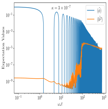
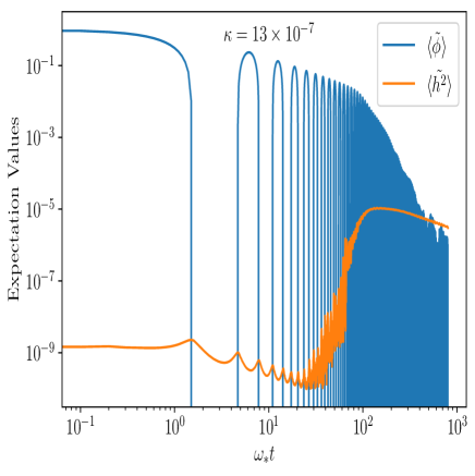
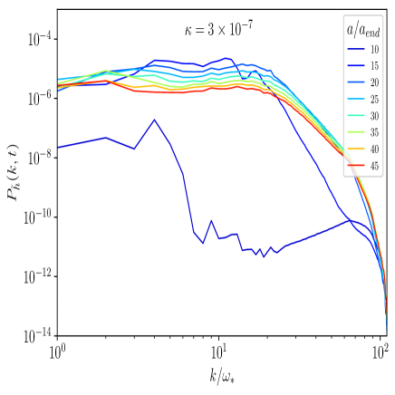
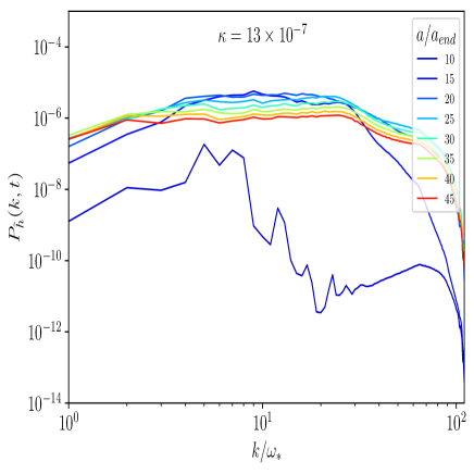
Figure 1: $\mathbf{Top}$: the evolution of inflaton’s volume average $\left<\tilde{\phi}\right>$ (in blue) and Higgs variance $\left<\tilde{h}^{2}_{\lambda}\right>$ (in orange) as function of time in units of $\omega_{*}$ for $\kappa=3\times 10^{-7}$ (left) and $\kappa=13\times 10^{-7}$ respectively. $\mathbf{Bottom}$: the evolution of Higgs power spectrum $P_{\tilde{h}}$ as function of $k$ with respect to time for $\kappa=3\times 10^{-7}$ (left) and $\kappa=13\times 10^{-7}$ respectively.

The bottom panel of fig.1 shows the evolution of Higgs power spectrum defined by

$$\left<\tilde{h}_{\lambda}(\mathbf{k})\tilde{h}^{*}_{\lambda}(\mathbf{k^{\prime}})\right>=(2\pi)^{3}P_{\tilde{h}_{\lambda}}(k)\delta(\mathbf{k}-\mathbf{k^{\prime}}),$$ (7)

with respect to time for $\kappa=3\times 10^{-7}$ (left) and $\kappa=13\times 10^{-7}$ (right) respectively, with the comoving wavenumber $k$ in units of $\omega_{*}$. Comparing the top and bottom panel, with the end of simulation time $a(t_{*})/a_{\rm{end}}=45$ in the later one corresponding to $\omega_{*}t_{*}\approx 720$ in the former one, one clearly sees that the growth of $P_{\tilde{h}_{\lambda}}(k)$ stops whenever the value of $\left<\tilde{h}^{2}_{\lambda}\right>$ gets stabilized. In addition, comparing the two red curves of $P_{\tilde{h}}$ in the bottom panel, one finds that as $\kappa$ increases, the value of $P_{\tilde{h}}$ increases in the large $k$ regime, but it becomes smaller in the small $k$ regime. This feature will help us understand the dependence of GW spectra on $\kappa$ as shown in fig.3.

2.2 Gravitational wave production

Having addressed the Higgs field excitations, we now derive the GWs produced during the resonant process. The GWs are determined by the equation of motion for the tensor perturbation $h_{ij}$ as

$$\ddot{h}_{ij}+3H\dot{h}_{ij}-\frac{\nabla^{2}}{a^{2}}h_{ij}=\frac{2}{M^{2}_{P}a^{2}}\Pi^{TT}_{ij},$$ (8)

where $\Pi^{TT}_{ij}=\Lambda_{ijk\ell}\Pi_{k\ell}$ is the transverse-traceless part of the effective anisotropic stress tensor, with

$$\Pi_{k\ell}=\partial_{k}\phi\partial_{\ell}\phi+\sum_{\lambda}\partial_{k}h_{\lambda}\partial_{\ell}h_{\lambda},$$ (9)

and $\Lambda_{ijk\ell}$ the projector. In terms of eq.(8) one obtains the produced GW energy density spectrum

$$\Omega_{\rm{GW}}(k,t)=\frac{1}{\rho_{c}}\frac{d\rho_{\rm{GW}}}{d\log k}(k,t)=\frac{k^{3}}{(4\pi)^{3}GV}\int\frac{d\Omega_{k}}{4\pi}\dot{h}_{ij}(\mathbf{k},t)\dot{h}^{*}_{ij}(\mathbf{k},t),$$ (10)

where $\rho_{c}$ is the total energy density during the preheating, $\Omega_{k}$ is the solid angle of Fourier space $\mathbf{k}$, and $V$ is the volume.

We use the lattice simulations developed in CosmoLattice [40] to solve a discrete version of eq.(8) in the Fourier space. Instead of projecting $\Pi$ to obtain $\Pi^{TT}$ and then solving $h_{ij}$ at every time step of evolution, this lattice code directly uses $\Pi$ to derive a tensor perturbation $u_{ij}$, then imposes the $\Lambda$ operator on $u_{ij}$ to obtain the physical $h_{ij}$. By doing so the consumption of simulation time is significantly reduced while the validity is guaranteed as both operations commute with each other. We refer the reader to [40] for more details about this point.

Fig.2 shows the GW energy density spectra in eq.(10) with respect to time for the two representative values of $\kappa=3\times 10^{-7}$ (left) and $\kappa=13\times 10^{-7}$ (right) respectively. We understand the evolution of the GW spectra by comparing fig.2 to the bottom panel of fig.1, where the time indices are the same. One finds that the time evolution of $\Omega_{\rm{GW}}(k)$ is correlated to that of $P_{\tilde{h}}(k)$, in the sense that the growth of the GW spectra almost immediately stops once the growth of $P_{\tilde{h}}(k)$ stops as shown by the red curves in these two figures. Such correlation between the resonance induced daughter field excitations and the daughter field induced GWs has also been verified by the study of another preheating in [36].

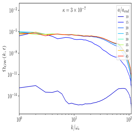
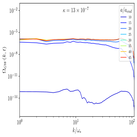
Figure 2: The Higgs excitations induced GW spectra with respect to time during the Higgs preheating for $\kappa=3\times 10^{-7}$ (left) and $\kappa=13\times 10^{-7}$ (right) respectively, where the time indices of the color curves are the same as in the bottom panel of fig.1.

In terms of the GW spectra at the end time of stimulation, with $a(t_{*})/a_{\rm{end}}=45$ as shown in fig.2, we show the present-day GW spectra $\Omega_{\rm{GW},0}(f)$ with respect to various values of $\kappa$ in the left panel of fig.3, by evaluating $\Omega_{\rm{GW}}(k,t_{*})$ from $t_{*}$ to the present time $t_{0}$ as shown in the appendix.A. In this figure the dependence of $\Omega_{\rm{GW},0}(f)$ on the model parameter $\kappa$ has been replaced by that of $\Omega_{\rm{GW},0}(f)$ on the GDM mass $m_{\chi}$, using the one-to-one correspondence between $\kappa$ and $m_{\chi}$ [18]. As $\kappa$ (alternatively $m_{\chi}$) increases, the magnitude of $\Omega_{\rm{GW},0}(f)$ is larger in the large $f$ regime, but it is smaller in the small $f$ regime, as previously seen in the dependence of $P_{\tilde{h}_{\lambda}}(k)$ on $\kappa$ in fig.1.

The emitted GWs can be understood as radiation, whose contribution to the effective neutrino number is determined by

$$\frac{7}{8}\left(\frac{4}{11}\right)^{4/3}\Delta N_{\rm{eff}}=\frac{\Omega^{\rm{tot}}_{\rm{GW},0}}{\Omega_{\rm{rad},0}},$$ (11)

where the total GW energy density

$$\Omega^{\rm{tot}}_{\rm{GW},0}=\int d\log k~{}\Omega_{\rm{GW}}(k,t_{0}).$$ (12)

Substituting the results of the left panel of fig.3 into eq.(11), one obtains the effective neutrino number as shown in the right panel of fig.3. Therein the values of $\Delta N_{\rm{eff}}$ range from $\sim 1\times 10^{-5}$ to $4\times 10^{-5}$, depending on the GDM mass $m_{\chi}$.

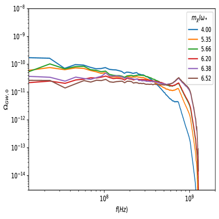
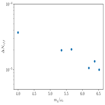
Figure 3: $\mathbf{Left}$: the present-day GW spectra with respect to various values of GDM mass $m_{\chi}$ using the one-to-one correspondence between $\kappa$ and $m_{\chi}$ [18]. $\mathbf{Right}$: the individual GW contribution to the effective neutrino number.

3 The minimal preheating

Unlike the Higgs preheating where the coupling of inflaton to the SM Higgs has to be introduced, the Lagrangian of the minimal preheating simply reads as

$${}\mathcal{L}=\frac{1}{2}\partial_{\mu}\phi\partial^{\mu}\phi-V(\phi)$$ (13)

where the inflation potential $V(\phi)$ is given by [41, 42]

$${}V(\phi)=\lambda_{\phi}M_{P}^{4}\left[\sqrt{6}\tanh\left(\frac{\phi}{\sqrt{6}M_{P}}\right)\right]^{n}\rightarrow\lambda_{\phi}\frac{\phi^{n}}{M^{n-4}_{P}},$$ (14)

with the index $n$ being an even number in order to make sure the positivity of the inflation potential. As explained in the beginning of Sec.2, the model parameter $\lambda_{\phi}$ has been fixed by the Planck data. Thus, $n$ is the only free parameter in eq.(13).

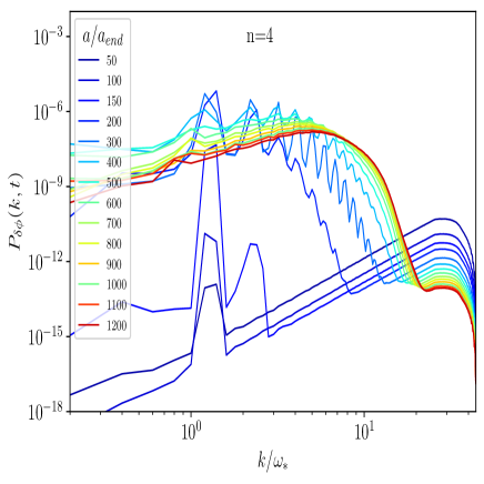
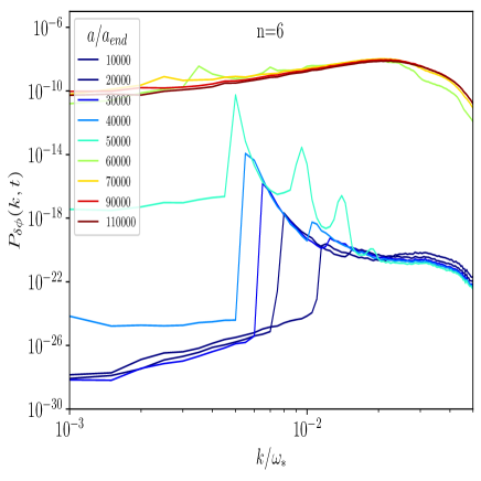
Figure 4: The evolution of the power spectrum $P_{\tilde{\delta\phi}}(k)$ with respect to time for $n=4$ (left) and $n=6$ (right) respectively, where $k$ is in units of $\omega_{*}$.

3.1 Lattice treatment on self-resonance

Similar to eq.(2.1) we start with the equations of motion for the inflaton condensate and its fluctuation $\delta\phi$:

$${}\ddot{\phi}+3H\dot{\phi}+\frac{\partial V}{\partial\phi} = 0,$$

$$\ddot{\delta\phi}+3H\dot{\delta\phi}-\frac{\nabla^{2}}{a^{2}}\delta\phi+\frac{\partial^{2}V}{\partial\phi^{2}}\delta\phi = 0.$$ (15)

Previously, the results of [44, 45, 46, 47] have shown that a self-resonant excitation of the inflaton fluctuations takes place for $n=4$ and 6, which has been verified by our recent work [19]. One can understand the self-resonance as a mixture of both parameter and tachyonic resonance by expanding the inflation field as $\phi(t)+\delta\phi(\mathbf{x},t)$ in eq.(14). In this sense, the analogy of the Higgs variance $\left<\tilde{\delta\phi}^{2}\right>$, with $\tilde{\delta\phi}=\delta\phi/\phi_{\rm{end}}$ defined as in eq.(5), is no longer suitable to illustrate the self-resonance. Rather, the analogy of Higgs power spectrum $P_{\tilde{\delta\phi}}(k)$ still works. Because the growth of $P_{\tilde{\delta\phi}}(k)$ is tied to that of GWs emitted by the inflaton fluctuation excitations.

Using the initial conditions displayed in Table 1 of [19] and adopting the lattice size $N=256^{3}~{}(128^{3})$ and the minimal infrared cut-off $k_{IR}=0.2~{}(5\times 10^{-4})$ for $n=4~{}(6)$ to solve eq.(3.1), we show the evolution of $P_{\tilde{\delta\phi}}(k)$ with respect to time in fig.4, with $k$ in units of $\omega_{*}$. The explicit values of $\omega_{*}$ can be found in [19]. Similar to the parameter resonance induced Higgs power spectrum $P_{\tilde{h}}(k)$ in Sec.2, the self-resonance induced power spectrum $P_{\tilde{\delta\phi}}(k)$ in this figure rapidly grows until the backreaction becomes strong. Afterward, it becomes stabilized as shown by the red curves with respect to $a(t_{*})/a_{\rm{end}}\approx 1.2\times 10^{3}~{}(1.1\times 10^{5})$ for $n=4~{}(6)$ respectively.

3.2 Gravitational wave production

Similar to eq.(8) the equation of motion for the tensor perturbation $h_{ij}$ during the minimal preheating is given by

$$\ddot{h}_{ij}+3H\dot{h}_{ij}-\frac{\nabla^{2}}{a^{2}}h_{ij}=\frac{2}{M^{2}_{P}a^{2}}\Pi^{TT}_{ij},$$ (16)

but with the effective anisotropic stress tensor

$$\Pi_{ij}=\partial_{i}\delta\phi\partial_{j}\delta\phi,$$ (17)

instead of eq.(9).

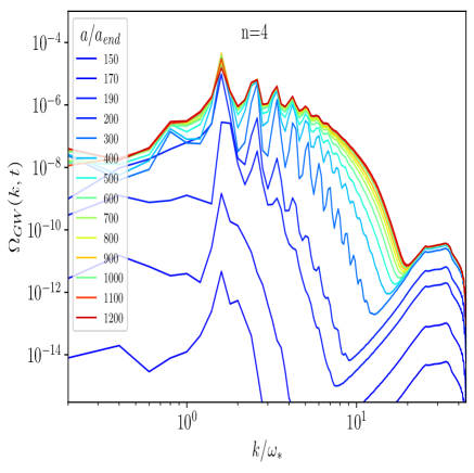
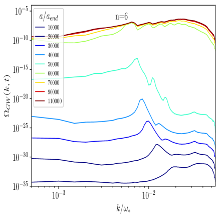
Figure 5: The inflaton fluctuation excitations induced GW spectra during the minimal preheating with respect to time for $n=4$ (left) and $n=6$ (right) respectively, where the time indices of the color curves are the same as in fig.4.

After solving the discrete version of eq.(16), we show in fig.5 the evolution of GWs produced during the minimal preheating with respect to time for $n=4$ (left) and $n=6$ (right) respectively, where the time indices of the color curves are the same as in fig.4. Similar to the correlation observed from figs.1 and 2 in the case of Higgs preheating, the growth of $\Omega_{\rm{GW}}(k)$ in fig.5 is correlated to that of $P_{\tilde{\delta\phi}}(k)$ in fig.4 as well in the case of minimal preheating either for $n=4$ or $n=6$. Fig.5 shows that there are multiple local peak frequencies in the $k$ regime of interest.These local peaks turn out to be imprinted in the present-day GW spectra as below.

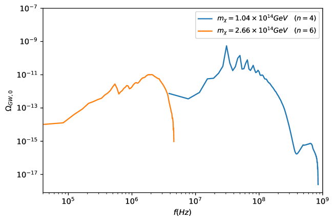
Figure 6: The present-day GW spectra with respect to the GDM mass $m_{\chi}=1.04~{}(2.66)\times 10^{14}$ GeV for $n=4~{}(6)$, using the one-to-one correspondence between $m_{\chi}$ and $n$ [19].

Using the results of fig.5 we show the present-day GW spectra in fig.6, by evaluating $\Omega_{\rm{GW}}(k)$ from the end time of preheating $t_{*}$ to the present time $t_{0}$ as shown in Appendix.A. In this figure several local peak frequencies previously seen in fig.5 appear near $\sim 40~{}(1)$ MHz for $n=4~{}(6)$. Moreover, the peak value of $\Omega_{\rm{GW},0}$ for $n=4$ is about two orders of magnitude larger than that for $n=6$, due to the relatively larger inflaton fluctuation excitations as illustrated by fig.4. Finally, consider the individual GW spectrum in fig.6 as radiation. It contributes to the effective neutrino number $\Delta N_{\rm{eff}}\approx 1.16\times 10^{-5}~{}(7.78\times 10^{-7})$ for $n=4~{}(6)$ after substituting the results of fig.6 into eq.(11).

4 Conclusion

In this work we have forecasted the GWs emitted alongside with the GDM production during the early Universe of preheating as the indirect probe of such GDM. Explicitly, we have considered two preheating models, where in the Higgs (minimal) preheating the GWs are emitted by the Higgs (inflaton fluctuation) excitations due to the parameter (self-) resonance. Our results have shown the distinct distributions of the emitted GW spectra in different high frequency ranges: (i) the Higgs scalar excitations in the Higgs preheating give rise to the magnitudes of GW energy density spectra of order $10^{-10}$ at frequencies $10-10^{3}$ MHz, and (ii) the inflaton fluctuation excitations in the minimal preheating yield the magnitudes of GW energy density spectrum up to $10^{-9}~{}(10^{-11})$ at frequencies near $30~{}(2)$ MHz for the index $n=4~{}(6)$.

While GWs at frequencies $10-10^{3}$ Hz have been detected by ground-based laser interferometers such as aLIGO [48] and GWs at frequencies $10^{-4}-1$ Hz are planned to be detected by space-based interferometers such as LISA [49], GW detectors at frequencies higher than $\sim$ MHz are lacking so far. Over the years several concepts [50] of high-frequency GW detectors have been proposed. Despite being out of sensitivity of the next-generation CMB measurements on $\Delta N_{\rm{eff}}$ [51], the above GW spectra could be in the reaches of some of these proposals in the near future.

There are a few points left for future study. First, GWs as the indirect probe of GDM from preheating can be also applied to the GDM from reheating, although in the later situation more diverse GW sources are expected. Second, the dependences of the GW spectra on the lattice size $N$ and cut-off $k_{IR}$ can be further suppressed by more powerful compute sources. Lastly, in order to eliminate the uncertainty in deriving the present-day GW spectra a more complete treatment on the equation of state between the end of preheating and of reheating than in the Appendix is needed.

Appendix A Evaluating gravitational wave spectrum

In this appendix we outline the evaluation of GW spectra from the end time of preheating $t_{*}$ to the present time $t_{0}$.

First, the present-day frequency $f$ is related to the physical wavenumber $k_{*}(a_{*}/a_{\rm{end}})^{-1}$ at the end of preheating as

$$f=\frac{1}{2\pi}\left(\frac{a_{*}}{a_{0}}\right)\left(\frac{k_{*}}{a_{*}/a_{\rm{end}}}\right)=\frac{1}{2\pi}\left(\frac{a_{*}}{a_{\rm{rad}}}\frac{a_{\rm{rad}}}{a_{0}}\right)\left(\frac{a_{\rm{end}}}{a_{*}}\right)k_{*},$$ (A.1)

where the ratios of scale factors in the first bracket can be written as

$$\frac{a_{*}}{a_{\rm{rad}}} = \epsilon^{1/4}_{*}\left(\frac{\rho_{\rm{rad}}}{\rho_{*}}\right)^{1/4}$$

$$\frac{a_{\rm{rad}}}{a_{0}} = G_{\rm{rad}}\left(\frac{\rho_{\rm{rad},0}}{\rho_{\rm{rad}}}\right)^{1/4},$$ (A.2)

with $\epsilon_{*}=(a_{*}/a_{\rm{rad}})^{1-3\bar{\omega}}$, $G_{\rm{rad}}=(g_{s,0}/g_{s,\rm{rad}})^{1/3}(g_{\rm{rad}}/g_{0})^{1/4}$ and $\rho_{*}\approx 3H^{2}_{*}M^{2}_{P}$. Here, $\bar{\omega}$ is the equation of state between the end of preheating and the onset of radiation domination, whereas $g_{s}$ and $g$ is the number of degrees of freedom associated with entropy and energy density respectively. Plugging eq.(A) into eq.(A.1) gives

$$f = \frac{1}{2\pi}\left(\frac{1}{3}\right)^{1/4}\epsilon^{1/4}_{*}G_{\rm{rad}}\rho^{1/4}_{\rm{rad},0}\left(\frac{a_{\rm{end}}}{a_{*}}\right)\left(\frac{H_{*}}{M_{P}}\right)^{1/2}\left(\frac{k_{*}}{H_{*}}\right),$$

$$\approx 5.5\times 10^{9}\left(\frac{a_{\rm{end}}}{a_{*}}\right)\left(\frac{H_{*}}{M_{P}}\right)^{1/2}\left(\frac{k_{*}}{H_{*}}\right)\rm{Hz},$$ (A.3)

where in the second line we have used $\epsilon_{*}\approx 1$ as $\bar{\omega}$ has been close to $1/3$ at the end of preheating, $G_{\rm{rad}}\approx 0.788$, and $\rho_{\rm{rad},0}\approx 3.37\times 10^{-51}$ GeV⁴.

Second, the present-day GW spectrum is related to that at the end of preheating as

$$\Omega_{\rm{GW},0}(f)=\frac{1}{\rho_{c,0}}\left(\frac{d\rho_{\rm{GW}}}{dk}\right)_{0}=\left(\frac{a_{*}}{a_{0}}\right)^{4}\frac{\rho_{*}}{\rho_{c,0}}\Omega_{\rm{GW},*}(k)$$ (A.4)

where $\rho_{c,0}$ is the present critical energy density and $\rho_{\rm{GW}}$ scales as $\sim a^{-4}$. Substituting the value of $a_{*}/a_{0}$ in terms of eq.(A) into eq.(A.4) one obtains

$$\Omega_{\rm{GW},0}(f) = \epsilon_{*}G^{4}_{\rm{rad}}\Omega_{\rm{rad},0}\Omega_{\rm{GW},*}(k),$$

$$\approx 2.0\times 10^{-5}\Omega_{\rm{GW},*}(k),$$ (A.5)

where $k_{*}$ is replaced by $f$ via eq.(A) and in the second line $\Omega_{\rm{rad},0}\approx 5\times 10^{-5}$ has been used. The main uncertainty in eq.(A) arises from $\epsilon_{*}$ which is sensitive to the value of $\bar{\omega}$.

References

- [1] E. W. Kolb and A. J. Long, [arXiv:2312.09042 [astro-ph.CO]].
- [2] T. Markkanen and S. Nurmi, JCAP 02, 008 (2017), [arXiv:1512.07288 [astro-ph.CO]].
- [3] M. Fairbairn, K. Kainulainen, T. Markkanen and S. Nurmi, JCAP 04, 005 (2019), [arXiv:1808.08236 [astro-ph.CO]].
- [4] S. Hashiba and J. Yokoyama, Phys. Rev. D 99, no.4, 043008 (2019), [arXiv:1812.10032 [hep-ph]].
- [5] Y. Ema, K. Nakayama and Y. Tang, JHEP 07, 060 (2019), [arXiv:1903.10973 [hep-ph]].
- [6] A. Ahmed, B. Grzadkowski and A. Socha, JHEP 08, 059 (2020), [arXiv:2005.01766 [hep-ph]].
- [7] E. Babichev, D. Gorbunov, S. Ramazanov and L. Reverberi, JCAP 09, 059 (2020), [arXiv:2006.02225 [hep-ph]].
- [8] Y. Mambrini and K. A. Olive, Phys. Rev. D 103, no.11, 115009 (2021), [arXiv:2102.06214 [hep-ph]].
- [9] B. Barman and N. Bernal, JCAP 06, 011 (2021), [arXiv:2104.10699 [hep-ph]].
- [10] S. Clery, Y. Mambrini, K. A. Olive and S. Verner, Phys. Rev. D 105, no.7, 075005 (2022), [arXiv:2112.15214 [hep-ph]].
- [11] B. Barman, S. Cléry, R. T. Co, Y. Mambrini and K. A. Olive, [arXiv:2210.05716 [hep-ph]].
- [12] O. Lebedev, T. Solomko and J. H. Yoon, [arXiv:2211.11773 [hep-ph]].
- [13] Y. Tang and Y. L. Wu, Phys. Lett. B 774, 676-681 (2017), [arXiv:1708.05138 [hep-ph]].
- [14] M. Garny, A. Palessandro, M. Sandora and M. S. Sloth, JCAP 02, 027 (2018), [arXiv:1709.09688 [hep-ph]].
- [15] M. Chianese, B. Fu and S. F. King, JCAP 06, 019 (2020), [arXiv:2003.07366 [hep-ph]].
- [16] A. Karam, M. Raidal and E. Tomberg, JCAP 03, 064 (2021), [arXiv:2007.03484 [astro-ph.CO]].
- [17] J. Klaric, A. Shkerin and G. Vacalis, JCAP 02, 034 (2023), [arXiv:2209.02668 [gr-qc]].
- [18] R. Zhang, Z. Xu and S. Zheng, JCAP 07, 048 (2023), JCAP 11, E01 (2023) (erratum), [arXiv:2305.02568 [hep-ph]].
- [19] R. Zhang and S. Zheng, JHEP 02, 061 (2024), [arXiv:2311.14273 [hep-ph]].
- [20] J. Garcia-Bellido, D. G. Figueroa and A. Sastre, Phys. Rev. D 77, 043517 (2008), [arXiv:0707.0839 [hep-ph]].
- [21] N. Bernal and F. Hajkarim, Phys. Rev. D 100, no.6, 063502 (2019), [arXiv:1905.10410 [astro-ph.CO]].
- [22] A. Ghoshal, L. Heurtier and A. Paul, JHEP 12, 105 (2022), [arXiv:2208.01670 [hep-ph]].
- [23] B. Barman, A. Ghoshal, B. Grzadkowski and A. Socha, JHEP 07, 231 (2023), [arXiv:2305.00027 [hep-ph]].
- [24] G. Choi, W. Ke and K. A. Olive, [arXiv:2402.04310 [hep-ph]].
- [25] S. Y. Khlebnikov and I. I. Tkachev, Phys. Rev. D 56, 653-660 (1997), [arXiv:hep-ph/9701423 [hep-ph]].
- [26] R. Easther, J. T. Giblin, Jr. and E. A. Lim, Phys. Rev. Lett. 99, 221301 (2007), [arXiv:astro-ph/0612294 [astro-ph]].
- [27] J. F. Dufaux, A. Bergman, G. N. Felder, L. Kofman and J. P. Uzan, Phys. Rev. D 76, 123517 (2007), [arXiv:0707.0875 [astro-ph]].
- [28] J. F. Dufaux, G. Felder, L. Kofman and O. Navros, JCAP 03, 001 (2009), [arXiv:0812.2917 [astro-ph]].
- [29] J. F. Dufaux, D. G. Figueroa and J. Garcia-Bellido, Phys. Rev. D 82, 083518 (2010), [arXiv:1006.0217 [astro-ph.CO]].
- [30] S. Y. Zhou, E. J. Copeland, R. Easther, H. Finkel, Z. G. Mou and P. M. Saffin, JHEP 10, 026 (2013), [arXiv:1304.6094 [astro-ph.CO]].
- [31] L. Bethke, D. G. Figueroa and A. Rajantie, JCAP 06, 047 (2014), [arXiv:1309.1148 [astro-ph.CO]].
- [32] P. Adshead, J. T. Giblin and Z. J. Weiner, Phys. Rev. D 98, no.4, 043525 (2018), [arXiv:1805.04550 [astro-ph.CO]].
- [33] K. D. Lozanov and M. A. Amin, Phys. Rev. D 99, no.12, 123504 (2019), [arXiv:1902.06736 [astro-ph.CO]].
- [34] D. G. Figueroa, A. Florio, N. Loayza and M. Pieroni, Phys. Rev. D 106, no.6, 063522 (2022), [arXiv:2202.05805 [astro-ph.CO]].
- [35] T. Krajewski and K. Turzyński, JCAP 10, 005 (2022), [arXiv:2204.12909 [astro-ph.CO]].
- [36] C. Cosme, D. G. Figueroa and N. Loayza, JCAP 05, 023 (2023), [arXiv:2206.14721 [astro-ph.CO]].
- [37] M. A. G. Garcia and M. Pierre, JCAP 11, 004 (2023), [arXiv:2306.08038 [hep-ph]].
- [38] D. G. Figueroa, A. Florio, F. Torrenti and W. Valkenburg, JCAP 04, 035 (2021), [arXiv:2006.15122 [astro-ph.CO]].
- [39] D. G. Figueroa, A. Florio, F. Torrenti and W. Valkenburg, [arXiv:2102.01031 [astro-ph.CO]].
-
[40]
“Cosmolattice: Gravitational Waves”,
https:
//cosmolattice.net/assets/technical_notes/CosmoLattice_TechnicalNote_GWs.pdf. - [41] R. Kallosh and A. Linde, JCAP 07, 002 (2013), [arXiv:1306.5220 [hep-th]].
- [42] R. Kallosh, A. Linde and D. Roest, JHEP 11, 198 (2013), [arXiv:1311.0472 [hep-th]].
- [43] Y. Akrami et al. [Planck], Astron. Astrophys. 641, A10 (2020), [arXiv:1807.06211 [astro-ph.CO]].
- [44] M. A. Amin, R. Easther and H. Finkel, JCAP 12, 001 (2010), [arXiv:1009.2505 [astro-ph.CO]].
- [45] M. A. Amin, R. Easther, H. Finkel, R. Flauger and M. P. Hertzberg, Phys. Rev. Lett. 108, 241302 (2012), [arXiv:1106.3335 [astro-ph.CO]].
- [46] K. D. Lozanov and M. A. Amin, Phys. Rev. Lett. 119, no.6, 061301 (2017), [arXiv:1608.01213 [astro-ph.CO]].
- [47] K. D. Lozanov and M. A. Amin, Phys. Rev. D 97, no.2, 023533 (2018), [arXiv:1710.06851 [astro-ph.CO]].
- [48] A. Buikema et al. [aLIGO], Phys. Rev. D 102, no.6, 062003 (2020), [arXiv:2008.01301 [astro-ph.IM]].
- [49] P. Auclair et al. [LISA Cosmology Working Group], Living Rev. Rel. 26, no.1, 5 (2023), [arXiv:2204.05434 [astro-ph.CO]].
- [50] N. Aggarwal, O. D. Aguiar, A. Bauswein, G. Cella, S. Clesse, A. M. Cruise, V. Domcke, D. G. Figueroa, A. Geraci and M. Goryachev, et al. Living Rev. Rel. 24, no.1, 4 (2021), [arXiv:2011.12414 [gr-qc]].
- [51] K. Abazajian, G. Addison, P. Adshead, Z. Ahmed, S. W. Allen, D. Alonso, M. Alvarez, A. Anderson, K. S. Arnold and C. Baccigalupi, et al. [arXiv:1907.04473 [astro-ph.IM]].