Imaginary-time relaxation quantum critical dynamics in two-dimensional dimerized Heisenberg model

Abstract

We study the imaginary-time relaxation critical dynamics of the Néel-paramagnetic quantum phase transition in the two-dimensional (2D) dimerized $S=1/2$ Heisenberg model. We focus on the scaling correction in the short-time region. A unified scaling form including both short-time and finite-size corrections is proposed. According to this full scaling form, improved short-imaginary-time scaling relations are obtained. We numerically verify the scaling form and the improved short-time scaling relations for different initial states using projector quantum Monte Carlo algorithm.

I Introduction

Quantum phase transitions (QPTs) describe nonanalytic changes between different ground states of many-body systems Sachdev (2011). Although QPTs are governed by quantum fluctuations at zero temperature, they can remarkably affect the finite-temperature phase diagram, giving rise to a variety of exotic behaviors in the famous quantum critical regime as exhibited in a wide range of strongly correlated systems Sachdev (2011); Sondhi et al. (1997). Thus the QPTs have received considerable attentions from both theoretical and experimental aspects. Among various models of QPTs, the $S=1/2$ Heisenberg antiferromagnet has attracted enormous investigations Chakravarty et al. (1988); Singh et al. (1988); Singh (1989); Millis and Monien (1993); Chubukov et al. (1994); Troyer et al. (1996); Kim and Troyer (1998); Matsumoto et al. (2001); Wang et al. (2006); Giamarchi et al. (2008); Sachdev (2008); Sandvik (2010); Merchant et al. (2014); Lohöfer et al. (2015); Wenzel et al. (2008); Qin et al. (2015); Ma et al. (2018); Wu et al. (2018); Tan et al. (2018); Tan and Jiang (2020); Sandvik and Scalapino (1994), not only because it is one of the typical quantum models whose ordered phase can spontaneously break continuous symmetry, but also owing to its close relation to strongly-correlated materials such as the cuprate superconductors Rønnow et al. (2001); Sachdev (2008); Manousakis (1991); Löhneysen et al. (2007).

Recent investigations on QPTs are increasingly focusing on their nonequilibrium dynamics, because the interplay between the divergent correlation time scale and the breaking of the translation symmetry in time direction can trigger lots of intriguing universal dynamic behaviors, which usually go beyond the conventional scheme of equilibrium QPTs Polkovnikov et al. (2011); Dziarmaga (2010); Stamper-Kurn and Ueda (2013); D’Alessio et al. (2016); Mitra (2018); Tsuji et al. (2013); Sieberer et al. (2013); Heyl et al. (2013); Jian et al. (2019); Yin and Jian (2021); Berges et al. (2021, 2004); Chiocchetta et al. (2015); Dağ et al. (2023); Marino et al. (2022); Li and Jian (2023). For example, in equilibrium, quantum criticality in $d$-dimension can usually be mapped into the corresponding classical criticality in $(d+1)$-dimension via the path-integral formulation Sachdev (2011); Sondhi et al. (1997). In contrast, for the nonequilibrium case, there is no similar mapping between quantum and classical critical dynamics. Besides the theoretical novelty, intriguing nonequilibrium critical phenomena have been found in various experiments Clark et al. (2016); Du et al. (2023); Navon et al. (2015); Lamporesi et al. (2013); Nicklas et al. (2015); Jurcevic et al. (2017). Moreover, quantum critical dynamics also has important applications in preparing and characterizing various exotic quantum phases in fast-developing quantum devices Weinberg et al. (2020); Dupont and Moore (2022); King et al. (2023); Semeghini et al. (2021); Ebadi et al. (2021).

Aside from the real-time dynamics, imaginary-time dynamics in quantum systems is also of great interest and significance. Because of its dissipative nature, the imaginary-time evolution usually works as a routine unbiased method to determine the ground state, not only widely used in numerical simulations, such as the time-evolving block decimation Vidal (2004, 2007), tensor network Jordan et al. (2008); Jiang et al. (2008), and quantum Monte Carlo (QMC) Sandvik (2010); Assaad and Evertz (2008); Li and Yao (2019), but also in rapidly developing quantum computers Motta et al. (2020); Nishi et al. (2021); Lin et al. (2021). Near a quantum critical point, it was shown that universal scaling behaviors appear not only in the long-time equilibrium stage, but also in short-time relaxation stage after a transient time scale Yin et al. (2014); Zhang et al. (2014). So far, the short-imaginary-time quantum critical dynamics has been studied in various quantum systems, including the quantum Ising model Yin et al. (2014); Zhang et al. (2014); Shu et al. (2017); Shu and Yin (2020), deconfined quantum criticality Shu et al. (2022); Shu and Yin (2022), and strongly-correlated Dirac systems Yu et al. (2023), providing an abundance of intriguing perspectives in the field of quantum criticality. In addition, the short-imaginary-time scaling behavior has been detected in an experimental platform of a noisy intermediate-scale quantum computer Zhang and Yin (2023). Moreover, the short-imaginary-time critical dynamics also shows its power in determining the critical properties with high efficiency, circumventing difficulties induced by critical slowing down and divergent entanglement entropy encountered in conventional methods based on equilibrium scaling Yin et al. (2014); Zhang et al. (2014); Shu et al. (2017); Shu and Yin (2020); Shu et al. (2022); Shu and Yin (2022); Yu et al. (2023); Zhang and Yin (2023). However, up to now, the short-imaginary-time scaling property has not been explored in the quantum Heisenberg universality class yet.

In this paper, we explore the imaginary-time relaxation critical dynamics of the Heisenberg universality class in the QPT between Néel antiferromagnetic (AFM) and quantum paramagnetic (PM) states in the two-dimensional dimerized Heisenberg model with inter- and intra-dimer couplings $J_{1}$ and $J_{2}$, as illustrated in Fig. 1. We find that the relaxation dynamics of this model exhibits scaling behaviors with remarkable short-time scaling corrections. A unified scaling form including both short-time and finite-size corrections is developed. From this scaling function, short-imaginary-time scaling properties with scaling correction included can be inferred. For different initial states, we find that the relaxation dynamics in the imaginary-time direction can be well described by this scaling form. The short-time scaling relations are also verified numerically. Our present work not only reveals the imaginary-time relaxation critical dynamics in the Heisenberg universality class, but also provides a systematic scaling analysis on the scaling corrections in the time direction, which be generalized to other kinds of nonequilibrium critical dynamics.

The rest of the paper is arranged as follows. The dimerized Heisenberg model is introduced in Sec. II. Then, in Sec. III, after a brief review on the original short-imaginary-time scaling theory in Sec. III.1, the scaling theory with short-time corrections is developed in Sec. III.2. The main numerical results are shown in Sec. IV. At last, a summary is given in Sec. V.

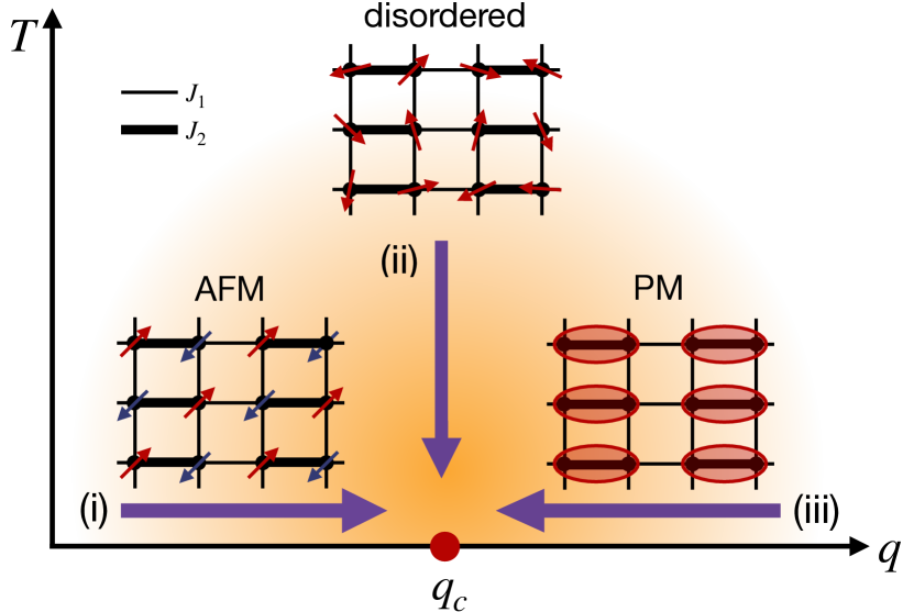
Figure 1: Sketch of the phase diagram and the quench protocol in imaginary-time with different initial states. $J_{1}$ and $J_{2}$ are the antiferromagnetic coupling on bonds $\langle ij\rangle$ (thin) and $\langle ij\rangle^{\prime}$ (thick), respectively. The initial states are prepared as (i) the Néel antiferromagnetic phase, (ii) the disordered state, and (iii) the dimerized paramagnetic state. All states correspond to the fixed points of the initial states under the renormalization group transformation.

II Model

The Hamiltonian of the $2$D dimerized Heisenberg model reads Chakravarty et al. (1988); Singh et al. (1988); Singh (1989); Millis and Monien (1993); Chubukov et al. (1994); Sachdev (2008)

$$H=J_{1}\sum_{\langle ij\rangle}\mathbf{S}_{i}\cdot\mathbf{S}_{j}+J_{2}\sum_{\langle ij\rangle^{\prime}}\mathbf{S}_{i}\cdot\mathbf{S}_{j},$$ (1)

in which $\mathbf{S}_{i}=(1/2)(\sigma_{x},\sigma_{y},\sigma_{z})$ denotes the spin-$1/2$ operator at site $i$, $J_{1}$ and $J_{2}$ are the antiferromagnetic coupling constants defined on the bonds $\langle ij\rangle$ and $\langle ij\rangle^{\prime}$, respectively, as illustrated in Fig. 1. When $q\equiv J_{2}/J_{1}\approx 1$, the ground state of Eq. (1) hosts the Néel AFM order Sandvik (2010); Ma et al. (2018), characterized by the order parameter ${\bf M}\equiv(1/L^{2})\sum_{r}(-1)^{r_{x}+r_{y}}\mathbf{S}_{r}$. In contrast, when $q>q_{c}=1.90951(5)$ Ma et al. (2018), the ground state changes to the paramagnetic (PM) state. It was shown that the dimerized Heisenberg model can be mapped to a nonlinear sigma model with an irrelevant Berry phase term and its criticality is well described by the Heisenberg $O(3)$ universality class Chakravarty et al. (1988); Chubukov et al. (1994); Sachdev (2008). This claim has been verified with scrutiny by numerical simulations via efficient quantum Monte Carlo methods Sandvik (2010).

III Scaling theory in short-imaginary-time quantum critical dynamics

In this section, after briefly reviewing the short-imaginary-time scaling theory in Sec. III.1, we generalize this theory to include the short-time and finite-size scaling corrections, as illuminated in Sec. III.2.

III.1 Brief review on short-imaginary-time quantum critical dynamics

The imaginary-time evolution of a quantum state $|\psi(\tau)\rangle$ is described by the imaginary-time Schrödinger equation

$$-\frac{\partial}{\partial\tau}|\psi(\tau)\rangle=H|\psi(\tau)\rangle,$$ (2)

imposed additionally by the normalization condition $\langle\psi(\tau)|\psi(\tau)\rangle=1$. Its formal solution is $|\psi(\tau)\rangle=Z\exp(-\tau H)|\psi(0)\rangle$, in which $|\psi(0)\rangle$ is the initial wave vector and $Z\equiv 1/\|\exp(-\tau H)|\psi(0)\rangle\|$ is the normalization factor. The expectation value of an operator $\mathcal{\hat{Q}}$ at $\tau$ is then given by

$$\mathcal{Q}(\tau)=\langle\psi(\tau)|\mathcal{\hat{Q}}|\psi(\tau)\rangle$$ (3)

For a gapped quantum system with an arbitrary initial state $|\psi(0)\rangle$, in which $|\psi(0)\rangle$ is assumed to have some overlap with the ground state, the wave function $|\psi(\tau)\rangle$, evolving according to Eq. (2), will fast decay to the ground state after a time scale $\tau_{\Delta}\sim 1/\Delta$ with $\Delta$ being the gap. Based on this, the imaginary-time evolution according to Eq. (2) provides an effective method to find the ground state numerically Vidal (2004, 2007); Jordan et al. (2008); Jiang et al. (2008); Sandvik (2010); Assaad and Evertz (2008); Li and Yao (2019). In contrast, when the system is at its critical point, $\Delta\rightarrow 0$ in the thermodynamics limit and thus $\tau_{\Delta}$ diverges. This reflects the critical slowing down in quantum phase transitions.

Associated with the divergence of $\tau_{\Delta}$, when the quantum system is near its critical point, nonequilibrium scaling behaviors appear in the imaginary-time relaxation process. It was shown that the scaling form of quantum imaginary-time dynamics is similar to that of classical short-time critical dynamics since both of them feature the dissipative nature Yin et al. (2014); Zhang et al. (2014); Janssen et al. (2014); Albano et al. (2011); Li et al. (1995); Zheng (1996). In the imaginary-time relaxation process, the general scaling form for an operator $\mathcal{Q}$ satisfies Yin et al. (2014); Zhang et al. (2014)

$$\mathcal{Q}(\tau,\delta,L,\{Y\})=\tau^{\kappa/z}f_{Q}(\delta\tau^{1/\nu z},\tau L^{-z},\{Y_{0}\tau^{-y_{0}/z}\}),$$ (4)

in which $\kappa$ is the critical exponent related to $\mathcal{Q}$, $\delta=q-q_{c}$ is the distance to the critical point and has a dimension of $1/\nu$ with $\nu$ being the correlation length exponent, $z$ is the dynamic exponent and ${Y_{0}}$ with its exponent $y_{0}$ denotes the relevant initial information. In the long-time limit, i.e., $\tau\gg L^{-z}$ and $\tau\gg|\delta|{-\nu}$, $Y_{0}$ vanishes and the usual equilibrium finite-size scaling form is recovered.

In particular, when the initial state corresponds to the fixed point of renormalization group transformation, such as the completely ordered and disordered initial states, the term of $Y_{0}$ can hide away in Eq. (4). In this way, the scaling form (4) becomes Yin et al. (2014); Zhang et al. (2014); Janssen et al. (2014); Albano et al. (2011); Li et al. (1995); Zheng (1996)

$$\mathcal{Q}(\tau,\delta,L)=\tau^{\kappa/z}f_{Q1}(\delta\tau^{1/\nu z},\tau L^{-z}).$$ (5)

Note that in this case the detailed function of $f_{Q1}$ still implicitly depends on $Y_{0}$. For example, from the completely ordered initial state, the evolution of the square of the order parameter, $M^{2}$, at $\delta=0$ satisfies Yin et al. (2014)

$$M^{2}(\tau,L)=\tau^{-2\beta/\nu z}f_{M1}(\tau L^{-z}),$$ (6)

in which $\beta$ is the order parameter exponent defined as $M\propto|\delta|^{\beta}$ in the ordered phase. In the short-time stage, $f_{M1}(\tau L^{-z})$ tends to a constant and

$$M^{2}\propto\tau^{-2\beta/\nu z},$$ (7)

whereas in the long-time stage, $f_{M1}(\tau L^{-z})\propto(\tau L^{-z})^{2\beta/\nu z}$ and scaling form restores to $M^{2}\propto L^{-2\beta/\nu}$ Sandvik (2010), which is the leading term of the finite-size scaling form

$$M^{2}(\tau,L)=L^{-2\beta/\nu}f_{M2}(\tau L^{-z}).$$ (8)

In addition, from the completely disordered initial state, $M^{2}$ obeys Albano et al. (2011); Shu et al. (2022)

$$M^{2}(\tau,L)=L^{-d}\tau^{-2\beta/\nu z+d/z}f_{M3}(\tau L^{-z}),$$ (9)

for $\delta=0$. In Eq. (9), $M^{2}\propto L^{-d}$ in the leading term comes from the the central limit theorem when the correlation length is smaller than $L$ Albano et al. (2011). In the short-time stage, $f_{M3}(\tau L^{-z})$ tends to a constant and

$$M^{2}\propto L^{-d}\tau^{-2\beta/\nu z+d/z},$$ (10)

whereas in the long-time stage, $f_{M3}(\tau L^{-z})\propto(\tau L^{-z})^{2\beta/\nu z-d/z}$, giving rise to $M^{2}\propto L^{-2\beta/\nu}$ and Eq. (8).

III.2 Scaling corrections in short-imaginary-time quantum critical dynamics

The above scaling analyses only consider the leading contributions of the relevant scaling variables. However, scaling corrections from the subleading contributions are also very important in describing quantum criticality. For example, it was shown that the finite-size scaling correction plays significant roles in determining critical properties for practical numerical simulations Sandvik (2010). Moreover, figuring out scaling corrections also provides strong evidences to clarify the universality classes of QPTs Sandvik (2010); Ma et al. (2018); Qin et al. (2015); Wenzel et al. (2008); Sushchyev and Wessel (2023). Previous investigations mainly focus on the scaling corrections from finite-size effects Sandvik (2010). For the nonequilibrium critical dynamics, the time is an intrinsic variable, such that the scaling correction from the time direction is quite essential and should be taken care carefully.

For simplicity, in the following, we shall consider the cases for which $\delta=0$ and initial states are at their fixed points under scale transformation. We start with the general scaling form of a quantity $\mathcal{Q}$

$$\mathcal{Q}(\tau,L)=L^{\kappa}f_{Q3}(\tau L^{-z},L^{-\omega_{L}},\tau^{-\omega_{\tau}}),$$ (11)

in which $L^{-\omega_{L}}$ is the usual finite-size scaling correction Sandvik (2010); Tan et al. (2018) and $\omega_{L}$ is the correction exponent, and $\tau^{-\omega_{\tau}}$ represents the short-time scaling corrections with $\omega_{\tau}$ the correction exponent. In Eq. (11), we assume that $\omega_{\tau}=\omega_{L}$ and both of them are denoted as $\omega$. This assumption is based on the fact that the critical theory of the quantum Heisenberg model has the Lorentz symmetry Chakravarty et al. (1988); Singh et al. (1988); Singh (1989); Millis and Monien (1993); Chubukov et al. (1994); Sachdev (2008) and will be verified by the numerical results in the next section.

However, directly using the full ansatz Eq. (11) is certainly unpractical since the detailed form of scaling function $f_{Q3}$ is unknown. Here, we propose that Eq. (11) can be approximated as

$$\mathcal{Q}(\tau,L)=L^{\kappa}(1+b_{Q}L^{-\omega})f_{Q4}[\tau L^{-z}(1+a_{Q}\tau^{-\omega})],$$ (12)

in which $b$ is the coefficient of finite-size correction and equals its equilibrium value, and $a$ is the coefficient of the short-time correction. Both $a$ and $b$ depend on the $\mathcal{Q}$. In addition, $a$ should also depend on the initial state.

The properties of Eq. (12) are discussed as follows. First, in the long-time limit, i.e., $\tau\rightarrow\infty$, $\tau^{-\omega}$ vanishes and $f_{Q4}(\tau L^{-z})$ tends to a constant. Accordingly, Eq. (12) is reduced to

$$\mathcal{Q}(\tau,L)\propto L^{\kappa}(1+b_{Q}L^{-\omega}),$$ (13)

which is consistent with the usual finite-size scaling relation with finite-size scaling correction included Sandvik (2010); Tan et al. (2018); Ma et al. (2018).

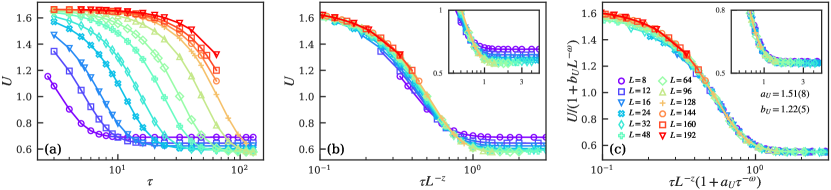
Figure 2: (a) Evolution of the Binder ratio from the completely ordered initial state for different lattice sizes at the critical point is shown. (b) When $\tau$ is rescaled as $\tau L^{-z}$, deviations still appear for the rescaled curves of $U$ versus $\tau$. (c) Rescaled curves collapse well when both short-time and finite-size scaling corrections are added. Note that in (c), the correction exponents for both time and size are set as $\omega=0.78$. Logarithmic scale is used in x-axis.

Second, to reveal the short-time scaling relations, we set $\tau L^{-z}(1+a_{Q}\tau^{-\omega})=c$, namely, $L=[\tau(1+a_{Q}\tau^{-\omega})/c]^{1/z}$. By substituting this equation into the leading term of Eq. (12), we obtain

$$\mathcal{Q}(\tau,L) = \tau^{\kappa/z}(1+a_{Q}\tau^{-\omega})^{\kappa/z}$$ (14)

$$\times (1+b_{Q}L^{-\omega})f_{Q5}[\tau L^{-z}(1+a_{Q}\tau^{-\omega})],$$

in which $c^{1/z}$ has been absorbed into $f_{Q5}$. From Eq. (14), one finds that for large $L$ in the short-time stage, the evolution of $\mathcal{Q}$ satisfies

$$\mathcal{Q}(\tau)\propto\tau^{\kappa/z}(1+a_{Q}\tau^{-\omega})^{\kappa/z}.$$ (15)

We will illustrate the short-imaginary-time scaling theory with scaling corrections for different quantities. For example, at the critical point $\delta=0$, with the initial state corresponding to its fixed point, the evolution of the dimensionless Binder cumulant, defined as $U\equiv\frac{5}{2}(1-\frac{5\langle M\rangle^{4}}{3\langle M^{2}\rangle^{2}}$), should satisfy

$$U(\tau,L)=(1+b_{U}L^{-\omega})f_{U}[\tau L^{-z}(1+a_{U}\tau^{-\omega})],$$ (16)

according to Eq. (12).

In addition, the square of the order parameter $M^{2}$ should obey

$$M^{2}(\tau,L)=L^{-2\beta/\nu}(1+b_{M}L^{-\omega})f_{M4}[\tau L^{-z}(1+a_{M}\tau^{-\omega})].$$ (17)

In particular, for an ordered initial state, the evolution of $M^{2}$ should follow the scaling form

$$M^{2}(\tau,L) = \tau^{-2\beta/\nu z}(1+a_{M}\tau^{-\omega})^{-2\beta/\nu z}$$ (18)

$$\times (1+b_{M}L^{-\omega})f_{M5}[\tau L^{-z}(1+a_{M}\tau^{-\omega})],$$

according to Eq. (14). Note that here the dependence of $a_{M}$ on the initial states is not explicitly shown to avoid complex labels. For large $L$, Eq. (18) indicates that in the short-time stage

$$M^{2}(\tau)\propto\tau^{-2\beta/\nu z}(1+a_{M}\tau^{-\omega})^{-2\beta/\nu z},$$ (19)

according to Eq. (15). Comparing with Eq. (7), one finds that a correction factor has been multiplied. In the next section, we will find that the factor is crucial in describing the short-imaginary-time relaxation dynamics of model (1).

Moreover, for a disordered initial state, $M^{2}$ should obey

$$M^{2}(\tau,L) = L^{-d}\tau^{-2\beta/\nu z+d/z}(1+a_{M}\tau^{-\omega})^{-2\beta/\nu z+d/z}$$ (20)

$$\times (1+b_{M}L^{-\omega})f_{M6}[\tau L^{-z}(1+a_{M}\tau^{-\omega})].$$

Note that the leading term of $L^{-d}$ is assumed to be not affected by the scaling correction, since $M^{2}(\tau,L)\propto L^{-d}$ is a direct result of the probability theory, rather than the result induced by the quantum fluctuations in QPT. For large $L$, Eq. (18) indicates that in the short-time stage

$$M^{2}(\tau,L)=L^{-d}\tau^{-2\beta/\nu z+d/z}(1+a_{M}\tau^{-\omega})^{-2\beta/\nu z+d/z},$$ (21)

according to Eq. (15). Compared with Eq. (10), again, a scaling correction factor is multiplied here.

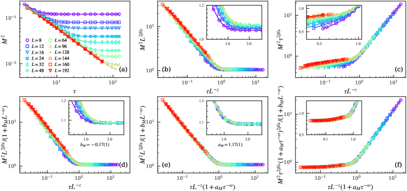
Figure 3: (a) Evolution of $M^{2}$ from the completely ordered AFM initial state for different lattice sizes at the critical point is plotted. Rescaled curves are shown in (b) and (c) according to Eqs. (8) and (6), respectively. Rescaled curves with only finite-size scaling corrections considered are shown in (d). Rescaled curves according to Eqs. (17) and (18), respectively, in which both short-time and finite-size scaling corrections are added. All insets address the details of the scaling collpase. Here both of $\beta/\nu=0.5185$ and $\omega=0.78$ Campostrini et al. (2002); Guida and Zinn-Justin (1998) are set as input. Double logarithmic scales are used.

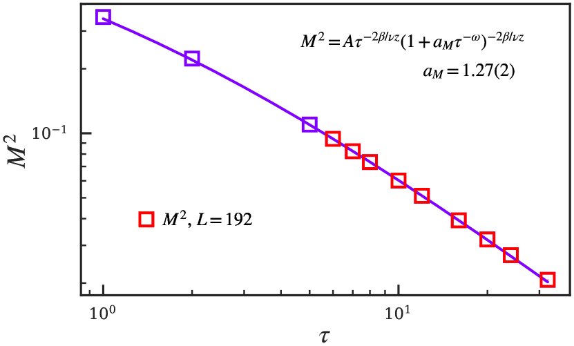
Figure 4: Dependence of $M^{2}$ on the evolution imaginary time $\tau$ with the ordered initial state for $L=192$ at the critical point. Power-law fitting according to Eq. (19) gives $a_{M}=1.27(2)$. Here both of $\beta/\nu=0.5185$ and $\omega=0.78$ Campostrini et al. (2002); Guida and Zinn-Justin (1998) are set as input. Double logarithmic scales are used.

IV Results

IV.1 Numerical method

We employ the projector QMC to implement the imaginary-time relaxation critical dynamics of model (1). We here briefly out line the method.

To realize the Schrödinger dynamics as introduced in Sec. III.1, in the projector QMC method, one takes the series expansion of the imaginary-time evolution operator $U(\tau)=\exp(-\tau H)$ in powers of $H^{n}$, and apply to the initial state $|\psi(0)\rangle$, giving $|\psi(\tau)\rangle=\sum_{n=0}^{\infty}\frac{\tau^{n}}{n!}(-H)^{n}|\psi(0)\rangle$. After splitting the Hamiltonian into bond operators and inserting unit operators into the operator sequence, the normalization $Z=\langle\psi(\tau)|\psi(\tau)\rangle$ can be importance sampled with the wave function written in a chosen basis, which is the standard spin-${z}$ basis or the valence-bond basis in this work, depending on the initial state desired. The actual expansion power $n$ is truncated to some maximum cut-off length that scales as $L^{d}\tau$ with vanishing truncation error. A full Monte Carlo sweep of the important sampling procedure consists of local diagonal updates and global off-diagonal updates, which updates the operator sequence and the basis states simultaneously. The local diagonal updates are carried out first, which replace unit operators with diagonal ones with appropriate acceptance rate and vice versa in the operator sequence. Then the global operator-loop updates follow up, which switch the operator types from diagonal to off-diagonal or vice versa and update the corresponding basis states. Detailed balance and ergodicity are maintained. The computational consumption of a full sweep of Monte Carlo update scales as $2\tau L^{d}$. The update schemes are mostly the same as those in the standard stochastic series expansion QMC method Sandvik (2010). Measurements are carried out in the middle of the double-sided projection, as indicated in Eq. (3). In studies of relaxation dynamics, the initial state of the system is crucial. It is important to note that in order to realize a given initial state, the imaginary-time boundaries are set fixed during the updates. In this work, three types of initial states are considered: (i) completely ordered AFM state, (ii) random disordered state, and (iii) dimerized PM state, as shown in Fig. 1. Types (i) and (ii) are implemented in the spin-$z$ basis while type (iii) employs the valence-bond basis so to maintain the dimerized order in the initial state. For a more detailed introduction of the method, we refer to the literature Sandvik (2010); Sandvik and Evertz (2010)

IV.2 AFM initial state

We first investigate the imaginary-time relaxation critical dynamics from the completely ordered AFM initial state.

The dynamics of the dimensionless Binder cumulant is shown in Fig. 2 (a). Figure 2 (b) shows that although rescaled curves of $U$ versus $\tau L^{-z}$ for different $L$ tends to collapse in comparison to Fig. 2 (a), apparent deviation remains for short-time and small-size cases. Then, we add the scaling corrections and rescale $U$ and $\tau$ according to Eq. (16). By tuning $a_{U}$ and $b_{U}$, we find the rescaled curves collapse very well, as shown in Fig. 2 (c). These results demonstrate the necessity of short-time and finite-size scaling corrections in the imaginary-time relaxation dynamics of model (1). In particular, in Fig. 2 (c), both the correction exponents $\omega_{\tau}$ and $\omega_{L}$ are chosen as $\omega=0.78$, which is analytically obtained in Ref. Guida and Zinn-Justin (1998) and numerically verified in Ref. Ma et al. (2018), confirming $\omega_{\tau}=\omega_{L}$ and the discussion below Eq. (11).

For the dynamic scaling behaviors of $M^{2}$, the evolution of $M^{2}$ for different system sizes is shown in Fig. 3 (a). By rescaling $M^{2}$ and $\tau$ as $M^{2}L^{2\beta/\nu}$ and $\tau L^{-z}$ according to Eq. (8), we find in Fig. 3 (b) that the rescaled curves in the short-time stage have apparent discrepancies although they tend to get close to each other. In particular, in the inset of Fig. 3 (b), one can find the discrepancy also occurs in the equilibrium region. In addition, Fig. 3 (c) shows that rescaled curves of $M^{2}\tau^{2\beta/\nu z}$ versus $\tau L^{-z}$ according to Eq. (6) also do not match with each other, in particular, for short-time and small-size regions. Moreover, in the short-time stage, Fig. 3 (c) shows that the rescaled curves are not parallel to the horizontal axis, even for large system size, demonstrating that the scaling relation of Eq. (7) does not give a complete description of the scaling behavior of $M^{2}$ in the short-time stage. Accordingly, scaling corrections are needed to improve the dynamic scaling theory discussed in Sec. III.1.

A natural question is whether these scaling discrepancies can be eliminated by usual finite-size scaling corrections. To examine it, in Fig. 3 (d), only the finite-size scaling correction is introduced. We find that for $b_{M}=-0.17(1)$ the rescaled curves match with each other quite well in the long-time stage, but they still deviate from each other in the short-time stage. Thus, an independent short-time scaling correction is required.

In Fig. 3 (e), both the short-time and finite-size scaling corrections are included according to Eq. (17). By tuning the coefficient before $\tau^{-\omega}$, $a_{M}$, but fixing the coefficient before $L^{-\omega}$, $b_{M}$, same as that in Fig. 3 (d), we find that for $a_{M}=1.17(1)$ the rescaled curves of $M^{2}L^{2\beta/\nu}$ versus $\tau L^{-z}$ can collapse quite well in the whole relaxation process.

In addition, by substituting the obtained $a_{M}$ and $b_{M}$ into Eq. (18) and rescaling the data according to this equation, we find that the rescaled curves also collapse quite well, as shown in Fig. 3 (f). These results not only successfully verify the effectiveness of scaling forms of Eqs. (17) and (18), but also determine the coefficient of the short-time scaling correction. Moreover, in Fig. 3 (f), the rescaled curves in the short-time stage are mainly parallel to the abscissa axis, demonstrating again that appropriate scaling corrections have been established.

To further reveal the short-time dynamic scaling behavior of $M^{2}$, in Fig. 4, we directly fit the curve of $M^{2}$ versus $\tau$ for large size $L=192$ according to Eq. (19) with the critical exponents set as input. We find that the prefactor before $\tau^{-\omega}$, $a_{M}$, determined from this fitting is $a_{M}=1.27(2)$, which is close to that obtained from data collapse in Fig. 3. Accordingly, we not only confirm that in the short-time stage, the evolution of $M^{2}$ satisfies Eq. (19), but also verify the value of $a_{M}$.

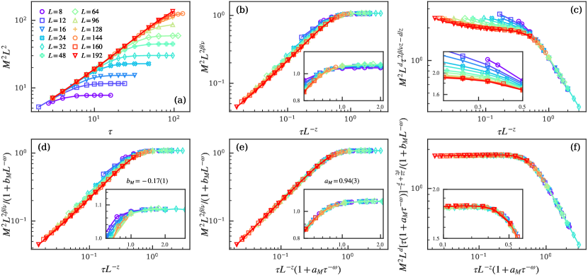
Figure 5: (a) Evolution of $M^{2}$ from the completely disordered initial state for different lattice sizes at the critical point is plotted. Rescaled curves are shown in (b) and (c) according to Eqs. (8) and (9), respectively. Rescaled curves with only finite-size scaling corrections considered are shown in (d). Rescaled curves according to Eqs. (17) and (20), respectively, in which both short-time and finite-size scaling corrections are added. All insets address the details of the scaling collpase. Here both of $\beta/\nu=0.5185$ and $\omega=0.78$ Campostrini et al. (2002); Guida and Zinn-Justin (1998) are set as input. Double logarithmic scales are used.

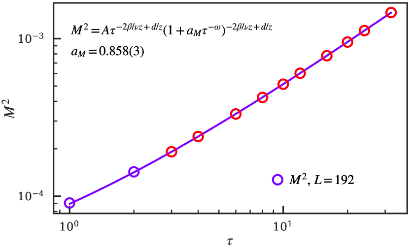
Figure 6: Dependence of $M^{2}$ on the evolution imaginary time $\tau$ with the disordered initial state for $L=192$ at the critical point. Power-law fitting according to Eq. (21) gives $a_{M}=0.858(3)$. Here both of $\beta/\nu=0.5185$ and $\omega=0.78$ Campostrini et al. (2002); Guida and Zinn-Justin (1998) are set as input. Double logarithmic scales are used.

IV.3 Disordered initial state

Next, we investigate the imaginary-time relaxation critical dynamics from the completely disordered initial state. This initial state can be regarded as the high-temperature thermal state, as illustrated in Fig. 1. We focus on the critical dynamics of $M^{2}$.

Figure 5 (a) shows the evolution of $M^{2}$ for different system sizes. Different from the decay feature for the ordered initial state, here, $M^{2}$ increases as $\tau$ increases. In addition, in the short-time stage, for large $L$, when the correlation length is smaller than the lattice size, $M^{2}\propto L^{-d}$. Thus, when plotting $M^{2}L^{d}$, we find that in the short-time and large-size region, the curves match with each other. This reflects that the relation of $M^{2}\propto L^{-d}$ does not need a scaling correction, since it is a direct result of the central limit theorem, as discussed in Sec. III.2.

We then rescale $M^{2}$ and $\tau$ for different system sizes according to the finite-size scaling form without scaling corrections, i.e., Eq. (8) and show the results in Fig. 5 (b). From Fig. 5 (b) and its inset, one finds that apparent separations appear in the short-time and small-size regions. The discrepancies in the short-time stage are more obvious when $M^{2}$ is rescaled according to Eq. (9), as shown in Fig. 5 (c). In addition, Fig. 5 (c) also sdemonstrates that in the short-time stage, the evolution of $M^{2}$ does not satisfy Eq. (10), since the rescaled curves are not parallel to the horizontal axis. Accordingly, scaling corrections are needed.

By including the finite-size scaling correction the same as the one in Fig 3, Fig. 5 (d) shows that this scaling correction can remedy the scaling mismatching in the long-time equilibrium stage. However the discrepancy still exists in the short-time stage.

These results inspire us to include both short-time and finite-size scaling corrections, similar to the previous case with an ordered initial state. In Fig. 5 (e), we rescale the curves of $M^{2}$ versus $\tau$ for different sizes according to Eq. (17), then tune the coefficient $a_{M}$ of the short-time correction term $\tau^{-\omega}$ with $b_{M}$ fixed as its equilibrium value, i.e., $b_{M}=-0.17(1)$. We find in Fig. 5 (e) that for $a_{M}=0.94(3)$, the rescaled curves for different sizes collapse quite well in the whole relaxation process, confirming the availability of Eq. (17). Besides, here the value of the prefactor $a_{M}$ is obviously different from the one for the ordered initial state, demonstrating that this coefficient depends on the initial state.

In addition, with the obtained $a_{M}$ and $b_{M}$, we rescale the data according to Eq. (20), we find that the rescaled curves also collapse quite well, as shown in Fig. 5 (f). These results successfully verify the effectiveness of the short-time scaling corrections in Eqs. (17) and (20). Moreover, as shown in Fig. 5 (f), the rescaled curves almost keep aclinic in the short-time stage, demonstrating again that appropriate scaling corrections have been introduced.

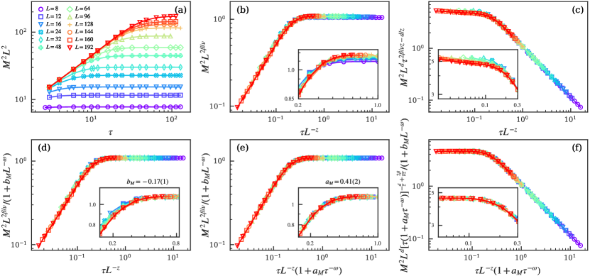
Figure 7: (a) Evolution of $M^{2}$ from the quantum PM initial state for different lattice sizes at the critical point is plotted. Rescaled curves are shown in (b) and (c) according to Eqs. (8) and (9), respectively. Rescaled curves with only finite-size scaling corrections considered are shown in (d). Rescaled curves according to Eqs. (17) and (20), respectively, in which both short-time and finite-size scaling corrections are added. All insets address the details of the scaling collpase. Here both of $\beta/\nu=0.5185$ and $\omega=0.78$ Campostrini et al. (2002); Guida and Zinn-Justin (1998) are set as input. Double logarithmic scales are used.

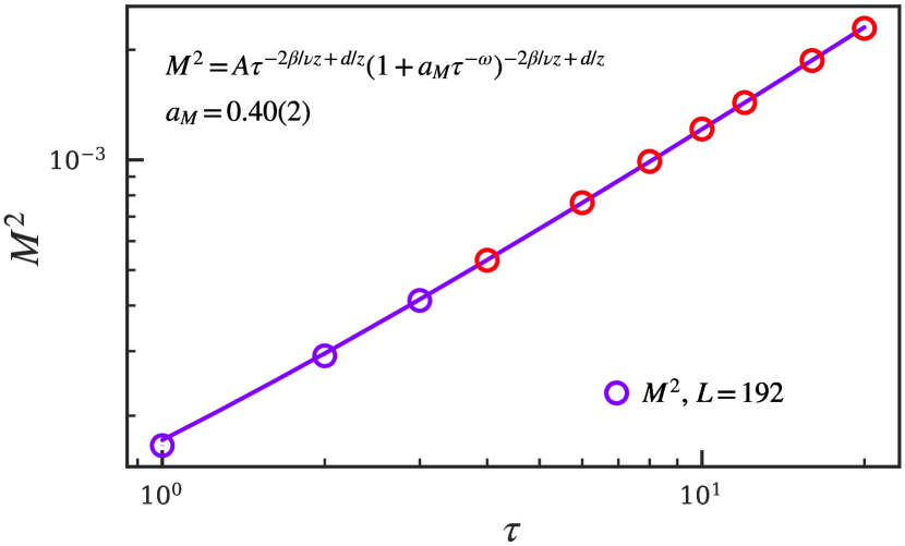
Figure 8: Dependence of $M^{2}$ on the evolution imaginary time $\tau$ with the PM initial state for $L=192$ at the critical point. Power-law fitting according to Eq. (21) gives $a_{M}=0.40(2)$. Here both of $\beta/\nu=0.5185$ and $\omega=0.78$ Campostrini et al. (2002); Guida and Zinn-Justin (1998) are set as input. Double logarithmic scales are used.

To further reveal the short-time dynamic scaling behavior of $M^{2}$, we directly fit the curve of $M^{2}$ versus $\tau$ for large size $L=192$ according to Eq. (21) with the critical exponents set as input. We find that the prefactor of the short-time correction obtained from this fitting is $a_{M}=0.858(3)$, close to that obtained from data collapse in Fig. 5. Accordingly, we not only show that in the short-time stage, the evolution of $M^{2}$ satisfies Eq. (21), but also confirm the value of the value of the coefficient of the short-time correction.

IV.4 Paramagnetic initial state

In this section, we turn to investigate the evolution of $M^{2}$ from the quantum PM initial state, as shown in Fig. 1. Although apparently different from the thermally disordered state, this PM state is also magnetically disordered with zero magnetization. Therefore, one expects similar scaling behaviors of $M^{2}$ to those in Sec. IV.3.

Figure 7 (a) shows the evolution of $M^{2}$ for different system sizes. Apparent discrepancies can be found in the rescaled curves when they are rescaled according to the scaling functions Eqs. (8) and (9) without scaling corrections, as shown in Figs. 7 (b) and (c). With only finite-size scaling correction included, Fig. 7 (d) shows that the discrepancy still exists in the short-time region.

Then, as shown in Figs. 7 (e) and (f), by rescaling the curves of $M^{2}$ versus $\tau$ for different sizes according to Eqs. (17) and (20), respectively, we find the rescaled curves for different sizes collapse well in the whole relaxation process when the prefactor $a_{M}$ in the short-time correction is chosen as $a_{M}=0.41(2)$. These results confirm the universality of the scaling forms of Eqs. (17) and (20). Moreover, as shown in Fig. 7 (f), the rescaled curves almost keep parallel to the horizontal axis in the short-time stage, demonstrating again that appropriate scaling corrections have been built.

The short-time dynamic scaling behavior of $M^{2}$ with the PM initial state is further explored in Fig. 8. Therein we directly fit the curve of $M^{2}$ versus $\tau$ for large size $L=192$ according to Eq. (21) with the critical exponents set as input. We find that the short-time correction prefactor is $a_{M}=0.40(2)$, close to that obtained from data collapse in Fig. 7. Accordingly, we not only show that in the short-time stage, the evolution of $M^{2}$ satisfies Eq. (20), but also confirm the value of $a_{M}$.

V Summary

In summary, we have studied the imaginary-time relaxation dynamics in the $2$D dimerized Heisenberg model. We have shown that remarkable discrepancies are found when the imaginary-time critical relaxation behaviors are described by the usual scaling forms. Moreover, we have found that besides the finite-size scaling correction, an additional short-time scaling correction is required to be included in the dynamic scaling theory. A full scaling form, including both short-time and finite-size scaling corrections, has been proposed. From this scaling form, modified short-imaginary-time relaxation scaling properties have been obtained. We have then verified these full scaling forms and short-time scaling properties for different initial states via QMC simulations. Note that the imaginary-time dynamics have been realized experimentally in the platforms of quantum computers to prepare the ground state of quantum systems Motta et al. (2020); Nishi et al. (2021); Lin et al. (2021). In particular, the short-imaginary-time scaling behavior is also been found in these systems Zhang and Yin (2023). Thus, it is expected that our results could be verified in the near-term quantum devices. Moreover, although the real-time dynamics have unitary nature, which is quite different from the dissipative nature of imaginary-time dynamics, both of real and imaginary time share the same scaling dimension Jian et al. (2019); Chiocchetta et al. (2015); Dağ et al. (2023); Marino et al. (2022); Li and Jian (2023). Therefore, it is expected that the real-time critical dynamics can have similar correction forms in time direction and this work is still in progress.

References

- Sachdev (2011) S. Sachdev, Quantum Phase Transitions, 2nd ed. (Cambridge Univ. Press, 2011).
- Sondhi et al. (1997) S. L. Sondhi, S. M. Girvin, J. P. Carini, and D. Shahar, Rev. Mod. Phys. 69, 315 (1997).
- Chakravarty et al. (1988) S. Chakravarty, B. I. Halperin, and D. R. Nelson, Phys. Rev. Lett. 60, 1057 (1988).
- Singh et al. (1988) R. R. P. Singh, M. P. Gelfand, and D. A. Huse, Phys. Rev. Lett. 61, 2484 (1988).
- Singh (1989) R. R. P. Singh, Phys. Rev. B 39, 9760 (1989).
- Millis and Monien (1993) A. J. Millis and H. Monien, Phys. Rev. Lett. 70, 2810 (1993).
- Chubukov et al. (1994) A. V. Chubukov, S. Sachdev, and J. Ye, Phys. Rev. B 49, 11919 (1994).
- Troyer et al. (1996) M. Troyer, H. Kontani, and K. Ueda, Phys. Rev. Lett. 76, 3822 (1996).
- Kim and Troyer (1998) J.-K. Kim and M. Troyer, Phys. Rev. Lett. 80, 2705 (1998).
- Matsumoto et al. (2001) M. Matsumoto, C. Yasuda, S. Todo, and H. Takayama, Phys. Rev. B 65, 014407 (2001).
- Wang et al. (2006) L. Wang, K. S. D. Beach, and A. W. Sandvik, Phys. Rev. B 73, 014431 (2006).
- Giamarchi et al. (2008) T. Giamarchi, C. Ruegg, and O. Tchernyshyov, Nature Physics 4, 198 (2008).
- Sachdev (2008) S. Sachdev, Nature Physics 4, 173 (2008).
- Sandvik (2010) A. W. Sandvik, AIP Conference Proceedings 1297, 135 (2010).
- Merchant et al. (2014) P. Merchant, B. Normand, K. W. Kramer, M. Boehm, D. F. McMorrow, and C. Ruegg, Nature Physics 10, 373 (2014).
- Lohöfer et al. (2015) M. Lohöfer, T. Coletta, D. G. Joshi, F. F. Assaad, M. Vojta, S. Wessel, and F. Mila, Phys. Rev. B 92, 245137 (2015).
- Wenzel et al. (2008) S. Wenzel, L. Bogacz, and W. Janke, Phys. Rev. Lett. 101, 127202 (2008).
- Qin et al. (2015) Y. Q. Qin, B. Normand, A. W. Sandvik, and Z. Y. Meng, Phys. Rev. B 92, 214401 (2015).
- Ma et al. (2018) N. Ma, P. Weinberg, H. Shao, W. Guo, D.-X. Yao, and A. W. Sandvik, Phys. Rev. Lett. 121, 117202 (2018).
- Wu et al. (2018) J. Wu, W. Yang, C. Wu, and Q. Si, Phys. Rev. B 97, 224405 (2018).
- Tan et al. (2018) D.-R. Tan, C.-D. Li, and F.-J. Jiang, Phys. Rev. B 97, 094405 (2018).
- Tan and Jiang (2020) D.-R. Tan and F.-J. Jiang, Phys. Rev. B 101, 054420 (2020).
- Sandvik and Scalapino (1994) A. W. Sandvik and D. J. Scalapino, Phys. Rev. Lett. 72, 2777 (1994).
- Rønnow et al. (2001) H. M. Rønnow, D. F. McMorrow, R. Coldea, A. Harrison, I. D. Youngson, T. G. Perring, G. Aeppli, O. Syljuåsen, K. Lefmann, and C. Rischel, Phys. Rev. Lett. 87, 037202 (2001).
- Manousakis (1991) E. Manousakis, Rev. Mod. Phys. 63, 1 (1991).
- Löhneysen et al. (2007) H. v. Löhneysen, A. Rosch, M. Vojta, and P. Wölfle, Rev. Mod. Phys. 79, 1015 (2007).
- Polkovnikov et al. (2011) A. Polkovnikov, K. Sengupta, A. Silva, and M. Vengalattore, Rev. Mod. Phys. 83, 863 (2011).
- Dziarmaga (2010) J. Dziarmaga, Advances in Physics 59, 1063 (2010).
- Stamper-Kurn and Ueda (2013) D. M. Stamper-Kurn and M. Ueda, Rev. Mod. Phys. 85, 1191 (2013).
- D’Alessio et al. (2016) L. D’Alessio, Y. Kafri, A. Polkovnikov, and M. Rigol, Advances in Physics 65, 239 (2016).
- Mitra (2018) A. Mitra, Annual Review of Condensed Matter Physics 9, 245 (2018).
- Tsuji et al. (2013) N. Tsuji, M. Eckstein, and P. Werner, Phys. Rev. Lett. 110, 136404 (2013).
- Sieberer et al. (2013) L. M. Sieberer, S. D. Huber, E. Altman, and S. Diehl, Phys. Rev. Lett. 110, 195301 (2013).
- Heyl et al. (2013) M. Heyl, A. Polkovnikov, and S. Kehrein, Phys. Rev. Lett. 110, 135704 (2013).
- Jian et al. (2019) S.-K. Jian, S. Yin, and B. Swingle, Phys. Rev. Lett. 123, 170606 (2019).
- Yin and Jian (2021) S. Yin and S.-K. Jian, Phys. Rev. B 103, 125116 (2021).
- Berges et al. (2021) J. Berges, M. P. Heller, A. Mazeliauskas, and R. Venugopalan, Rev. Mod. Phys. 93, 035003 (2021).
- Berges et al. (2004) J. Berges, S. Borsányi, and C. Wetterich, Phys. Rev. Lett. 93, 142002 (2004).
- Chiocchetta et al. (2015) A. Chiocchetta, M. Tavora, A. Gambassi, and A. Mitra, Phys. Rev. B 91, 220302 (2015).
- Dağ et al. (2023) C. B. Dağ, Y. Wang, P. Uhrich, X. Na, and J. C. Halimeh, Phys. Rev. B 107, L121113 (2023).
- Marino et al. (2022) J. Marino, M. Eckstein, M. S. Foster, and A. M. Rey, Reports on Progress in Physics 85, 116001 (2022).
- Li and Jian (2023) M.-R. Li and S.-K. Jian, arXiv: 2312.13531 (2023).
- Clark et al. (2016) L. W. Clark, L. Feng, and C. Chin, Science 354, 606 (2016), https://www.science.org/doi/pdf/10.1126/science.aaf9657 .
- Du et al. (2023) K. Du, X. Fang, C. Won, C. De, F.-T. Huang, W. Xu, H. You, F. J. Gómez-Ruiz, A. del Campo, and S.-W. Cheong, Nature Physics 19, 1495 (2023).
- Navon et al. (2015) N. Navon, A. L. Gaunt, R. P. Smith, and Z. Hadzibabic, Science 347, 167 (2015), https://www.science.org/doi/pdf/10.1126/science.1258676 .
- Lamporesi et al. (2013) G. Lamporesi, S. Donadello, S. Serafini, F. Dalfovo, and G. Ferrari, Nature Physics 9, 656 (2013).
- Nicklas et al. (2015) E. Nicklas, M. Karl, M. Höfer, A. Johnson, W. Muessel, H. Strobel, J. Tomkovič, T. Gasenzer, and M. K. Oberthaler, Phys. Rev. Lett. 115, 245301 (2015).
- Jurcevic et al. (2017) P. Jurcevic, H. Shen, P. Hauke, C. Maier, T. Brydges, C. Hempel, B. P. Lanyon, M. Heyl, R. Blatt, and C. F. Roos, Phys. Rev. Lett. 119, 080501 (2017).
- Weinberg et al. (2020) P. Weinberg, M. Tylutki, J. M. Rönkkö, J. Westerholm, J. A. Åström, P. Manninen, P. Törmä, and A. W. Sandvik, Phys. Rev. Lett. 124, 090502 (2020).
- Dupont and Moore (2022) M. Dupont and J. E. Moore, Phys. Rev. B 106, L041109 (2022).
- King et al. (2023) A. D. King, J. Raymond, T. Lanting, R. Harris, A. Zucca, F. Altomare, A. J. Berkley, K. Boothby, S. Ejtemaee, C. Enderud, E. Hoskinson, S. Huang, E. Ladizinsky, A. J. R. MacDonald, G. Marsden, R. Molavi, T. Oh, G. Poulin-Lamarre, M. Reis, C. Rich, Y. Sato, N. Tsai, M. Volkmann, J. D. Whittaker, J. Yao, A. W. Sandvik, and M. H. Amin, Nature 617, 61 (2023).
- Semeghini et al. (2021) G. Semeghini, H. Levine, A. Keesling, S. Ebadi, T. T. Wang, D. Bluvstein, R. Verresen, H. Pichler, M. Kalinowski, R. Samajdar, A. Omran, S. Sachdev, A. Vishwanath, M. Greiner, V. Vuleti, and M. D. Lukin, Science 374, 1242 (2021).
- Ebadi et al. (2021) S. Ebadi, T. T. Wang, H. Levine, A. Keesling, G. Semeghini, A. Omran, D. Bluvstein, R. Samajdar, H. Pichler, W. W. Ho, S. Choi, S. Sachdev, M. Greiner, V. Vuletić, and M. D. Lukin, Nature 595, 227 (2021).
- Vidal (2004) G. Vidal, Phys. Rev. Lett. 93, 040502 (2004).
- Vidal (2007) G. Vidal, Phys. Rev. Lett. 98, 070201 (2007).
- Jordan et al. (2008) J. Jordan, R. Orús, G. Vidal, F. Verstraete, and J. I. Cirac, Phys. Rev. Lett. 101, 250602 (2008).
- Jiang et al. (2008) H. C. Jiang, Z. Y. Weng, and T. Xiang, Phys. Rev. Lett. 101, 090603 (2008).
- Assaad and Evertz (2008) F. Assaad and H. Evertz, “World-line and determinantal quantum monte carlo methods for spins, phonons and electrons,” in Computational Many-Particle Physics, edited by H. Fehske, R. Schneider, and A. Weiße (Springer Berlin Heidelberg, Berlin, Heidelberg, 2008) pp. 277–356.
- Li and Yao (2019) Z.-X. Li and H. Yao, Annual Review of Condensed Matter Physics 10, 337 (2019), https://doi.org/10.1146/annurev-conmatphys-033117-054307 .
- Motta et al. (2020) M. Motta, C. Sun, A. T. K. Tan, M. J. O’Rourke, E. Ye, A. J. Minnich, F. G. S. L. Brandão, and G. K.-L. Chan, Nature Physics 16, 205 (2020).
- Nishi et al. (2021) H. Nishi, T. Kosugi, and Y.-i. Matsushita, npj Quantum Information 7, 85 (2021).
- Lin et al. (2021) S.-H. Lin, R. Dilip, A. G. Green, A. Smith, and F. Pollmann, PRX Quantum 2, 010342 (2021).
- Yin et al. (2014) S. Yin, P. Mai, and F. Zhong, Phys. Rev. B 89, 144115 (2014).
- Zhang et al. (2014) S. Zhang, S. Yin, and F. Zhong, Phys. Rev. E 90, 042104 (2014).
- Shu et al. (2017) Y.-R. Shu, S. Yin, and D.-X. Yao, Phys. Rev. B 96, 094304 (2017).
- Shu and Yin (2020) Y.-R. Shu and S. Yin, Phys. Rev. B 102, 104425 (2020).
- Shu et al. (2022) Y.-R. Shu, S.-K. Jian, and S. Yin, Phys. Rev. Lett. 128, 020601 (2022).
- Shu and Yin (2022) Y.-R. Shu and S. Yin, Phys. Rev. B 105, 104420 (2022).
- Yu et al. (2023) Y.-K. Yu, Z.-Zeng, Y.-R. Shu, Z.-X. Li, and S. Yin, arXiv: 2310.10601 (2023).
- Zhang and Yin (2023) S.-X. Zhang and S. Yin, “Universal imaginary-time critical dynamics on a quantum computer,” (2023), arXiv:2308.05408 [quant-ph] .
- Janssen et al. (2014) H. K. Janssen, B. Schaub, and B. Schmittmann, Zeitschrift für Physik B Condensed Matter 73, 539 (2014).
- Albano et al. (2011) E. V. Albano, M. A. Bab, G. Baglietto, R. A. Borzi, T. S. Grigera, E. S. Loscar, D. E. Rodriguez, M. L. R. Puzzo, and G. P. Saracco, Reports on Progress in Physics 74, 026501 (2011).
- Li et al. (1995) Z. B. Li, L. Schülke, and B. Zheng, Phys. Rev. Lett. 74, 3396 (1995).
- Zheng (1996) B. Zheng, Phys. Rev. Lett. 77, 679 (1996).
- Sushchyev and Wessel (2023) A. Sushchyev and S. Wessel, Phys. Rev. B 108, 235146 (2023).
- Campostrini et al. (2002) M. Campostrini, M. Hasenbusch, A. Pelissetto, P. Rossi, and E. Vicari, Phys. Rev. B 65, 144520 (2002).
- Guida and Zinn-Justin (1998) R. Guida and J. Zinn-Justin, Journal of Physics A: Mathematical and General 31, 8103 (1998).
- Sandvik and Evertz (2010) A. W. Sandvik and H. G. Evertz, Phys. Rev. B 82, 024407 (2010).