Hyperparameters in Continual Learning: a Reality Check

Abstract

Various algorithms for continual learning (CL) have been designed with the goal of effectively alleviating the trade-off between stability and plasticity during the CL process. To achieve this goal, tuning appropriate hyperparameters for each algorithm is essential. As an evaluation protocol, it has been common practice to train a CL algorithm using diverse hyperparameter values on a CL scenario constructed with a benchmark dataset. Subsequently, the best performance attained with the optimal hyperparameter value serves as the criterion for evaluating the CL algorithm. In this paper, we contend that this evaluation protocol is not only impractical but also incapable of effectively assessing the CL capability of a CL algorithm. Returning to the fundamental principles of model evaluation in machine learning, we propose an evaluation protocol that involves Hyperparameter Tuning and Evaluation phases. Those phases consist of different datasets but share the same CL scenario. In the Hyperparameter Tuning phase, each algorithm is iteratively trained with different hyperparameter values to find the optimal hyperparameter values. Subsequently, in the Evaluation phase, the optimal hyperparameter values is directly applied for training each algorithm, and their performance in the Evaluation phase serves as the criterion for evaluating them. Through experiments on CIFAR-100 and ImageNet-100 based on the proposed protocol in class-incremental learning, we not only observed that the existing evaluation method fail to properly assess the CL capability of each algorithm but also observe that some recently proposed state-of-the-art algorithms, which reported superior performance, actually exhibit inferior performance compared to the previous algorithm.

1 Introduction

In recent years, extensive research has been conducted on continual learning (CL) to effectively adapt to successive novel tasks while overcoming catastrophic forgetting for previous tasks [23]. However, a neural network in such CL scenarios faces a trade-off between achieving good performance on new tasks (plasticity) and maintaining knowledge on past tasks (stability) [15]. To address this inherent trade-off, numerous algorithms have been proposed. Especially, CL research in classification has attracted interests, primarily focusing on task-incremental learning [16, 7] among three scenarios of CL [20]. Notably, recent efforts have concentrated on class-incremental learning [14], recognized as the most challenging among them.

Various CL algorithms tailored for successful CL in classification offer novel approaches to balance stability and plasticity during the CL process. These algorithms can broadly be categorized into three groups [23, 16]: Regularization-based [12, 9, 18, 24], model expansion-based [25, 22, 21, 28], and exemplar-based methods [18, 24, 22, 28, 21, 9]. Despite differing approaches in these three categories, they inevitably require to introduce additional hyperparameters for their algorithm. Consequently, to apply these algorithms across diverse CL scenarios, tuning these hyperparameters becomes imperative. From an evaluation perspective, to assess these algorithms, most studies partition a benchmark dataset (e.g., CIFAR-100 [11] and ImageNet [8]) into multiple tasks, forming CL scenarios. Subsequently, they repetitively applied their algorithm to these scenarios with different hyperparameter values and reported the highest performance achieved with the optimal hyperparameter values [7, 23, 14].

Despite the ongoing reports on the success of newly developed state-of-the-art algorithms in achieving remarkable performance through the above hyperparameter tuning method [21, 22, 28], we contend that this evaluation protocol inherently poses specific challenges. Firstly, it results in overfitting of hyperparameters to the provided dataset and CL scenario, posing a challenge in assessing the algorithm’s CL capability. Secondly, From the perspective of real world applications, this current hyperparameter tuning method is unfeasible due to the impracticality of iteratively accessing the entire task dataset.

To address the limitations of the existing evaluation protocol, we revisit the fundamental principles of evaluation in machine learning. Namely, to assess the CL capability of each algorithm, we introduce an evaluation method utilizing the Hyperparameter Tuning and Evaluation phases. These phases share the same CL scenario but are composed of different datasets. Initially, in the Hyperparameter Tuning phase, where access to all task data is always available, models are trained with each CL algorithm using various hyperparameter values. Following this, we determine the best hyperparameter values, which yield superior performance for each algorithm. Subsequently, these optimal hyperparameter values are directly applied to train models with each algorithm in the Evaluation phase, and the performance in this phase serves as the benchmark for their evaluation. As the first application of the proposed protocol, we opted for state-of-the-art class-incremental learning (CIL) algorithms. From experiments with the CIFAR-100 and ImageNet-100 datasets, we obtained the following experimental findings:

• Firstly, the reported performance of most state-of-the-art CIL algorithms in the conventional evaluation protocol stems from overfitting of hyperparameters to a specific dataset or CL scenario. This indicates that the performance of these algorithms does not generalize effectively in our evaluation protocol.

• Secondly, in the case of current state-of-the-art algorithms based on the model expansion (e.g., FOSTER [22], BEEF [21] and MEMO [28]), it achieved relatively poorer performance compared to the older baseline (i.g., DER) in our evaluation protocol.

In conclusion, the hyperparameter tuning approach used in the conventional evaluation protocol is not only impractical but also fails to adequately evaluate the CL capability of each algorithm. This highlights the necessity of adopting the proposed protocol for a more comprehensive evaluation of CL algorithms.

2 Related Work

Continual learning   Continual learning (CL) research has evolved in various forms [23, 16, 7, 14]. Initially, CL studies focused on task-incremental learning (TIL) in image classification [16, 7], exploring diverse approaches such as regularization-based methods, which measure the importance of weights learned from previous tasks and overcome catastrophic forgetting through regularization [12, 1, 5, 2]. Additionally, model expansion-based methods, which partially freeze to address catastrophic forgetting and selectively expand the model during CL, have shown promising results [19, 26]. Subsequently, researchers shifted their attention to more challenging scenarios, particularly class-incremental learning (CIL) [14]. This shift led to the investigation of exemplar-based methods, involving the effective utilization of exemplar memory storing a subset of previous tasks’ datasets [18]. Additionally, algorithms, that combine the exemplar-based method with the regularization-based method, show notable performance achievements [24, 9, 27, 3]. Recently, combining the exemplar-based method with the model expansion-based method has been considered as the most powerful method, showing overwhelming performance [22, 25, 28, 21] in various CIL scenarios.

Evaluation and hyperparameter tuning of CL   For the appropriate evaluation of CL algorithms, discussions on an evaluation metric have taken various forms, encompassing fundamental metrics such as average and final accuracy. Initially, [5] proposed accuracy-based metrics to assess the stability and plasticity. While these accuracy-based metrics continue to be commonly used for evaluating CL algorithms, some studies have pointed out their limitations, in terms of their actual computational cost [17] and the quality of learned representations by them [4]. On the other hand, studies on hyperparameter tuning for offline CL algorithms have also been conducted. [16] proposed the grid search-based method for TIL, and [13] introduced the bandit algorithm-based approach for CIL. However, these algorithms not only demand additional training costs for applying their method for hyperparameter tuning but also focus solely on searching for the unique hyperparameters of each CL algorithm. In contrast, for online CL, an evaluation protocol considering hyperparameter tuning, similar to the one proposed in this paper, was suggested [6]. However, this protocol is yet to be widely considered as standard in online CL and is rarely explored in the context of offline CL until now.

3 Proposed Evaluation Protocol

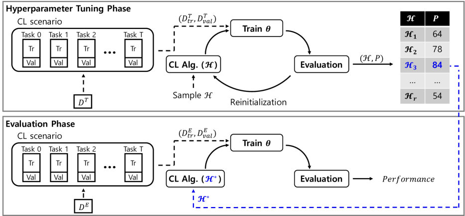
Figure 1: Illustration of the proposed two phases. Note that both phases share the same CL scenario, but the two datasets ($D^{T}$ and $D^{E}$) are distinct from each other. In experiments, to comprehensively assess the CL capability of each algorithm, we explore two scenarios where the datasets exhibit either high or low similarity.

3.1 Motivation: Hyperparameter tuning of CL

To gauge the continual learning (CL) capability of each algorithm, several studies have conducted assessments using benchmark datasets, including CIFAR-100 and ImageNet, within various predefined CL scenarios (e.g., sequentially learning 10 tasks, each comprised of 10 classes) [16, 7, 23]. In the realm of CL research in image classification, the primary evaluation metric has been based on classification accuracy on validation data. For example, in the challenging realm of class-incremental learning (CIL), accuracy on the entire validation dataset after learning the last task emerged as a crucial metric [14]. Supplementary metrics, such as stability and plasticity, based on validation accuracy for each task, have been employed to further demonstrate algorithmic proficiency [5, 14]. Despite ongoing skepticism regarding the effectiveness of accuracy-based evaluation methods [4, 17], they remain pivotal in distinguishing state-of-the-art algorithm until now.

In light of this, we cast doubt on the effectiveness of the current evaluation protocol in accurately assessing the CL ability of each algorithm. Specifically, we question the practice of configuring CL scenarios using training and validation data from benchmark datasets and then tuning hyperparameters for each algorithm directly. This protocol involves identifying optimal hyperparameter values that maximize validation accuracy for the given CL scenario and presenting this performance as the major evaluation criterion. For instance, as illustrated in the top figure in Figure 1, the evaluation criterion for the given CL algorithm becomes 84% of accuracy for $\mathcal{H}_{3}$. In this regards, it is crucial to note that this evaluation protocol encounters two major challenges. Firstly, evaluating each algorithm in this manner results in performance influenced by hyperparameters values tuned specifically to the provided dataset and CL scenario, raising concerns about the generalizability of their CL capability. Secondly, choosing the optimal hyperparameter values for each algorithm by reproducing this hyperparameter tuning process in real world scenarios is impractical. This is due to the uncertainty of future tasks and the challenge of executing an identical CL scenario repeatedly.

3.2 Realistic evaluation protocol considering hyperparameters in continual learning

Given the challenges posed by the current evaluation protocol, a crucial question emerges: How can we effectively assess the CL capability of each algorithm? To tackle these challenges, we return to a fundamental machine learning evaluation principle and propose a two-phase approach: Hyperparameter Tuning and Evaluation phases. As illustrated in Figure 1 and Algorithm 1, the Hyperparameter Tuning phase is dedicated to finding optimal hyperparameter values for each algorithm, while the Evaluation phase assesses the CL capability using the identified optimal hyperparameter values in the same CL scenario generated from the different dataset. Note that both phases consist of different datasets (e.g., $D^{T}\neq D^{E}$), such as having a disjoint set of classes in CIL, while sharing the same CL scenario.

Algorithm 2 outlines the pseudo algorithm for the Hyperparameter Tuning phase. Initially, we randomly sample a hyperparameter value $h_{k}$ from the predefined set of values $h_{k}^{Set}$ to compose a list of selected hyperparameter values $\mathcal{H}_{r}$. Subsequently, we generate the predefined CL scenario using the function $\mathcal{F}$ with multiple class orderings obtained by shuffling. We then train a model $\theta$ using a CL algorithm $\mathcal{A}$, $\mathcal{H}_{r}$, and the training dataset $D^{T}_{tr}$, followed by evaluating the model’s performance ($P$) on the validation dataset $D^{T}_{val}$. This phase returns $R$ sets, each containing a list of hyperparameter values and the corresponding evaluation result. The subsequent step entails selecting the optimal hyperparameter values, denoted as $\mathcal{H}^{*}$, using the SelectBestSet function outlined in Algorithm 1. This function returns the hyperparameter values chosen based on a specific criterion. In the Evaluation phase, presented in Algorithm 3, we train a model $\theta$ using the CL algorithm with the best hyperparameter values $\mathcal{H}^{*}$ and the dataset $D^{E}_{tr}$. Finally, the averaged performance of the trained model over multiple class orderings becomes the criterion for evaluating the given CL algorithm $\mathcal{A}$.

Note that, while a similar method to the proposed protocol have been suggested and utilized in the online CL [6], many recent studies, particularly the majority of offline CL research, have not considered this evaluation protocol [23]. Additionally, the proposed evaluation protocol differs from the previously suggested similar protocol in the following aspects: Firstly, our protocol ensures complete disjoint datasets in the Hyperparameter Tuning and Evaluation phases. Moreover, we consider scenarios with both high and low similarities between these datasets ($D^{T}$ and $D^{E}$) to evaluate the CL capacity in more diverse ways. Secondly, we emphasize evaluating the CL capacity in various class orderings in both phases. Thirdly, we extend our method beyond searching for unique hyperparameters for each CL algorithm to include common hyperparameters for training a model, such as learning rate and mini-batch size.

Namely, the proposed evaluation protocol is crafted to assess CL algorithms by assuming their application in real world CL scenarios. Note that these scenarios involve CL algorithms encountering sequentially provided task data, making it impractical to access all tasks simultaneously and conduct hyperparameter tuning for them. To address these challenges, we identify optimal hyperparameter values in the Hyperparameter Tuning phase, utilizing accessible tasks. Subsequently, the Evaluation phase indirectly assesses the application results in real world scenarios by incorporating both these optimized hyperparameter values and datasets with high or low similarity. Through our evaluation protocol, we believe that an in-depth assessment of the CL capability of each algorithm can be conducted.

Input : CL algorithm $\mathcal{A}$, a model $\theta$, Dataset for the Hyperparameter Tuning phase $D^{T}$, Dataset for the Evaluation phase $D^{E}$, the number of random samplings $R$, the number of trials $S$, the number of hyperparameters $K$.

Output : Final evaluation performance ($P$) for $\mathcal{A}$

1. $\{(\mathcal{H}_{i},P_{i})\}^{R}_{i=1}$ $\leftarrow$ Tuning($\theta,\mathcal{A},D^{T},R,S,K$)

2. $\mathcal{H}^{*}\leftarrow$ SelectBestSet($\{(\mathcal{H}_{i},P_{i})\}^{r}_{i=1}$)

3. $P$ $\leftarrow$ Evaluation($\theta,\mathcal{A},D^{E},\mathcal{H}^{*},S$)

Algorithm 1 The proposed evaluation protocol

Input : CL algorithm $\mathcal{A}$, a model $\theta$, Dataset for the Hyperparameter Tuning phase $D^{T}$, the number of random samplings $R$, the number of trials $S$, the number of hyperparameters $K$, the function that generates a CL scenario $\mathcal{F}$.

Output : $\{(\mathcal{H}_{i},P_{i})\}^{R}_{i=1}$

1. Result $\leftarrow{\{\}}$

2. for $r\leftarrow 1\ \ to\ \ R\ \ \textbf{do}$

3. for $k\leftarrow 1\ \ to\ \ K\ \ \textbf{do}$

4. $h_{k}\leftarrow\text{RandomSample}(h^{\text{Set}}_{k})$

5. $\mathcal{H}_{r}$ $\leftarrow(h_{0},h_{1},\cdots,h_{K})$

6. for $s\leftarrow 1\ \ to\ \ S\ \ \textbf{do}$

7. Initialize $\theta$

8. $D^{T}_{tr},D^{T}_{val}\leftarrow\mathcal{F}$(Shuffle($D^{T}$))

9. $P_{s}\leftarrow\text{TrainCL}$($\mathcal{A},D^{T}_{tr},D^{T}_{val},\theta,\mathcal{H}_{r}$)

10. $P_{r}\leftarrow\frac{1}{S}\sum^{S}_{s=1}{P_{s}}$

11. Add $(\mathcal{H}_{r},P_{r})$ to Result

Algorithm 2 Pseudo algorithm of the Hyperparameter Tuning phase

Input : CL Alg. $\mathcal{A}$, a model $\theta$, Dataset for the Eval phase $D^{T}$, the optimal hyperparameter value $\mathcal{H}^{*}$, the number of trials $S$, the number of hyperparameters $K$, the function that generates a CL scenario $\mathcal{F}$.

Output : Final evaluation performance ($P$) for $\mathcal{A}$

1. for $s\leftarrow 1\ \ to\ \ S\ \ \textbf{do}$

2. Initialize $\theta$

3. $D^{E}_{tr},D^{E}_{val}\leftarrow\mathcal{F}$(Shuffle($D^{E}$))

4. $P_{s}\leftarrow\text{TrainCL}$($\mathcal{A},D^{E}_{tr},D^{E}_{val},\theta,\mathcal{H}^{*}$)

5. $P\leftarrow\frac{1}{S}\sum^{S}_{s=1}{P_{s}}$

Algorithm 3 Pseudo algorithm of the Eval phase

3.3 Evaluating class-incremental learning algorithms with the proposed protocol

In the initial application of the proposed evaluation protocol, we chose to focus on class-incremental learning (CIL) algorithms as the first category for evaluation. To determine the optimal hyperparameter values for each algorithm, we employed two key performance metrics commonly used in evaluating CIL algorithms [14]: $Acc$, which is the classification accuracy for the entire validation dataset after training the final task, and $AvgAcc=\frac{1}{T}\sum^{T}_{t=1}{Acc_{t}}$, where $Acc_{t}$ denotes the accuracy on the validation dataset from task $1$ to task $t$ after training task $t$ and $T$ stands for the final task number. In addition, as the rule of SelectionBestSet in Algorithm 1, we calculated the harmonic mean between $Acc$ and $AvgAcc$ and selected the hyperparameter values that yielded the highest harmonic mean.

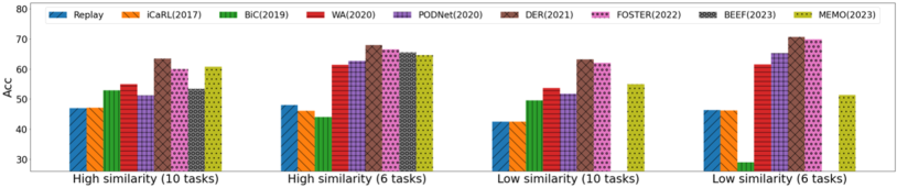
Figure 2: Bar graphs depict the experimental outcomes from the Evaluation phase, with the Y-axis representing the accuracy ($Acc$). Note that FOSTER, BEEF, and MEMO are the current state-of-the-art algorithms. For both scenarios involving 10 and 6 tasks with low similarity, we encountered challenges obtaining the result for BEEF due to a NaN issue in the training loss.

4 Experiments

4.1 Experimental settings

Experimental details   We configured the Hyperparameter Tuning and Evaluation Phases based on the CIFAR-100 [11] and ImageNet-100 [8] datasets. We divided these datasets into disjoint classes, creating CIFAR-50-1, CIFAR-50-2, ImageNet-50-1, and ImageNet-50-2 datasets. We focused on two essential class-incremental learning (CIL) scenarios [14]: 1) 10 tasks: sequentially learning 10 tasks, each composed of 5 classes, 2) 6 tasks: learning 25 classes in the first task and subsequently learning 5 tasks, each consisting of 5 classes.

In the Hyperparameter Tuning phase, we performed experiments on the CIL scenarios generated from the CIFAR-50-1 dataset. We considered 50 random samplings ($R=50$) and 5 trials ($S=5$) for each algorithm to determine the best hyperparameter values. In the Evaluation phase, we considered two scenarios based on similarity between $D^{T}$ and $D^{E}$:

1. High similarity: we generated two CIL scenarios using the CIFAR-50-2 dataset and reported experimental results using the selected best hyperparameter values from the Hyperparameter Tuning phase.

2. Low similarity: two CIL scenarios are generated with the ImageNet-50-2 dataset and conducted CIL experiments following the same process as before.

In the Evaluation phase, we also considered 5 trials ($S=5$) and reported their averaged performance. We trained ResNet-32 and ResNet-18 [10] models for the case of using the CIFAR and ImageNet dataset, respectively. All experiments are conducted based on the CIL benchmark code [29]. The more details are presented in the Supplementary Materials.

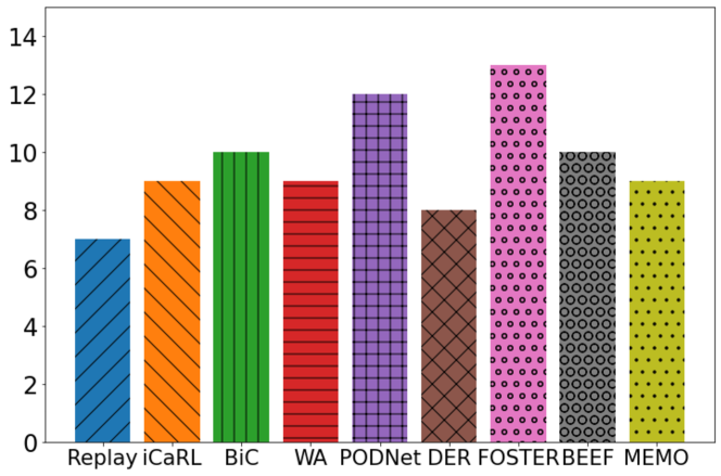
Figure 3: The total number of hyperparameters.

Baselines   As shown in Figure 3, we selected 9 CIL algorithms and conducted experiments using a code implemented in PyCIL [29]. Note that FOSTER [22], BEEF [21] and MEMO [28] are current state-of-the-art algorithms which reported superior performance in CIL compared to other baselines. For all algorithms, we utilized an exemplar memory saving 1000 exemplars. After training each task, we randomly sampled exemplars from the current and the exemplar memory in a class-balanced way. Replay denotes the naive baseline which finetunes a model using both the exemplar memory and the current task’s dataset. During hyperparameter tuning, we adjusted not only additional hyperparameters for each CIL algorithm but also fundamental ones like learning rate, mini-batch size, etc. The total count of hyperparameters for each algorithm, encompassing both additional and basic ones, is displayed in the table. Further details on the selected optimal hyperparameter values and the predefined set of hyperparameter values can be found in the Supplementary Materials.

4.2 Experimental results

Table 1: Experimental results in the Evaluation phase.

Acc / AvgAcc	High similarity ($D^{T}$ = CIFAR-50-1 and $D^{E}$ = CIFAR-50-2)		Low similarity ($D^{T}$ = CIFAR-50-1 and $D^{E}$ = ImageNet-50-2)
	10 tasks	6 tasks	10 tasks	6 tasks
Replay	47.01 / 67.14	48.00 / 59.87	42.51 / 60.71	46.29 / 55.67
iCaRL [18]	47.11 / 66.71	46.09 / 59.14	42.44 / 61.55	46.21 / 57.59
BiC [24]	52.83 / 69.16	44.04 / 53.65	49.52 / 67.09	28.98 / 46.94
WA [27]	54.89 / 69.58	61.37 / 70.56	53.64 / 67.75	61.57 / 69.67
PODNet [9]	51.20 / 69.47	62.62 / 72.62	51.70 / 67.86	65.30 / 73.56
DER [25]	63.51 / 75.04	67.98 / 75.88	63.22 / 72.80	70.68 / 76.56
FOSTER [22]	60.00 / 72.29	66.56 / 73.93	62.09 / 70.24	69.86 / 75.27
BEEF [21]	53.37 / 67.95	65.51 / 72.98	- / -	- / -
MEMO [28]	60.72 / 73.78	64.64 / 73.50	54.91 / 68.06	51.40 / 62.11

As outlined in Section 3, our initial step involves identifying the optimal hyperparameter values for each CIL algorithm using the CIFAR-50-1 dataset. Subsequently, we apply these determined hyperparameter values to each CIL algorithm during the Evaluation phase. The experimental results are visually represented in the bar graphs of Figure 2. For a more comprehensive overview, detailed outcomes for both High and Low similarity scenarios can be found in Table 1 and Figure 4.

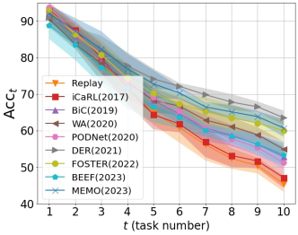
(a) High similarity (10 tasks)

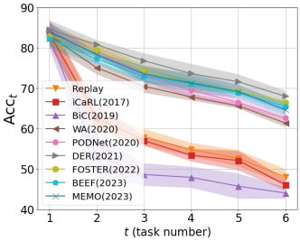
(b) High similarity (6 tasks)

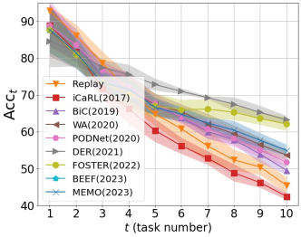
(c) Low similarity (10 tasks)

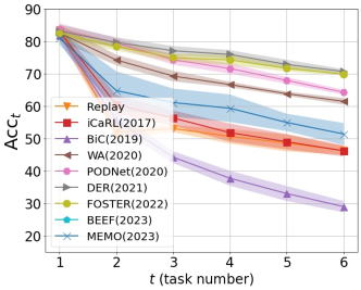
(d) Low similarity (6 tasks)

Figure 4: Experimental results of the Evaluation phase. The shading in each graph represents the standard deviation.

High similarity   From the experimental results presented in both Figure 2 and Table 1, several observations can be derived. Firstly, when employing optimal hyperparameter values, Replay not only achieves performance closely aligned with iCaRL for 10 tasks but also surpasses iCaRL and BiC for 6 tasks. This implies that optimal hyperparameter values for Replay have been overlooked so far, and both iCaRL and BiC do not show the CL capability in our protocol than Replay. Secondly, among non-expansion-based methods, such as Replay, iCarl, BiC, WA, and PODNet, both WA and PODNet demonstrate the most competitive CL capacity. Thirdly, while PODNet doesn’t exhibit impressive results across 10 tasks, it showcases relatively superior CL capacity for 6 tasks. Lastly, despite being considered state-of-the-art algorithms in their respective papers, FOSTER, BEEF, and MEMO reported results that did not surpass DER in our protocol. This implies that their superior performance, as reported in their papers, might stem from significant overfitting to specific datasets and CL scenarios used in experiments. Consequently, they did not demonstrate better CL capacity in our protocol compared to DER, contradicting their reported results. A similar trend is evident for most values of $t$ in both Figure 4(a) and 4(b).

Low similarity   Table 1, Figure 4(c), and Figure 4(d) depict the experimental results for the Low similarity scenario in the Evaluation phase. While we generally observe trends similar to the previous experimental results, a few distinct findings stand out. First, BiC exhibits notably inadequate CL capacity for 6 tasks. Second, DER still demonstrates superior results compared to other current state-of-the-art algorithms, however, MEMO and BEEF still show greater challenges in their CL capacity. Particularly, BEEF displays high sensitivity to hyperparameter values, resulting in a NaN (Not a Number) issue of training loss during the Evaluation phase. Therefore, we could not get the results of BEEF.

These outcomes underscore that many recently reported state-of-the-art CIL algorithms are overestimated in their CL capacity due to an inappropriate evaluation protocol. Moreover, when these algorithms are applied in real-world CIL scenarios, it becomes evident that certain algorithms fail to produce the expected results based on their experimental outcomes. Considering these factors, we contend that our proposed evaluation protocol must be considered to accurately assess the practical CL capacity of each algorithm.

4.3 Experimental analysis

In this section, we conduct further experimental analyses to evaluate the actual benefits of several CIL algorithms in terms of efficiency, focusing on two aspects: the total number of parameters and training time. Both analyses are conducted using models trained by the Evaluation phase involving high task similarity encompassing 10 tasks.

Total number of parameters  Figure 5 illustrates the evolution of the total number of parameters for each algorithm after training task $t$. Four model expansion-based algorithms, namely DER, FOSTER, BEEF, and MEMO, dynamically expand their models after training each task, unlike others. Among them, while DER and BEEF exhibit a linear expansion in model size, FOSTER maintains a twofold increase. These results suggest that despite DER showcasing superior CL capacity within our evaluation protocol, it compromises efficiency due to its larger model size. Additionally, both BEEF and MEMO not only demonstrate ineffectiveness in controlling model size but also result in inferior CL capacities compared to other non-expansion-based algorithms.

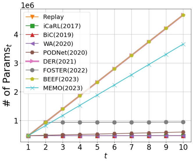
Figure 5: The total number of parameters of each algorithm after training task $t$.

Total training time  As another aspect of our analysis, we compared the total training time, training from task 1 to 10, of each algorithm using optimal hyperparameter values. The results, depicted in Figure 6, encompass both the actual training time for each task and post-training time. Particularly, BiC, FOSTER and BEEF require a significant amount of training time due to the post-training step. Considering that training time directly impacts GPU utilization costs, especially when utilizing commercial GPU services, FOSTER shows relative efficiency in both CL capacity and managing model size but falls short of achieving cost-efficiency in training time. Lastly, BEEF also exhibits the worst inefficiency.

Through our additional analysis, we have found that algorithms with relatively better CL capacity in our proposed evaluation protocol may still lack efficiency in model size and training time. Additionally, we observed that some algorithms, despite their shortcomings, have been overrated due to the current inappropriate and limited evaluation. Based on these findings, we advocate for accurate assessment of each algorithm’s efficiency by evaluating their CL capacity through the proposed protocol and conducting further diverse assessments [4, 17].

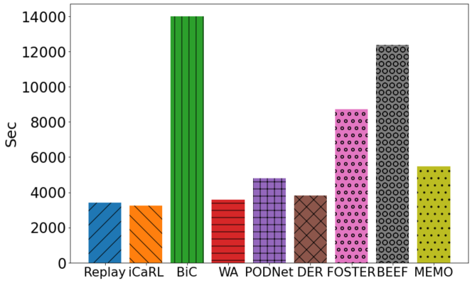
Figure 6: The total training time (in seconds) of each algorithm.

5 Concluding Remarks

We introduced an evaluation protocol aimed at accurately assessing the Continual Learning (CL) capacity of algorithms, adhering to fundamental principles of evaluation in machine learning. This protocol comprises two key phases: Hyperparameter Tuning and Evaluation. In the Hyperparameter Tuning phase, optimal hyperparameter values are determined for each CL algorithm tailored to a specific CL scenario. Subsequently, in the Evaluation phase, these algorithms are trained under identical CL scenarios but with a different dataset, utilizing the optimal hyperparameter values selected from the previous phase. The results obtained in the Evaluation phase serve as a criterion for evaluating the CL capacity of each algorithm. We first applied this proposed evaluation protocol to evaluate class-incremental learning algorithms. The results revealed that the existing evaluation protocol tend to overestimate the CL capacity of these algorithms due to significant overfitting to datasets and CL scenarios. Hence, we argue that to properly assess the CL capacity, it is imperative to conduct evaluations through the proposed protocol.

6 Limitations and Future Work

The proposed evaluation protocol is not limited to a specific CL domain, making it generally applicable to various domains such as online continual learning, class-incremental semantic segmentation, and continual self-supervised learning. From this perspective, we will apply the proposed evaluation protocol to a more diverse set of domains. Moreover, further research on a hyperparameter tuning method is essential to determine hyperparameter values that can successfully apply these CL algorithms to real-world scenarios.

7 Acknowledgement

The work was supported by the National Science Foundation (under NSF Award 1922658) and the Samsung Advanced Institute of Technology (under the project Next Generation Deep Learning: From Pattern Recognition to AI).

Appendix A Additional Experimental Details in Class Incremental Learning Experiments

A.1 Experimental settings

All experiments were conducted based on the code implementation of each algorithm provided by PyCIL [29], applying the proposed two-phase framework. Regarding the learning hyperparameters, it has been observed that achieving a generally high continual incremental learning (CIL) performance is facilitated by differentiating the learning hyperparameters between the first task and the remaining tasks (typically involving more epochs of training in the first task and different learning rates) [14]. As a result, many recent algorithms have adopted such a setup and selected hyperparameter values for training the first task are almost same [9, 25, 22, 21, 28]. To uniformly apply this approach across all algorithms, certain hyperparameter values for the first task learning were fixed, as shown in Table 2. All other hyperparameters and those for the remaining tasks were sampled from the hyperparameter set in Table 3. After the Hyperparameter Tuning phase, the selected optimal hyperparameter values for each algorithm are presented in Table 4.

Table 2: The hyperparmeter values for training the first task.

Hyperparameters	Values
Init epochs	200
Init learning rate	0.1
Init milestones	[60, 120, 170] (but only applied when ’StepLR’ is selected)
Init learning rate decay	0.1
Init weight decay	0.0005

Table 3: The predefined set of hyperparameter values.

	$h^{Set}$
Epoch	160
LR	[30, 70, 120, 160, 200]
Num milestones	[2, 3, 4]
LR decay	[0.05, 0.1, 0.16, 0.2, 0.3]
Batch size	[32, 64, 128, 256, 512]
Weigh decay	[0.0001, 0.0005, 0.001, 0.005]
LR Scheduler	[’StepLR’, ’Cosine’]
T (KD)	[0.5, 1, 1.5, 2, 2.5]
$\lambda$ (KD)	[0.5, 1, 1.5, 2, 3]
Split ratio	[0.05, 0.1, 0.15, 0.2, 0.3]
$\lambda$ (Aux)	[0.5, 1, 1.5, 2, 3]
$\lambda$ (FE)	[0.5, 1, 1.5, 2, 3]
$\beta_{1}$	[0.93, 0.95, 0.97, 0.99]
$\beta_{2}$	[0.93, 0.95, 0.97, 0.99]
Num proxy	[10, 20, 30, 50, 100]
Post FT epochs	[5, 10, 20, 30, 50] / [30, 70, 120, 160, 200] (FOSTER and BEEF)
Post FT LR	[0.001, 0.003, 0.005, 0.007, 0.01]
Energy weight	[0.001, 0.005, 0.01, 0.02, 0.05]
Logit alignment	[1.1, 1.4, 1.7, 2.0, 2.3]
Exemplar batch size	[16, 32, 64, 128, 256]

Table 4: The optimal hyperparameter values found from the Hyperparameter Tuning phase

10 tasks	Epoch	LR	Num milestones	LR decay	Batch size	Weigh decay	LR Scheduler	T (KD)	$\lambda$ (KD)	Split ratio	$\lambda$ (Aux)	$\lambda$ (FE)	$\beta_{1}$	$\beta_{2}$	Num proxy	Post FT epochs	Post FT LR	Energy weight	Logit alignment	Exemplar batch size
FT	160	0.15	-	0.3	32	0.0001	Cosine	-	-	-	-	-	-	-	-	-	-	-	-	-
iCaRL	70	0.05	-	0.3	32	0.001	Cosine	2.5	-	-	1	-	-	-	-	-	-	-	-	-
BiC	200	0.1	-	0.1	32	0.0001	Cosine	0.5	0.5	0.2	-	-	-	-	-	-	-	-	-	-
WA	160	0.05	-	0.1	64	0.001	Cosine	2	3	-	-	-	-	-	-	-	-	-	-	-
PODNet	70	0.1	2	0.1	32	0.0001	StepLR	-	1	-	1	-	-	-	10	30	0.007	-	-	-
DER	200	0.2	-	0.1	256	0.001	Cosine	-	-	-	2	-	-	-	-	-	-	-	-	-
Foster	120	0.1	3	0.5	32	0.001	StepLR	2	1.5	-	-	0.5	0.97	0.93	-	160	-	-	-	-
BEEF	160	0.3	3	0.5	256	0.0001	StepLR	-	-	-	-	-	-	-	-	200	-	0.005	2.3	-
MEMO	120	0.05	4	0.3	32	0.005	StepLR	-	-	-	0.5	-	-	-	-	-	-	-	-	16
6 tasks	Epoch	LR	Num milestones	LR decay	Batch size	Weigh decay	LR Scheduler	T (KD)	$\lambda$ (KD)	Split ratio	$\lambda$ (Aux)	$\lambda$ (FE)	$\beta_{1}$	$\beta_{2}$	Num proxy	Post FT epochs	Post FT LR	Energy weight	Logit alignment	Exemplar batch size
FT	70	0.05	-	0.1	32	0.0001	Cosine	-	-	-	-	-	-	-	-	-	-	-	-	-
iCaRL	120	0.05	-	0.1	32	0.0005	Cosine	1	1	-	-	-	-	-	-	-	-	-	-	-
BiC	200	0.3	3	0.5	128	0.0005	StepLR	1.5	2	0.1	-	-	-	-	-	-	-	-	-	-
WA	160	0.05	-	0.1	64	0.0001	Cosine	2	1.5	-	-	-	-	-	-	-	-	-	-	-
PODNet	30	0.05	-	0.5	64	0.0005	Cosine	-	1	-	3	-	-	-	30	50	0.003	-	-	-
DER	120	0.05	-	0.5	64	0.001	Cosine	-	-	-	1.5	-	-	-	-	-	-	-	-	-
Foster	70	0.05	2	0.1	64	0.0005	StepLR	1.5	1.0	-	-	3.0	0.97	0.93	-	200	-	-	-	-
BEEF	70	0.5	4	0.1	128	0.005	StepLR	-	-	-	-	-	-	-	-	70	-	0.05	2.3	-
MEMO	160	0.05	-	0.1	32	0.001	Cosine	-	-	-	0.5	-	-	-	-	-	-	-	-	256

References

- Aljundi et al. [2018] Rahaf Aljundi, Francesca Babiloni, Mohamed Elhoseiny, Marcus Rohrbach, and Tinne Tuytelaars. Memory aware synapses: Learning what (not) to forget. In Proceedings of the European Conference on Computer Vision (ECCV), pages 139–154, 2018.
- Cha et al. [2021] Sungmin Cha, Hsiang Hsu, Taebaek Hwang, Flavio Calmon, and Taesup Moon. {CPR}: Classifier-projection regularization for continual learning. In International Conference on Learning Representations, 2021.
- Cha et al. [2023a] Sungmin Cha, Sungjun Cho, Dasol Hwang, Sunwon Hong, Moontae Lee, and Taesup Moon. Rebalancing batch normalization for exemplar-based class-incremental learning. In Proceedings of the IEEE/CVF Conference on Computer Vision and Pattern Recognition, pages 20127–20136, 2023a.
- Cha et al. [2023b] Sungmin Cha, Jihwan Kwak, Dongsub Shim, Hyunwoo Kim, Moontae Lee, Honglak Lee, and Taesup Moon. Towards more objective evaluation of class incremental learning: Representation learning perspective, 2023b.
- Chaudhry et al. [2018a] Arslan Chaudhry, Puneet K Dokania, Thalaiyasingam Ajanthan, and Philip HS Torr. Riemannian walk for incremental learning: Understanding forgetting and intransigence. In Proceedings of the European Conference on Computer Vision (ECCV), pages 532–547, 2018a.
- Chaudhry et al. [2018b] Arslan Chaudhry, Marc’Aurelio Ranzato, Marcus Rohrbach, and Mohamed Elhoseiny. Efficient lifelong learning with a-gem. arXiv preprint arXiv:1812.00420, 2018b.
- Delange et al. [2021] Matthias Delange, Rahaf Aljundi, Marc Masana, Sarah Parisot, Xu Jia, Ales Leonardis, Greg Slabaugh, and Tinne Tuytelaars. A continual learning survey: Defying forgetting in classification tasks. IEEE Transactions on Pattern Analysis and Machine Intelligence, 2021.
- Deng et al. [2009] Jia Deng, Wei Dong, Richard Socher, Li-Jia Li, Kai Li, and Li Fei-Fei. Imagenet: A large-scale hierarchical image database. In 2009 IEEE conference on computer vision and pattern recognition, pages 248–255. Ieee, 2009.
- Douillard et al. [2020] Arthur Douillard, Matthieu Cord, Charles Ollion, Thomas Robert, and Eduardo Valle. Podnet: Pooled outputs distillation for small-tasks incremental learning. In Computer Vision–ECCV 2020: 16th European Conference, Glasgow, UK, August 23–28, 2020, Proceedings, Part XX 16, pages 86–102. Springer, 2020.
- He et al. [2016] Kaiming He, Xiangyu Zhang, Shaoqing Ren, and Jian Sun. Deep residual learning for image recognition. In Proceedings of the IEEE conference on computer vision and pattern recognition, pages 770–778, 2016.
- Krizhevsky et al. [2009] Alex Krizhevsky, Geoffrey Hinton, et al. Learning multiple layers of features from tiny images. 2009.
- Li and Hoiem [2017] Zhizhong Li and Derek Hoiem. Learning without forgetting. IEEE transactions on pattern analysis and machine intelligence, 40(12):2935–2947, 2017.
- Liu et al. [2023] Yaoyao Liu, Yingying Li, Bernt Schiele, and Qianru Sun. Online hyperparameter optimization for class-incremental learning. arXiv preprint arXiv:2301.05032, 2023.
- Masana et al. [2020] Marc Masana, Xialei Liu, Bartlomiej Twardowski, Mikel Menta, Andrew D Bagdanov, and Joost van de Weijer. Class-incremental learning: survey and performance evaluation on image classification. arXiv preprint arXiv:2010.15277, 2020.
- Mermillod et al. [2013] Martial Mermillod, Aurélia Bugaiska, and Patrick Bonin. The stability-plasticity dilemma: Investigating the continuum from catastrophic forgetting to age-limited learning effects. Frontiers in psychology, 4:504, 2013.
- Parisi et al. [2019] German I Parisi, Ronald Kemker, Jose L Part, Christopher Kanan, and Stefan Wermter. Continual lifelong learning with neural networks: A review. Neural Networks, 113:54–71, 2019.
- Prabhu et al. [2023] Ameya Prabhu, Hasan Abed Al Kader Hammoud, Puneet K Dokania, Philip HS Torr, Ser-Nam Lim, Bernard Ghanem, and Adel Bibi. Computationally budgeted continual learning: What does matter? In Proceedings of the IEEE/CVF Conference on Computer Vision and Pattern Recognition, pages 3698–3707, 2023.
- Rebuffi et al. [2017] Sylvestre-Alvise Rebuffi, Alexander Kolesnikov, Georg Sperl, and Christoph H Lampert. icarl: Incremental classifier and representation learning. In Proceedings of the IEEE conference on Computer Vision and Pattern Recognition, pages 2001–2010, 2017.
- Schwarz et al. [2018] Jonathan Schwarz, Wojciech Czarnecki, Jelena Luketina, Agnieszka Grabska-Barwinska, Yee Whye Teh, Razvan Pascanu, and Raia Hadsell. Progress & compress: A scalable framework for continual learning. In International conference on machine learning, pages 4528–4537. PMLR, 2018.
- Van de Ven and Tolias [2019] Gido M Van de Ven and Andreas S Tolias. Three scenarios for continual learning. arXiv preprint arXiv:1904.07734, 2019.
- Wang et al. [2022a] Fu-Yun Wang, Da-Wei Zhou, Liu Liu, Han-Jia Ye, Yatao Bian, De-Chuan Zhan, and Peilin Zhao. Beef: Bi-compatible class-incremental learning via energy-based expansion and fusion. In The Eleventh International Conference on Learning Representations, 2022a.
- Wang et al. [2022b] Fu-Yun Wang, Da-Wei Zhou, Han-Jia Ye, and De-Chuan Zhan. Foster: Feature boosting and compression for class-incremental learning. In European conference on computer vision, pages 398–414. Springer, 2022b.
- Wang et al. [2023] Liyuan Wang, Xingxing Zhang, Hang Su, and Jun Zhu. A comprehensive survey of continual learning: Theory, method and application. arXiv preprint arXiv:2302.00487, 2023.
- Wu et al. [2019] Yue Wu, Yinpeng Chen, Lijuan Wang, Yuancheng Ye, Zicheng Liu, Yandong Guo, and Yun Fu. Large scale incremental learning. In Proceedings of the IEEE/CVF Conference on Computer Vision and Pattern Recognition, pages 374–382, 2019.
- Yan et al. [2021] Shipeng Yan, Jiangwei Xie, and Xuming He. Der: Dynamically expandable representation for class incremental learning. In Proceedings of the IEEE/CVF Conference on Computer Vision and Pattern Recognition, pages 3014–3023, 2021.
- Yoon et al. [2017] Jaehong Yoon, Eunho Yang, Jeongtae Lee, and Sung Ju Hwang. Lifelong learning with dynamically expandable networks. arXiv preprint arXiv:1708.01547, 2017.
- Zhao et al. [2020] Bowen Zhao, Xi Xiao, Guojun Gan, Bin Zhang, and Shu-Tao Xia. Maintaining discrimination and fairness in class incremental learning. In Proceedings of the IEEE/CVF conference on computer vision and pattern recognition, pages 13208–13217, 2020.
- Zhou et al. [2022] Da-Wei Zhou, Qi-Wei Wang, Han-Jia Ye, and De-Chuan Zhan. A model or 603 exemplars: Towards memory-efficient class-incremental learning. arXiv preprint arXiv:2205.13218, 2022.
- Zhou et al. [2023] Da-Wei Zhou, Fu-Yun Wang, Han-Jia Ye, and De-Chuan Zhan. Pycil: a python toolbox for class-incremental learning. SCIENCE CHINA Information Sciences, 66(9):197101–, 2023.