Exact theory of the finite-temperature spectral function of Fermi polarons with multiple particle-hole excitations: Diagrammatic theory versus Chevy ansatz
Abstract
By using both diagrammatic theory and Chevy ansatz approach, we derive an exact set of equations, which determines the spectral function of Fermi polarons with multiple particle-hole excitations at nonzero temperature. In the diagrammatic theory, we find out the complete series of Feynman diagrams for the multi-particle vertex functions, when the unregularized contact interaction strength becomes infinitesimal, a typical situation occurring in two- or three- dimensional free space. The latter Chevy ansatz approach is more widely applicable, allowing a nonzero interaction strength. We clarify the equivalence of the two approaches for an infinitesimal interaction strength and show that the variational coefficients in the Chevy ansatz are precisely the on-shell multi-particle vertex functions divided by an excitation energy. Truncated to a particular order of particle-hole excitations, our exact set of equations can be used to numerically calculate the finite-temperature polaron spectral function, once the numerical singularities in the equations are appropriately treated. As a concrete example, we calculate the finite-temperature spectral function of Fermi polarons in one-dimensional lattices, taking into account all the two-particle-hole excitations. We show that the inclusion of two-particle-hole excitations quantitatively improve the predictions on the polaron spectral function. Our results provide a useful way to solve the challenge problem of accurately predicting the finite-temperature spectral function of Fermi polarons in three-dimensional free space. In addition, our clarification of the complete set of Feynman diagrams for the multi-particle polaron vertex functions may inspire the development of more accurate diagrammatic theories of population-imbalanced strongly interacting Fermi gases, beyond the conventional many-body -matrix approximation.
I Introduction
A single impurity interacts with a Fermi sea of ideal, non-interacting fermions, which is the so-called Fermi polaron, is probably the simplest quantum many-body system that one may imagine (Alexandrov2010, ). In the limit of an infinitely heavy impurity, which, to a good approximation, arises in the study of the Fermi edge singularity in x-ray spectra (Mahan1967, ), a highly non-trivial exact solution exists (TextbookMahan2000, ; Roulet1969, ; Nozieres1969a, ; Nozieres1969b, ). As described in detail by Mahan in his classical textbook (TextbookMahan2000, ), the development of such a seemingly simple exact solution is actually not straightforward. In his first investigation of the Fermi edge singularity, Mahan calculated various Feynman diagrams at the high orders of the interaction strength and elucidated that it is inevitable to include the vertex corrections (Mahan1967, ), beyond the many-body -matrix approximation that sums all the ladder diagrams. This insightful observation motivated Nozières and colleagues to consider the parquet diagrams (Roulet1969, ) and eventually fully solve the Fermi edge singularity problem with the parquet equation (Nozieres1969a, ). Interestingly, only after this staggering journey of diagrammatic calculations, which clarify the essence of the Fermi edge singularity, the exact solution starts to emerge (Nozieres1969b, ). Most recently, equipped with a new tool of the functional determinant approach (Levitov1996, ), this exact solution has been used to systematically analyze the quasiparticle properties of heavy Fermi polarons (Knap2012, ; Schmidt2018, ; Wang2022PRL, ; Wang2022PRA, ; Wang2023, ; Wang2023AB, ).
Away from the heavy impurity limit, Fermi polarons turn out to be notoriously difficult to handle, especially when the interparticle interaction between the impurity and the Fermi sea becomes strong. Fortunately, the recent rapid advances in the ultracold atomic research open an entirely new avenue to experimentally explore the Fermi polaron physics (Knap2012, ; Schmidt2018, ; Massignan2014, ; Scazza2022, ). By using various spectroscopic tools, such as the radio-frequency spectroscopy (Schirotzek2009, ; Zhang2012, ; Zan2019, ), Ramsey interferometry (Cetina2016, ), Rabi oscillation (Scazza2017, ; Vivanco2024, ), and Raman spectroscopy (Ness2020, ), quasiparticle properties of Fermi polarons have been quantitatively characterized. These results on the polaron energy, effective mass and quasiparticle residue urgently require the development of an accurate theoretical description of Fermi polarons, particularly on the finite-temperature polaron spectral function, which underlies the various spectroscopic measurements.
A fundamental theoretical framework of Fermi polarons is the so-called Chevy ansatz, which was frequently used by condensed matter community to investigate the Nagaoka ferromagnetism (Nagaoka1966, ) a few decades ago (Shastry1990, ; Basile1990, ; vonderLinden1991, ; Cui2010, ), but re-attracted great attention due to the seminal work by Chevy in 2006 (Chevy2006, ). The Chevy ansatz is generally recognized as a variational approach (Chevy2006, ; Combescot2008, ; Giraud2010, ; Parish2013, ; Liu2019, ; Liu2022, ), which is applicable at zero temperature. It successively takes into account the shake-up process (i.e., the multi-particle-hole excitations) of the Fermi sea due to the interaction with the impurity. Remarkably, already at the first order with only one-particle-hole excitations, the Chevy ansatz works exceptionally well for a strongly interacting Fermi polaron in three-dimensional free space, where the -wave scattering length between the impurity and fermions diverges. It predicts an accurate polaron energy for the ground-state attractive polaron at zero temperature, with a relative error less than , as benchmarked by the ab-initio quantum Monte Carlo simulation (Prokofev2008, ; Pessoa2021, ). Another useful theoretical framework of Fermi polarons is the diagrammatic theory (Combescot2007, ; Hu2018, ; Tajima2018, ; Mulkerin2019, ; Tajima2019, ; Hu2022a, ; Hu2022b, ; Hu2022c, ; Hu2023AB, ; Hu2023, ). Interestingly enough, for Fermi polarons in three-dimensional free space, the Chevy ansatz with one-particle-hole excitations is shown to be fully equivalent to the many-body -matrix theory at zero temperature (Combescot2007, ).
The two theoretical mainstreams, the Chevy ansatz with one-particle-hole excitations and the many-body -matrix theory, have now been widely used to understand the spectroscopic observations of Fermi polarons (Massignan2014, ). They show a great success in predicting the ground-state attractive polaron energy (Massignan2014, ). However, they fail to quantitatively explain the spectroscopic data of the excited states of Fermi polarons at high energy, particularly at nonzero temperature (Tajima2019, ; Hu2022b, ; Hu2022c, ). Other non-perturbative approaches, such as the functional renormalization group (Schmidt2011, ; vonMilczewski2024, ) and quantum Monte Carlo (Goulko2016, ), have also been considered. However, their comparisons with the experimental observations are mostly restricted to the zero-temperature situation.
Theoretically, the failure of the first-order Chevy ansatz and many-body -matrix theory is easy to understand in the heavy polaron limit. In the diagrammatic language, both approaches do not include the important vertex corrections, which should become crucial, as the mass ratio between the impurity and fermions increases (Mahan1967, ; TextbookMahan2000, ). Therefore, to quantitatively understand the current spectroscopic data, we must include the multi-particle-hole excitations of the Fermi sea, both in the Chevy ansatz and in the diagrammatic theory. However, to date, only the effect of two-particle-hole excitations on the attractive polaron energy at zero temperature has been considered (Combescot2008, ; Giraud2010, ; Parish2013, ).
In this work, we formally derive an exact set of infinitely many equations by using both the diagrammatic theory and Chevy ansatz, which can be used to determine the finite-temperature spectral function of Fermi polarons. Our set of equations accounts for arbitrary numbers of particle-hole excitations. Truncated to a particular order , the set of equations encloses and thus provides an approximate theory with the inclusion of -particle-hole excitations of the Fermi sea. At the first order (i.e., ), our theory reduces to the conventional many-body -matrix approximation (Combescot2007, ; Hu2022b, ). However, at higher orders (), the theory gradually adds the non-trivial vertex corrections and should become more accurate.
A brief summary of our work is given in a companion short Letter (ShortPRL2024, ). Here, we would like to highlight a few non-trivial points. First, it is somehow unexpected that we are able to find out the complete Feynman diagrams for the multi-particle vertex functions, which is very rare for quantum many-particle systems. Certainly, this is a peculiar property of Fermi polarons, since the single impurity is only allowed to propagate forward in time (Roulet1969, ). Second, although the first-order Chevy ansatz is shown to be equivalent to the many-body -matrix theory (Combescot2007, ), a general relation between the key variables in the two approaches is not known. Our work clearly reveals that, for an infinitesimal unregularized interaction strength, the variational coefficients in the Chevy ansatz precisely represent the on-shell multi-particle vertex functions in the diagrammatic theory, up to a factor of the excitation energy. This interesting relation demonstrates the powerfulness of the variational approach, as the multi-particle vertex functions are generally impossible to obtain in the diagrammatic theory, even for on-shell values. Finally, despite the exactness of our equations, they suffer from numerical singularities, when some excitation energies become resonant. As a result, the variational coefficients or the on-shell multi-particle vertex functions often vary dramatically. It is interesting to note that, in the heavy impurity limit, the parquet equation used by Nozières and colleagues back to 1960s also suffers from logarithmic singularities (Roulet1969, ), which are tamed through analytic analysis (Nozieres1969a, ). We are optimistic that some clever ideas might be developed in the future analysis of our exact set of equations, with which the singularities could be removed.
The rest of the paper is organized as follows. In the next section (Sec. II), we outline the model Hamiltonian of Fermi polarons. In Sec. III, we construct the diagrammatic theory for an infinitesimal unregularized interaction strength. We explain in detail the structures of diagrammatic representation of multi-particle vertex functions and set up the exact set of equations for the polaron self-energy and hence the polaron spectral function at nonzero temperature. In Sec. IV, we turn to the Chevy ansatz approach with a general nonzero interaction strength. We derivate the equations satisfied by the variational coefficients, with the inclusion of arbitrary numbers of particle-hole excitations. We also consider the specific case of a vanishingly small interaction strength and simplify the equations for the variational coefficients. In Sec. V, we show that the same exact set of equations for the multi-particle vertex functions can be recovered, if we identify the variational coefficients as the on-shell multi-particle vertex functions divided by the excitation energy. In Sec. VI, we discuss the singularities in the derived exact set of equations and propose that, for Fermi polarons in lattices, the singularities might be removed by introducing a finite broadening factor and then extrapolating it to zero. We consider Fermi polarons in one-dimensional lattices as a concrete example, and numerically determine the finite-temperature polaron spectral function, with the inclusion of two-particle-hole excitations. Finally, Sec. VII is devoted to the conclusions and outlooks.
II Model Hamiltonian
We consider a population imbalanced spin-1/2 Fermi gas in free space or within lattices. In the extremely imbalanced limit, i.e., one spin-down fermion immersed in a Fermi sea of spin-up fermions, we treat the spin-down fermion as the impurity (Massignan2014, ; Schirotzek2009, ). The system is then well described by the model Hamiltonian, , where
| (1) | |||||
| (2) |
For clarity, we have suppressed the system volume. Here, and are the creation field operators for spin-up fermions and the impurity, with single-particle dispersion relations and , respectively. In free space, and and we allow different masses and for spin-up fermions and the impurity, respectively. In lattices, for example, in one-dimensional lattices, we would instead have and , where the mass difference is represented by the different hopping strength of spin-up fermions () and of the impurity () on the lattice. In the interaction Hamiltonian , is the interaction strength of the zero-range contact interaction potential (in free space) or of the on-site interaction (in lattices). The Dirac delta function ensures the momentum conservation during the interparticle collisions.
In two- or three-dimensional free space, it is well-known that the -wave contact interaction is not physical at high energy scale (i.e., above a momentum cut-off ) and we need to regularize the associated ultraviolet divergence (Hu2006, ; He2015, ). For example, in three dimensions we should replace the running interaction strength with a given -wave scattering length ,
| (3) |
where is the reduced mass. It is easy to see, the interaction strength becomes infinitesimal, when we tune the cut-off to be infinitely large. This is exactly the case that we will consider in the next section of the diagrammatic theory. In contrast, in lattices, the interaction strength takes a finite value, either attractive or positive.
III The diagrammatic theory
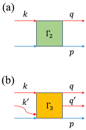
In the diagrammatic theory, the fundamental quantities that we need to look after are the vertex function (see Fig. 1(a)) and the multi-particle (i.e., particles with ) vertex functions (TextbookMahan2000, ; Giraud2010, ; TextbookAGD1975, ),
| (4) |
which describes the scatterings among spin-up fermions in the Fermi sea and the impurity. These in-medium scatterings occur in the presence of the Fermi sea, so more fermions other than the spin-up fermions may participate at the intermediate stages. The momentum , where , is the four-momentum of the -th incoming fermion line, involving both the spatial momentum and the fermionic Matsubara frequency with an integer at the temperature (TextbookMahan2000, ; TextbookAGD1975, ). In a similar way, we use the momentum to denote the four-momentum of the -th out-going fermion line. In addition, we use to label the four-momentum of the out-going impurity line. For small values of , i.e., or , for convenience we also use , , , and so on. The similar notations hold for the out-going momentum ; see, for example, Fig. 1(b) for the three-particle vertex function .
For with , the multi-particle vertex functions with more than one incoming fermion line, we may have a freedom to pick up the line that interacts first with the impurity. As a convention, we will always select the last incoming fermion line with the momentum (Giraud2010, ). This convention is useful for the contact interaction, where the many-body -matrix depends only on the total momentum. As we shall see, the information of is then lost and the -particle vertex function becomes independent on . We note also that, following the Fermi statistics, the remaining incoming fermion lines should be indistinguishable. As a result, the multi-particle vertex function would acquire a minus sign, if we exchange any two momenta among , , . The same antisymmetrization requirement holds, upon exchanging any two out-going momenta among , , .
III.1 Vertex function
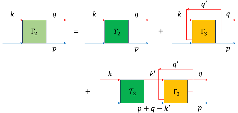
Let us first consider the diagrammatic representation of the vertex function (Giraud2010, ). As shown in Fig. 2, we may identify three contributions. The first contribution is simply the familiar may-body -matrix that takes into account the successive scatterings between a spin-up fermion and the impurity (i.e., ladder diagrams) (Combescot2007, ; Hu2022b, ), without the involvement of any other fermions in the Fermi sea. It depends on the argument only, since we consider a zero-range contact interaction for the impurity-fermion scattering.
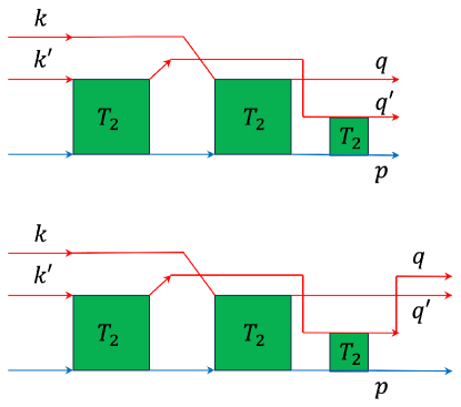
The other two contributions necessarily involve the three-particle vertex function, as we can see from the second and third diagrams on the right-hand-side of Fig. 2. For the second diagram, we wind one out-going fermion line (with the momentum ) back and connect it to the incoming fermion line with the momentum , so . It does not matter to wind the out-going or line, since these two lines are chosen to be antisymmetric and therefore we would obtain the exactly same contribution. But, why we connect the out-going line with to the incoming line with the momentum ? Logically, we could also connect it to the upper incoming line with the momentum . This way of connection is actually realized in the next third diagram, as shown at the bottom of Fig. 2. There, the first diagram () and the second diagram that we have already been considered naturally connect (see, for example, the diagram in Fig. 3, and imagine to connect the -line with the -line).
Now, we would like to claim that we exhaust all the possibilities for constructing the vertex function . One may wonder that for the last diagram in Fig. 2, we can obtain a new contribution if we exchange the two blocks of and . It is actually not true. This is because the three-particle vertex function itself involves a lot of diagrams. If we attach the many-body -matrix to the right-hand-side of the three-particle vertex function , what happens is that the block will be naturally absorbed into the block, giving a contribution that we have already taken into account. Moreover, there are no new contributions related to higher-order vertex functions such as , and so on, as their appearance is implicitly included in the three-particle vertex function and we need to avoid the double counting of diagrams. To see these, let us carefully examine the diagrammatic representation of the three-particle vertex function , which is given in Fig. 3.
III.2 Three-particle vertex function
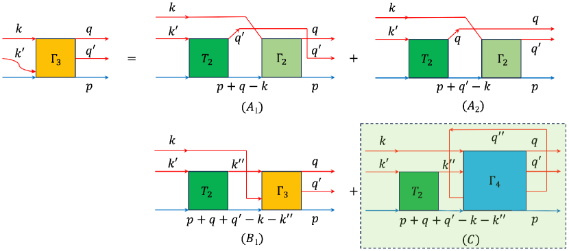
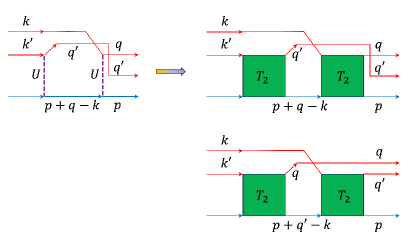
There are four diagrams contributed to , which might be categorized into three different types. To understand the first two contributions in Fig. 3() and Fig. 3(), which are referred to as the -type diagrams, let us recall one of the lowest order diagrams of , measured in terms of the impurity-fermion interaction strength , as given in the left panel of Fig. 4. As we emphasized earlier, since we use the zero-range contact interaction, the interaction strength effectively scales to zero when we increase the cut-off momentum. To have a nonzero contribution, we then need to replace the bare interaction line (i.e., the dashed line) in the left panel of Fig. 4 everywhere by the many-body -matrix . This replacement leads to the building blocks of the three-particle vertex function , as illustrated in the right panel of Fig. 4. Of course, we may continue to consider higher order scattering processes, with the two simplest examples illustrated in Fig. 5. It is not difficult to see that, some of the higher order scattering processes could be easily taken into account, by simply replacing in the two building blocks (i.e., the right panel of Fig. 4) the second with the vertex function . This replacement leads to the two -type diagrams, and , in Fig. 3.
This replacement, however, does not exhaust all the possibilities for constructing . Indeed, it is readily seen that in the building blocks, we may replace the second by the three-particle vertex function itself, and then connect the out-going fermion line of the first to the first incoming fermion line of . This gives rise to the -type diagram, , in Fig. 3.
Finally, similar to what we have observed in constructing the vertex function , we would have contributions to that involves a higher order vertex function . This is given in the last -type diagram in Fig. 3.
In all the diagrammatic contributions to , we see clearly the involvement of the many-body -matrix . It simply follows our definition of the multi-particle vertex functions, as we impose the constraint that the last incoming fermion line must interact first with the incoming impurity line. We will see that the higher order vertex functions such as share the same feature.
III.3 Higher order vertex functions
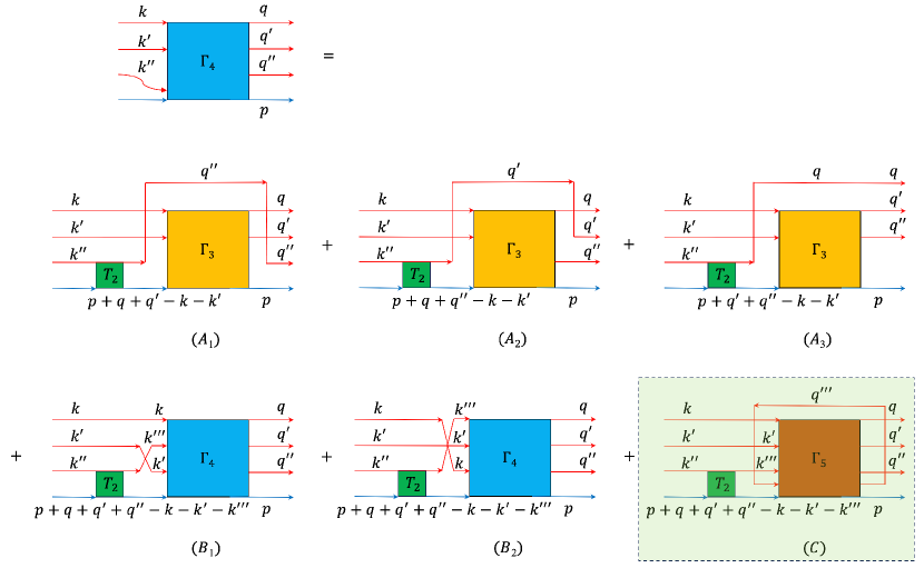
Actually, for all the higher order vertex functions, we have a stronger conclusion that they all can be categorized into the similar three different types. In Fig. 6, we show the diagrammatic representation of the four-particle vertex function as an example and explain the general rules to draw the three kinds of diagrams for the -particle vertex function .
First, the -type diagrams consist of a many-body -matrix and a lower order -particle vertex function . The out-going fermion line of is one of the out-going fermion line of the whole diagram; see, for example, the , and diagrams in Fig. 6. Thus, we have choices to place the out-going fermion line of , which leads to type- diagrams, listed as , , .
Second, the -type diagrams involve a many-body -matrix and the same order -particle vertex function . The out-going fermion line of needs to connect with one of the incoming fermion lines of , apart from the last incoming fermion line. Otherwise, we will obtain itself. Therefore, in total there are type- diagrams, listed as , , .
The final -type diagram is constructed by connecting a many-body -matrix to a higher order -particle vertex function . It is not difficult to see that we only have one possibility: we need to connect the last out-going fermion line of to the last incoming fermion line of , owing to the antisymmetrization of .
III.4 Explicit expressions of various vertex functions
The determination of the complete set of the diagrams for each multi-particle vertex function allows us to directly write down its expression, in terms of the Green functions of the spin-up fermions and of the impurity Green function , and of the multi-particle vertex functions themselves. However, specific attention should be paid to the overall sign of each diagram, as we shall explain in detail.
For example, let us write down the expression for the vertex function , following its diagrammatic representation in Fig. 2,
| (5) |
Here, by default the summation (or ) is understood as (or ) for the four-momentum (or ) (TextbookMahan2000, ; TextbookAGD1975, ). Each term on the right-hand-side of Eq. (5) corresponds to a diagram in Fig. 2. We note that, in the expression of , we have suppressed the argument of , as is independent on it.
The second term comes with a positive sign, although there is a Fermi loop in the corresponding diagram (i.e., the second diagram on the right-hand-side of Fig. 2), which contributes a minus sign (TextbookMahan2000, ; TextbookAGD1975, ). This minus sign is actually cancelled by the minus sign we wish to assign to the three-particle vertex function . Indeed, here we encounter a potential ambiguity for the sign of . Let us recall the two building blocks of , as illustrated in the right part of Fig. 4. These two diagrams look very similar and differ only by exchanging the two out-going fermion lines. Of course, this exchange means a sign difference. But, which diagram has the positive sign? We naturally assume that the upper building block of has the positive sign and write down in an abbreviated form , where the tilde on stands for the contribution from the upper building block to . Now, let us insert this upper building block of into Fig. 2. Following the standard rules, we may write down its contribution to , i.e., , again in an abbreviated form. Here, the first minus sign comes from the Fermi loop and the second minus sign is because the diagram appears to be an order higher in the interaction line (or in ), when we replace with the upper building block of . In brief, the three-particle vertex function acquires a minus sign, if we fix the sign convention for its two building blocks given in the right panel of Fig. 4. Following such a convention, we can easily understand the minus sign appearing in the third term of Eq. (5), as the corresponding diagram is an order higher in .
For the expression of the three-particle vertex function , according to Fig. 3 we may formally write down,
| (6) | |||||
where the four terms on the right-hand-side of the equations comes from the diagrams , , and , respectively. The signs of the first two terms have already been discussed, since the diagrams and have the exactly same topology as the two building blocks of . More generally, we will always fix the sign of the -diagram for any multi-particle vertex functions to be positive. The sign of the -diagram () will then be . Following this convention, it is not difficult to see that we need to assign a minus sign to in relative to . As a result, all the -type diagrams come with a negative sign.
It is a bit tricky to determine sign of the diagram in Fig. 3. A convenient way is to compare the diagram with the diagram. These two diagrams have one feature in common: if we connect the out-going -line with the incoming line, no Fermi loop is created. Thus, naïvely, we anticipate that topologically the diagram will have the same sign as the diagram. However, as involves instead of , an additional sign appears. This additional sign will cancel the minus sign of the diagram. In the end, we find a positive sign for the diagram. In the general case for any multi-particle vertex functions , we might see that the sign of the -type diagram () is always positive, in order to satisfy the requirement that there should be a sign difference if we exchange any two momenta in .
It is easy to check that the right-hand-side of Eq. (6) does not contain the momentum , justifying our previous statement that does not depend on the last incoming momentum .
We are now ready to write down the general expression for the multi-particle vertex function (),
| (7) |
where by default the index runs from to , and
| (8) | |||||
| (9) | |||||
| (10) |
In , the argument is absent in . As explained in detail in Appendix A, a sign factor arises due to the antisymmetrization among . In , the argument of is located at the position . always has a positive sign. We acquire a sign factor of if we move the argument all the way to the right-hand-side of . The sign factor then makes antisymmetric, upon the exchange of any two momenta among .
Eq. (5) for and Eq. (7) for form a complete set of equations to determine all the vertex functions. This set of equations encloses at a particular order , if we discard the -term in . In particular, if we neglect the last shaded diagrams in Fig. 3 or in Fig. 6, we have the enclosed set of equations to calculate the vertex functions, with the inclusion of two-particle-hole excitations or three-particle-hole excitations.
III.5 Dyson equation for the polaron self-energy
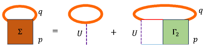
As we are interested in obtaining the polaron spectral function, another fundamental quantity is the polaron self-energy , whose diagrammatic representation is given in Fig. 7, according to the well-known Dyson equation (TextbookAGD1975, ). As the interaction strength is infinitesimal, the first Hartree diagram with a single dashed line does not contribute. For the second diagram, we may write down,
| (11) |
where we have introduce a new variable
| (12) |
Therefore, we may directly calculate the self-energy , once we obtain the vertex function . In turn, we determine the impurity Green function (),
| (13) |
and obtain the polaron spectral function (TextbookMahan2000, ; TextbookAGD1975, ).
III.6 On-shell vertex functions
We now have an exact set of expressions, each of which involves the summation over four-momenta. Here, we would like to point out that, in the single-impurity or polaron limit, the summation over the fermionic Matsubara frequency can be explicitly carried out (Combescot2007, ; Hu2022b, ). As we shall see, we have the summation over the two kinds of four-momentum. The one denoted by the variables (or ) is particle-like and is the momentum of a fermion line propagating forward. For example, we have the summation , where the function contains the particle-like momentum and other variables in , and does not have any singularity at positive energy. Another is hole-like and is the momentum of a Fermi loop moving backward. It will be denoted by the variables (or ), so we have the summation such as , where the function is analytic on the left half-plane with negative energy.
As discussed in detail in Appendix B, we find two simple rules related to the summation over the fermionic Matsubara frequency part of and ,
| (14) | |||||
| (15) |
where is the Fermi-Dirac distribution function, and and are the dispersion relations of fermions, measured from the chemical potential . In other words, the action of the summation over the fermionic Matsubara frequency merely turns the varying Matsubara frequency into an on-shell value, either or , with a weighting factor of or , which is related to the thermal occupation of quasiparticle states, for either particles or holes.
By applying these two rules for the summation over the fermionic Matsubara frequency (i.e., for the particle-like momentum and hole-like momentum, respectively), it is straightforward to obtain from Eq. (5) that,
| (16) |
where we have now used the notations } and . From this expression, it becomes clear that we only need to take care of the vertex functions with on-shell four-momenta. For example, in the vertex function , we could take and , as the information of off-shell values is completely not needed. Hereafter, we will always assume the on-shell values for any four-momentum. Of course, the four-momentum for the impurity is special. Here, the spatial momentum and the energy are the given input parameters, for the calculation of the polaron spectral function. For the (on-shell) three-particle vertex function, we then similarly obtain its expression,
| (17) | |||||
Finally, for the self-energy we obtain
| (18) |
where
| (19) |
By using Eq. (16) to replace in , we find an alternative expression for ,
| (20) |
which differs from only by a term , i.e., the second term in Eq. (16). To understand the difference, we note that, to derive Eq. (20), we have used the identities,
| (21) |
and
| (22) |
Both identities are related to infinitesimal running interaction strength . In the former identify, at large momentum and therefore diverges. This divergence is precisely compensated by the infinitesimal , according to our regularization recipe Eq. (3). In contrast, in the latter identity, should decay fast enough at large momentum and the integral becomes finite. The smallness of the running interaction strength then makes the term to vanish.
As a brief summary, we have obtained an exact set of equations to determine the polaron spectral function. It consists of Eq. (18) and Eq. (20) for the self-energy, Eq. (16) and Eq. (17) for the vertex function and the three-particle vertex function, as well as Eq. (7), which, after we integrate out the fermionic Matsubara frequency, gives the on-shell multi-particle vertex functions . and so on.
To close this subsection, it is worth noting that, the use of an infinitesimal contact interaction strength plays an important role to determine the complete sets of diagrams for the multi-particle vertex functions. It enables us to replace the bare, running interaction strength everywhere by the many-body -matrix , as a Feynman diagram with a finite number of the dashed interaction line must vanish. Without this useful property, we will end up with infinitely many messy Feynman diagrams, which we may hardly sum up, even at the first order of taking only one-particle-hole excitations.
III.7 Two-particle-hole excitations
In Eq. (20) for , if we only keep the first term , we are able to calculate the self-energy Eq. (18) with one-particle-hole excitations only (Combescot2007, ; Hu2022b, ). To include two or more particle-hole excitations, we need to keep the second term related to in Eq. (20) and it is necessarily to determine the three-particle vertex function in Eq. (17), which in turn may require the knowledge of . Actually, the exact set of equations that we have just derived has a very nice structure in hierarchy. For example, as we discussed earlier, in Eq. (7) for the multi-particle vertex function , if we discard the last -term, then the set of equations encloses, up to the approximation of including -particle-hole excitations. Here, we would like to present the detailed equations up to the level of including two-particle-hole excitations, which gives the first non-trivial vertex correction, beyond the many-body -matrix theory of Fermi polarons.
For this purpose, for a given four-momentum , it is useful to define the new variables,
| (23) | |||||
| (24) | |||||
| (25) |
where is basically the excitation energy of one-particle-hole excitations, if we take . The equation for the three-particle vertex function Eq. (17) then turns into,
| (26) |
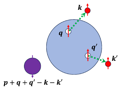
where is the excitation energy of two-particle-hole excitations, if we again take ; see, for example, Fig. 8. The equation for , Eq. (20), takes the form,
| (27) |
In turn, the vertex function is now given by,
| (28) |
Eq. (26), Eq. (27), Eq. (28), together with the definition of , form a closed set of equations, which can be solved to determine the self-energy . To make the equations complete, we also list the explicit expression of the many-body -matrix (Hu2022b, ),
| (29) |
where the running interaction strength is to be replaced by the -wave scattering length , for example, by using Eq. (3) in three dimensions.
IV Chevy ansatz
Let us now turn to consider the Chevy ansatz approach (Chevy2006, ; Combescot2008, ; Liu2022, ). Chevy ansatz has been widely used as a variational approach at zero temperature. Its finite-temperature extension has also recently been considered, with the inclusion of one-particle-hole excitations (Liu2019, ). Here, we aim to generalize Chevy ansatz to finite temperature, including arbitrary numbers of particle-hole excitations. We would like to comment from the beginning that, at nonzero temperature, it probably does not make sense to emphasize the variational aspect of Chevy ansatz, since the polaron state is no longer a single quantum many-body state. Therefore, even for the attractive polaron, its energy at a given finite temperature may increase with the inclusion of more particle-hole excitations. Actually, as we shall see, the most important feature of Chevy ansatz is the closure of the Hilbert space for available quantum states, if we truncate the ansatz to a particular level of -particle-hole excitations. This may also explain why we can find out the complete set of diagrams for the multi-particle vertex functions, as we discussed in the last section.
IV.1 Chevy ansatz at finite temperature
Following the seminal works by Chevy (Chevy2006, ) and Combescot and Giraud (Combescot2008, ; Giraud2010, ), we take the following Chevy ansatz for Fermi polarons (with momentum ),
| (30) | |||||
| (31) |
where describes a thermal Fermi sea at finite temperature, in which the occupation of a single-particle state with momentum is given by the Fermi-Dirac distribution function . At zero temperature, we can find the sharp Fermi surface located at the Fermi wavevector and clearly distinguish a particle excitation with from a hole excitation with . At nonzero temperature, the Fermi surface becomes blurred. Nevertheless, we will relax our definition of particle or hole excitations. We may still use to denote a “particle”-like state out of the Fermi sea and to denote a “hole”-like state within the Fermi sea. It is also convenient to use the abbreviations, , , and . In the case of potential confusion, we will take the full labelling.
It is important to note that, the definition of the coefficients in our ansatz Eq. (31) is slightly different from what used in the earlier works (Chevy2006, ; Combescot2008, ; Giraud2010, ; Liu2022, ). Here, we re-arrange the order of the annihilation field operators in the ansatz. For example, for the two-particle-hole excitation term, we use , instead of . This re-arrangement is crucial to establish the relationship with the diagrammatic theory in the last section. It will also remove some unnecessary signs for the general expressions of the coupled equations for the coefficients. We note also that, in the Chevy ansatz the coefficients should be antisymmetric with respect to the exchange of and or the exchange of and . As a consequence, there are a lot of identical terms in Chevy ansatz, i.e., terms, since the permutations either in or in generates a factorial . This redundancy can be simply removed by the factor .
Our task now is to formally solve the stationary Schrödinger equation, , and derive the set of equations satisfied by the coefficients . To proceed, it is useful to introduce some new variables. We will use
| (32) |
to describe the shake-up Fermi sea with a -particle-hole excitation out of . It has a momentum and an excitation energy . Thus, the -th component of the Chevy ansatz, , is given by,
| (33) |
Let us check the results of .
The action of the non-interacting, kinetic part of the Hamiltonian, (or specifically ), is straightforward to calculate. The creation field operator creates an impurity with single-particle energy , which is to be picked up by the term in . In a similar way, the total single-particle energy of is , where is the energy of the unperturbed Fermi sea at finite temperature. This total single-particle energy will be picked up by the term in . Putting together, we obtain,
| (34) |
On the other hand, the action of the interacting Hamiltonian on the wave-function, , is not so obvious to determine. As involves only a single impurity with momentum , the action of the operators simply changes the momentum of the impurity to . In contrast, as the perturbed Fermi sea state involves infinitely many spin-up fermions, the action of on should be analyzed carefully. In addition to an overall Hartree shift , where is the density of spin-up fermions, generally we find three different situations, referred to as the -, -, and -cases, if we analyze the sector of the -particle-hole excitations for .
In the -case, we consider the action of on , which creates a new particle-hole excitation (where is the particle momentum and is the hole momentum), on top of the existing -particle-hole excitation. The resulting state is , where the prime indicate a new set of particle or hole momenta.
In the -case, we take the action of on , which does not change the number of particle-hole excitations (i.e., we will end up with ). Therefore, it is necessarily to destroy an existing particle state or hole state in . We also need to trace the momentum of this particle state or hole state, over the existing momenta or .
In the -case, we apply the operators on . In order to bring the state back to as we wish to focus on the sector of -particle-hole excitations, we need to destroy both a particle state (with the momentum ) and a hole state (with the momentum ) in .
By enumerating all the possibilities, after a lengthy algebra, we obtain (),
| (35) |
where
| (36) | |||||
| (37) | |||||
| (38) |
All the three coefficients , , are manifestly antisymmetric with respect to the exchange of any two momenta in or . The two Fermi distribution functions and represent the availability of the particle state (with the momentum ) and of the hole state (with the momentum ), respectively. In the expression of , a minus sign arises, simply because, to destroy a hole state we need to rewrite in the interaction Hamiltonian.
We are now ready to translate the stationary Schrödinger equation, , into a set of equations for the coefficients . For this purpose, let use define the excitation energy,
| (39) |
In the absence of the interaction , is precisely the energy cost for the creation of a -particle-hole excitation out of the Fermi sea, if we take . In terms of , we find that the coefficients satisfy a series of coupled equations,
| (40) | |||||
These equations connect the -th coefficients to the lower order -th coefficients (see, i.e., the first term in the right-hand-side of the equation) and the higher order -th coefficients (see the last term). The coupled equations will enclose, if we neglect the last term, yielding the results valid for the inclusion of -particle-hole excitations.
IV.2 Chevy ansatz with two-particle-hole excitations
To illustrate the usefulness of the exact set of equations Eq. (40), let us truncate to the order of , as an example,
| (41) | |||||
| (42) | |||||
| (43) |
Here we define as the energy of the Fermi polaron with the exclusion of the mean-field Hartree shift . The explicit expressions of and are given by, and , respectively.
At zero temperature, where the Fermi distribution functions and respectively restrict the momentum and , the above three equations have already been used to determine the attractive Fermi polaron energy in free space, from one dimension to three dimensions (Combescot2008, ; Parish2013, ). At nonzero temperature, we may discretize the momentum in the equations to obtain the discrete polaron energy levels. However, it will be more interesting to work with continuous momentum. In this case, we may replace the energy by a frequency . We may take , if we do not care about the normalization of the Chevy ansatz. As we shall see, the term can then be understood as the polaron self-energy at the given frequency .
To formally solve the coupled equations (at a given frequency and a given momentum ), it is useful to define several variables,
| (44) | |||||
| (45) | |||||
| (46) | |||||
| (47) | |||||
| (48) |
For convenience, we often use the short-hand notations, and . One may wonder that the short-hand notation has already used for the three-particle vertex function in the diagrammatic theory. We will soon see that there is no contradiction, as they are essentially the same quantity. According to these definitions, we must satisfy the consistency conditions,
| (49) |
and
| (50) |
The first equation Eq (41) then turns into ( and ),
| (51) |
which determines the pole of the polaron Green function. The second equation Eq. (42) becomes,
| (52) |
Let us multiply on both sides and integrate over , or multiply on both sides and integrate over . These operations lead to two coupled equations,
| (53) | |||||
| (54) |
For the third equation Eq. (43), we similarly find,
| (55) |
The integration over or then leads to the coupled equations,
| (56) | |||||
| (57) |
Eq. (53), Eq. (54), Eq. (56), and Eq. (57) form a closed set of coupled equations, together with the expressions of and , Eq. (50) and Eq. (52). They might be numerically solved in a self-consistent way, for any values of the interaction strength . However, to make the connection with the diagrammatic theory, let us first check the case .
IV.3 Chevy ansatz at
As we mentioned earlier, in two-dimensional or three-dimensional free space, the contact interaction potential needs regularization, since the integration over the high momentum diverges. Thus, we effectively have a vanishingly small interaction strength . In this case, the coupled equations of the Chevy ansatz solution Eq. (40) could be simplified.
To find the rules of simplification, let us check the case of two-particle-hole excitations. In the expressions for and , see Eq. (54) and Eq. (57), since the integration over (or ) is finite, we have and , which are both infinitesimally small. Therefore, and . In general, in Eq. (40), the third term on the right-hand-side of the equation vanishes identically. Moreover, in the expression for , Eq. (56), it is easy to see that,
| (58) |
since the integration over converges due to the well-behaved coefficients and at large momentum . Also, we would have,
| (59) |
due to our regularization relation Eq. (3) (i.e., the smallness of exactly cancels the divergence of the integral over ). More generally, therefore, only a few sub-terms in the first term of Eq. (40) contribute. In fact, there are sub-terms in total. However, only sub-terms contribute. Following these observations, for , let us define the variables,
| (60) |
It is then straightforward to derive the equation for :
| (61) | |||||
In the first term on the right-hand-side of the equation, only the sub-terms with a fixed set of indices survive. When we exchange any two indices in the set , the sign ensures that the first term is antisymmetrized, see, for example, Appendix A. In each sub-term of the second term , we will find a sign factor , if we move the momentum to the right-hand-side of . This sign factor has the similar effect for antisymmetrization. When we exchange any two indices in the set , the second term that consists of sub-terms is antisymmetrized. Moreover, there is only one item in the last term, which involves a higher order . We will make the coupled equations enclosed, if we drop this last term and truncate to the level of -th particle-hole excitations.
As a concrete example, up to the level of three-particle-hole excitations, we obtain the coupled equations (by default, we take and ),
| (62) | |||||
| (63) | |||||
| (64) |
Here, in the first equation Eq. (62) we would like to keep the notation of , instead of using . In the last equation Eq. (64), we have dropped the last term that is related to the higher order (or more precisely, ).
V Diagrammatic theory versus Chevy ansatz
It is readily seen that Eq. (7) from the diagrammatic theory and Eq. (61) from the Chevy ansatz approach have the same structure. Moreover, when we take the on-shell values for and , by using the explicit expression of the many-body -matrix , Eq. (29), we immediately identify (),
| (65) |
As both Eq. (7) and Eq. (61) are derived in an exact manner under the same conditions, we conclude that they must be the same equation. By comparing the corresponding terms in the two equations, therefore, we should have the relations,
| (66) | |||||
| (67) |
where in the multi-particle vertex function and , we need to take the on-shell values for all the four-momenta and . Now, we would like to claim that the second relation Eq. (67) is more fundamental than the first relation Eq. (66), in the sense that we can derive Eq. (66) by using Eq. (67). To see this, let us rewrite Eq. (67) into the form,
| (68) |
where we have used the fact that,
| (69) |
As we emphasized earlier, has a unique feature that it is independent on the four-momentum . The -dependence of therefore only comes from or . This feature has an interesting consequence, if we calculate by using its definition,
| (70) |
The integral over in the above equation diverges and when it multiplies with the vanishingly small , we obtain , due to the regularization relation Eq. (3). Thus, we immediately recover Eq. (66), as promised.
To directly show the usefulness of the two relations, Eq. (68) and Eq. (66), let us apply them to the four-particle vertex function with . From Fig. 6, we may write down the following expression for the diagrams:
| (71) |
where the expressions of () are,
| (72) | |||||
| (73) | |||||
| (74) |
and the expressions of , and , after the Matsubara frequency summation, are given by,
| (75) | |||||
| (76) | |||||
| (77) |
It is straightforward to apply Eq. (68) to and to verify , , and , which are the first three terms in the square bracket of the right-hand-side of Eq. (64). Moreover, by using the following relation with on-shell momenta,
| (78) |
and by applying Eq. (66) in to replace , we find that the last two terms in the square bracket of Eq. (64) correspond to and , respectively. It is also not difficult to verify that, the dropped higher order term in Eq. (64) is given by . In this way, we directly reproduce the Chevy ansatz result of Eq. (64), by applying the diagrammatic theory.
VI Fermi polarons in one-dimensional lattices
We now turn to consider the numerical calculations of the polaron spectral function, beyond the commonly-used approximation of including just one-particle-hole excitations. However, at finite temperature there is a serious numerical problem related to the zeros of the excitation energy , which create a lot of singularities (i.e., poles) in the coefficients and , as can be clearly seen from the relation Eq. (68). These singularities make it impossible to directly calculate the various integrals appearing in the exact set of the coupled equations, Eq. (7) or Eq. (61). This numerical problem exists even at zero temperature, if we want to study the repulsive polaron branch at positive energy.
To overcome the numerical difficulty, we may introduce a finite broadening factor to the frequency (i.e., ). Here, for simplicity, we focus on the case of one-dimensional lattices, where the value of momentum is restricted to the first Brillouin zone. We will consider the inclusion of two-particle-hole excitations. A slight inconvenience is that the on-site interaction strength is nonzero. Therefore, we must solve the coupled equations Eq. (53), Eq. (54), Eq. (56) and Eq. (57), with momentum and at a finite broadening factor . Eventually, we extrapolate to zero and obtain the -independent polaron self-energy in Eq. (51) and hence the polaron spectral function.
In future studies, this numerical trick might be extended to the three-dimensional free space, with some improvements. With more elaborate numerical efforts, then we may calculate the more interesting finite-temperature spectral function of a unitary Fermi polaron.
VI.1 Numerical procedure
In one-dimensional lattices, we take and . Typically, we set the energy scale . The hopping strength of the impurity is determined by the mass of the impurity, since . At finite temperature, the chemical potential is to be fixed by the filling factor . We perform numerical calculations for a given momentum and a given energy , so and . Our numerical procedure consists of the following three steps.
-
•
Step 1. For a given , which initially is zero, we iteratively solve the coupled equations Eq. (53) and Eq. (54). To check convergence, we compare with a previously saved (which is zero from the beginning as well). If the difference is smaller than a certain criterion (i.e., the average difference in relative is smaller than ), we jump to Step 3; otherwise, continue with Step 2.
-
•
Step 2. For and generated from Step 1, we iteratively solve the coupled equations Eq. (56) and Eq. (57) for and . As this is a very time-consuming procedure, we do not require the full convergence and the iteration lasts for a few times (we typically choose 8 times). Also, since and , we only need to calculate the case with and . In each interaction, will be updated. We use the two ways to calculate , by using and , and monitor their difference. If the difference continues to decrease, the iteration moves on the correct direction towards convergence. We then go back to Step 1, with the updated . It is important to note that, in each iteration, we do not entirely replace and with the new values (resulting from Eq. (56) and Eq. (57)). Instead, we only mix a small portion of the new values for the update, for example, of the new values. This treatment effectively removes the possible nonlinearity occurring in the iteration procedure.
-
•
Step 3. At this step, we obtain the converged or , we then calculate the self-energy by using Eq. (51) and the spectral function of Fermi polarons.
For the numerical integration, we typically use the -point gaussian quadrature approach, by discretizing the momentum or in the range . For this grid size, it costs a few minutes to finish the iterations in Step 2. For a single set of given values and , the whole numerical iteration procedure costs about an hour. We will perform the calculations for three values of the broadening factor . A good choice seems to be , and . We then extrapolate the values of the self-energy to the limit , by fitting them to a quadratic function.
At zero temperature, we must take care of the sharp Fermi surface. In this case, we know that the hole state is given by and the particle state satisfies (or equivalently is the range ), where the Fermi momentum . Therefore, we can discretize the grid points in for and for .
VI.2 Results and discussions
In our numerical calculations, we consider an equal mass of the spin-up fermions and the impurity, so . We fix the filling factor and take an interaction strength . We also set the polaron momentum to be zero, . At these parameters, we find that the energies of the attractive polaron and the repulsive polaron are roughly given by, and , respectively. We are particularly interested in the effects of two-particle-hole excitations on and , and consequently, the resulting improvement to the polaron self-energy and spectral function.
VI.2.1 and at zero temperature
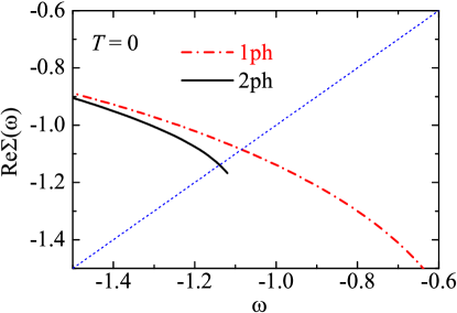
Let us first consider the zero-temperature case. At , one advantage is that the attractive polaron is the unique ground-state of the quantum many-body system, so the excitation energies and at . Thus, there is no singularity in the coupled equations for the attractive polaron branch. We do not need to introduce the small broadening factor . In Fig. 9, we show the polaron self-energy ) at zero momentum , calculated with the inclusion of one-particle-hole (1ph) and two-particle-hole (2ph) excitations, strictly at . We find with 2ph excitations, which is slightly smaller than the prediction with 1ph excitations, as expected. We note that, at the numerical calculations with 2ph excitations have to stop at a threshold energy slightly larger than , above which we encounter the zeros of and therefore our numerical procedure becomes unstable.
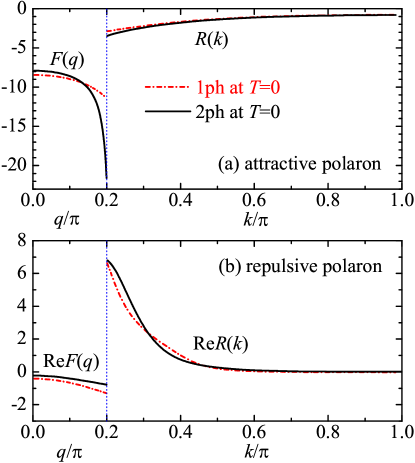
In Fig. 10, we plot the curves and , predicted with 1ph and 2ph excitations, at the attractive polaron energy (a) and at the repulsive polaron energy (b). For the latter, we must include a spectral broadening factor (i.e., ) to ensure the numerical stability, and therefore and become complex. Both and are even functions, i.e., and .
At the attractive polaron energy in Fig. 10(a), we observe that at calculated with 2ph excitations decreases very rapidly when approaches the Fermi point, . This singular behavior might be removed by either a finite broadening factor or a nonzero temperature . At the repulsive polaron energy in Fig. 10(b), we find that has a much larger magnitude than . This finding is probably not expected, since has to vanish identically in the free space with an infinitesimal interaction strength .
VI.2.2 and at nonzero temperature
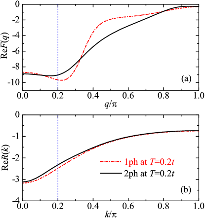
Let us now turn to investigate the finite-temperature polaron spectral function. In this case, the range of and in the functions and extends to the whole Brillouin zone , as given in Fig. 11, for the attractive Fermi polaron at with a broadening factor . For in Fig. 11(a), we find a large difference in the predictions with 1ph and 2ph excitations, at . However, this difference may not lead to too much difference in the calculated self-energy , due to the existence of the thermal weighting factor of the Fermi distribution function , see, for example, Eq. (51).
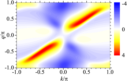
To understand why we obtain a very different with and without 2ph excitations, in Fig. 12 we show a contour plot of the corresponding , which measures the importance of the 2ph functions and . In contrast to and , has an odd parity. Therefore, at the origin and , is strictly zero. We find that is a rapidly varying function as a function of either and . This observation agrees with our impression that and could be a very singular function due to the smallness of the excitation energy . We also find that has a large magnitude roughly along the diagonal direction , peaking at about . As is an input to Eq. (53) and Eq. (54), the existence of these peaks may qualitatively explain why the calculated with and without 2ph excitations show a large difference.
VI.2.3 The -dependence of the polaron self-energy
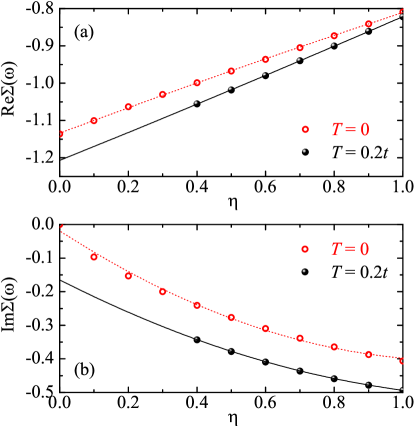
Before we present the results on the -independent polaron self-energy and spectral function, it is useful to carefully check our extrapolating strategy of a quadratic curve fitting. In Fig. 13, we report the self-energy as a function of the broadening factor at zero temperature (empty red circles) and at (black solid circles), at the attractive polaron energy. The zero-temperature results extend all the way down to , due to the nonzero excitation energy as we mentioned earlier. In contrast, at nonzero temperature, our choice of the discretization grid for momentum (i.e., used for the -point gaussian quadrature integral) only allows us to accurately calculate the self-energy with .
We observe that the results of the self-energy over a wide range of can be well fitted by using a polynomial of degree two, at both zero temperature and nonzero temperature. The fitting is particularly accurate for the real part of the self-energy, with an absolute error less than (see Fig. 13(a)). For the imaginary part of the self-energy in Fig. 13(b), we roughly estimate that the absolute error of , extrapolating to , would be around a few percent of .
VI.2.4 The polaron self-energy and spectral function
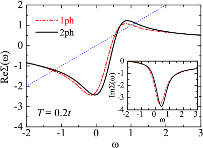
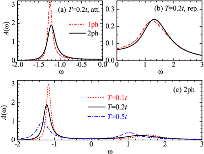
In Fig. 14, we show the polaron self-energy at , obtained by extrapolating to zero, with the inclusion of 1ph excitations (red dot-dashed lines) and 2ph excitations (black solid lines). The corresponding polaron spectral function is shown in Fig. 15(a) and Fig. 15(b), for the attractive polaron branch and the repulsive polaron branch, respectively. It is readily seen that, at nonzero temperature the attractive polaron energy predicted with 2ph excitations (at ) is slightly larger than the energy obtained with 1ph excitations (at ). Therefore, the inclusion of more particle-hole excitations does not necessarily make the attractive polaron energy smaller, as we may naïvely anticipate from the viewpoint that Chevy ansatz is a variational theory. As we mentioned earlier, this is because, at nonzero temperature the attractive Fermi polaron should be viewed as a collection of some many-body states, with different weights. In our calculations with 2ph excitations, although the energies of these (individual) many-body states become smaller due to the enlarged Hilbert space, their weights are re-distributed. Roughly, the energy of the many-body state with the maximum weight may then increase, leading to the increase in the “averaged” attractive polaron energy. On the other hand, we also find that the inclusion of 2ph excitations enlarges the decay rate or the width of the attractive polaron. As the consequence, the peak height of the attractive polaron decreases significantly in the presence of 2ph excitations.
In Fig. 15(c), we focus on the 2ph calculations and investigate the temperature dependence of the polaron spectral function. As the temperature increase, the energies of both attractive polaron and repulsive polaron become smaller. For the attractive polaron, the decay rate increases with temperature, so the peak height decreases. In contrast, the peak height of the repulsive polaron shows a non-monotonic dependence as a function of the temperature. It initially decreases slightly at low temperature and then increases with increasing temperature.
VII Conclusions and outlooks
In conclusions, we have developed an exact theory of the spectral function of Fermi polarons at finite temperature, by finding the complete set of Feynman diagrams for the multi-particle vertex functions that describe the multi-particle-hole excitations of the shake-up Fermi sea. This is a rare case of quantum many-body theories, where the exact solution is obtained by exhausting all the possible Feynman diagrams for various vertex functions.
To understand why such an exact solution is feasible, we have provided an alternative derivation, by generalizing the celebrated Chevy ansatz to the finite temperature, with the inclusion of arbitrary numbers of particle-hole excitations. We show that the ability to find an exact solution roots in the closure of the Hilbert space for available quantum states, in the case of a single impurity.
We have rigorously prove that, for an infinitesimal interaction strength in two-dimensional or three-dimensional free space, the diagrammatic theory is fully equivalent to the Chevy ansatz approach, to any orders of particle-hole excitations. In particular, the on-shell multi-particle vertex functions are precisely the variational coefficients in the Chevy ansatz. This remarkable relationship may provide a useful way to calculate the multi-particle vertex functions, which are known to be notoriously difficult to obtain in quantum many-body theories.
We have also shown that, to calculate the finite-temperature spectral function of Fermi polarons for a nonzero interaction strength, the Chevy ansatz is more powerful than the diagrammatic theory. In the latter, the nonzero interaction strength leads to infinitely many Feynman diagrams, whose roles are to be investigated in future studies.
To demonstrate the effects of multi-particle-hole excitations on the finite-temperature spectral function, we have considered a specific example of Fermi polarons in one-dimensional lattices, where the instability of numerical calculations can be effectively removed. We have shown that, for the attractive Fermi polaron at nonzero temperature, the inclusion of two-particle-hole excitations typically leads to a larger attractive polaron energy and a larger polaron decay rate. We have explained that the larger polaron energy at finite temperature does not contradict with the fact that the Chevy ansatz is a variational approach for an individual quantum many-body state. However, the variational viewpoint of the Chevy ansatz may not be worth emphasizing at nonzero temperature, where the polaron state should be treated as a collection of a number of quantum many-body states.
Our work can be straightforwardly generalized to handle the molecule state of Fermi polarons, which is the ground state when the inter-particle attraction becomes strong enough (Punk2009, ; Mora2009, ; Combescot2009, ). In Appendix C, we list the set of equations for molecules, obtained by using the Chevy ansatz approach. The parallel diagrammatic theory will be described elsewhere.
In future studies, our work might be easily generalized to address some long-standing problems in the polaron physics. The most interesting example could be the polaron-polaron interaction (Baroni2024, ). As we have emphasized, the closure of the Hilbert space for available quantum states plays an important role to obtain the exact solution. This closure of the Hilbert space should also hold for few impurities. We should then be able to write down the generalized Chevy ansatz for few impurities, in particular, for just two impurities. We may also construct Feynman diagrams for the related multi-particle vertex functions. In this way, we might be able to characterize the effective polaron-polaron interaction, which is important to understand the instability of a Fermi liquid of Fermi polarons at large impurity concentration.
In addition, our approach could also be straightforwardly generalized to investigate the spectral function of Bose polarons (Scazza2022, ; Hu2016, ) or crossover polarons (Hu2022a, ) at finite temperature, where the many-body environment is taken to be a weakly-interacting Bose gas or a strongly interacting Fermi superfluid, respectively. In these cases, special attention should be paid to the emergent three-body bound states and the related three-body parameters. The possible construction of relevant Feynman diagrams may provide insight to develop novel strong-coupling theories for strongly correlated Fermi or Bose systems.
Acknowledgements.
This research was supported by the Australian Research Council’s (ARC) Discovery Program, Grants Nos. DP240101590 (H.H.), FT230100229 (J.W.), and DP240100248 (X.-J.L.).Appendix A The antisymmetrization of
Here, we wish to show that the following function is antisymmetric with respect to the exchange of any two momenta in the set ():
| (79) |
where the function itself is already an antisymmetric function of its arguments.
Let us suppose that we exchange the two arguments and in , where and . If the -th sub-term involve both and , then it is already antisymmetrized. Thus, we only need to consider two sub-terms,
| (80) | |||||
| (81) |
Upon the exchange of the two arguments and , in the argument becomes and we need to transport this all the way backward to the position . During this transportation, a sign appears due to the antisymmetrization of the function . Therefore, we obtain . In , the argument becomes and similarly we need to transport this all the way forward to the position . As a result, . Therefore, we conclude
| (82) |
Putting all the sub-terms together, we observe that is indeed an antisymmetric function.
In Eq. (79), let us take and , we see immediately that . Hence, is an antisymmetric function upon the exchange of any two momenta in ().
Appendix B Two rules on the Matsubara frequency summation
In this appendix, we establish the two rules on the Matsubara frequency summation. Let us first consider the second rule Eq. (15), and apply it to the vertex function or its cousin , as an example.
Roughly speaking, the vertex function represents the Green function of a molecule, i.e., a quasi-bound state of two fermions with unlike spin (i.e., a spin-up fermion and the impurity). The vertex function does not have singularity at negative energy, if the molecular state is not the ground state, a situation that we will focus on. would have the similar behavior. Let us write down in its spectral representation, for example (),
| (83) |
A summation over the Matsubara frequency leads to the density of molecules, , which should be vanishingly small in the thermodynamic limit. Here, is the Fermi-Dirac distribution function. We do not worry about the negative energy, since is analytic on the half-plane , so its imaginary part vanishes there. However, on the other half-plane , the vanishing density means we should view the Fermi distribution function as an infinitesimal, i.e., , where is the volume of the whole system.
Let us now explicitly integrate out the Matsubara frequency in the expression for the self-energy, Eq. (11),
| (84) | |||||
| (85) | |||||
| (86) |
where in the second line we have taken as we emphasized earlier. This result can be easily recognized from the associated diagram and can be generalized as the second rule Eq. (15). The integration is for a Fermi loop that winds back a fermion line, on which the fermionic Matsubara frequency is to be summed. We can simply replace the backward Green function by a Fermi distribution function with an on-shell energy , where is the chemical potential of the Fermi sea. The energy in should also then be replaced by the on-shell value .
How about the first rule on the summation over the forward momentum , i.e., , where and may take on-shell values? This summation appears in the last term of the right-hand-side of Eq (5) and for clarity we have rename as . It is easy to see that the pole of the bare impurity Green function occurs at , where is the impurity chemical potential. Therefore, we have and is analytic on the half-plane . We would assume that for the argument , is also analytic on the half-plane and may then write in the spectral representation. By repeating the similar reasons for , we find that the vanishing density related to (i.e., the density of trimer) implies that we should take the Fermi distribution function as an infinitesimal on the half-plane , when we handle the forward, particle-like four-momentum .
Now, let us denote collectively , in which the other arguments other than are made implicit. As is analytic on the half-plane , we find that ,
| (87) | |||||
| (88) | |||||
| (89) |
where in the second line we have taken on the half-plane , on which may develop poles. Thus, for the summation over the fermionic Matsubara frequency for the particle-like momentum , we can simply replace the forward Green function by the Fermi distribution function with the on-shell energy , and then take in . This is exactly the first rule, Eq. (14).
Appendix C Chevy ansatz for molecules
For very strong attraction, Fermi polarons may become unstable and turn into tightly bound molecules that are dressed by particle-hole excitations of the Fermi sea (Punk2009, ; Mora2009, ; Combescot2009, ). Here, we would like to list the set of the equations for molecules, which can be easily derived following Sec. IV. The Chevy ansatz for molecules with momentum takes the form,
| (90) | |||||
| (91) |
where describes a thermal Fermi sea at finite temperature with fermions. We find that the coefficients satisfy the following coupled equations,
| (92) | |||||
where and is the energy of the Fermi sea with fermions.
References
- (1) A. S. Alexandrov and J. T. Devreese, Advances in Polaron Physics (Springer, New York, 2010), Vol. 159.
- (2) G. D. Mahan, Excitons in Metals: Infinite Hole Mass, Phys. Rev. 163, 612 (1967).
- (3) Gerald D. Mahan, Many-Particle Physics, 3rd ed. (Kluwer, New York, 2000).
- (4) B. Roulet, J. Gavoret, and P. Nozières, Singularities in the X-Ray Absorption and Emission of Metals. I. First-Order Parquet Calculation, Phys. Rev. 178, 1072 (1969).
- (5) P. Nozières, J. Gavoret, and B. Roulet, Singularities in the X-Ray Absorption and Emission of Metals. II. Self-Consistent Treatment of Divergences, Phys. Rev. 178, 1084 (1969).
- (6) P. Nozières and C. T. De Dominicis, Singularities in the X-Ray Absorption and Emission of Metals. III. One- Body Theory Exact Solution, Phys. Rev. 178, 1097 (1969).
- (7) Leonid S. Levitov and Hyunwoo Lee, Electron counting statistics and coherent states of electric current, J. Math. Phys. 37, 4845 (1996).
- (8) M. Knap, A. Shashi, Y. Nishida, A. Imambekov, D. A. Abanin, and E. Demler, Time-Dependent Impurity in Ultracold Fermions: Orthogonality Catastrophe and Beyond, Phys. Rev. X 2, 041020 (2012).
- (9) R. Schmidt, M. Knap, D. A. Ivanov, J.-S. You, M. Cetina, and E. Demler, Universal many-body response of heavy impurities coupled to a Fermi sea: a review of recent progress, Rep. Prog. Phys. 81, 024401 (2018).
- (10) J. Wang, X.-J. Liu, and H. Hu, Exact Quasiparticle Properties of a Heavy Polaron in BCS Fermi Superfluids, Phys. Rev. Lett. 128, 175301 (2022).
- (11) J. Wang, X.-J. Liu, and H. Hu, Heavy polarons in ultracold atomic Fermi superfluids at the BEC-BCS crossover: Formalism and applications, Phys. Rev. A 105, 043320 (2022).
- (12) J. Wang, Multidimensional spectroscopy of heavy impurities in ultracold fermions, Phys. Rev. A 107, 013305 (2023).
- (13) J. Wang, Functional determinant approach investigations of heavy impurity physics, AAPPS Bull. 33, 20 (2023).
- (14) P. Massignan, M. Zaccanti, and G. M. Bruun, Polarons, dressed molecules and itinerant ferromagnetism in ultracold Fermi gases, Rep. Prog. Phys. 77, 034401 (2014).
- (15) F. Scazza, M. Zaccanti, P. Massignan, M. M. Parish, and J. Levinsen, Repulsive Fermi and Bose Polarons in Quantum Gases, Atoms 10, 55 (2022).
- (16) A. Schirotzek, C.-H. Wu, A. Sommer, and M.W. Zwierlein, Observation of Fermi Polarons in a Tunable Fermi Liquid of Ultracold Atoms, Phys. Rev. Lett. 102, 230402 (2009).
- (17) Y. Zhang, W. Ong, I. Arakelyan, and J. E. Thomas, Polaron-to-Polaron Transitions in the Radio-Frequency Spectrum of a Quasi-Two-Dimensional Fermi Gas, Phys. Rev. Lett. 108, 235302 (2012).
- (18) Z. Yan, P. B. Patel, B. Mukherjee, R. J. Fletcher, J. Struck, and M.W. Zwierlein, Boiling a Unitary Fermi Liquid, Phys. Rev. Lett. 122, 093401 (2019).
- (19) M. Cetina, M. Jag, R. S. Lous, I. Fritsche, J. T. M.Walraven, R. Grimm, J. Levinsen, M. M. Parish, R. Schmidt, M. Knap, and E. Demler, Ultrafast many-body interferometry of impurities coupled to a Fermi sea, Science 354, 96 (2016).
- (20) F. Scazza, G. Valtolina, P. Massignan, A. Recati, A. Amico, A. Burchianti, C. Fort, M. Inguscio, M. Zaccanti, and G. Roati, Repulsive Fermi Polarons in a Resonant Mixture of Ultracold 6Li Atoms, Phys. Rev. Lett. 118, 083602 (2017).
- (21) F. J. Vivanco, A. Schuckert, S. Huang, G. L. Schumacher, G. G. T. Assumpção, Y. Ji, J. Chen, M. Knap, and Nir Navon, The strongly driven Fermi polaron, arXiv:2308.05746.
- (22) G. Ness, C. Shkedrov, Y. Florshaim, O. K. Diessel, J. von Milczewski, R. Schmidt, and Y. Sagi, Observation of a Smooth Polaron-Molecule Transition in a Degenerate Fermi Gas, Phys. Rev. X 10, 041019 (2020).
- (23) Y. Nagaoka, Ferromagnetism in a Narrow, Almost Half-Filled Band, Phys. Rev. 147, 392 (1966).
- (24) B. S. Shastry, H. R. Krishnamurthy, and P. W. Anderson, Instability of the Nagaoka ferromagnetic state of the Hubbard model, Phys. Rev. B 41, 2375 (1990).
- (25) A. G. Basile and V. Elser, Stability of the ferromagnetic state with respect to a single spin flip: Variational calculations for the Hubbard model on the square lattice, Phys. Rev. B 41, 4842(R) (1990).
- (26) W. von der Linden and D. M. Edwards, Ferromagnetism in the Hubbard model, J. Phys.: Condens. Matter 3, 4917 (1991).
- (27) X. Cui and H. Zhai, Stability of a fully magnetized ferromagnetic state in repulsively interacting ultracold Fermi gases, Phys. Rev. A 81, 041602(R) (2010).
- (28) F. Chevy, Universal phase diagram of a strongly interacting Fermi gas with unbalanced spin populations, Phys. Rev. A 74, 063628 (2006).
- (29) R. Combescot and S. Giraud, Normal State of Highly Polarized Fermi Gases: Full Many-Body Treatment, Phys. Rev. Lett. 101, 050404 (2008).
- (30) S. Giraud, Contribution à la théorie des gaz de fermions ultrafroids fortement polarisés (PhD Thesis 2010).
- (31) M. M. Parish and J. Levinsen, Highly polarized Fermi gases in two dimensions, Phys. Rev. A 87, 033616 (2013).
- (32) W. E. Liu, J. Levinsen, and M. M. Parish, Variational Approach for Impurity Dynamics at Finite Temperature, Phys. Rev. Lett. 122, 205301 (2019).
- (33) R. Liu, C. Peng, and X. Cui, Emergence of crystalline few-body correlations in mass-imbalanced Fermi polarons, Cell Reports Physical Science 3, 100993 (2022).
- (34) N. Prokof’ev and B. Svistunov, Fermi-polaron problem: Diagrammatic Monte Carlo method for divergent sign-alternating series, Phys. Rev. B 77, 020408(R) (2008).
- (35) R. Pessoa, S. A. Vitiello, and L. A. Peña Ardila, Finite-range effects in the unitary Fermi polaron, Phys. Rev. A 104, 043313 (2021).
- (36) R. Combescot, A. Recati, C. Lobo, and F. Chevy, Normal State of Highly Polarized Fermi Gases: Simple Many-Body Approaches, Phys. Rev. Lett. 98, 180402 (2007).
- (37) H. Hu, B. C. Mulkerin, J. Wang, and X.-J. Liu, Attractive Fermi polarons at nonzero temperatures with a finite impurity concentration, Phys. Rev. A 98, 013626 (2018).
- (38) H. Tajima and S. Uchino, Many Fermi polarons at nonzero temperature, New J. Phys. 20, 073048 (2018).
- (39) B. C. Mulkerin, X.-J. Liu, and Hui Hu, Breakdown of the Fermi polaron description near Fermi degeneracy at unitarity, Ann. Phys. (N. Y.) 407, 29 (2019).
- (40) H. Tajima and S. Uchino, Thermal crossover, transition, and coexistence in Fermi polaronic spectroscopies, Phys. Rev. A 99, 063606 (2019).
- (41) H. Hu, J. Wang, J. Zhou, and X.-J. Liu, Crossover polarons in a strongly interacting Fermi superfluid, Phys. Rev. A 105, 023317 (2022).
- (42) H. Hu and X.-J. Liu, Fermi polarons at finite temperature: Spectral function and rf spectroscopy, Phys. Rev. A 105, 043303 (2022).
- (43) H. Hu and X.-J. Liu, Raman spectroscopy of Fermi polarons, Phys. Rev. A 106, 063306 (2022).
- (44) H. Hu, J. Wang. and X.-J. Liu, Thermally stable -wave repulsive Fermi polaron without a two-body bound state, AAPPS Bull. 33, 27 (2023).
- (45) H. Hu and X.-J. Liu, Fermi spin polaron and dissipative Fermi-polaron Rabi dynamics, Phys. Rev. A 108, 063312 (2023).
- (46) R. Schmidt and T. Enss, Excitation spectra and rf response near the polaron-to-molecule transition from the functional renormalization group, Phys. Rev. A 83, 063620 (2011).
- (47) J. von Milczewski and R. Schmidt, Momentum-dependent quasiparticle properties of the Fermi polaron from the functional renormalization group, arXiv:2312.05318.
- (48) O. Goulko, A. S. Mishchenko, N. Prokof’ev, and B. Svistunov, Dark continuum in the spectral function of the resonant Fermi polaron, Phys. Rev. A 94, 051605(R) (2016).
- (49) H. Hu, J. Wang, and X.-J. Liu, Theory of the spectral function of Fermi polarons at finite temperature, arXiv:2402.11805.
- (50) H. Hu, X.-J. Liu, and P. D. Drummond, Equation of state of a superfluid Fermi gas in the BCS-BEC crossover, Europhys. Lett. 74, 574 (2006).
- (51) L. He, H. Lü, G. Cao, H. Hu, and X.-J. Liu, Quantum fluctuations in the BCS-BEC crossover of two-dimensional Fermi gases, Phys. Rev. A 92, 023620 (2015).
- (52) A. A. Abrikosov, L. P. Gorkov, and I. E. Dzyaloshinski, Methods of Quantum Field Theory in Statistical Physics (Dover, New York, 1975).
- (53) M. Punk, P. T. Dumitrescu, and W. Zwerger, Polaron-to-molecule transition in a strongly imbalanced Fermi gas, Phys. Rev. A 80, 053605 (2009).
- (54) C. Mora and F. Chevy, Ground state of a tightly bound composite dimer immersed in a Fermi sea, Phys. Rev. A 80, 033607 (2009).
- (55) R. Combescot, S. Giraud, and X. Leyronas, Analytical theory of the dressed bound state in highly polarized Fermi gases, Europhys. Lett. 88, 60007 (2009).
- (56) C. Baroni, B. Huang, I. Fritsche, E. Dobler, G. Anich, E. Kirilov, R. Grimm, M. A. Bastarrachea-Magnani, P. Massignan, and G. Bruun, Mediated interactions between Fermi polarons and the role of impurity quantum statistics, Nat. Phys. 20, 68 (2024).
- (57) M.-G. Hu, M. J. Van de Graaff, D. Kedar, J. P. Corson, E. A. Cornell, and D. S. Jin, Bose Polarons in the Strongly Interacting Regime, Phys. Rev. Lett. 117, 055301 (2016).