Building-block flow model for computational fluids

Abstract

We introduce a closure model for computational fluid dynamics, referred to as the Building-block Flow Model (BFM). The foundation of the model rests on the premise that a finite collection of simple flows encapsulates the essential physics necessary to predict more complex scenarios. The BFM is implemented using artificial neural networks and introduces five unique advancements within the framework of large-eddy simulation: (1) It is designed to predict multiple flow regimes (wall turbulence under zero, favorable, adverse mean-pressure-gradient, and separation); (2) It unifies the closure model at solid boundaries (i.e., the wall model) and the rest of the flow (i.e., the subgrid-scale model) into a single entity; (3) It ensures consistency with numerical schemes and gridding strategy by accounting for numerical errors; (4) It is directly applicable to arbitrary complex geometries; (5) It can be scaled up to model additional flow physics in the future if needed (e.g., shockwaves and laminar-to-turbulent transition). The BFM is utilized to predict key quantities of interest in turbulent channel flows, a Gaussian bump, and an aircraft in a landing configuration. In all cases, the BFM demonstrates similar or superior capabilities in terms of accuracy and computational efficiency compared to previous state-of-the-art closure models.

1 Introduction

The adoption of transformative low-emissions aero/hydro vehicle designs and propulsion systems is significantly impeded by a major obstacle: the lengthy and expensive experimental campaigns needed throughout the design cycle. These campaigns can span years and cost billions of dollars [1]. Virtual testing via computational fluid dynamics (CFD) might accelerate the process and alleviate costs [2]. However, current CFD closure models do not comply with the stringent accuracy requirements demanded by the aerospace industry [3]. These limitations primarily stem from the challenging nature of turbulence, i.e., the chaotic and multiscale motion of flows, resulting in complex physical phenomena.

Despite the challenges, novel modeling strategies hold the potential to unlock substantial financial benefits worldwide, extending far beyond the aerospace industry. The use of highly accurate CFD tools can facilitate the creation of innovative vehicle designs that achieve up to 30% fuel savings [4]. This breakthrough would result in substantial cost reductions, amounting to hundreds of billions of dollars per year within the transportation sector alone. For instance, the global ocean shipping industry consumes approximately 2 billion barrels of oil annually [5]. Similarly, the airline and trucking industries consume approximately 1.5 billion barrels and 1.2 billion barrels of oil per year, respectively. Additionally, a mere 5% reduction in transportation drag is estimated to have an impact equivalent to doubling the current wind energy production in the United States [5]. The implementation of novel turbulence modeling techniques also carries immense potential for mitigating environmental issues and reducing pollutant emissions [6].

In terms of prediction and control, the field of CFD is in the privileged position of having a highly accurate framework to model flows: the Navier–Stokes equations. However, the number of degrees of freedom involved in real-world applications ranges between $10^{13}$ to $10^{20}$, making the direct numerical simulation of all flow scales infeasible. Consequently, the treatment of turbulence in industrial CFD has primarily relied on closure models for the Reynolds-averaged Navier-Stokes (RANS) equations [7]. The approach has materialized in various forms, from pure RANS solutions to hybrid methods such as Detached Eddy Simulation and its variants [8]. Many RANS models have been developed to overcome the limitations of their predecessors, often by expanding and calibrating their coefficients to account for missing physics. However, no practical model is universally applicable across the broad range of flow regimes of interest to the industry. Examples of challenging flow scenarios include separated flows, favorable/adverse pressure gradient effects, shock waves, mean-flow three-dimensionality, and transition to turbulence, among others, as illustrated in Fig. 1(left). In these situations, RANS predictions tend to be inconsistent and unreliable, especially for geometries and conditions representative of the flight envelope of commercial airplanes [9]. Further CFD experience with aircraft at high angles of attack has revealed that RANS-based solvers have difficulties predicting maximum lift and the physical mechanisms for stall [10]. As a result, the number of wind tunnel experiments required during the final stage of the aircraft design cycle has remained at around ten for the past two decades (Fig. 1 right).

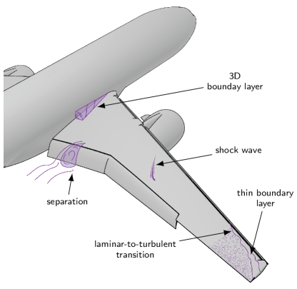
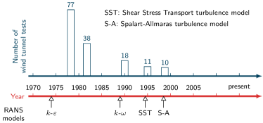
Figure 1: (Left) Schematic of the different flow phenomena encountered over an aircraft challenging current CFD methodologies. For compactness, all the phenomena are overlaid in the schematic; however, not all of them occur concurrently or even take place at all. (Right) Number of wind tunnel tests required during the design cycle as a function of time. The horizontal axis also marks the introduction of widely used RANS models. The graph is adapted from ref.[11].

Recently, large-eddy simulation (LES) has gained momentum as a tool for both scientific investigations and industrial applications. In LES, the large flow motions containing most of the energy are directly resolved by the grid, while the dissipative effect of the small scales is modeled through a subgrid-scale (SGS) model. By additionally modeling the near-wall flow using a so-called wall model, the grid-point requirements for wall-modeled LES (WMLES) scale at most linearly with increasing Reynolds number [12, 13, 14], defined as the ratio between the largest and smallest flow scales in the problem. Most widely used SGS models were developed from the 1980s to the early 2000s and are based on the eddy-viscosity assumption [15]. Among the most prominent SGS models, we can cite the similarity model [16], Vreman model [17], dynamic Smagorinsky model [18], deconvolution model [19], and sigma model [20], to name a few. A detailed account of SGS models can be found in ref.[21]. Regarding wall modeling, several strategies have been explored in the literature, and comprehensive reviews can be found in refs. [22, 23, 8, 24, 25]. A widely adopted method for wall modeling is the wall-flux approach. This approach substitutes the no-slip and thermal boundary conditions at the wall with the shear stress and heat flux values provided by the wall model. Popular examples of these approaches include those based on the law of the wall [26, 27, 28], the full/simplified RANS equations [29, 30, 31, 32, 33, 34, 35], vortex-based models [36], or dynamic wall models [37, 38].

In this context, machine learning (ML) has emerged as a powerful tool to enhance existing turbulence modeling approaches in the fluid community[39, 40, 41, 42, 43, 44]. Over the last two decades, there have been multiple efforts devoted to the development of SGS and wall models using ML tools. Most ML-based SGS models rely on supervised learning, which involves the discovery of a function that maps an input to an output based on provided training input-output pairs. Early approaches used artificial neural networks (ANNs) to emulate and speed up conventional, yet computationally expensive, SGS models[45]. More recently, SGS models have been trained to predict the so-called perfect SGS terms using data from filtered direct numerical simulation (DNS)[46, 47, 48]. Other approaches involve deriving SGS terms from optimal estimator theory[49] and deconvolution operators[50, 51, 52], as well as from reinforcement learning[53]. Similar ML methods have been employed to devise wall models for LES via supervised learning. One of the initial attempts can be found in ref. [54]. Other examples include spanwise rotating channel flows[55], flows over periodic hills[56], turbulent flows with separation[57], and boundary layer flows in the presence of shock-boundary layer interaction[58], with mixed results in a-posteriori testing. Recent works have also leveraged semi-supervised learning to devise wall models[59], although these approaches are still limited to simple flow configurations.

Despite the progress made, ML-based SGS and wall models still face challenges and have yet to serve as an effective solution for addressing long-standing issues in turbulence modeling for CFD. Even two decades after the introduction of the first ML-based SGS model for LES[45], there has been only a single demonstration of an ML-based SGS model applied to a realistic aircraft configuration. This demonstration was conducted using a prototype of the model presented here[60]. The goal of this study is to introduce a novel, unified SGS and wall model for WMLES, aiming to bridge the gap between our current predictive capabilities and the demanding requirements of the aerospace industry.

2 Results

2.1 The building-block flow model

The simulation of turbulent flows involves solving the equations for conservation of momentum:

$$\frac{\partial\rho u_{i}}{\partial t}+\frac{\partial\rho u_{i}u_{j}}{\partial x_{j}}=-\frac{\partial p}{\partial x_{i}}+\frac{\partial\sigma_{ij}}{\partial x_{j}},\ i=1,2,3,$$ (1)

along with the conservation of mass, energy, and the equation of state for the gas. Here, $\rho$ represents the flow density, $u_{i}$ denotes the $i$-th velocity component, $p$ signifies the pressure, and $\sigma_{ij}$ stands for the viscous stress tensor. Note that repeated indices in Eq. (1) imply summation. The challenge arises in numerically solving the equations on a computational grid with the ability to capture the smallest scales of the problem. In most realistic scenarios, this task becomes computationally intractable due to the hundreds of billions of grid points required. Typically, affordable grids comprise of the order of hundred million points. However, the latter grids fall short in capturing the smallest flow motions that significantly contribute to the mean forces on the vehicle. The solution lies in introducing a correction term to the right-hand side of Eq. (1), denoted as $\partial\tau^{\mathrm{SGS}}_{ij}/\partial x_{j}$, where $\tau^{\mathrm{SGS}}_{ij}$ is the SGS closure model. This corrective term accounts for the physics of the small scales unresolved by the coarse grid.

The Building-block Flow Model (BFM) provides the SGS tensor, $\tau^{\mathrm{SGS}}_{ij}$ that tackles the challenge posed by missing scales at both solid boundaries (traditionally addressed with a wall model) and in the flow above these boundaries (traditionally modeled with an SGS model). An overview of the model is shown in Fig. 2. The core modeling assumption is that the physics of the missing scales in complex scenarios can be locally mapped onto the small scales of simpler flows [60, 66]. Under this premise, it is postulated that there is a finite set of simple flows, referred to as building-block flows (BBFs), containing the essential flow physics necessary to formulate generalizable SGS and wall models. In the following, we discuss the key components of the BFM: BBFs, model architecture, and training data.

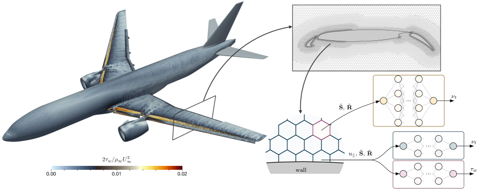
Figure 2: Schematic of the BFM applied to an aircraft in landing configuration. The tail of the aircraft is included in the model just for illustration purposes. The color over the surface of the aircraft represents the magnitude of the wall-shear stress normalized by the freestream velocity and density. The panel displays a cross-section of the grid close to the solid boundary, illustrating the three ANNs that constitute the BFM, along with their respective inputs and outputs.

2.2 Building block flows

The BBFs offer simple representations of different flow regimes for which scale-resolving, high-fidelity DNS data is available. The configuration of the BBFs entails an incompressible turbulent flow confined between two parallel walls. Four types of BBFs are considered: wall-bounded turbulence under separation, adverse, zero, and favorable mean pressure gradient. Examples of these BBFs are illustrated in Fig. 3. The intentional exclusion of cases with additional complexities, such as airfoils, wings, bumps, etc., is grounded in the idea that the BBFs should encapsulate fundamental flow physics to predict more intricate scenarios. Hence, the aim is to avoid case overfitting, e.g., correctly predicting the flow over a wing merely because the model was trained on similar wings. Note that the largest scales of the flow are intended to be resolved by the computational grid, whereas the BBFs represent the smaller flow features. This justifies the geometric simplicity of the BBFs over more complex geometries. Additionally, the computational affordability of the BBFs allows for the collection of a large number of high-fidelity simulations for training, which facilitates efficient exploration of multiple flow regimes. This aspect is important as the BFM must learn the physical scaling of the non-dimensional inputs and outputs that control the problem at hand, rather than merely fitting to a set of cases.

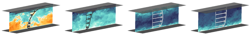
Figure 3: Examples of building-block flows (from left to right): wall-bounded turbulence under separation, adverse, zero, and favorable mean pressure gradient. The training database comprises several cases for each building block flow. Dark blue corresponds to positive streamwise velocity, and orange corresponds to negative streamwise velocity. The solid lines and arrows represent the mean velocity profile.

2.3 Model architecture

The BFM is implemented using three feedforward ANNs (see Fig. 2). The first ANN, adapted from the ML-based wall model by Lozano-Durán and Bae [66], is tasked with predicting the wall-shear stress at the solid boundaries ($\boldsymbol{\tau}_{w}$). The second ANN predicts the SGS stress tensor for control volumes adjacent to the solid boundaries, while the third ANN does the same for the remaining control volumes. The ANNs take as input the local values of the invariants of the symmetric ($\tilde{\mathbf{S}}$) and antisymmetric ($\tilde{\mathbf{R}}$) parts of the velocity gradient tensor [63]. Additionally, the first and second ANNs incorporate information about the wall-parallel velocity of the flow relative to the solid boundary ($u_{||}$). These inputs are chosen to ensure invariance under constant translations and rotations of the reference frame, along with Galilean invariance. The output of the ANNs is the value of the SGS stress tensor via the eddy viscosity $\nu_{t}$. The inputs and output variables of the first ANN are non-dimensionalized using viscous scaling (i.e., the kinematic viscosity $\nu$ and the local grid size). For the second and third ANNs, the variables are non-dimensionalized using semi-viscous scaling (based on $\nu$ and the first invariant itself). The BFM is developed for GPU architectures using the CUDA programming language, which is particularly efficient in evaluating ANNs compared to the CPU counterparts.

2.4 Training data

The training data is generated using a novel method that incorporates an ‘exact-for-the-mean’ SGS/wall model. The approach, referred to as E-WMLES, involves conducting WMLES with a control mechanism that identifies the required SGS tensor to predict specific mean statistics of interest in the flow. The statistics considered here are the mean velocity profiles and the mean wall-shear stress, which are obtained from high-fidelity data of the BBFs. The BBFs were simulated using E-WMLES in the same numerical flow solver and grid strategies subsequently employed for implementing the BFM. The data generated from these simulations were used to train the BFM, ensuring consistency between the model and the numerical schemes of the flow solver.

The E-WMLES approach diverges from the standard practice within the community of training SGS models using filtered or coarse-grained high-fidelity data. Our preference for the E-WMLES approach arises from the known fact that the SGS tensor in WMLES is not consistent with the filtered terms derived from the Navier-Stokes equations [69, 70, 71, 72]. This limitation is particularly significant in external aerodynamics applications, where the typical grid sizes used in WMLES are orders of magnitude ($10^{2}$ to $10^{4}$) coarser than the smallest length scale of the flow. In these situations, numerical errors become comparable to modeling errors, and both must be accounted for by the SGS and wall model to yield accurate predictions.

2.5 Validation cases

We validate the performance of the BFM in three cases: a turbulent channel flow, the separated flow over a bump, and an aircraft in landing configuration. The results are compared with simulations using established SGS and wall models conducted using identical meshes as those for the BFM. The models for comparison are the dynamic Smagorisky SGS model (DSM) [18, 62] or Vreman SGS model (VRE) [17] combined with the equilibrium wall model (EQ) [33]. The models are labeled as DSM-EQ and VRE-EQ, respectively. In the validation cases below, the computational cost of conducting WMLES with BFM is approximately 0.9 times that of DSM-EQ and 1.1 times that of VRE-EQ.

2.6 Turbulent channel flow

The first validation case is a turbulent channel flow, a canonical configuration in which the flow is confined between two parallel walls, as depicted by one of the BBFs in Fig. 3. This case is used to show the robustness of the BFM across Reynolds numbers and grid resolutions. The friction Reynolds numbers considered are Re${}_{\tau}=u_{\tau}h/\nu\approx 2000$ and $4200$, where $u_{\tau}$ is the friction velocity, $h$ is the channel half-height, and $\nu$ is the kinematic viscosity. The channel is driven by a streamwise pressure gradient, such that Re${}_{c}=U_{c}h/\nu=48500$ and $112500$, respectively, with $U_{c}$ representing the mean streamwise velocity at the centerline of the channel. Three spatially isotropic grid resolutions are tested: $\Delta=0.05h$, $0.1$ and $0.2h$. The BFM predicts the mean velocity profile (Fig. 4) and the mean wall-shear stress within an accuracy of 1% to 6% for the Re_τ and grid resolutions considered.

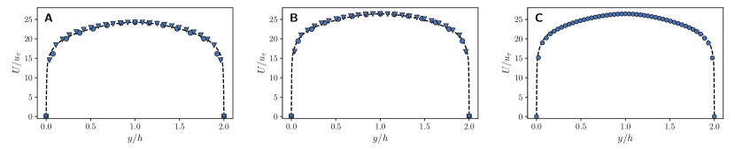
Figure 4: The mean velocity profile in a turbulent channel flow as a function of the wall-normal distance at (A) Re${}_{\tau}\approx 2000$ for grid sizes $\Delta\approx 0.2h$, and $0.1h$; (B) Re${}_{\tau}\approx 4200$ for grid sizes $\Delta\approx 0.2h$ and $0.1h$; and (C) Re${}_{\tau}\approx 4200$ for $\Delta\approx 0.05h$. The dashed line is DNS data [73] and the blue symbols are the BFM. In (A) and (B) circles correspond to $\Delta\approx 0.2h$ and triangles to $\Delta\approx 0.1h$.

2.7 Separated flow over a bump

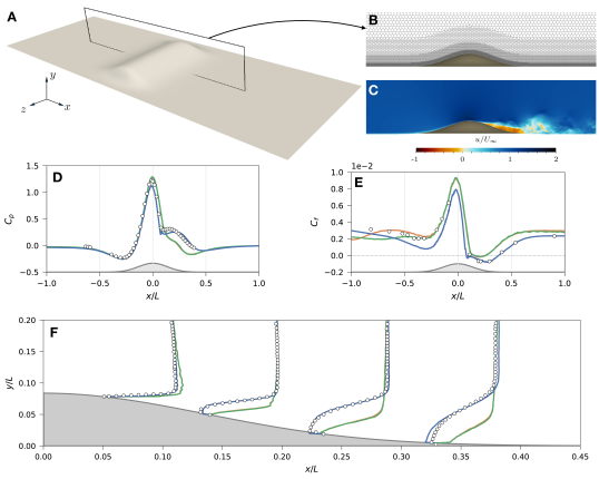
Figure 5: (A) Schematic of the Gaussian bump; (B) grid structure and (C) instantaneous streamwise velocity in the $y/L=0$ plane. The velocity of the freestream is $U_{\infty}$. Note that the figure does not show the whole domain in the streamwise direction. (D) Wall pressure coefficient $C_{p}=\frac{p-p_{\infty}}{\frac{1}{2}\rho_{\infty}U^{2}_{\infty}}$ and (E) wall friction coefficient $C_{f}=\frac{\tau_{w}}{\frac{1}{2}\rho_{\infty}U^{2}_{\infty}}$, along the $y/L=0$ plane, where $U_{\infty}$, $p_{\infty}$ and $\rho_{\infty}$ are the freestream velocity, pressure and density, respectively, and $p$ and $\tau_{w}$ are averaged over time. (F) Mean velocity profile at $y/L=0$ at different streamwise locations. In (D,E,F) The solid lines denote BFM (blue), DSM-EQ (green) and VRE-EQ (orange). White circles are experimental values[74].

The second validation case is a Gaussian bump designed by The Boeing Company and the University of Washington [75], as shown in Fig. 5. The test consists of a three-dimensional tapered hump at a Reynolds number of $3.6\times 10^{6}$ and a Mach number of $0.17$, based on the freestream quantities and the length of the bump $L$. This test case has proven to be highly challenging for the CFD community, with inaccurate prediction of the separation bubble and non-monotonic convergence of the solution with grid refinements[76, 77].

We evaluate the performance of the BFM in predicting the mean velocity profiles, and the mean pressure and friction at the wall (characterized by the non-dimensional coefficients $C_{p}$ and $C_{f}$, respectively). The simulation consists of roughly 9 million control volumes. Similar WMLESes are conducted using DSM-EQ and VRE-EQ. The numerical findings are compared with experimental data[74]. Figure 5(D,E) illustrates the evolution of $C_{p}$ and $C_{f}$ along the centerline of the bump ($x/L$). Notably, the BFM yields more accurate predictions of the $C_{p}$ and $C_{f}$ evolution in the separation region ($x/L>0.1$) compared to DSM-EQ and VRE-EQ, which even fail to predict flow separation. The improved predictions by the BFM also extend to the mean velocity profiles, as demonstrated in Fig. 5F. The BFM predicts mean velocity with up to 3% accuracy, whereas both DSM-EQ and VRE-EQ yield a similar result that overestimate the mean velocities by more than 30%. Nevertheless, there is still room for improvement upstream of the bump ($x/L<0$), where all models exhibit low accuracy in the prediction of $C_{f}$.

2.8 Aircraft in landing configuration

The third validation case is an aircraft in landing configuration, specifically the NASA Common Research Model High-Lift (CRM-HL). This case serves as the gold standard used by the aerospace community to assess the capabilities of different CFD methodologies [78]. The CRM-HL is a geometrically realistic aircraft that includes the bracketry associated with deployed flaps and slats, as well as a flow-through nacelle mounted on the underside of the wing (Fig. 2). The Reynolds number of the aircraft is 5.49 million based on the mean aerodynamic chord and freestream velocity, and the freestream Mach number is 0.20.

The simulations are conducted using approximately 30 million control volumes. Two angles of attack are considered: $\alpha=7.05^{\circ}$ and $19.57^{\circ}$. Figure 2 contains the model geometry, an inset of the mesh, and a visualization of the wall-shear stress predicted by BFM.

Figure 6 displays the forces acting on the aircraft, characterized by the lift ($C_{L}$), drag ($C_{D}$), and pitching moment ($C_{M}$) coefficients for BFM, DSM-EQ, and VRE-EQ, compared with experimental data [79]. For $\alpha=7.05^{\circ}$, DSM-EQ and VRE-EQ predict values of $C_{L}$ and $C_{D}$ close to experimental results. However, further analysis has shown that this accurate prediction is coincidental and due to error cancellation during the integration of total forces [80]. This is corroborated by the poorer predictions of the pitching moment by DSM-EQ and VRE-EQ. The case of $\alpha=19.57^{\circ}$ corresponds to the angle of attack of the maximum lift coefficient. DSM-EQ and VRE-EQ underpredict $C_{L}$, whereas the BFM offers improved predictions. Inspection of the sectional pressure coefficient, shown in Fig. 7, indicates that the BFM maintains the flow attached over a longer section of the wing compared to DSM-EQ and VRE-EQ, explaining the enhanced performance of the BFM. Overall, BFM yields improved predictions for the three coefficients compared to traditional models. The results are still far from satisfactory, especially for the pitching moment, and there is clear potential for further improvements. Nonetheless, it is worth noting that BFM has never ‘seen’ an aircraft-like flow or been trained in a case resembling an airfoil or a wing. This demonstrates the ability of the BFM methodology to offer predictions that go beyond simple regression.

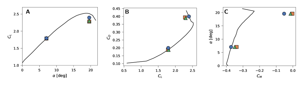
Figure 6: (A) Lift coefficient, (B) drag polar and (C) pitching moment coefficient for the CRM-HL. The black lines denote experimental results, blue circles are for the BFM, squares are for DSM-EQ and orange squared for VRE-EQ.

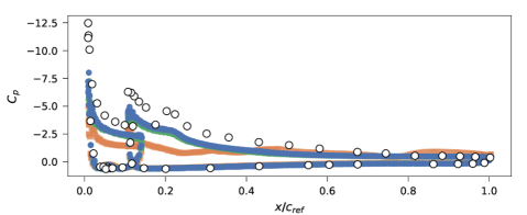
Figure 7: Pressure coefficient along the chord of the wing at the 82% spanwise section of the wing for $\alpha=19.57^{\circ}$. The chord location is normalized by the sectional chord-length $c_{\text{ref}}$. White circles represents experimental results, blue circles are for the BFM, orange and green squares are for DSM-EQ and VRE-EQ, respectively.

3 Discussion

3.1 Opportunities of BFM for CFD

The BFM has the potential to significantly advance the resolution of key Grand Challenges in the aerospace industry. These challenges include simulating an aircraft across its entire flight envelope and addressing off-design turbofan engine transients –both highlighted in the NASA CFD Vision 2030 report [3]. The BFM can also play a significant role in Certification by Analysis, i.e., the development of simulation-based methods of compliance for airplane and engine certification [1]. This marks a long-awaited milestone in the aerospace industry, with the prospect of Certification by Analysis estimated to result in substantial cost savings, amounting to billions of dollars in the design process.

A distinctive advantage of the BFM, which might contribute to addressing the aforementioned challenges compared to previous models, is its ability to accommodate various flow regimes through the BBF database. The current version of BFM includes separated flow and the effects of zero, adverse, and favorable mean pressure gradients. However, the process of incorporating additional flow physics is scalable by expanding the building block database, a capability absent in current SGS/wall models. Future versions of BFM could involve BBFs accounting for laminar flow, compressibility effects, shock waves, wall roughness, and the laminar-to-turbulent transition. Efforts to include these new physics are already underway in our group.

Finally, the machine-learning nature of the BFM also unlocks other opportunities for uncertainty quantification and adaptive grid refinement. These might be accomplished by computing a confidence score based on the similarity between the actual input data and the BFM training data. This feature has already been tested in a preliminary version of the BFM, which incorporates only a wall model[66]. The work has demonstrated that a confidence score can be determined by the distance of the input data to the closest sample in the training set. If the input data appears unusual, the model assigns a low confidence score, indicating that the flow is unfamiliar and does not align with any knowledge from the database. Regions with low confidence scores can be used to assist in automatic grid refinement in subsequent simulations, to identify the need for additional building blocks, and for uncertainty quantification.

3.2 Conclusions

We have introduced the Building-Block Flow Model (BFM) for large-eddy simulation. The model is designed to address challenges encountered in CFD within the aerospace industry, specifically the demand for accurate and robust solutions at an affordable computational cost. The core assumption of the BFM is that the subgrid-scale physics of complex flows can be effectively represented by the physics of simpler canonical flows. Implemented using three feedforward ANNs for GPU architectures, the BFM is applicable to arbitrarily complex geometries. Unlike previous models, the training data for the BFM is derived from controlled WMLES with an ‘exact’ model for the mean quantities of interest. This approach ensures consistency with the numerical discretization and grid structure of the solver. We have shown that, at the resolutions considered here, the BFM offers improvements in predictions over conventional SGS and wall models in both simple and complex scenarios.

Truly revolutionary improvements in WMLES will encompass advancements in numerics, grid generation, and wall/SGS modeling. The BFM addresses all these aspects by devising SGS/wall models consistent with the numerics and the grid. The modularity of the BFM opens up new opportunities for developing SGS/wall models that have broad applicability across different scenarios. In essence, the BFM offers a single model that can accurately represent various flow physics, eliminating the need for multiple specialized models for specific flow types. To enhance model performance, we will continue the training of future versions of the BFM with additional building blocks to account for a richer collection of flow physics.

Acknowledgments

This work was supported by the National Science Foundation under grant #2317254 and by an Early Career Faculty grant from NASA’s Space Technology Research Grants Program (grant #80NSSC23K1498). S. C was supported by The Boeing Company. G. A. was partially supported by the NNSA Predictive Science Academic Alliance Program (PSAAP; grant DE-NA0003993). The authors acknowledge the support of the CTR Summer Program 2022 at Stanford University. The authors also acknowledge the Massachusetts Institute of Technology, SuperCloud, and Lincoln Laboratory Supercomputing Center for providing HPC resources that have contributed to the research results reported here.

Author contributions

A.L.D. devised the idea and also wrote the manuscript, G.A. developed the model and wrote the manuscript, Y.L. developed and trained preliminary versions of the BFM, S.C. ported the BFM to GPU architecture, K.G. run the simulations for conventional WMLES and provided guidance on test cases and their numerical setup.

Competing interests

The authors declare no competing interests.

Appendix A Methods

A.1 Numerical solver and conventional models

The BFM provides the closure model for the SGS stress tensor $\tau_{ij}^{\mathrm{SGS}}$ for the compressible LES equations

$$\frac{\partial\bar{\rho}}{\partial t}+\frac{\partial\bar{\rho}\tilde{u}_{i}}{\partial x_{i}} = 0,$$ (2)

$$\frac{\partial\bar{\rho}\tilde{u}_{i}}{\partial t}+\frac{\partial\bar{\rho}\tilde{u}_{i}\tilde{u}_{j}}{\partial x_{j}} = -\frac{\partial\bar{p}}{\partial x_{i}}+\frac{\partial\tilde{\sigma}_{ij}}{\partial x_{j}}-\frac{\partial\tau^{\mathrm{SGS}}_{ij}}{\ \partial x_{j}},$$ (3)

$$C_{v}\frac{\partial\bar{\rho}\tilde{T}}{\partial t}+C_{v}\frac{\partial\bar{\rho}\tilde{u}_{j}\tilde{T}}{\partial x_{j}} = -\bar{p}\frac{\partial\tilde{u}_{j}}{\partial x_{j}}+\tilde{\sigma}_{ij}\frac{\partial\tilde{u}_{j}}{\partial x_{i}}$$ (4)

$$+ \frac{\partial}{\partial x_{j}}\left(\tilde{\kappa}\frac{\partial\tilde{T}}{\partial x_{j}}\right)-C_{v}\frac{\partial q^{\mathrm{SGS}}_{j}}{\partial x_{j}},$$ (5)

where repeated indices imply summation, $(\bar{\cdot})$ denotes filtered quantities, $(\tilde{\cdot})$ is the Favre average, $u_{i}$ is the $i$-th velocity component, $\rho$ is the density, $T$ is the temperature, $\kappa$ is the thermal conductivity, $C_{v}$ is the specific heat at constant volume, and $\sigma_{ij}$ is the viscous stress tensor. Note that repeated indices imply summation. The heat flux is computed as $q^{\mathrm{SGS}}_{j}=(\bar{\rho}\nu_{t}/\text{Pr})\partial\tilde{T}/\partial x_{j}$, where Pr is the turbulent Prandtl number and $\nu_{t}$ is the eddy viscosity. The applications considered in this work are low speed flow, and heat transfer and compressibility effects play no significant role.

The simulations are conducted with the solver GPU version of charLES developed by Cascade Technologies, Inc. (Cadence) [61]. The code integrates the compressible LES equations using a kinetic-energy conserving, second-order accurate, finite volume method. The numerical discretization relies on a flux formulation which is approximately entropy preserving in the inviscid limit, thereby limiting the amount of numerical dissipation added into the calculation. The time integration is performed with a third-order Runge-Kutta explicit method. The ANNs of the BFM are evaluated using the GPU capabilities of the solver.

The mesh generation follows a Voronoi hexagonal close-packed point-seeding method, which automatically builds locally isotropic meshes for arbitrarily complex geometries. First, the water-tight surface geometry is provided to describe the computational domain. Second, the coarsest grid resolution in the domain is set to uniformly seeded points. Additional refinement levels are specified in the vicinity of the walls if needed. Thirty iterations of Lloyd’s algorithm are undertaken to smooth the transition between layers with different grid resolutions.

The dynamic Smagorinsky model [18] with the modification by Lilly [62] and the Vreman model [17] are considered as SGS models. For the wall, we use an equilibrium wall model. The no-slip boundary condition at the wall is replaced by a wall-stress boundary condition. The walls are assumed adiabatic and the wall stress is obtained by an algebraic equilibrium wall model derived from the integration of the one-dimensional stress model along the wall-normal direction [28],

$$u_{||}^{+}(y_{\perp}^{+})=\begin{cases}y_{\perp}^{+}+a_{1}(y_{\perp}^{+})^{2}\text{\, \, \, for $y_{\perp}^{+}<23$},\\ \frac{1}{\kappa}\ln{y_{\perp}^{+}}+B\text{\, \, \, \, otherwise}\end{cases}$$ (6)

where $u_{||}$ is the model wall-parallel velocity at the second grid point off the wall, $y_{\perp}$ is the wall-normal direction to the surface, $\kappa=0.41$ is the Kármán constant, $B=5.2$ is the intercept constant, and $a_{1}$ is computed to ensure $C^{1}$ continuity. The superscript $+$ denotes inner units defined in terms of wall friction velocity and the kinematic viscosity.

A.2 BFM formulation

The anisotropic component of the SGS stress tensor is given by the eddy-viscosity model

$$\tau^{\text{SGS}}_{ij}=-2\nu_{t}\tilde{S}_{ij},$$ (7)

where $\tilde{S}_{ij}$ is the rate-of-strain tensor. The eddy viscosity is a function of the first five invariants ($I_{k}$) of rate-of-strain ($\mathbf{\tilde{S}}\equiv\tilde{S}_{ij}$) and rate-of-rotation tensors ($\mathbf{\tilde{R}}\equiv\tilde{R}_{ij}$) [63],

$$\nu_{t}=f(I_{1},I_{2},I_{3},I_{4},I_{5},\theta),$$ (8)

where $f$ represents a feedforward ANN, and $\theta$ denotes additional input variables, namely, $\nu$, $\Delta$ and $u_{\parallel}$, where $\nu$ is the kinematic viscosity, $\Delta$ is the characteristic grid size and $u_{\parallel}$ is the magnitude of the wall-parallel velocity measured with respect to the wall. The latter is only used by the ANNs acting on the control volumes adjacent to the walls. The invariants are defined as

$$\begin{array}[]{ccccc}I_{1}=\operatorname{tr}\left(\mathbf{\tilde{S}}^{2}\right),&I_{2}=\operatorname{tr}\left(\mathbf{\tilde{R}}^{2}\right),&I_{3}=\operatorname{tr}\left(\mathbf{\tilde{S}}^{3}\right),\\ I_{4}=\operatorname{tr}\left(\mathbf{\tilde{S}\tilde{R}}{}^{2}\right),&I_{5}=\operatorname{tr}\left(\mathbf{\tilde{S}}^{2}\mathbf{\tilde{R}}^{2}\right).\end{array}$$ (9)

The ANNs are fully-connected feedforward networks. The first ANN, tasked with predicting the wall-shear stress, consists of 6 layers with 40 neurons per layer. The second near-wall ANN consists of 10 layers with 12 neurons per each layer; and the outer-layer ANN consists of 10 layers with 16 neurons per layer. The non-dimensionalization of the input and output features is attained by using parameters that are local in both time and space to guarantee the applicability of the model to complex geometries. For the ANN responsible for predicting the wall-shear stress, the input and output quantities are non-dimensionalized using viscous scaling: $\nu$ and $\Delta$. For the ANNs predicting the eddy viscosity, the input and output variables are non-dimensionalized using semi-viscous scaling: $(\nu\sqrt{\mathbf{\tilde{S}}:\mathbf{\tilde{S}}})^{1/2}$ and $\Delta$.

A.3 Training data preparation

The mean velocity profiles and wall-shear stress are extracted from DNS data of the BBFs. The turbulent channel flows are used to model the regime where turbulence is fully developed without significant mean-pressure gradient effects. Separation, adverse and favorable mean pressure gradient effects are learned from turbulent Poiseuille-Couette (TPC) flows. In these cases, the top wall moves at a constant speed ($U_{t}$) in the streamwise direction, and a mean pressure gradient is applied in the direction opposed to the top wall velocity. The pressure gradient ranges from mild to strong, so that the flow “separates” (i.e., zero wall shear stress) on the bottom wall. Favorable mean pressure gradient effects are obtained from the upper wall of the TPC cases.

For turbulent channel flows, the mean DNS quantities are obtained from the database in refs.[64, 65]. Five cases with friction Reynolds numbers 550, 950, 2000, 4200 and 10000 are used. For the TPC flows, the data was obtained from ref.[66]. The Reynolds numbers based on the mean pressure gradient are $\mathit{Re_{P}}={\sqrt{h^{3}\mathrm{d}P/\mathrm{d}x}}/\nu=340,680$ and $962$, and the Reynolds number based on the top wall velocity is $\mathit{Re_{U}}=U_{t}h/\nu=22,360$, where $h$ is the channel half-height. The computational domain in the streamwise, wall-normal, and spanwise direction is $L_{x}\times L_{y}\times L_{z}=4\pi h\times 2h\times 2\pi h$ for channel flows and $L_{x}\times L_{y}\times L_{z}=2\pi h\times 2h\times\pi h$ for TPC cases.

To generate the training data, we perform WMLES simulations of the BBFs adjusting $\nu_{t}$ to match the mean DNS velocity profile and correct wall-shear stress using the E-WMLES approach[66]. The simulations are performed in charLES. The eddy viscosity is adjusted by finding a correcting factor $k(y)$ to a base model $\nu^{\text{base}}_{t}$ (in this case Vreman SGS model [17]),

$$\quad\nu_{t}(x,y,z,t)=\nu^{\text{base}}_{t}(x,y,z,t)k(y),$$ (10)

where $x$, $y$, and $z$ are the streamwise, wall-normal, and spanwise directions, respectively, of the BBFs. The correcting factor is in turn computed by solving the optimization problem

$$\arg\min_{k(y)}\quad\int|U^{\text{DNS}}(y)-\tilde{U}(y)|^{2}\mathrm{d}y$$ (11)

where $U^{\text{DNS}}$ is the mean velocity profile from DNS and $\tilde{U}$ is the mean velocity profile from WMLES obtained using the eddy viscosity in (10). The free Conjugate-Gradient algorithm and the Bayesian Global optimization algorithm [67] are used to minimize (11) for the turbulent channel and the TPC flows, respectively. A Dirichlet non-slip boundary condition is applied at the walls and the correct wall shear stress is enforced by augmenting the eddy viscosity at the walls such that $\left.\nu_{t}\right|_{w}=\left.\left(\partial\tilde{u}/\partial y\right)\right|_{w}^{-1}\tau_{w}/\rho-\nu$, following [68], where the subscript $w$ denotes quantities at the wall, and $\tau_{w}$ is the mean wall-shear stress. The grid size for the WMLES cases with E-WMLES is $\Delta\approx 0.1h$ and $\approx 0.2h$ for the turbulent channel flows and $\Delta\approx 0.1h$ for the TPC flows.

The optimization process for a given case is as follows: 1) WMLES simulation is performed with a fixed $\tau_{w}$ –equal to the correct value from DNS simulations, $\tau_{w}^{\text{DNS}}$– and with an initial random $k(y)$; 2) the simulation is run until the statistical steady state is reached; 3) the integral in (11) is evaluated, and 4) a new guess of $k(y)$ is provided by the optimizer. This approach is continued until the condition

$$\frac{|U^{\text{DNS}}(y)-\tilde{U}(y)|}{U^{\text{DNS}}(y)}<0.03$$

at each $y$ location for the turbulent channel flow cases is satisfied. For the TPC cases, this condition was too stringent, since velocities are close to $0$ near the wall, and we relaxed the condition to

$$\frac{|U^{\text{DNS}}(y)-\tilde{U}(y)|}{U_{t}}<0.02.$$

References

- [1] Timothy Mauery, Juan Alonso, Andrew Cary, Vincent Lee, Robert Malecki, Dimitri Mavriplis, Gorazd Medic, John Schaefer, and Jeffrey Slotnick. A guide for aircraft certification by analysis. Technical Report No. NASA/CR-20210015404., 2021.
- [2] Mori Mani and Andrew J. Dorgan. A perspective on the state of aerospace computational fluid dynamics technology. Annu. Rev. Fluid Mech., 55(1):431–457, 2023.
- [3] J. Slotnick, A. Khodadoust, J. Alonso, D. Darmofal, W. Gropp, E. Lurie, and D. Mavriplis. CFD Vision 2030 Study: A Path to Revolutionary Computational Aerosciences. Technical Report, NASA/CR-2014-218178, NF1676L-18332, 2014.
- [4] Martin M DAngelo, John Gallman, Vicki Johnson, Elena Garcia, Jimmy Tai, and Russell Young. N+3 small commercial efficient and quiet transportation for year 2030-2035. Technical Report No. NASA/CR-2010-216691, 2010.
- [5] Alexander J. Smits and Ivan Marusic. Wall-bounded turbulence. Phys. Today, 66(9):25–30, 2013.
- [6] Adam B Smith and Richard W Katz. Us billion-dollar weather and climate disasters: data sources, trends, accuracy and biases. Nat. Hazards, 67(2):387–410, 2013.
- [7] Michael. Casey, Torsten. Wintergerste, Turbulence European Research Community on Flow, and Combustion. ERCOFTAC best practice guidelines: ERCOFTAC special interest group on “quality and trust in industrial CFD”. ERCOFTAC, 2000.
- [8] P. R. Spalart. Detached-eddy simulation. Annu. Rev. Fluid Mech., 41:181–202, 2009.
- [9] Christopher L. Rumsey. The NASA Juncture Flow Test as a Model for Effective CFD/Experimental Collaboration. In 2018 Applied Aerodynamics Conference, 2018.
- [10] C. C. Kiris, A. S. Ghate, J. C. Duensing, O. M. Browne, J. A. Housman, G.-D. Stich, G. Kenway, L. S. Fernandes, and L. M. Machado. High-lift common research model: RANS, HRLES, and WMLES perspectives for CLmax prediction using LAVA. In AIAA Scitech 2022 Forum, page 1554, 2022.
- [11] H. Xiao and P. Cinnella. Quantification of model uncertainty in rans simulations: A review. Prog. Aerosp. Sci., 108:1–31, 2019.
- [12] H. Choi and P. Moin. Grid-point requirements for large eddy simulation: Chapman’s estimates revisited. Phys. Fluids, 24(1):011702, 2012.
- [13] X. I. A. Yang and K. P. Griffin. Grid-point and time-step requirements for direct numerical simulation and large-eddy simulation. Phys. Fluids, 33(1):015108, 2021.
- [14] A. Lozano-Durán, S. T. Bose, and P. Moin. Performance of wall-modeled les with boundary-layer-conforming grids for external aerodynamics. AIAA J., 60(2):747–766, 2022.
- [15] Joseph Smagorinsky. General circulation experiments with the primitive equations: I. the basic experiment. Mon. Weather Rev., 91(3):99–164, 1963.
- [16] Jorge Bardina, J Ferziger, and WC Reynolds. Improved subgrid-scale models for large-eddy simulation. In 13th Fluid and PlasmaDynamics conference, page 1357, 1980.
- [17] A. W. Vreman. An eddy-viscosity subgrid-scale model for turbulent shear flow: Algebraic theory and applications. Phys. Fluids, 16(10):3670–3681, 2004.
- [18] M. Germano, U. Piomelli, P. Moin, and W. H. Cabot. A dynamic subgrid-scale eddy viscosity model. Phys. Fluids, 3(7):1760–1765, 1991.
- [19] S. Stolz and N. A. Adams. An approximate deconvolution procedure for large-eddy simulation. Phys. Fluids, 11(7):1699–1701, 1999.
- [20] Franck Nicoud, Hubert Baya Toda, Olivier Cabrit, Sanjeeb Bose, and Jungil Lee. Using singular values to build a subgrid-scale model for large eddy simulations. Phys. Fluids, 23(8):085106, 2011.
- [21] P. Sagaut and C. Meneveau. Large Eddy Simulation for Incompressible Flows: An Introduction. Scientific Computation. Springer, 2006.
- [22] W. H. Cabot and P. Moin. Approximate wall boundary conditions in the large-eddy simulation of high Reynolds number flow. Flow Turbul. Combust., 63:269–291, 2000.
- [23] U. Piomelli and E. Balaras. Wall-layer models for large-eddy simulations. Annu. Rev. Fluid Mech., 34:349–374, 2002.
- [24] J. Larsson, S. Kawai, J. Bodart, and I. Bermejo-Moreno. Large eddy simulation with modeled wall-stress: recent progress and future directions. Mech. Eng. Rev., 3(1):1–23, 2016.
- [25] S. T. Bose and G. I. Park. Wall-modeled les for complex turbulent flows. Annu. Rev. Fluid Mech., 50(1):535–561, 2018.
- [26] J. Deardorff. A numerical study of three-dimensional turbulent channel flow at large Reynolds numbers. J. Fluid Mech., 41(1970):453–480, 1970.
- [27] U. Schumann. Subgrid scale model for finite difference simulations of turbulent flows in plane channels and annuli. J. Comp. Phys., 18:376–404, 1975.
- [28] U. Piomelli, J. Ferziger, P. Moin, and J. Kim. New approximate boundary conditions for large eddy simulations of wall-bounded flows. Phys. Fluids A, 1(6):1061–1068, 1989.
- [29] E. Balaras, C. Benocci, and U. Piomelli. Two-layer approximate boundary conditions for large-eddy simulations. AIAA J., 34(6):1111–1119, 1996.
- [30] M. Wang and P. Moin. Dynamic wall modeling for large-eddy simulation of complex turbulent flows. Phys. Fluids, 14(7):2043–2051, 2002.
- [31] D. Chung and D. I. Pullin. Large-eddy simulation and wall modelling of turbulent channel flow . J. Fluid Mech., 631:281–309, 2009.
- [32] J. Bodart and J. Larsson. Wall-modeled large eddy simulation in complex geometries with application to high-lift devices. Center for Turbulence Research - Annual Research Briefs, pages 37–48, 2011.
- [33] S. Kawai and J. Larsson. Wall-modeling in large eddy simulation: Length scales, grid resolution, and accuracy. Phys. Fluids, 24(1):015105, 2012.
- [34] G. I. Park and P. Moin. An improved dynamic non-equilibrium wall-model for large eddy simulation. Phys. Fluids, 26(1):015108, 2014.
- [35] X. I. A. Yang, J. Sadique, R. Mittal, and C. Meneveau. Integral wall model for large eddy simulations of wall-bounded turbulent flows. Phys. Fluids, 27(2):025112, 2015.
- [36] Dale I Pullin. A vortex-based model for the subgrid flux of a passive scalar. Phys. Fluids, 12(9):2311–2319, 2000.
- [37] S. T. Bose and P. Moin. A dynamic slip boundary condition for wall-modeled large-eddy simulation. Phys. Fluids, 26(1):015104, 2014.
- [38] H. J. Bae, A. Lozano-Durán, S. T. Bose, and P. Moin. Dynamic slip wall model for large-eddy simulation. J. Fluid Mech., 859:400–432, 2019.
- [39] Steven L. Brunton, Bernd R. Noack, and Petros Koumoutsakos. Machine learning for fluid mechanics. Annu. Rev. Fluid Mech., 52(1):477–508, 2020.
- [40] M.P. Brenner, J.D. Eldredge, and J.B. Freund. Perspective on machine learning for advancing fluid mechanics. Phys. Rev. Fluids, 4(10):100501, 2019.
- [41] S. Pandey, Jörg Schumacher, and K.R. Sreenivasan. A perspective on machine learning in turbulent flows. J. Turbul., 21(9-10):567–584, 2020.
- [42] A. Beck and M. Kurz. A perspective on machine learning methods in turbulence modeling. GAMM-Mitt, 44(1):e202100002, 2021.
- [43] K. Duraisamy. Perspectives on machine learning-augmented reynolds-averaged and large eddy simulation models of turbulence. Phys. Rev. Fluids, 6(5):050504, 2021.
- [44] Ricardo Vinuesa and Steven L Brunton. Enhancing computational fluid dynamics with machine learning. Nat. Comput. Sci., 2(6):358–366, 2022.
- [45] F. Sarghini, G. De Felice, and S. Santini. Neural networks based subgrid scale modeling in large eddy simulations. Comput. Fluids, 32(1):97–108, 2003.
- [46] M. Gamahara and Y. Hattori. Searching for turbulence models by artificial neural network. Phys. Rev. Fluids, 2(5):054604, 2017.
- [47] C. Xie, J. Wang, H. Li, M. Wan, and S. Chen. Artificial neural network mixed model for large eddy simulation of compressible isotropic turbulence. Phys. Fluids, 31(8):085112, 2019.
- [48] Jonghwan Park and Haecheon Choi. Toward neural-network-based large eddy simulation: application to turbulent channel flow. J. Fluid Mech., 914:A16, 2021.
- [49] A. Vollant, G. Balarac, and C. Corre. Subgrid-scale scalar flux modelling based on optimal estimation theory and machine-learning procedures. J. Turbul., 18(9):854–878, 2017.
- [50] S. Hickel, S. Franz, N. A. Adams, and P. Koumoutsakos. Optimization of an implicit subgrid-scale model for LES. In Proceedings of the 21st International Congress of Theoretical and Applied Mechanics, Warsaw, Poland, 2004.
- [51] R. Maulik and O. San. A neural network approach for the blind deconvolution of turbulent flows. J. Fluid Mech., 831:151–181, 2017.
- [52] K. Fukami, K. Fukagata, and K. Taira. Super-resolution reconstruction of turbulent flows with machine learning. J. Fluid Mech., 870:106–120, 2019.
- [53] Guido Novati, Hugues Lascombes de Laroussilhe, and Petros Koumoutsakos. Automating turbulence modelling by multi-agent reinforcement learning. Nat. Mach. Intell., 3(1):87–96, 2021.
- [54] X. Yang, S. Zafar, J.-X. Wang, and H. Xiao. Predictive large-eddy-simulation wall modeling via physics-informed neural networks. Phys. Rev. Fluids, 4(3):034602, 2019.
- [55] X. L. D. Huang, X. I. A. Yang, and R. F. Kunz. Wall-modeled large-eddy simulations of spanwise rotating turbulent channels–Comparing a physics-based approach and a data-based approach. Phys. Fluids, 31(12):125105, 2019.
- [56] Z. Zhou, G. He, and X. Yang. Wall model based on neural networks for LES of turbulent flows over periodic hills. Phys. Rev. Fluids, 6(5):054610, 2021.
- [57] R. Zangeneh. Data-driven model for improving wall-modeled large-eddy simulation of supersonic turbulent flows with separation. Phys. Fluids, 33(12):126103, 2021.
- [58] R. Bhaskaran, R. Kannan, B. Barr, and S. Priebe. Science-guided machine learning for wall-modeled large eddy simulation. In 2021 IEEE International Conference on Big Data, pages 1809–1816. IEEE, 2021.
- [59] H. J. Bae and P. Koumoutsakos. Scientific multi-agent reinforcement learning for wall-models of turbulent flows. Nat. Commun., 13(1):1443, 2022.
- [60] Y. Ling, G Arranz., E Williams., K. Goc, K. Griffin, and A. Lozano-Durán. WMLES based on building block flows. Proceedings of the Summer Program, Center for Turbulence Research , Stanford University, 2022.
- [61] G. A. Bres, S. T. Bose, M. Emory, F. E. Ham, O. T. Schmidt, G. Rigas, and T. Colonius. Large-eddy simulations of co-annular turbulent jet using a Voronoi -based mesh generation framework. In 2018 AIAA/CEAS Aeroacoustics Conference, page 3302, 2018.
- [62] D. K. Lilly. A proposed modification of the Germano subgrid-scale closure method. Phys. Fluids, 4(3):633–635, 1992.
- [63] Thomas S Lund and EA Novikov. Parameterization of subgrid-scale stress by the velocity gradient tensor. Annual Research Briefs, 1992, 1993.
- [64] A. Lozano-Durán and J. Jiménez. Effect of the computational domain on direct simulations of turbulent channels up to = 4200. Phys. Fluids, 26(1):011702, 2014.
- [65] S. Hoyas, M. Oberlack, F. Alcántara-Ávila, S. V. Kraheberger, and J. Laux. Wall turbulence at high friction Reynolds numbers. Phys. Rev. Fluids, 7:014602, 2022.
- [66] Adrián Lozano-Durán and H. Jane Bae. Machine learning building-block-flow wall model for large-eddy simulation. J. Fluid Mech., 963:A35, 2023.
- [67] Fernando N. Bayesian Optimization: Open source constrained global optimization tool for Python, 2014–.
- [68] H. J. Bae and A. Lozano-Durán. Effect of wall boundary conditions on a wall-modeled large-eddy simulation in a finite-difference framework. Fluids, 6(3):112, 2021.
- [69] T. S. Lund and H. J. Kaltenbach. Experiments with explicit filtering for LES using a finite-difference method. Center for Turbulence Research - Annual Research Briefs, pages 91–105, 1995.
- [70] T. S. Lund. The use of explicit filters in large eddy simulation. Comput. Math. App., 46(4):603–616, 2003.
- [71] H. J. Bae and A. Lozano-Durán. Towards exact subgrid-scale models for explicitly filtered large-eddy simulation of wall-bounded flows. Center for Turbulence Research - Annual Research Briefs, pages 207–214, 2017.
- [72] H. J. Bae and A. Lozano-Durán. DNS-aided explicitly filtered LES of channel flow. Center for Turbulence Research - Annual Research Briefs, pages 197–207, 2018.
- [73] A. Lozano-Durán and J. Jiménez. Effect of the computational domain on direct simulations of turbulent channels up to = 4200. Phys. Fluids, 26(1):011702, 2014.
- [74] P. D. Gray, I. Gluzman, F. O. Thomas, and T. C. Corke. Experimental Characterization of Smooth Body Flow Separation Over Wall-Mounted Gaussian Bump. In AIAA Scitech 2022 Forum, pages 1–23, 2022.
- [75] O. Williams, M. Samuell, E. S. Sarwas, M. Robbins, and A. Ferrante. Experimental study of a cfd validation test case for turbulent separated flows. In AIAA Scitech 2020 Forum, pages 1–19, 2020.
- [76] P. S. Iyer and M. R. Malik. Wall-modeled LES of flow over a Gaussian bump. In AIAA Scitech 2021 Forum, pages 1–18, 2021.
- [77] R. Agrawal, M. P. Whitmore, K. P. Griffin, S. T. Bose, and P. Moin. Non-Boussinesq subgrid-scale model with dynamic tensorial coefficients. Phys. Rev. Fluids, 7:074602, 2022.
- [78] D. S. Lacy and A. J. Sclafani. Development of the high lift common research model (hl-crm): A representative high lift configuration for transonic transports. In 54th AIAA Aerospace Sciences Meeting, page 0308, 2016.
- [79] A. N Evans, D. S. Lacy, I. Smith, and M. B. Rivers. Test summary of the nasa high-lift common research model half-span at qinetiq 5-metre pressurized low-speed wind tunnel. In AIAA AVIATION 2020 FORUM, page 2770, 2020.
- [80] K. Goc, S. T. Bose, and P. Moin. Large eddy simulation of the nasa high-lift common research model. In AIAA SCITECH 2022 Forum, page 1556, 2022.