Frequency-dependent entanglement advantage in spin-network Quantum Reservoir Computing

Abstract

We study the performance of an Ising spin network for quantum reservoir computing (QRC) in linear and non-linear memory tasks. We investigate the extent to which quantumness enhances performance by monitoring the behaviour of quantum entanglement, which we quantify by means of the partial transpose of the density matrix. In the most general case where the effects of dissipation are incorporated, our results indicate that the strength of the entanglement advantage depends on the frequency of the input signal; the benefit of entanglement is greater the more rapidly fluctuating the signal, whereas a low-frequency input lends itself better to a non-entangled reservoir. This suggests that the extent to which quantumness is beneficial is dependent on the difficulty of the memory task.

I Introduction

At the heart of machine learning lie the mechanisms that enable machines to understand, process, and act upon temporal data. The importance of these mechanisms grows rapidly as we push further into the information age, where the complexity and volume of data are scaling at unprecedented rates. Among the principal hurdles in this pursuit is the inherent limitation in processing speeds of conventional computers caused by the segregation of processing and memory units, known as the von Neumann bottleneck von Neumann [1993]. This stands in contrast with biological systems, which handle real-time information processing with exceeding computational efficiency and minimal energy expenditure Eliasmith et al. [2012], Stewart et al. [2012].
Within this landscape, the paradigm of reservoir computing (RC) Jaeger and Haas [2004], Maass et al. [2002], Verstraeten et al. [2007] emerges as a powerful mechanism, characterized by a high-dimensional dynamical structure known as a reservoir. This system, upon receiving streams of input, engenders transient dynamics featuring a fading memory capacity and the ability to perform nonlinear processing on input data. The complex internal dynamics of the reservoir render RC exceptionally well-suited for machine learning tasks that demand memory-retention capabilities, such as speech recognition, stock market prediction, and autonomous motor control for robots Tanaka et al. [2019]. Traditional approaches to RC have been based on either randomly-connected artificial neural networks or through spiking neural networks Nicola and Clopath [2017]. Physical implementations of RC have been realized with photonics Vandoorne et al. [2014], Antonik et al. [2017], Larger et al. [2017], Sunada and Uchida [2021], García-Beni et al. [2023], phonons Dion et al. [2018], Meffan et al. [2023], magnons Papp et al. [2021], Gartside et al. [2022], Körber et al. [2023], spintronics Torrejon et al. [2017], Furuta et al. [2018], Tsunegi et al. [2018], and nanomaterials structured in neuromorphic chips Stieg et al. [2011], Yaremkevich et al. [2023].

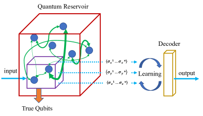
[h]

Figure 1: Schematic representation of the spin-based quantum reservoir computing. The reservoir (red box) consists of N qubits (blue circles) which are randomly connected, and stay constant. At each step, the input data is fed to only a few of the qubits, true qubits (purple box). After data feeding, the correlation of Pauli matrices, $x,y,z$ from n qubits will be measured and sent to a classical decoder. For the next iteration, the true qubits will be traced out from the density matrix. The reservoir and the decoder are linked with weights that are the only ones that get modified during the learning process.

Quantum reservoir computing (QRC) has been on the rise in recent years, introducing to RC such counter-intuitive features of quantum physics as superposition and entanglement Fujii and Nakajima [2017, 2021]. Two distinct QRC models have been proposed: one is grounded in networks of qubits Fujii and Nakajima [2021], Luchnikov et al. [2019], Martínez-Peña et al. [2020] and another in oscillator-based Govia et al. [2021], Nokkala et al. [2021], Dudas et al. [2023] reservoirs. In this work we focus on the former model. Within this type of QR, transitions of basis states for quantum bits (qubits) are propelled by an input stream (Fig. 1), evolving over time through the reservoir’s quantum dynamics Nakajima et al. [2019], Martínez-Peña et al. [2021]. Input data is fed into the true nodes, typically in the form of a time series. For the readout, besides these true nodes, hidden nodes can also be used, which influence the time evolution of the true nodes.
The primary obstacle encountered by quantum computing and quantum machine learning is the noise present in quantum devices. Significant efforts have been dedicated to correcting or mitigating the resulting errors. Recent studies show that the presence of noise can improve the convergence of variational quantum algorithms Fry et al. [2023]. Further, it is suggested that quantum noise, under specific conditions, can enhance the efficacy of quantum reservoir computing Suzuki et al. [2022b], Domingo et al. [2023].
For time-series data, the frequency and the stochasticity of the data play crucial roles in the performance of machine learning models. Time-series data, characterized by its sequential order, can vary in frequency from high-resolution milliseconds to monthly or yearly observations Abreu Araujo et al. [2020], Ballarin et al. [2023], Tanaka et al. [2019]. On the other hand, studies suggest potential advantages of quantum computing in systems characterized by high levels of stochasticity and randomness, though these advantages are not always measured against the most optimized classical solutions Dale et al. [2015], Blank et al. [2021], Korzekwa and Lostaglio [2021]. Experimental evidence tentatively indicates that quantum approaches to simulating stochastic processes might require less memory than traditional classical methods, under certain conditions Palsson et al. [2017]. Furthermore, preliminary findings propose that, by negotiating the trade-off between accuracy and memory usage, quantum models could potentially achieve comparable levels of accuracy with reduced memory requirements, or conversely, improve accuracy without increasing the memory footprint Banchi [2023]. However, these observations are context-dependent and should be considered with caution, as the comparisons are not universally applicable across all scenarios.
Beyond the inherent noise challenges, the salient aspects of quantumness —superposition and entanglement — are pivotal in understanding quantum systems. Recently, considerable research effort has been devoted to the role played by quantumness in giving rise to advantage in machine learning, whether in distributed learning over quantum networks Gilboa and McClean [2023], spin-network QRC Götting et al. [2023], or oscillator-based QRC Motamedi et al. [2023]. However, there remains much to be understood as to the physical circumstances conducing to such a quantum advantage.
Here, we conduct a thorough investigation of how the quantumness of Ising spin-networks, which we quantify by means of the logarithmic negativity measure of entanglement, relates to performance in QRC memory tasks. We explore how that relationship is affected by dissipation, of which some amount has been observed to enhance performance Domingo et al. [2023], Suzuki et al. [2022a], Götting et al. [2023]; as well as by the frequency of the input signal, which we show here has great implications for the computational advantage granted by entanglement. We find that the presence of that advantage is frequency-dependent in the presence of dissipation but is always present in the unitary reservoir. But wherever it is present, there are diminishing returns on the entanglement advantage; the positive impact of entanglement on performance exhibits saturation behavior.
The remainder of this paper is organized as follows: in section II we describe our dynamical models and methodology for data extraction and coarse-graining. We present and discuss our results in section III, and finally outline our conclusions in section IV.

II Model and Methodology

II.1 Physical System

The quantum reservoir we employ is a network of $N=4$ qubits represented by the transverse-field Ising model Stinchcombe [1973], Pfeuty and Elliott [1971], of which the Hamiltonian reads

$$\hat{H}=\sum_{i>j=1}^{N}J_{ij}\hat{\sigma}_{i}^{x}\hat{\sigma}_{j}^{x}+h\sum_{i=1}^{N}\hat{\sigma}_{i}^{z}$$ (1)

where $\hat{\sigma}_{i}^{a}$ ($a=x,y,z$) are the Pauli operators, $h$ is the transverse magnetic field, and $J_{ij}$ are randomly chosen from a uniform distribution in the interval $[-J_{s}/2,J_{s}/2]$. We consider an open system in general, of which the Markovian dynamics are given by the Lindblad master equation

$$\frac{d\hat{\rho}}{dt}=\mathcal{\hat{L}}\hat{\rho}=-i[\hat{H},\hat{\rho}]+\Gamma\sum_{i=1}^{N}\left(\hat{L}_{i}\hat{\rho}\hat{L}_{i}^{\dagger}-\frac{1}{2}\{\hat{L}_{i}^{\dagger}\hat{L}_{i},\hat{\rho}\}\right)$$ (2)

where $\Gamma$ controls the strength of the dissipation of our high-temperature decoherence channel Breuer and Petruccione [2002] with $\{\hat{L}_{i}\}$ being the raising and lowering operators of the system given by

$$\hat{\sigma}^{+}=\frac{1}{2}(\hat{\sigma}^{x}+i\hat{\sigma}^{y})$$ (3)

$$\hat{\sigma}^{-}=\frac{1}{2}(\hat{\sigma}^{x}-i\hat{\sigma}^{y})$$ (4)

The unitary system undergoes a dynamical phase transition between an ergodic phase and a many-body-localized phase when the ratio $h/J_{s}$ falls within a certain range, as reported in the phase diagram in Ref. Martínez-Peña et al. [2021].

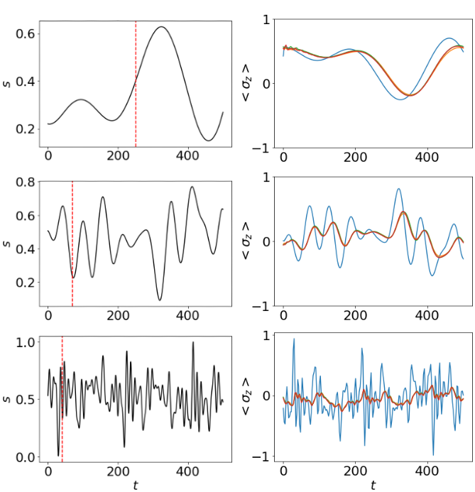
Figure 2: (left) Examples of input sequences at three different frequency scales $f=0.2$ (top), $f=1$ (middle), $f=5$ (bottom). The red vertical dashed line corresponds to the maximum time delay at which the reservoir is successful in remembering past input, based on the results we report later in the manuscript. (right) The corresponding outputs of the reservoir at an interaction strength of $J_{s}=1$, a transverse field of $h=2$,an injection period of $\Delta=2.5$, and a dissipation strength of $\Gamma=0.01$.

II.2 Input and Training

An input signal $s_{k}$ with a frequency scale $f$ is generated as follows. 20 frequencies $\left\{f_{i}\right\}$ are chosen with equal linear spacing in the interval $\left[f/5000,f/50\right]$, thereby producing the series

$$s_{k}=\sum_{i}^{20}\sin\left(2\pi f_{i}t_{k}+2\pi\zeta\right)$$ (5)

where $t_{k}$ is the time after $k$ time steps, and $\zeta$ is a random number uniformly chosen in $\left[0,1\right]$. All input functions are rescaled to have a range between 0 and 1. Examples of such series at different frequency scales $f$ are shown in the left panels of Fig. 2, while the right panels show the corresponding outputs for the dissipative reservoir at a representative choice of parameters.
The input is injected into the systems by means of reinitializing the state of one qubit that we call qubit 1, a widely utilized form of input encoding Mujal et al. [2021]: we trace out the qubit in question and prepare it in a state $|\psi_{s_{k}}\rangle=\sqrt{1-s_{k}}|0\rangle+\sqrt{s_{k}}|1\rangle$, such that

$$\rho\rightarrow|\psi_{s_{k}}\rangle\langle\psi_{s_{k}}|\otimes\text{Tr}_{1}[\rho]$$ (6)

every $\Delta t=L\delta t$, where $L$ is the number of time steps between input injections. We choose $\Delta t$ such that $h\Delta t$ lies in the range prescribed in Ref. Martínez-Peña et al. [2023] for rich linear and non-linear dynamical behaviour.
We employ time multiplexing, where outputs are read at time intervals of $\Delta t/V$, thus allowing for $NV$ virtual nodes. The signals extracted from these nodes, here restricted to $\langle\sigma_{z}\rangle$, are trained in a linear regression to produce the desired function of the input, either a linear memory task $\bar{y}_{k}=s_{k-\tau}$, $\bar{y}_{k}$ being the target, or a non-linear NARMA-n task, which is described and discussed in the Appendix.
The system is trained on multiple sequences and tested using a different sequence, $f$ being the same between the training and testing phases. Tikhonov regularization is employed with a regularization parameter that is allowed to slide to maximize performance. The performance of the reservoir in a memory task with time delay $\tau$, here referred to as the memory capacity, is quantified as

$$C^{\tau}_{STM}=\frac{\text{cov}^{2}(y,\bar{y}^{\tau})}{\sigma_{y}^{2}\sigma_{\bar{y}^{\tau}}^{2}}$$ (7)

where $y$ is the output signal of the reservoir. The memory capacity is subject to the fading memory property of the reservoir computer Dambre et al. [2012]; it must vanish for sufficiently large $\tau$. Thus the total memory capacity of the reservoir may be defined as

$$C_{\text{STM}}=\sum_{\tau=0}^{\infty}C_{\text{STM}}^{\tau}$$ (8)

II.3 Entanglement

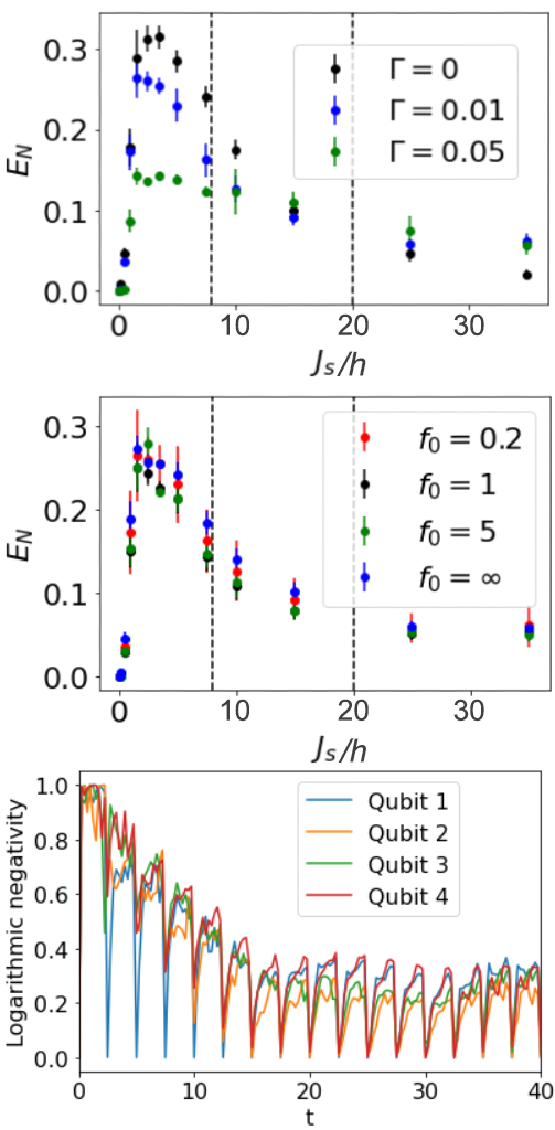
Figure 3: (top) Entanglement vs. interaction strength for the reservoir at a transverse field of $h=2$, and an injection period of $\Delta t=2.5$. The input of frequency of the signal is fixed at $f=0.2$ while the dissipation strength is varied. (middle) Same as top but the dissipation strength is fixed at $\Gamma=0.01$ and the input frequency is varied. The black lines mark the boundary of the dynamical phase transition reported in Martínez-Peña et al. [2021]. (bottom) An example of the logarithmic negativity as a function of time - the entanglement abruptly drops whenever the input is injected. Each color corresponds to the bipartition in which the respective qubit labeled in the legend is isolated.

Quantum entanglement is measured by means of the logarithmic negativity Vidal and Werner [2002], Plenio [2005]

$$E_{N}(\rho)=\log_{2}\|\rho^{\Gamma_{A}}\|_{1}$$ (9)

where $\rho^{\Gamma_{A}}$ is the partial transpose with respect to subsystem A; all bipartitions are averaged over. An example of the behaviour of this quantity is shown in Fig. 3 (top inset), where 4 different bipartitions are shown, each isolating one of the 4 qubits. The entanglement experiences a sudden drop each time the input enters the system, especially the bipartition isolating qubit 1, into which the input is injected.

III Results and Discussion

We commence by presenting the results for the logarithmic negativity measure of entanglement, which we employ to quantify quantumness. Those results are plotted in Fig. 3 against the interaction strength for a variety of dissipation strengths and input of frequencies, at a transverse field of $h=2$, and an injection period of $\Delta t=2.5$. In this figure and all subsequent figures, the critical region between the black lines is that in which the dynamical phase transition takes place in the unitary reservoir between thermalization, to the left of the region, and localization, to the right Martínez-Peña et al. [2021].
A few interesting properties stand out. Firstly, we note that the logarithmic negativity is at its highest to the left of the dynamical phase transition, well into the ergodic regime, where thermalization leads to the spreading of entanglement throughout the system. On the other hand, entanglement is lowest at the extremes: at very high interaction strength the system is deep into the many-body localized phase and the spread of entanglement is stifled, and at very low interaction strength the spins interact too weakly to be entangled. The interaction strength that maximizes entanglement is marked with a red line in all subsequent figures. We also note that the average entanglement goes down as we ramp up the dissipation, albeit with a qualitatively similar shape as a function of interaction strength; it peaks at virtually the same location and dies at the extremes. However, the entanglement appears to be largely insensitive to the frequency of the input signal.
Now, in order to set the stage, we go to the special case of the unitary reservoir at low frequency, of which Fig. 4a presents some intriguing observations. There, the total memory capacity is computed for the linear memory task. The results for the the non-linear NARMA task, qualitatively similar, are presented in Fig. 10 in the appendix. Fig. 4a shows the evolution of the performance as we ramp up the interaction strength $J_{s}$: deep in the ergodic regime (low $J_{s}$) the performance is poor, but improves rapidly as the system approaches the region of the dynamical phase transition indicated by the back lines.
It’s certainly clear from the left panels of Fig. 4 that no entanglement leads to poor performance - but too much entanglement doesn’t seem to be optimal either, for the maximum of entanglement appears to lead to rather a dip in performance. This idea is emphasized in Fig. 4c, in which the memory capacity is plotted this time against entanglement. Performance is undoubtedly enhanced as entanglement rises from zero - consistent with the presence of an entanglement advantage - but plateaus, or almost falls, when the entanglement becomes too great. This suggests that in the case of the unitary reservoir at low frequency, there exists an entanglement advantage with diminishing returns. While an interesting result, it should be noted that the behavior of the unitary reservoir at low frequency is merely a special case to lay the groundwork for examining the more general case of a reservoir with finite dissipation subjected to an input of arbitrary frequency.

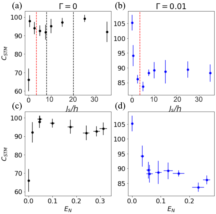
Figure 4: (top) Total memory capacity in the linear memory task vs. interaction strength for the unitary (a) reservoir compared with the dissipative reservoir $\Gamma=0.01$ (b), at a transverse field of $h=2$, an injection period of $\Delta t=2.5$, and the input of frequency of the signal is fixed at $f=0.2$. The black lines mark the boundary of the dynamical phase transition of the unitary reservoir. The red line corresponds to the location of maximum entanglement. (bottom) The same but vs. entanglement.

The behaviour of the non-unitary reservoir is investigated by switching on the dissipation $\Gamma$ in eq. (2). We start at the original conditions of $h=2$, $\Delta t=2.5$, and the low frequency of $f=0.2$. As shown in the top panel of Fig. 3, the ramping of dissipation lowers the entanglement curves. However, the entanglement is clearly insensitive to the input frequency at a given dissipation strength, as is shown in Fig. 3 (bottom). Here, it’s important to remember that the phase boundaries were computed in Ref. Martínez-Peña et al. [2021] for the unitary reservoir.

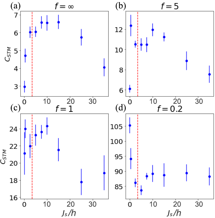
Figure 5: Total memory capacity vs. interaction strength for the dissipative ($\Gamma=0.01$) reservoir at a transverse field of $h=2$, and an injection period of $\Delta t=2.5$, subjected to a variety of input of frequencies $f$, in linear memory tasks at time delay $\tau$. The red line corresponds to the location of maximum entanglement.

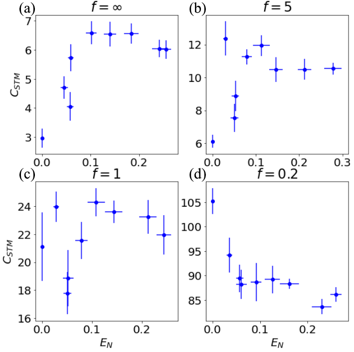
Figure 6: Total memory capacity vs. entanglement for the dissipative ($\Gamma=0.01$) reservoir at a transverse field of $h=2$, and an injection period of $\Delta t=2.5$, subjected to a variety of input of frequencies $f$, in linear memory tasks.

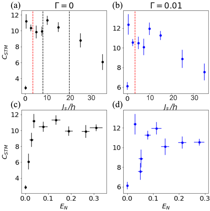
Figure 7: (top) Total memory capacity in the linear memory task vs. interaction strength for the reservoir at a transverse field of $h=2$, and an injection period of $\Delta t=2.5$, subjected to an input frequency of $f=5$, at the dissipation strengths $\Gamma=0$ (a) and $\Gamma=0.01$ (b). The black lines mark the boundary of the dynamical phase transition of the unitary reservoir. The red line corresponds to the location of maximum entanglement. (bottom) The same but vs. entanglement.

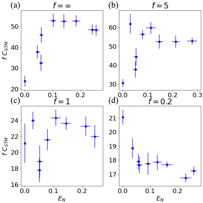
Figure 8: The same as Fig. 6 but with the y-axis of the frequency rescaled by a factor of the input frequency.

The behaviour of the memory capacity in the dissipative reservoir subject to an input frequency of $f=0.2$, as illustrated with an example in Fig. 4b, is rather odd: it develops an abrupt and steep rise at very low interaction strength, where there is little entanglement. Such a jump in behaviour, present in both the linear memory task shown here, and the NARMA task in Fig. 10 in the appendix, makes for a rather striking sight upon comparing the black curves, with zero dissipation, to the blue curves, where even a small amount of dissipation is introduced. It indicates a discontinuity in the dissipative reservoir at low interaction strength and calls into question the presence of the entanglement advantage that is very clear in the case of the unitary reservoir, as illustrated in the bottom right panel of Fig. 4 where the total memory capacity is plotted against the entanglement.
The key to unravelling this quandary lies in generalizing the investigation even further to study the effect of the input frequency. This is accomplished in Fig. 5, which reports the linear memory capacities at the usual conditions of field and injection period, and at a dissipation of $\Gamma=0.01$, but computed for different input frequencies (the corresponding NARMA results are presented in Fig. 11). Here, $f=\infty$ corresponds to a sequence of random floats between 0 and 1 with no continuity. The entanglement advantage is decidedly restored by raising the input frequency, as the performance starts exhibiting a peak at intermediate connectivities.
The return of the entanglement advantage is corroborated by Fig. 6 (whose NARMA counterpart is Fig. 12) , where the total memory capacity as a function of entanglement may be seen to evolve from one extreme to the other. At low frequency, there is a very clear entanglement disadvantage as previously observed, as maximum memory performance occurs where entanglement is smallest and quantum effects are suppressed. As the frequency of the input signal rises, however, the performance enhancement at low entanglement gradually fades. In those high-frequency cases, the entangled systems are significantly better than the non-entangled systems, albeit with diminishing returns on the benefit of entanglement, since performance saturates as entanglement rises. This suggests that there may be an optimal amount of entanglement for memory performance.
One interpretation of this phenomenon is that, while as low a frequency as $0.2$ was perfectly fine for the unitary reservoir, in the presence of a finite amount of dissipation it is so low as to give rise to an incongruence of covariance dimension and performance, as may be seen by comparing Fig. 4 and Fig. 9, and a fading of the entanglement advantage. This reveals that the presence of the entanglement advantage is dependent on the input frequency - however, this scarcely detracts from the significance of the entanglement advantage, as a higher frequency signal is intrinsically more difficult to process. This is consistent with the observation of quantum advantages in highly stochastic and random systems Dale et al. [2015], Blank et al. [2021], Korzekwa and Lostaglio [2021].
The revival of the entanglement advantage in the dissipative reservoir at high frequency raises an important question: how does the unitary reservoir operate at high frequency? Fig. 7 offers an answer to that question by showing the total memory capacities in the linear memory task at $f=5$ (NARMA, once again qualitatively similar, is presented in Fig. 13 in the appendix), comparing the unitary reservoir and the case with a small amount of dissipation ($\Gamma=0.01$). The entanglement advantage is very much present in both cases, as shown in the bottom panels of Fig. 7. Also noteworthy is that the small amount of dissipation seems to result in a small improvement in memory capacity especially at low connectivity (obvious on comparing the leftmost points in the top panels of Fig. 7), which is consistent with the observation reported in Götting et al. [2023], and the ideas presented in Domingo et al. [2023], Suzuki et al. [2022a].
Finally, we recast the data in Fig. 6 in a new light, namely by multiplying the total memory capacities by the input frequency, as shown in Fig. 8. The point of this recasting is to render the comparison of the memory capacities between different frequencies more fair; lower frequency tasks are much easier because they contain fewer temporal features, and so this rescaling gives an estimate of the memory performance with respect to the number of features per unit time. In the case of $f_{\infty}$, which again is merely shorthand for the sequence of random floats, we rescaled the total memory capacity by comparing the frequency of stationary points in that case with the frequency of stationary points at $f=5$. The additional insight revealed Fig. 8 is that as we raise the frequency from $f=0.2$ (where the best performance is by the non-entangled system), the points corresponding to the entangled systems are the ones that rise up to effect the entanglement advantage, rather than the non-entangled system falling off. Indeed, the performance of the unentangled system remains quite consistent throughout the range of input frequencies.

IV Conclusions and Outlook

We studied the performance of a spin network QRC system in linear and non-linear memory tasks, and how it relates to such things as the frequency of the input signal, the presence of dissipation in the system, and quantumness as measured by entanglement.
In the open system, the most general case, it’s clear that the presence of the entanglement advantage is frequency-dependent. Too low a frequency of input signal constitutes too easy a task and the entanglement advantage wanes, and the classical limit with weak interactions and no entanglement performs better in linear and non-linear memory tasks. But in the presence of a sufficiently involved signal that fluctuates rapidly enough, the system appears to derive great benefit from quantum entanglement, and the entanglement advantage manifests itself in both types of tasks. In those high-frequency cases where quantumness is desirable, our results suggest that there may be a particular amount of entanglement that conduces to optimal memory performance.
Possible extensions of this study include the integration of neuromorphic elements into the reservoir. One such possibility involves exploring different reservoir architectures inspired by brain networks, which have been shown to be amenable to being coarse-grained to appropriately large scales while retaining much of their dynamical behavior Kora and Simon [2023]. Another possibility involves studying the potential dependence of the performance of the system on system size, i.e., how it scales with the number of qubits. Furthermore, there is the prospect of investigating spin network reservoirs handling tasks that can learn functions of multiple inputs, in a manner inspired by the brain’s reception of multiple sensory stimuli and processing them in conjunction.
One among several promising avenues is that of quantum computation and simulation with neutral atoms, with which the possibilities are myriad Henriet et al. [2020]; Rydberg atoms are exceptional candidates for the implementation of QRC Bravo et al. [2022] on account of their strong interactions, controllable states, and long coherence times – characteristics that make them ideal for creating highly interactive and adaptable quantum reservoirs. Neutral atoms may be used to implement both the quantum Ising model Scholl et al. [2021], which sits at the foundation of spin-network QRC; and the XY model Barredo et al. [2015], Orioli et al. [2018], which would be a fascinating platform on which to implement an additional level of complexity and non-linearity in a quantum reservoir. This is one among several platforms that are well-suited for QRC implementation, such as superconducting qubits Suzuki et al. [2022a], photonics García-Beni et al. [2023], and trapped ions Häffner et al. [2008]. Making contact with such implementations will be the topic of future investigation.

V Acknowledgments

This work was supported by the National Research Council through its Applied Quantum Computing Challenge Program, the Natural Sciences and Engineering Research Council (NSERC) of Canada through its NSERC Discovery Grant Program, the Alberta Major Innovation Fund, and Quantum City. We would also like to thank Aaron Goldberg for the useful discussions and feedback.

VI Appendix

VI.1 Principal Component Analysis

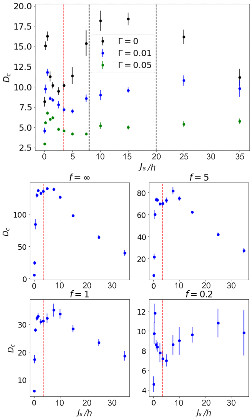
Figure 9: Covariance dimension vs. interaction strength at the same sets of conditions as Fig. 3. The black lines mark the boundary of the dynamical phase transition reported in Martínez-Peña et al. [2021]. The red line corresponds to the location of maximum entanglement.

To estimate the dimensionality of the manifold to which the dynamics is restricted, principal component analysis is performed as in Götting et al. [2023]. Let the quantum dynamics of the system be represented by the trajectory of the vector evolution $\bf X=(x_{0},x_{1},\ldots)$, where $\bf x_{i}$ are the density matrices of the system sampled at the multiplexed intervals $\Delta t/V$. A random time index is chosen and a cluster of $d+1$ nearest neighbours is determined and combined into a matrix $X_{i0}$, of which the covariance matrix is computed

$$C_{\bf{X}_{i_{0}}}=\frac{1}{N_{d}-1}(\bf{X}_{i_{0}}-\bar{\bf{X}}_{i_{0}})(\bf{X}_{i_{0}}-\bar{\bf{X}}_{i_{0}})^{T}$$ (10)

The covariance dimension is the number of principal components of $C_{X_{i_{0}}}$ greater than $\epsilon=10^{-6}$ (which is fixed at a small value for all points), and is averaged over many iterations Götting et al. [2023].

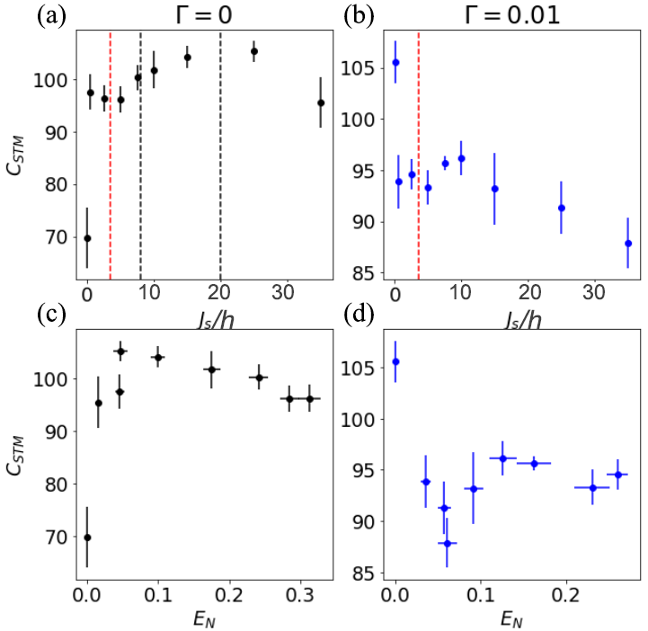
Figure 10: Same as Fig. 4 but for the NARMA task.

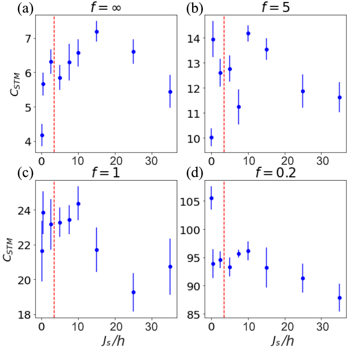
Figure 11: Same as Fig. 5 but for the NARMA task.

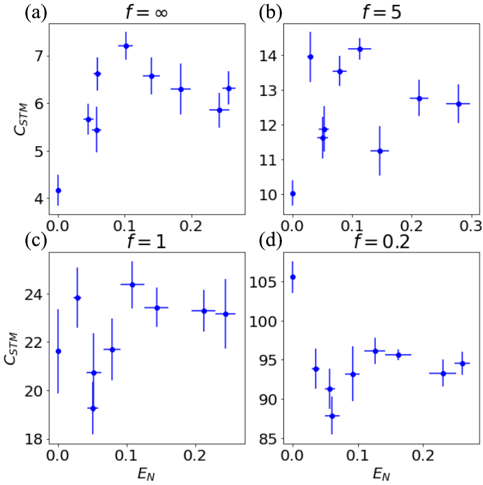
Figure 12: Same as Fig. 5 but for the NARMA task.

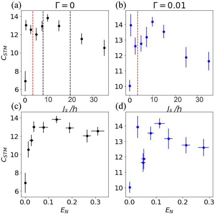
Figure 13: Same as Fig. 7 but for the NARMA tasks

The relevant PCA results are summarized in Fig. 9. The bottom panels ($f=0.2$) makes it clear that the small dip in performance observed in Fig. 4 is rather amplified, as the dimensionality experiences a much more pronounced dip at that region. There is also a substantial boost in the dimensionality of the unitary reservoir conferred by criticality, which is consistent with the performance boost at the dynamical phase transition observed in Martínez-Peña et al. [2021]. As dissipation is raised, covariance dimension is suppressed.
The top panel of Fig. 9 highlights the strangeness of the ”anomaly” in Fig. 4; upon comparing the two figures, it’s clear that there is a congrience between covariance dimension and memory performance of the unitary reservoir, as they both rise from zero, peak, experience a dip, peak again near criticality, and then fall again. When dissipation is switched on, one can see the anomaly in Fig. 4, where performance blows up at low interaction strength all of a sudden, which is not followed by a corresponding rise in dimensionality in the top panel of Fig. 9.
The congruence of performance and dimensionality in the dissipative reservoir is re-established at sufficiently high frequency, when the entanglement advantage is restored. This may be seen by comparing Fig. 9 and Fig 5. The dimensionality curves, consistently familiar in shape, are only qualitatively resembled by the memory capacity curves at sufficiently high frequency. In short, our results indicate that the congruence between performance and dimensionality goes hand-in-hand with the presence of the entanglement advantage.

VI.2 The Non-Linear NARMA Task

The NARMA-n task Atiya and Parlos [2000] is given by

$$\bar{y}_{k+1}=\alpha\bar{y}_{k}+\beta\bar{y}_{k}\left(\sum_{j=1}^{n}\bar{y}_{k-j}\right)+\gamma s_{k-n}s_{k-1}+\delta,$$ (11)

where $n$ is the maximum time delay and $\alpha=0.3$, $\beta=0.002$, $\gamma=1.5$, $\delta=0.1$, convergent at a great range of frequencies. Figs. 10, 11, 12, 13 present the NARMA counterparts of the results of the main text, which are qualitatively similar in nature.

References

- Abreu Araujo et al. [2020] F. Abreu Araujo, M. Riou, J. Torrejon, S. Tsunegi, D. Querlioz, K. Yakushiji, A. Fukushima, H. Kubota, S. Yuasa, M. D. Stiles, and J. Grollier. Role of non-linear data processing on speech recognition task in the framework of reservoir computing. Scientific Reports, 10(1), Jan. 2020. ISSN 2045-2322. doi: 10.1038/s41598-019-56991-x. URL http://dx.doi.org/10.1038/s41598-019-56991-x.
- Antonik et al. [2017] P. Antonik, M. Haelterman, and S. Massar. Brain-inspired photonic signal processor for generating periodic patterns and emulating chaotic systems. Physical Review Applied, 7(5), May 2017. ISSN 2331-7019. doi: 10.1103/physrevapplied.7.054014. URL http://dx.doi.org/10.1103/PhysRevApplied.7.054014.
- Atiya and Parlos [2000] A. Atiya and A. Parlos. New results on recurrent network training: unifying the algorithms and accelerating convergence. IEEE Transactions on Neural Networks, 11(3):697–709, 2000. doi: 10.1109/72.846741.
- Ballarin et al. [2023] G. Ballarin, P. Dellaportas, L. Grigoryeva, M. Hirt, S. van Huellen, and J.-P. Ortega. Reservoir computing for macroeconomic forecasting with mixed-frequency data. International Journal of Forecasting, Dec. 2023. ISSN 0169-2070. doi: 10.1016/j.ijforecast.2023.10.009. URL http://dx.doi.org/10.1016/j.ijforecast.2023.10.009.
- Banchi [2023] L. Banchi. Accuracy vs memory advantage in the quantum simulation of stochastic processes, 2023. URL https://arxiv.org/abs/2312.13473.
- Barredo et al. [2015] D. Barredo, H. Labuhn, S. Ravets, T. Lahaye, A. Browaeys, and C. S. Adams. Coherent excitation transfer in a spin chain of three rydberg atoms. Phys. Rev. Lett., 114:113002, Mar 2015. doi: 10.1103/PhysRevLett.114.113002. URL https://link.aps.org/doi/10.1103/PhysRevLett.114.113002.
- Blank et al. [2021] C. Blank, D. K. Park, and F. Petruccione. Quantum-enhanced analysis of discrete stochastic processes. npj Quantum Information, 7(1), Aug. 2021. ISSN 2056-6387. doi: 10.1038/s41534-021-00459-2. URL http://dx.doi.org/10.1038/s41534-021-00459-2.
- Bravo et al. [2022] R. A. Bravo, K. Najafi, X. Gao, and S. F. Yelin. Quantum reservoir computing using arrays of rydberg atoms. PRX Quantum, 3:030325, Aug 2022. doi: 10.1103/PRXQuantum.3.030325. URL https://link.aps.org/doi/10.1103/PRXQuantum.3.030325.
- Breuer and Petruccione [2002] H. Breuer and F. Petruccione. The Theory of Open Quantum Systems. Oxford University Press, Oxford, 2002.
- Dale et al. [2015] H. Dale, D. Jennings, and T. Rudolph. Provable quantum advantage in randomness processing. Nature Communications, 6(1), Sept. 2015. ISSN 2041-1723. doi: 10.1038/ncomms9203. URL http://dx.doi.org/10.1038/ncomms9203.
- Dambre et al. [2012] J. Dambre, D. Verstraeten, B. Schrauwen, and S. Massar. Information processing capacity of dynamical systems. Scientific Reports, 2:514, 2012. doi: 10.1038/srep00514. URL https://doi.org/10.1038/srep00514.
- Dion et al. [2018] G. Dion, S. Mejaouri, and J. Sylvestre. Reservoir computing with a single delay-coupled non-linear mechanical oscillator. Journal of Applied Physics, 124(15), Oct. 2018. ISSN 1089-7550. doi: 10.1063/1.5038038. URL http://dx.doi.org/10.1063/1.5038038.
- Domingo et al. [2023] L. Domingo, G. Carlo, and F. Borondo. Taking advantage of noise in quantum reservoir computing. Scientific Reports, 13(1), May 2023. ISSN 2045-2322. doi: 10.1038/s41598-023-35461-5. URL http://dx.doi.org/10.1038/s41598-023-35461-5.
- Dudas et al. [2023] J. Dudas, B. Carles, E. Plouet, F. A. Mizrahi, J. Grollier, and D. Marković. Quantum reservoir computing implementation on coherently coupled quantum oscillators. npj Quantum Information, 9(1), July 2023. ISSN 2056-6387. doi: 10.1038/s41534-023-00734-4. URL http://dx.doi.org/10.1038/s41534-023-00734-4.
- Eliasmith et al. [2012] C. Eliasmith, T. C. Stewart, X. Choo, T. Bekolay, T. DeWolf, Y. Tang, and D. Rasmussen. A large-scale model of the functioning brain. Science, 338(6111):1202–1205, Nov. 2012. ISSN 1095-9203. doi: 10.1126/science.1225266. URL http://dx.doi.org/10.1126/science.1225266.
- Fry et al. [2023] D. Fry, A. Deshmukh, S. Y.-C. Chen, V. Rastunkov, and V. Markov. Optimizing quantum noise-induced reservoir computing for nonlinear and chaotic time series prediction. Scientific Reports, 13(1), Nov. 2023. ISSN 2045-2322. doi: 10.1038/s41598-023-45015-4. URL http://dx.doi.org/10.1038/s41598-023-45015-4.
- Fujii and Nakajima [2017] K. Fujii and K. Nakajima. Harnessing disordered-ensemble quantum dynamics for machine learning. Phys. Rev. Appl., 8:024030, Aug 2017. doi: 10.1103/PhysRevApplied.8.024030. URL https://link.aps.org/doi/10.1103/PhysRevApplied.8.024030.
- Fujii and Nakajima [2021] K. Fujii and K. Nakajima. Quantum reservoir computing: A reservoir approach toward quantum machine learning on near-term quantum devices. In K. Nakajima and I. Fischer, editors, Reservoir Computing, Natural Computing Series. Springer, Singapore, 2021. doi: 10.1007/978-981-13-1687-6˙18. URL https://doi.org/10.1007/978-981-13-1687-6_18.
- Furuta et al. [2018] T. Furuta, K. Fujii, K. Nakajima, S. Tsunegi, H. Kubota, Y. Suzuki, and S. Miwa. Macromagnetic simulation for reservoir computing utilizing spin dynamics in magnetic tunnel junctions. Physical Review Applied, 10(3), Sept. 2018. ISSN 2331-7019. doi: 10.1103/physrevapplied.10.034063. URL http://dx.doi.org/10.1103/PhysRevApplied.10.034063.
- García-Beni et al. [2023] J. García-Beni, G. L. Giorgi, M. C. Soriano, and R. Zambrini. Scalable photonic platform for real-time quantum reservoir computing. Physical Review Applied, 20(1), July 2023. ISSN 2331-7019. doi: 10.1103/physrevapplied.20.014051. URL http://dx.doi.org/10.1103/PhysRevApplied.20.014051.
- Gartside et al. [2022] J. C. Gartside, K. D. Stenning, A. Vanstone, H. H. Holder, D. M. Arroo, T. Dion, F. Caravelli, H. Kurebayashi, and W. R. Branford. Reconfigurable training and reservoir computing in an artificial spin-vortex ice via spin-wave fingerprinting. Nature Nanotechnology, 17(5):460–469, May 2022. ISSN 1748-3395. doi: 10.1038/s41565-022-01091-7. URL http://dx.doi.org/10.1038/s41565-022-01091-7.
- Gilboa and McClean [2023] D. Gilboa and J. R. McClean. Exponential quantum communication advantage in distributed learning, 2023.
- Götting et al. [2023] N. Götting, F. Lohof, and C. Gies. Exploring quantumness in quantum reservoir computing. Phys. Rev. A, 108:052427, Nov 2023. doi: 10.1103/PhysRevA.108.052427. URL https://link.aps.org/doi/10.1103/PhysRevA.108.052427.
- Govia et al. [2021] L. C. G. Govia, G. J. Ribeill, G. E. Rowlands, H. K. Krovi, and T. A. Ohki. Quantum reservoir computing with a single nonlinear oscillator. Physical Review Research, 3(1), Jan. 2021. ISSN 2643-1564. doi: 10.1103/physrevresearch.3.013077. URL http://dx.doi.org/10.1103/PhysRevResearch.3.013077.
- Häffner et al. [2008] H. Häffner, C. Roos, and R. Blatt. Quantum computing with trapped ions. Physics Reports, 469(4):155–203, 2008. ISSN 0370-1573. doi: https://doi.org/10.1016/j.physrep.2008.09.003. URL https://www.sciencedirect.com/science/article/pii/S0370157308003463.
- Henriet et al. [2020] L. Henriet, L. Beguin, A. Signoles, T. Lahaye, A. Browaeys, G.-O. Reymond, and C. Jurczak. Quantum computing with neutral atoms. Quantum, 4:327, 2020. doi: 10.22331/q-2020-09-21-327. URL https://doi.org/10.22331/q-2020-09-21-327.
- Jaeger and Haas [2004] H. Jaeger and H. Haas. Harnessing nonlinearity: Predicting chaotic systems and saving energy in wireless communication. Science, 304:78–80, 2004. doi: 10.1126/science.1091277. URL https://www.science.org/doi/10.1126/science.1091277.
- Kora and Simon [2023] Y. Kora and C. Simon. Coarse-graining and criticality in the human connectome, 2023.
- Korzekwa and Lostaglio [2021] K. Korzekwa and M. Lostaglio. Quantum advantage in simulating stochastic processes. Physical Review X, 11(2), Apr. 2021. ISSN 2160-3308. doi: 10.1103/physrevx.11.021019. URL http://dx.doi.org/10.1103/PhysRevX.11.021019.
- Körber et al. [2023] L. Körber, C. Heins, T. Hula, J.-V. Kim, S. Thlang, H. Schultheiss, J. Fassbender, and K. Schultheiss. Pattern recognition in reciprocal space with a magnon-scattering reservoir. Nature Communications, 14(1), July 2023. ISSN 2041-1723. doi: 10.1038/s41467-023-39452-y. URL http://dx.doi.org/10.1038/s41467-023-39452-y.
- Larger et al. [2017] L. Larger, A. Baylón-Fuentes, R. Martinenghi, V. S. Udaltsov, Y. K. Chembo, and M. Jacquot. High-speed photonic reservoir computing using a time-delay-based architecture: Million words per second classification. Physical Review X, 7(1), Feb. 2017. ISSN 2160-3308. doi: 10.1103/physrevx.7.011015. URL http://dx.doi.org/10.1103/PhysRevX.7.011015.
- Luchnikov et al. [2019] I. A. Luchnikov, S. V. Vintskevich, H. Ouerdane, and S. N. Filippov. Simulation complexity of open quantum dynamics: Connection with tensor networks. Physical Review Letters, 122(16), Apr. 2019. ISSN 1079-7114. doi: 10.1103/physrevlett.122.160401. URL http://dx.doi.org/10.1103/PhysRevLett.122.160401.
- Maass et al. [2002] W. Maass, T. Natschläger, and H. Markram. Real-time computing without stable states: A new framework for neural computation based on perturbations. Neural Computation, 14(11):2531–2560, 2002. doi: 10.1162/089976602760407955. URL https://doi.org/10.1162/089976602760407955.
- Martínez-Peña et al. [2021] R. Martínez-Peña, G. L. Giorgi, J. Nokkala, M. C. Soriano, and R. Zambrini. Dynamical phase transitions in quantum reservoir computing. Phys. Rev. Lett., 127:100502, Aug 2021. doi: 10.1103/PhysRevLett.127.100502. URL https://link.aps.org/doi/10.1103/PhysRevLett.127.100502.
- Martínez-Peña et al. [2023] R. Martínez-Peña, J. Nokkala, G. L. Giorgi, R. Zambrini, and M. C. Soriano. Information processing capacity of spin-based quantum reservoir computing systems. Cognitive Computation, 15:1440–1451, 2023. doi: 10.1007/s12559-020-09772-y. URL https://link.springer.com/article/10.1007/s12559-020-09772-y.
- Martínez-Peña et al. [2020] R. Martínez-Peña, J. Nokkala, G. L. Giorgi, R. Zambrini, and M. C. Soriano. Information processing capacity of spin-based quantum reservoir computing systems. Cognitive Computation, 15(5):1440–1451, Oct. 2020. ISSN 1866-9964. doi: 10.1007/s12559-020-09772-y. URL http://dx.doi.org/10.1007/s12559-020-09772-y.
- Meffan et al. [2023] C. Meffan, T. Ijima, A. Banerjee, J. Hirotani, and T. Tsuchiya. Non-linear processing with a surface acoustic wave reservoir computer. Microsystem Technologies, 29(8):1197–1206, May 2023. ISSN 1432-1858. doi: 10.1007/s00542-023-05463-4. URL http://dx.doi.org/10.1007/s00542-023-05463-4.
- Motamedi et al. [2023] A. Motamedi, H. Zadeh-Haghighi, and C. Simon. Correlations between quantumness and learning performance in reservoir computing with a single oscillator, 2023. URL https://arxiv.org/abs/2304.03462.
- Mujal et al. [2021] P. Mujal, J. Nokkala, R. Martínez-Peña, G. L. Giorgi, M. C. Soriano, and R. Zambrini. Analytical evidence of nonlinearity in qubits and continuous-variable quantum reservoir computing. J. of Phys. Complex., 2(4):045008, 2021. doi: 10.1088/2632-072X/ac340e.
- Nakajima et al. [2019] K. Nakajima, K. Fujii, M. Negoro, K. Mitarai, and M. Kitagawa. Boosting computational power through spatial multiplexing in quantum reservoir computing. Physical Review Applied, 11(3):034021–1, Mar. 2019. doi: 10.1103/physrevapplied.11.034021. URL https://doi.org/10.1103/physrevapplied.11.034021.
- Nicola and Clopath [2017] W. Nicola and C. Clopath. Supervised learning in spiking neural networks with force training. Nature Communications, 8(1), Dec. 2017. ISSN 2041-1723. doi: 10.1038/s41467-017-01827-3. URL http://dx.doi.org/10.1038/s41467-017-01827-3.
- Nokkala et al. [2021] J. Nokkala, R. Martínez-Peña, G. L. Giorgi, V. Parigi, M. C. Soriano, and R. Zambrini. Gaussian states of continuous-variable quantum systems provide universal and versatile reservoir computing. Communications Physics, 4(1), Mar. 2021. ISSN 2399-3650. doi: 10.1038/s42005-021-00556-w. URL http://dx.doi.org/10.1038/s42005-021-00556-w.
- Orioli et al. [2018] A. P. n. Orioli, A. Signoles, H. Wildhagen, G. Günter, J. Berges, S. Whitlock, and M. Weidemüller. Relaxation of an isolated dipolar-interacting rydberg quantum spin system. Phys. Rev. Lett., 120:063601, Feb 2018. doi: 10.1103/PhysRevLett.120.063601. URL https://link.aps.org/doi/10.1103/PhysRevLett.120.063601.
- Palsson et al. [2017] M. S. Palsson, M. Gu, J. Ho, H. M. Wiseman, and G. J. Pryde. Experimentally modeling stochastic processes with less memory by the use of a quantum processor. Science Advances, 3(2), Feb. 2017. ISSN 2375-2548. doi: 10.1126/sciadv.1601302. URL http://dx.doi.org/10.1126/sciadv.1601302.
- Papp et al. [2021] A. Papp, W. Porod, and G. Csaba. Nanoscale neural network using non-linear spin-wave interference. Nature Communications, 12(1), Nov. 2021. ISSN 2041-1723. doi: 10.1038/s41467-021-26711-z. URL http://dx.doi.org/10.1038/s41467-021-26711-z.
- Pfeuty and Elliott [1971] P. Pfeuty and R. J. Elliott. The ising model with a transverse field. ii. ground state properties. Journal of Physics C: Solid State Physics, 4:2370, 1971.
- Plenio [2005] M. B. Plenio. Logarithmic negativity: A full entanglement monotone that is not convex. Phys. Rev. Lett., 95:090503, Aug 2005. doi: 10.1103/PhysRevLett.95.090503. URL https://link.aps.org/doi/10.1103/PhysRevLett.95.090503.
- Scholl et al. [2021] P. Scholl, M. Schuler, H. Williams, et al. Quantum simulation of 2d antiferromagnets with hundreds of rydberg atoms. Nature, 595:233–238, 2021. doi: 10.1038/s41586-021-03585-1. URL https://doi.org/10.1038/s41586-021-03585-1.
- Stewart et al. [2012] T. C. Stewart, T. Bekolay, and C. Eliasmith. Learning to select actions with spiking neurons in the basal ganglia. Frontiers in Neuroscience, 6, 2012. ISSN 1662-4548. doi: 10.3389/fnins.2012.00002. URL http://dx.doi.org/10.3389/fnins.2012.00002.
- Stieg et al. [2011] A. Z. Stieg, A. V. Avizienis, H. O. Sillin, C. Martin‐Olmos, M. Aono, and J. K. Gimzewski. Emergent criticality in complex turing b‐type atomic switch networks. Advanced Materials, 24(2):286–293, Oct. 2011. ISSN 1521-4095. doi: 10.1002/adma.201103053. URL http://dx.doi.org/10.1002/adma.201103053.
- Stinchcombe [1973] R. B. Stinchcombe. Ising model in a transverse field. i. basic theory. Journal of Physics C: Solid State Physics, 6(15):2459, 1973.
- Sunada and Uchida [2021] S. Sunada and A. Uchida. Photonic neural field on a silicon chip: large-scale, high-speed neuro-inspired computing and sensing. Optica, 8(11):1388, Nov. 2021. ISSN 2334-2536. doi: 10.1364/optica.434918. URL http://dx.doi.org/10.1364/OPTICA.434918.
- Suzuki et al. [2022a] Y. Suzuki, Q. Gao, K. Pradel, et al. Natural quantum reservoir computing for temporal information processing. Scientific Reports, 12:1353, 2022a. doi: 10.1038/s41598-022-05061-w. URL https://doi.org/10.1038/s41598-022-05061-w.
- Suzuki et al. [2022b] Y. Suzuki, Q. Gao, K. C. Pradel, K. Yasuoka, and N. Yamamoto. Natural quantum reservoir computing for temporal information processing. Scientific Reports, 12(1), Jan. 2022b. ISSN 2045-2322. doi: 10.1038/s41598-022-05061-w. URL http://dx.doi.org/10.1038/s41598-022-05061-w.
- Tanaka et al. [2019] G. Tanaka, T. Yamane, J. B. Héroux, R. Nakane, N. Kanazawa, S. Takeda, H. Numata, D. Nakano, and A. Hirose. Recent advances in physical reservoir computing: A review. Neural Networks, 115:100–123, July 2019. ISSN 0893-6080. doi: 10.1016/j.neunet.2019.03.005. URL http://dx.doi.org/10.1016/j.neunet.2019.03.005.
- Torrejon et al. [2017] J. Torrejon, M. Riou, F. A. Araujo, S. Tsunegi, G. Khalsa, D. Querlioz, P. Bortolotti, V. Cros, K. Yakushiji, A. Fukushima, H. Kubota, S. Yuasa, M. D. Stiles, and J. Grollier. Neuromorphic computing with nanoscale spintronic oscillators. Nature, 547(7664):428–431, July 2017. ISSN 1476-4687. doi: 10.1038/nature23011. URL http://dx.doi.org/10.1038/nature23011.
- Tsunegi et al. [2018] S. Tsunegi, T. Taniguchi, S. Miwa, K. Nakajima, K. Yakushiji, A. Fukushima, S. Yuasa, and H. Kubota. Evaluation of memory capacity of spin torque oscillator for recurrent neural networks. Japanese Journal of Applied Physics, 57(12):120307, Oct. 2018. ISSN 1347-4065. doi: 10.7567/jjap.57.120307. URL http://dx.doi.org/10.7567/JJAP.57.120307.
- Vandoorne et al. [2014] K. Vandoorne, P. Mechet, T. Van Vaerenbergh, M. Fiers, G. Morthier, D. Verstraeten, B. Schrauwen, J. Dambre, and P. Bienstman. Experimental demonstration of reservoir computing on a silicon photonics chip. Nature Communications, 5(1), Mar. 2014. ISSN 2041-1723. doi: 10.1038/ncomms4541. URL http://dx.doi.org/10.1038/ncomms4541.
- Verstraeten et al. [2007] D. Verstraeten, B. Schrauwen, M. D’Haene, and D. Stroobandt. An experimental unification of reservoir computing methods. Neural Networks, 20:391–403, 2007. ISSN 0893-6080. doi: 10.1016/j.neunet.2007.04.003. URL https://www.sciencedirect.com/science/article/pii/S089360800700038X.
- Vidal and Werner [2002] G. Vidal and R. F. Werner. Computable measure of entanglement. Phys. Rev. A, 65:032314, Feb 2002. doi: 10.1103/PhysRevA.65.032314. URL https://link.aps.org/doi/10.1103/PhysRevA.65.032314.
- von Neumann [1993] J. von Neumann. First draft of a report on the edvac. IEEE Annals of the History of Computing, 15(4):27–75, 1993. ISSN 1058-6180. doi: 10.1109/85.238389. URL http://dx.doi.org/10.1109/85.238389.
- Yaremkevich et al. [2023] D. D. Yaremkevich, A. V. Scherbakov, L. De Clerk, S. M. Kukhtaruk, A. Nadzeyka, R. Campion, A. W. Rushforth, S. Savel’ev, A. G. Balanov, and M. Bayer. On-chip phonon-magnon reservoir for neuromorphic computing. Nature Communications, 14(1), Dec. 2023. ISSN 2041-1723. doi: 10.1038/s41467-023-43891-y. URL http://dx.doi.org/10.1038/s41467-023-43891-y.