A Constrained Tracking Controller for Ramp and Sinusoidal Reference Signals using Robust Positive Invariance

Abstract

This paper proposes an output feedback controller capable of ensuring steady-state offset-free tracking for ramp and sinusoidal reference signals while ensuring local stability and state and input constraints fulfillment. The proposed solution is derived by jointly exploiting the internal model principle, polyhedral robust positively invariant arguments, and the Extended Farkas’ Lemma. In particular, by considering a generic class of output feedback controller equipped with a feedforward term, a proportional effect, and a double integrator, we offline design the controller’s gains by means of a single bilinear optimization problem. A peculiar feature of the proposed design is that the sets of all the admissible reference signals and the plant’s initial conditions are also offline determined. Simulation results are provided to testify to the effectiveness of the proposed tracking controller and its capability to deal with both state and input constraints.

I Introduction

The set invariance theory is widely used in control, particularly when dealing with constrained systems and stability analysis. Sets are the most appropriate language to specify several system performances, such as determining the domain of attraction or measuring the effect of persistent noise in a feedback loop. One of the most popular approaches in this field is the Lyapunov theory and positive invariance. A positively invariant set is a subset of the state space of a dynamical system with the property that, if the system state is in this set at some time, then it will stay in this set in the future [1, 2].

The Internal Model Principle (IMP) [3] is an essential result for reference tracking problems. IMP provides the conditions under which a stabilizing controller also ensures tracking by assuming an unconstrained feedback control system. As a result, several constrained and unconstrained tracking controllers have been established in the literature from different perspectives. Present techniques vary from Proportional-Integral (PI) controllers to Model Predictive Control (MPC) [4], as well as Reference and Command Governor solutions [5, 6, 7, 8].

In particular, different PI-like control design methods have been developed for a variety of constrained systems that consider algorithms based on Linear Matrix Inequalities (LMIs). The controller developed in [9] deals with linear time-invariant systems, the solution in [10] addresses Linear Parameter-Varying (LPV) systems, and the approach described in [11] is designed for nonlinear systems represented by Takagi-Sugeno (TS) models. Also, linear systems with saturating actuators and additive disturbances using either Riccati equations (ARE) or LMIs are investigated in [12], and uncertain linear systems under control saturation using a “quasi”-LMI approach for periodic references have been considered in [13]. However, these solutions deal only with symmetrical input saturation constraints and define contractive ellipsoidal (or composite ellipsoidal) invariant areas. On the other hand, the PI-like controller with feedforward term proposed in [14] leverages algebraic robust positive invariance relations to define a bilinear optimization design problem capable of simultaneously computing the controller’s parameters and the set of admissible step reference signals. The proposed design methodology guarantees steady-state offset-free tracking, and it can deal with continuous-time linear systems subject to asymmetrical and polyhedral state and input constraints. The discrete-time counterpart of the solution in [14] is presented in [15].

I-A Paper’s contribution

In this manuscript, we extend the solution in [14] (capable of dealing only with step reference signals) to design a controller that addresses a broader class of reference signals, including ramps and sinusoidal signals. The proposed controller’s design procedure can deal with asymmetric and polyhedral state and input constraints. Differently from [14], we consider a generic second-order homogeneous representation of the exogenous reference signal and an enhanced PI-like controller structure with a double integrator term. Such a structure is then leveraged to define the augmented constrained dynamics of the controlled closed-loop system and design the controller using a single bilinear optimization program. The proposed solution has the peculiar feature of allowing the simultaneous design and optimization of the controller’s parameters, controller’s domain of attraction and set of admissible reference signals.

The rest of the paper is organized as follows. Section II proposes the constrained PI-like controller’s design. Section III presents the proposed solution, and Section IV shows a numerical example for ramp and sinusoidal reference signals. Finally, Section V concludes the paper.

II Constrained Control Problem

Consider a Linear Time-Invariant Continuous-Time (LTIC) system in the form

$$\begin{array}[]{rcl}\dot{x}(t)&=&Ax(t)+Bu(t),\\ y(t)&=&Cx(t),\end{array}$$ (1)

where $x(t)\in\mathbb{R}^{n}$ is the state vector, $u(t)\in\mathbb{R}^{m}$ the control input vector, and $y(t)\in\mathbb{R}$ the measurement vector. The system matrices $(A,B,C)$ are of suitable dimensions, with $(A,B)$ controllable and $(C,A)$ observable.

Remark 1

For reference tracking purposes, in (1) we have assumed that the output of the system is scalar (i.e., $y(t)\in\mathbb{R}$). It is worth remarking that such a choice is not dictated by any intrinsic limitation of the solution hereafter proposed, but it is made only for the sake of clarity and to improve as much as possible the description and readability of the proposed solution.

Definition 1

A polyhedral set $\mathcal{P}(\phi)\subseteq\mathbb{R}^{n}$ is said to be Robust Positively Invariant (RPI) for the system $\dot{x}(t)=f(x(t),d(t)),$ $t\geq 0,$ $x(t)\in\mathbb{R}^{n},$ $d(t)\in\Delta(\psi)\subseteq\mathbb{R}^{n_{d}}$, where $\Delta(\psi)$ is a compact polyhedral set, if for any initial state $x(0)\in\mathcal{P}(\phi),$ the state trajectory $x(t)$ remains bounded inside $\mathcal{P}(\phi),\forall\,t\geq 0$ and $\forall\,d(t)\in\Delta(\psi).$

The state and input vectors are assumed to be subject to the following state and input constraints

$$x(t)\in\mathcal{X}=\{x(t):Xx(t)\leq\textbf{1${}_{l_{x}}$}\},~{}X\in\mathbb{R}^{l_{x}\times n},$$ (2)

$$u(t)\in\mathcal{U}=\{u(t):Uu(t)\leq\textbf{1${}_{l_{u}}$}\},~{}U\in\mathbb{R}^{l_{u}\times m}.$$ (3)

For tracking purposes, we assume that $y(t)$ must track a reference signal given by the homogeneous equation

$$\ddot{r}(t)+\alpha r(t)=0,$$ (4)

where the initial conditions are unknown and $r(t)$ describes

• a ramp signal, i.e., $r(t)=at,~{}t\geq 0,$ if $\alpha=0$,

• a sinusoidal signal $r(t)=a\sin\omega t,~{}t\geq 0,$ if $\alpha=\omega^{2}$.

Also, the reference signal $r(t)$ is bounded in an asymmetric hyperrectangle described by the set

$$\mathcal{R}(\rho)=\{r(t):Rr(t)\leq\rho\},$$ (5)

where $R=\begin{bmatrix}~{}~{}I\\ -I\end{bmatrix}\in\mathbb{R}^{2\times 2}$ and $\rho=\begin{bmatrix}\rho_{1}\\ \rho_{2}\end{bmatrix}\in\mathbb{R}^{2}$.

Furthermore, the bounds of the ramp reference signal can be interpreted, for a given time $t$, as the slope $a=\dfrac{\rho}{t}$. For the sinusoidal signal, the bounds of $\mathcal{R}(\rho)$ represent the amplitude $a=\rho$, although the angular frequency $\omega$ takes its place by appearing in the internal model’s reference, which has to be part of the controller’s structure. An additional condition that has to be assumed is $rank\begin{bmatrix}A-\sigma I_{n}&B\\ C&0\end{bmatrix}=n+1$ for $\sigma$ a complex value, such that $\sigma^{2}+\alpha=0$, i.e., the system is free from transmission zeros at the origin for $\alpha=0$ (ramp), or transmission zeros at $\pm j\omega$ for $\alpha=\omega^{2}$ (sinusoidal).

We assume that the tracking controller presents the following structure

$$u(t)=Ky(t)+K_{I_{1}}x_{I_{1}}(t)+K_{I_{2}}x_{I_{2}}(t)+K_{r}r(t),$$ (6)

where $K,K_{I_{1}},K_{I_{2}},K_{r}\in\mathbb{R}^{m}$, $e(t)=r(t)-y(t)$,

$$x_{I_{1}}(t)=\int_{0}^{t}(e(\tau)-\alpha x_{I_{2}})d\tau\in\mathbb{R},$$

$$x_{I_{2}}(t)=\int_{0}^{t}x_{I_{1}}(s)ds\in\mathbb{R},$$

and $\alpha=0$ for a ramp reference signal, $\alpha=\omega^{2}$ for a sinusoidal reference signal.

Remark 2

Note that $Ky$, $K_{I_{1}}x_{I_{1}}$ and $K_{I_{2}}x_{I_{2}}$ define a Proportional and double Integral effect, respectively, while $K_{r}$ is a feedforward term used to improve the reference response, see [16, Chapter 5]. Consequently, according to the IMP [3, Section 9.2.2], any stabilizing controller having the structure of (6), guarantees asymptotic reference tracking. However, since the considered system is subject to state and input constraints, the validity of such a result may be restricted to a bounded state space region where the constraints are inactive.

Problem 1

Consider the constrained plant’s model (1)-(3), the reference constraint (5) and the controller’s structure (6). Design the control gains $(K,K_{I_{1}},K_{I_{2}},K_{r})$ in (6), the vector $\rho$ in (5), and a RPI set $\mathcal{L}\subset\mathbb{R}^{n+2}$, such that for any initial condition $x_{cl}(0)=[x^{T}(0)~{}x^{T}_{I_{1}}(0)~{}x^{T}_{I_{2}}(0)]^{T}\in\mathcal{L},$ the reference $r(t)$ is asymptotically tracked and the constraints (2)-(3) are fulfilled.

A particular case of the previous problem considering piecewise set-point tracking references was investigated in [14]. There, the control law (6) was considered only with one integrator, that is, they do not have the gain $K_{I_{2}}$ and the integral state $x_{I_{2}}$. Then, the closed-loop system is the second-order instead of the third-order as in (7).

III Proposed Solution

Using the IMP and polyhedral robust positive invariance arguments, this section provides a solution for Problem 1. First, the closed-loop dynamics of (1) under the control input (6) are considered, and the related constraints are explicitly stated. Then, using proper set inclusion conditions and the Extended Farkas’ Lemma, all the necessary algebraic conditions characterizing the set of admissible controller’s parameters, reference’s bounds, and RPI sets $\mathcal{L}$ are derived. Finally, we described the resulting optimization problem for control design (see opt. (16)).

The closed-loop system is described below

$$\dot{x}_{cl}(t)=A_{cl}{x_{cl}}(t)+B_{cl}r(t),$$ (7)

with $A_{cl}=\begin{bmatrix}A+BKC&BK_{I_{1}}&BK_{I_{2}}\\ -C&0&-\alpha\\ 0&1&0\end{bmatrix}$, $B_{cl}=\begin{bmatrix}BK_{r}\\ 1\\ 0\end{bmatrix}$, $x_{cl}(t)=\begin{bmatrix}x(t)&x_{I_{1}}(t)&x_{I_{2}}(t)\end{bmatrix}^{T}$ and $n_{cl}=n+2$.

Note that the value of $\alpha$ in $A_{cl}$ changes depending on the reference signal.

Remark 3

For the sake of notation clarity, in what follows, the dependency of $x,y,u,r$ from $t$ is omitted.

Furthermore, the input constraint (3) is translated into a closed-loop constraint from (6), as follows

$$\mathcal{U}_{cl}=\left\{\begin{bmatrix}x_{cl}\\ r\end{bmatrix}:U\begin{bmatrix}KC&K_{I_{1}}&K_{I_{2}}&K_{r}\end{bmatrix}\begin{bmatrix}x_{cl}\\ r\end{bmatrix}\leq\textbf{1${}_{l_{u}}$}\right\}.$$ (8)

Since fast error-tracking dynamics are desirable, to minimize the magnitude of the vectors $x_{I_{1}}$ and $x_{I_{2}}$ impose a further optional constraint. In particular, we allow the possibility of bounding each component of $x_{I_{1}}$ and $x_{I_{2}}$ in the respective asymmetric interval

$$\mathcal{X}_{I}=\left\{\begin{bmatrix}x_{I_{1}}\\ x_{I_{2}}\end{bmatrix}:X_{I}\begin{bmatrix}x_{I_{1}}\\ x_{I_{2}}\end{bmatrix}\leq\textbf{1}_{4}\right\},$$ (9)

with $X_{I}=\begin{bmatrix}X_{I_{1}}&0\\ 0&X_{I_{2}}\end{bmatrix}\in\mathbb{R}^{4\times 2},~{}X_{I_{i}}=\begin{bmatrix}~{}~{}X_{I_{1i}}\\ -X_{I_{2i}}\end{bmatrix}$, $i=1,2$.

Thus, the set of state constraints acting on the closed-loop system (i.e., (2) and (9)) can be re-written as the following single constraint

$$x_{cl}\in\mathcal{X}_{cl}=\left\{x_{cl}:X_{cl}x_{cl}\leq\textbf{1${}_{l_{x_{cl}}}$}\right\},$$ (10)

with $X_{cl}=\begin{bmatrix}X&0\\ 0&X_{I}\end{bmatrix}\in\mathbb{R}^{l_{x_{cl}}\times n_{cl}}$, $l_{x_{cl}}=l_{x}+l_{x_{I_{1}}}+l_{x_{I_{2}}}.$

Given that the IMP is only locally valid for the constrained system, the idea is to characterize an RPI polyhedral set $\mathcal{L}$ for (7), where the state trajectory $x_{cl}$ is confined and constraints (8) and (10) are fulfilled for any admissible reference signal.

The following comment is similar to Remark 4 in [14], adapted for the closed-loop system and the reference signals considered in the present work.

Remark 4

The reference signal $r$ in (7) can be interpreted as a bounded disturbance and, consequently, the RPI nature of $\mathcal{L}$ can be described from Definition 1 substituting $\dot{x}=f(x,d)\leftarrow\eqref{eq:closed}$, $\mathcal{P}(\phi)\leftarrow\mathcal{L},~{}d\leftarrow r,\text{ and }\Delta(\psi)\leftarrow\mathcal{R}(\rho).$

Let $\mathcal{L}$ be described by the polyhedral set

$$\mathcal{L}=\{x_{cl}:L_{cl}x_{cl}\leq\mathbf{1}_{l}\},$$ (11)

with $L_{cl}=\begin{bmatrix}L&L_{I_{1}}&L_{I_{2}}\end{bmatrix}\in\mathbb{R}^{l\times n_{cl}}$ and $rank(L_{cl})=n_{cl},$ it is possible to state Theorem 1 that defines the algebraic conditions under which the controller (6) provides a solution to Problem 1.

Lemma 1

A polyhedron $\mathcal{L}$, (11), is a RPI set of the system (7), if and only if, exists a Meztler matrix $H\in\mathbb{R}^{l\times l}$, the matrix $H_{r}>0\in\mathbb{R}^{l\times l_{r}}$ and a scalar $\gamma>0$, such that

$$\begin{array}[]{rcl}HL&=&L(A+BKC)-L_{I_{1}}C,\\ HL_{I_{1}}&=&LBK_{I_{1}}+L_{I_{2}},\\ HL_{I_{2}}&=&LBK_{I_{2}}-L_{I_{1}}\alpha,\\ H_{r}R&=&LBK_{r}+L_{I_{1}},\\ H\textbf{1}_{l}+H_{r}\rho&\leq&-\gamma 1_{l}.\end{array}$$ (12)

Remember that the value of $\alpha$ is defined based on the reference signal, being null for the ramp and equal to $\omega^{2}$ for the sinusoidal signal. Also, it is important to point out that the matrix $L_{cl}$ in (11) has a complete column rank, if and only if, it admits pseudo-inverse matrices $V_{1}\in\mathbb{R}^{n\times l}$, $V_{2},V_{3}\in\mathbb{R}^{1\times l}$ so that

$$\begin{bmatrix}V_{1}\\ V_{2}\\ V_{3}\end{bmatrix}\begin{bmatrix}L&L_{I_{1}}&L_{I_{2}}\end{bmatrix}=I_{n_{cl}}.$$ (13)

The necessary and sufficient algebraic conditions to obtain the inclusions between the polyhedral sets involved $\mathcal{X}_{cl}$ and $\mathcal{U}_{cl}$, respectively, can be obtained by applying an extension of Farkas’ Lemma presented in Appendix A, as follows:

• Assume that there exists a matrix $L_{cl}\in\mathbb{R}^{l\times n_{cl}},$ with $l>n_{cl}$, non-negative matrices $T_{1}\in\mathbb{R}^{l_{x}\times l}$, $T_{2}\in\mathbb{R}^{l_{x_{I_{1}}}\times l}$, $T_{3}\in\mathbb{R}^{l_{x_{I_{2}}}\times l}$, and a scalar $\gamma>0$ satisfying

  $$\begin{array}[]{rcl}\begin{bmatrix}T_{1}\\ T_{2}\\ T_{3}\end{bmatrix}\begin{bmatrix}L&L_{I_{1}}&L_{I_{2}}\end{bmatrix}&=&\begin{bmatrix}X&0&0\\ 0&X_{I_{1}}&0\\ 0&0&X_{I_{2}}\end{bmatrix},\\ T_{1}\textbf{1}_{l}&\leq&\textbf{1}_{l_{x}}\\ T_{2}\textbf{1}_{l}&\leq&\textbf{1}_{l_{x_{I_{1}}}},\\ T_{3}\textbf{1}_{l}&\leq&\textbf{1}_{l_{x_{I_{2}}}}.\end{array}$$ (14)

• There exists a non-negative matrix $Q\in\mathbb{R}^{l_{u}\times l}$ and $Q_{r}\in\mathbb{R}^{l_{u}\times l_{r}}$, such that

  $$\begin{array}[]{rcl}QL&=&UKC,\\ QL_{I_{1}}&=&UK_{I_{1}},\\ QL_{I_{2}}&=&UK_{I_{2}},\\ Q_{r}R&=&UK_{r},\\ Q\textbf{1}_{l}+Q_{r}\rho&\leq&\textbf{1}_{l_{u}}.\end{array}$$ (15)

Theorem 1

Consider the closed-loop system (7), the polyhedral sets (5), (8) and (10). Assume that the Lemma 1 and the condition (13)-(15) are satisfied. Then, the polyhedral set $\mathcal{L}$ is RPI, such that $\mathcal{L}\subseteq\mathcal{X}_{cl}$ and $\begin{bmatrix}KC&K_{I_{1}}&K_{I_{2}}\end{bmatrix}\mathcal{L}\oplus K_{r}\mathcal{R}(\rho)\subseteq\mathcal{U}_{cl}$, where $\oplus$ denotes the Minkowski set sum operator. Therefore, for any initial condition $x_{cl}(0)=[x^{T}(0)~{}x^{T}_{I_{1}}(0)~{}x^{T}_{I_{2}}(0)]^{T}\in\mathcal{L}$ the output $y$ asymptotically tracks any reference $r\in\mathcal{R}(\rho)$, with corresponding closed-loop trajectories fulfilling the prescribed constraints.

Proof: The proof is adapted from [14] as follows:

First, condition (13) is equivalent to imposing $rank(L_{cl})=n_{cl}$ and, possibly, that $\mathcal{L}$ is compact. Then, to guarantee that the system will stay within the closed loop state constraints, we impose the inclusion $\mathcal{L}\subseteq\mathcal{X}_{cl}$, which, by applying the Extended Farkas’ Lemma 2, is equivalent to the existence of the non-negative matrix $T=\begin{bmatrix}T_{1}^{T}&T_{2}^{T}&T_{3}^{T}\end{bmatrix}^{T}$, that satisfies the relation (14). Likewise, applying Lemma 2, the existence of non-negative matrices $Q$ and $Q_{r}$ verifying (15), represents the inclusion $\begin{bmatrix}KC&K_{I_{1}}&K_{I_{2}}\end{bmatrix}\mathcal{L}\oplus K_{r}\mathcal{R}(\rho)\subseteq\mathcal{U}$ or, equivalently,

$$\begin{array}[]{rcl}\left[\begin{array}[]{cc}Q&Q_{r}\end{array}\right]\left[\begin{array}[]{cc}L_{cl}&0\\ 0&R\end{array}\right]&=&U\left[\begin{array}[]{cccc}KC&K_{I_{1}}&K_{I_{2}}&K_{r}\end{array}\right],\\ \begin{bmatrix}Q&Q_{r}\end{bmatrix}\begin{bmatrix}\textbf{1}_{l}\\ \rho\end{bmatrix}&\leq&\textbf{1}_{l_{u}}.\end{array}$$

Finally, under the conditions (12)-(15), for any reference signal $r\in\mathcal{R}(\rho)$ and for all $x_{cl}(0)=[x^{T}(0)~{}x^{T}_{I_{1}}(0)~{}x^{T}_{I_{2}}(0)]^{T}\in\mathcal{L},$ the closed-loop state trajectory remains inside $\mathcal{L}$ while fulfilling all the prescribed state and input constraints. Consequently, the system evolves in a domain where all the constraints are inactive and the closed-loop dynamics are uniquely determined by the unconstrained linear model (7), whose state matrix $A_{cl}$ is Schur stable. Hence, the IMP is locally valid for any ramp or sinusoidal reference signal $r\in\mathcal{R}(\rho)$ and for all $x_{cl}(0)=[x^{T}(0)~{}x^{T}_{I_{1}}(0)~{}x^{T}_{I_{2}}(0)]^{T}\in\mathcal{L}$. $\Box$

The particular and simplest case for set-point reference tracking problem was covered in [14] and compared with the LMI-based solution developed in [1, Sec. 8.6.2]. Note that Theorem 1 considers the monovariable case for clarity as a preliminary result, which does not prevent the application of this approach to the multivariable case, for example, the combination of a step, ramp, or sinusoidal reference signal, which will be considered in future work.

Next, let us consider the set of decision variables for the design of the controller (6) given by

$$\lambda(\cdot)=(K,K_{I_{1}},K_{I_{2}},K_{r},L_{cl},H,H_{r},T,Q,Q_{r},V,X_{I},\lambda,\rho).$$

The algebraic relations (12)-(15) define the constraints under which the controller provides a solution to Problem 1. The resulting bilinear optimization problem is presented below.

$$\underset{\lambda(\cdot)}{\text{maximize}} \Phi(\cdot),$$ (16)

subject to $$\eqref{eq:deltainv}-\eqref{eq:control},$$

$$f_{\ell}(\cdot)\leq\varphi_{\ell},~{}\ell=1,\ldots,\bar{\ell},$$

where $\Phi(\cdot)$ is the cost function and $f_{\ell}(\cdot)\leq\varphi_{\ell}$ are $\bar{\ell}$ auxiliary constraints instrumental to imposing limits over all the non-bounded decision variables.

Furthermore, the choice of the cost function $\Phi(\cdot)$ depends on the designer’s objectives. There are two options:

• $\Phi(\cdot)=\Phi_{1}=\rho_{1}+\rho_{2}$, which allows us to maximize the hyperrectangle $\mathcal{R}(\rho)$ of all admissible reference signals.

• $\Phi(\cdot)=\Phi_{2}=-trace(X_{I_{11}}+X_{I_{12}}+X_{I_{21}}+X_{I_{22}})$, which allows us to minimize the limits of the admissible integral errors $\mathcal{X}_{I}$.

Notice that the opt. (16) is bilinear because it involves multiplication between decision variables, and therefore, it can be solved by nonlinear optimization techniques. One possible way to solve the bilinear optimization (16) is to resort to the nonlinear state-of-the-art solver KNITRO [17], which has already been successfully employed for similar problems in [18, 19, 20, 21]. Thus, one can find the bounds of the decision space using insights about the plant’s constraint limits and a trial-and-error approach. For further discussions about KNITRO and its use, see [19, Section 4.2].

Finally, we summarize below the number of variables and constraints characterizing (16). The proposed solution’s complexity increases with the plant’s dimensions, state and input constraints, reference set, and RPI set $\mathcal{L}$ complexity [14]:

• # of variables = $m+l(n_{cl}+l+l_{r}+l_{x}+l_{x_{I_{1}}}+l_{x_{I_{2}}}+l_{u})+2(l_{u}+2)+n_{cl}^{2}+1$,

• # of equalities = $n_{cl}(l+l_{x}+l_{x_{I_{1}}}+l_{x_{I_{2}}}+l_{u}+n_{cl})+2(l+l_{u})$,

• # of inequalities = $l+l_{x}+l_{x_{I_{1}}}+l_{x_{I_{2}}}+l_{u}$.

IV Simulation

In this section, the proposed tracking controller design’s effectiveness is validated through simulation results obtained for a linearized model of a two-tank system. In the first case, a piecewise ramp signal is the reference input, and the controller’s performance is evaluated for the two proposed cost functions. For the second case, we consider the sinusoidal signal as input, and for the sake of space, we showed the results only for the second cost function.

In order to reduce the search space and improve the numerical performance using the nonlinear solver KNITRO [17], the optimization variables in (16) have been bounded (element by element) as $H,H_{r},T,Q,Q_{r},G\text{ in }\begin{bmatrix}0,10^{2}\end{bmatrix}$, $L,K,K_{I_{1}},K_{I_{2}},K_{r}\text{ in }\begin{bmatrix}-10^{2},10^{2}\end{bmatrix}$, and $V\text{ in }\begin{bmatrix}-10^{3},10^{3}\end{bmatrix}$.

Example 1

Consider the following linearized model of a two-tank system (adapted from [6]):

$$\begin{array}[]{rcl}\dot{x}&=&\begin{bmatrix}-0.0304&~{}~{}0.0187\\ 0&-0.0187\end{bmatrix}x+\begin{bmatrix}6.6667\\ 10\end{bmatrix}u,\\ y&=&\begin{bmatrix}1&0\end{bmatrix}x,\end{array}$$ (17)

where the state and input constraints are: $-0.38\leq x_{1}\leq 0.68$, $-0.35\leq x_{2}\leq 0.65$, and $\|u\|_{\infty}\leq 2.$ We have solved the optimization problem (16) for both $\Phi(\cdot)=\Phi_{1}$ and $\Phi(\cdot)=\Phi_{2}$ using $l=9$ for the following piecewise ramp signal:

$$r=\left\{\begin{array}[]{lcl}~{}~{}0.01t&\text{IF}&t\leq 30\,\sec,\\ -0.0071t+0.5143&\text{IF}&30<t\leq 100\,\sec,\\ -0.2&\text{IF}&t>100\,\sec.\end{array}\right.$$ (18)

Table I summarizes and compares the design results for both objective functions. In particular, $\rho$ defines the bounds of the set of admissible reference signals $\mathcal{R}(\rho)$, $X_{I}$ is the shaping matrix of the set constraining the integral error, the gains $K,K_{I_{1}},K_{I_{2}}$ and $K_{r}$ define the control law (6). As expected, for the cost function $\Phi_{1},$ the bounds for the admissible reference signals $\mathcal{R}(\rho)$ are bigger than the ones obtained for $\Phi_{2}$. On the other hand, by using $\Phi_{2},$ it is possible to obtain a smaller integral error and faster reference tracking. Indeed, for $\Phi_{1},$ $x_{I_{1}}\in[-14,\,16],$ and $x_{I_{2}}\in[-21,\,33],$ while for $\Phi_{2},$ $x_{I_{1}}\in[-10,\,10]$ and $x_{I_{2}}\in[-13,\,20]$. However, the cost to pay is a reduced size for the set of admissible reference $\mathcal{R}(\rho).$

TABLE I: Design results using opt. (16): $\Phi_{1}$ vs $\Phi_{2}$

$\Phi_{i}$	$\rho$	$X_{I}$	$[K~{}K_{I_{1}}~{}K_{I_{2}}~{}K_{r}]^{T}$
1	$\begin{bmatrix}0.4682\\ 0.1606\end{bmatrix}$	$\begin{bmatrix}~{}~{}0.0617\\ -0.0693\\ ~{}~{}0.0300\\ -0.0456\end{bmatrix}$	$\begin{bmatrix}-3.3170\\ 0.3141\\ 0.0071\\ 2.8208\end{bmatrix}$
2	$\begin{bmatrix}0.3000\\ 0.2000\end{bmatrix}$	$\begin{bmatrix}~{}~{}0.1000\\ -0.1000\\ ~{}~{}0.0487\\ -0.0739\end{bmatrix}$	$\begin{bmatrix}-3.8881\\ 0.3733\\ 0.0085\\ 3.3142\end{bmatrix}$

The projection of the resulting RPI set $\mathcal{L}$ is depicted in Fig. 1 with the closed-loop trajectorys obtained using the tracking controller associated to $\Phi(\cdot)=\Phi_{2}.$ It has been obtained starting from a zero initial condition and following the piecewise ramp trajectory $r$ in (18), as shown in Fig. 2. The obtained trajectory confirms that the designed tracking controller allows the plant to asymptotically track the assigned piecewise ramp signal while ensuring that the state trajectory remains confined in the constraint-admissible RPI set $\mathcal{L}.$ Fig. 3 shows the error signal for the piecewise ramp reference. Note that, as expected, the error approaches zero when the plant reaches a steady-state regime, i.e., after the the reference signal is unchanged for a sufficiently long time period.

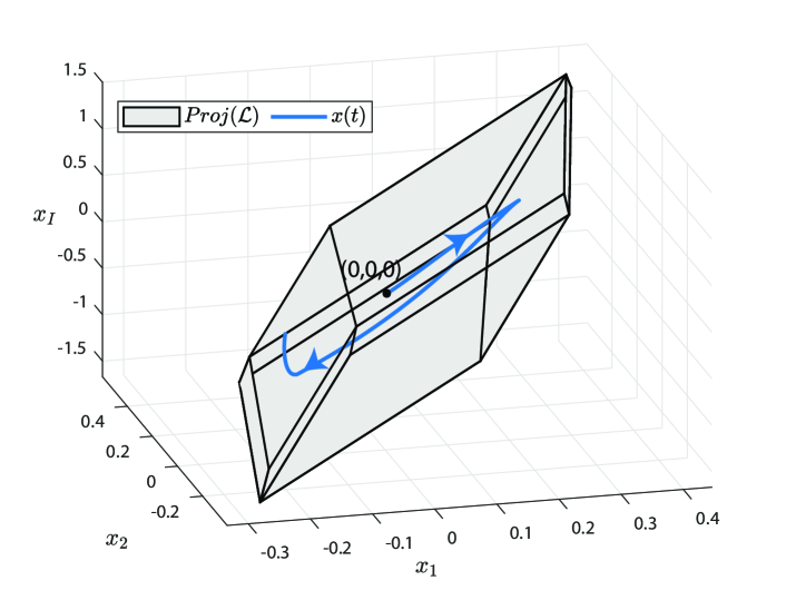
Figure 1: Projected RPI set $\mathcal{L}$ and state trajectory for reference (18)

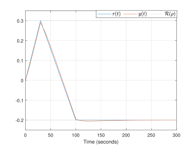
Figure 2: Output and reference tracking for reference (18)

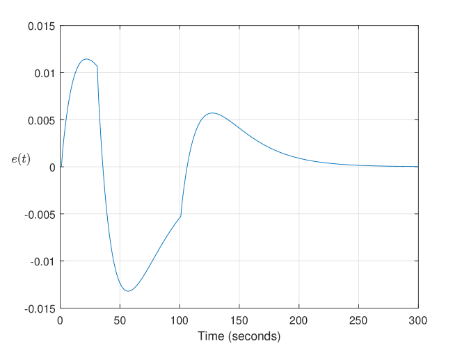
Figure 3: Error signal for reference (18)

Next, we define a sinusoidal signal as a reference input $r=a\sin\omega t$, considering $\omega=1$ and the objective function $\Phi(\cdot)=\Phi_{2}$ in the optimization problem (16). By solving (16), the following results have been obtained: $K=-3.2391$, $K_{I_{1}}=1.6503$, $K_{I_{2}}=-3.1178$, $K_{r}=3.2106$, $X_{I}=\begin{bmatrix}0.1000&-0.1000&0.1000&-0.1000\end{bmatrix}^{T}$ and $a=\rho=0.13$. Fig. 4 shows the projection of the RPI set $\mathcal{L}$ and the trajectory starting from a zero initial condition and following the sinusoidal signal, as shown in Fig. 5, respecting the reference constraints $\mathcal{R}(\rho)$. The error signal shown in Fig. 6 confirms that the proposed controller ensures steady state offset-free tracking of the considered sinusoidal reference signal.

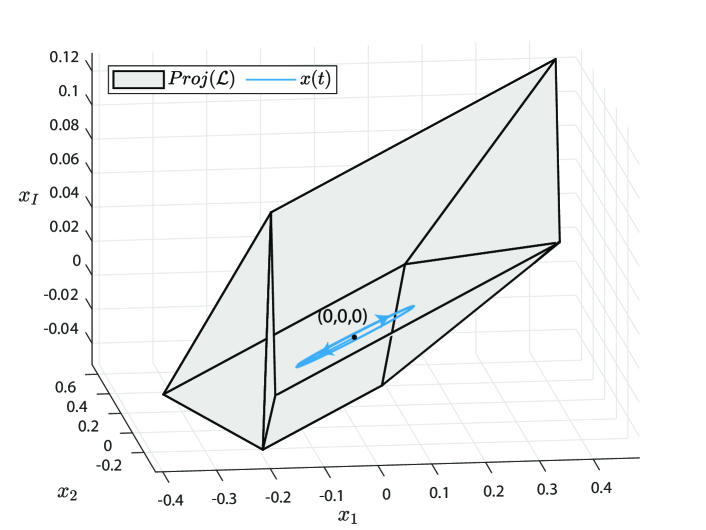
Figure 4: Projected RPI set $\mathcal{L}$ and state trajectory for sinusoidal reference

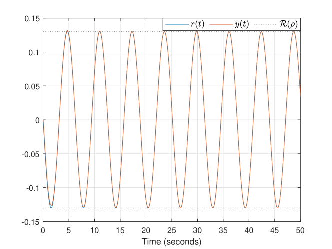
Figure 5: Output and reference tracking for sinusoidal reference

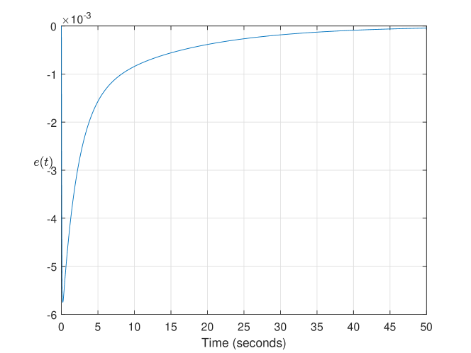
Figure 6: Error signal for sinusoidal reference

V Conclusion

In this paper, we have extended and generalized the approach in [14] to design tracking controllers for constrained linear time-invariant systems whose output is required to track ramp and sinusoidal reference signals. By assuming polyhedral state and input constraints, we have jointly resorted to robust positively invariant sets theory and IMP to define a single bilinear programming problem, which solves the control design problem. The proposed solution can simultaneously compute the controller parameters, the set of admissible reference signals, and the controller’s domain of attraction.

Future works will be devoted to extending the proposed approach to deal with other classes of reference signals and with the possibility that each system output (in multi-output setups) must track a differently-shaped reference trajectory.

Appendix A

This appendix recalls basic definitions for polyhedral sets and the Extended Farkas’ Lemma adapted from [22, 1].

Definition 2

Any closed and convex polyhedral set $\mathcal{P}(\phi)\subseteq\mathbb{R}^{n}$ can be characterized by a shaping matrix $P\in\mathbb{R}^{l_{p}\times n}$ and a vector $\phi\in\mathbb{R}^{l_{p}}$, with $l_{p}$ and $n$ being positive integers, i.e.,

$$\mathcal{P}(\phi)=\{x\in\mathbb{R}^{n}:Px\leq\phi\}.$$ (19)

Note that $\mathcal{P}(\phi)$ in (19) includes the origin as an interior point iff $\phi>0$. In the sequel, if $\phi=\textbf{1}_{*}=[1,\,1,\ldots\,,1\,]^{T}\in\mathbb{R}^{*}$, the resulting polyhedral set $\mathcal{P}(\textbf{1}_{*})$ will be denoted as $\mathcal{P}$.

Definition 3

A matrix $M$ is Metzler type, or essentially non-negative, if $M_{ij}\geq 0,\forall i\neq j$.

Proof of Lemma 1: The existence of the Metzler type matrix $H$, the non-negative matrix $H_{r}$ and the scalar $\gamma>0$ verifying the conditions (12) are necessary and sufficient algebraic conditions for the robust positive invariance of the set $\mathcal{L}$, which is the equivalent of imposing the one step admissibility condition $A_{cl}\mathcal{L}\oplus B_{cl}\mathcal{R}(\rho)\subseteq\mathcal{L}$ (see [23, 24, 1]).

Lemma 2

(Extended Farkas’ Lemma) Consider two polyhedral sets of $\mathbb{R}^{n}$ defined by $\mathcal{P}_{i}(\phi_{i})=\{x\in\mathbb{R}^{n},P_{i}x\leq\phi_{i}\}$, for $i=1,2$, with $P_{i}\in\mathbb{R}^{l_{p_{i}}\times n}$ and positive vectors $\phi_{i}\in\mathbb{R}^{l_{p_{i}}}$. Then, $\mathcal{P}_{1}\subseteq\mathcal{P}_{2}$ if and only if there exists a non-negative matrix $Q\in\mathbb{R}^{l_{p_{2}}\times l_{p_{1}}}$ such that

$$\begin{array}[]{c}QP_{1}=P_{2},\quad Q\phi_{1}\leq\phi_{2}.\end{array}$$ (20)

References

- [1] F. Blanchini and S. Miani, Set-Theoretic Methods in Control, 2nd ed. Springer International Publishing, Birkhäuser, 2015.
- [2] S. Tarbouriech, G. Garcia, J. M. G. da Silva Jr, and I. Queinnec, Stability and stabilization of linear systems with saturating actuators, 1st ed. Springer Science, 2011.
- [3] C. Chen, Linear System Theory and Design, 4th ed., ser. The Oxford Series in Electrical and Computer Engineering. Oxford University Press, 2014.
- [4] B. Carvalho and L. Rodrigues, “Multivariable pid synthesis via a static output feedback lmi,” in IEEE Conference on Decision and Control (CDC). IEEE, 2019, pp. 8398–8403.
- [5] D. Limon, I. Alvarado, T. Alamo, and E. Camacho, “Mpc for tracking of piece-wise constant references for constrained linear systems,” IFAC Proceedings Volumes, vol. 38, no. 1, pp. 135–140, 2005.
- [6] A. Ferramosca, D. Limon, I. Alvarado, T. Alamo, F. Castaño, and E. F. Camacho, “Optimal mpc for tracking of constrained linear systems,” International Journal of Systems Science, vol. 42, no. 8, pp. 1265–1276, 2011.
- [7] S. Di Cairano and F. Borrelli, “Reference tracking with guaranteed error bound for constrained linear systems,” IEEE Transactions on Automatic Control, vol. 61, no. 8, pp. 2245–2250, 2015.
- [8] E. Garone, S. Di Cairano, and I. Kolmanovsky, “Reference and command governors for systems with constraints: A survey on theory and applications,” Automatica, vol. 75, pp. 306–328, 2017.
- [9] J. V. Flores, D. Eckhard, and J. M. G. da Silva Jr, “On the tracking problem for linear systems subject to control saturation,” IFAC Proceedings Volumes, vol. 41, no. 2, pp. 14 168–14 173, 2008.
- [10] L. S. Figueiredo, T. A. R. Parreiras, M. J. Lacerda, and V. J. S. Leite, “Design of lpv-pi-like controller with guaranteed performance for discrete-time systems under saturating actuators,” IFAC Proceedings Volumes, 2020.
- [11] A. N. D. Lopes, V. J. S. Leite, L. F. P. Silva, and K. Guelton, “Anti-windup ts fuzzy pi-like control for discrete-time nonlinear systems with saturated actuators,” International Journal of Fuzzy Systems, vol. 22, no. 1, pp. 46–61, 2020.
- [12] S. Tarbouriech, C. Pittet, and C. Burgat, “Output tracking problem for systems with input saturations via nonlinear integrating actions,” International Journal of Robust and Nonlinear Control, vol. 10, no. 6, pp. 489–512, 2000.
- [13] J. V. Flores, J. M. G. da Silva Jr, and D. Sbarbaro, “Robust periodic reference tracking for uncertain linear systems subject to control saturations,” in IEEE Conference on Decision and Control (CDC). IEEE, 2009, pp. 7960–7965.
- [14] G. A. F. Santos, E. B. Castelan, and W. Lucia, “On the design of constrained pi-like output feedback tracking controllers via robust positive invariance and bilinear programming,” IEEE Control Systems Letters, vol. 7, pp. 1429–1434, 2023.
- [15] G. F. Santos, J. G. Ernesto, E. B. Castelan, and W. Lucia, “Discrete-time constrained pi-like output feedback tracking controllers - a robust positive invariance and bilinear programming approach,” in Simpósio Brasileiro de Automação Inteligente-SBAI, 2023.
- [16] K. J. Åström, T. Hägglund, and K. J. Astrom, Advanced PID control. ISA-The Instrumentation, Systems, and Automation Society Research Triangle Park, 2006, vol. 461.
- [17] R. H. Byrd, J. Nocedal, and R. A. Waltz, “Knitro: An integrated package for nonlinear optimization,” in Large-Scale Nonlinear Optimization, G. Di Pillo and M. Roma, Eds. Boston: Springer, 2006.
- [18] G. A. F. Santos, E. B. Castelan, and J. G. Ernesto, “Pi-controller design for constrained linear systems using positive invariance and bilinear programming,” in IEEE Int. Conference on Automation/XXIV Congress of the Chilean Association of Automatic Control, 2021, pp. 1–7.
- [19] S. L. Brião, E. B. Castelan, E. Camponogara, and J. G. Ernesto, “Output feedback design for discrete-time constrained systems subject to persistent disturbances via bilinear programming,” Journal of the Franklin Institute, vol. 358, no. 18, pp. 9741–9770, 2021.
- [20] J. G. Ernesto, E. B. Castelan, G. A. F. Santos, and E. Camponogara, “Incremental output feedback design approach for discrete-time parameter-varying systems with amplitude and rate control constraints,” in IEEE Int. Conference on Automation/XXIV Congress of the Chilean Association of Automatic Control. IEEE, 2021, pp. 1–7.
- [21] J. K. Martins, F. M. Araújo, and C. E. Dórea, “Um método baseado em otimizaçao para sintonia de controladores pi para sistemas sujeitos a restriçoes,” in Congresso Brasileiro de Automática-CBA, vol. 2, no. 1, 2020.
- [22] J. C. Hennet, “Discrete time constrained linear systems,” Control and Dynamic Systems, vol. 71, pp. 157–214, 1995.
- [23] W. Lucia, J. G. Ernesto, and E. B. Castelan, “Set-theoretic output feedback control: A bilinear programming approach,” Automatica, vol. 153, p. 111004, 2023.
- [24] E. B. Castelan and J. C. Hennet, “On invariant polyhedra of continuous-time linear systems,” IEEE Transactions on Automatic control, vol. 38, no. 11, pp. 1680–1685, 1993.