The minimal seed for transition to convective turbulence in heated pipe flow

Abstract

It is well known that buoyancy suppresses, and can even laminarise turbulence in upward heated pipe flow. Heat transfer seriously deteriorates in this case. A new DNS model is established to simulate the flow and its effect on the flow-dependent heat transfer in an upward heated pipe. The model shows good agreement with experimental results. Three flow states are simulated for different values of the buoyancy parameter $C$: shear turbulence, laminarisation and convective turbulence. The latter two regimes correspond to the heat transfer deterioration regime and the heat transfer recovery regime, respectively (Jackson & Li, 2002; Bae et al., 2005; Zhang et al., 2020). We confirm that convective turbulence is driven by a linear instability (Su & Chung, 2000) and that the deteriorated heat transfer within convective turbulence is related to a lack of near-wall rolls, which leads to a weak mixing between the flow near the wall and centre of pipe. Having surveyed the fundamental properties of the system, we perform a nonlinear nonmodal stability analysis, which seeks the minimal perturbation that triggers a transition from the laminar state. Given the differences between shear-driven and convection-driven turbulence, we aim to determine how the nonlinear optimal (NLOP) changes as the buoyancy parameter $C$ increases. We find that, at first, the NLOP becomes thinner and closer to the wall. Most importantly, the critical initial energy $E_{0}$ required to trigger turbulence keeps increasing, implying that attempts to artificially trigger it may not be an efficient means to improve heat transfer at larger C. At a larger $C=6$, a new type of NLOP is discovered, capable of triggering convective turbulence from lower energy, but over longer time. It is active only in the centre of pipe. We next compare the transition processes from linear instability and by the nonlinear nonmodal excitation. At $C=4$, linear instability leads to a state that approaches a travelling wave solution or periodic solutions, while the minimal seed triggers shear-turbulence before decaying to convective turbulence. Deeper into the parameter space for convective turbulence, at $C=6$, the new nonlinear optimal triggers convection-driven turbulence directly. Detailed analysis of the periodic solution reveals three stages: growth of the unstable eigenfunction, the formation of streaks and the decay of the streaks. The stages of the cycle correspond to changes in the linear instability of turbulent mean velocity profile. Unlike for classical shear flows, where the streak is disrupted via instability, here decay of the streak is more closely linked to suppression of the linear instability of the mean flow, and hence suppression of the rolls. Flow visualizations at $C$ up to $10$ also show similar processes, suggesting that convective turbulence in the heat transfer recovery regime is sustained by these three typical processes.

1 Introduction

In isothermal pipe flow, the flow is driven by an external pressure gradient. This is referred to as ‘forced’ flow. In a vertical configuration, however, buoyancy resulting from the lightening of the fluid close to a heated wall can provide a force that partially or fully drives the flow, referred to as ‘mixed’ or ‘natural convection’ respectively. Employing mixed convection is fundamental and practical in engineering applications, e.g. geothermal energy capture, nuclear reactor cooling systems, fossil-fuel power plants, and so on, which has been widely researched. Heat transfer in the presence of buoyancy exhibits totally different characteristics for downward flow and upward flow. In a downward flow, the buoyancy acts as a drag force but always enhances the heat transfer. Conversely, in an upward flow, the buoyancy assists the flow, but the heat transfer can be significantly deteriorated (McEligot et al., 1970; Ackerman, 1970; Bae et al., 2005; Wibisono et al., 2015; Zhang et al., 2020). When the heating parameter is gradually increased, the heat transfer first deteriorates, then recovers and eventually approaches the same values as a downward flow (Zhang et al., 2020). As for the flow characteristics, interestingly, shear turbulence is gradually suppressed and even laminarised at a lower Reynolds numbers (Bae et al., 2005; He et al., 2016; Chu et al., 2016; He et al., 2021), then the flow comes into a convective turbulence state when the buoyancy exceeds a critical intensity (Su & Chung, 2000; Marensi et al., 2021).

Research on the phenomenon of laminarisation in mixed convection can be traced at least as far back as Hall & Jackson (1969), who provided a theoretical explanation of this phenomenon, suggesting that reduced shear stress in the buffer layer leads to a reduction or even elimination of turbulence production. This interpretation obtained wide acceptance. More recently, He et al. (2016) modelled the buoyancy with a radially-dependent body force added to the isothermal case, successfully reproducing the laminarisation phenomena. They found that the body force causes little change to the key characteristics of turbulence, and proposed that laminarisation is caused by the reduction of so called ‘apparent Reynolds number’, which is calculated based only on the pressure force of the flow (i.e. excluding the contribution of the body force). In flows at supercritical pressure, the heat transfer and flow characteristics are very similar to the normal flow, the laminarisation and heat transfer deterioration are successfully reproduced by Bae et al. (2005, 2006). He et al. (2021) researched the laminarisation phenomenon in flows at supercritical pressure, and a unified explanation was established for the laminarisation mechanisms. It is thought to be due to the variations of thermophysical properties, buoyancy and inertia, the last of which plays a significant role in a developing flow.

Meanwhile in isothermal flow, the laminarisation phenomenon has been observed when the base velocity profile is flattened (Hof et al., 2010; Kühnen et al., 2018; Marensi et al., 2019), which is quite similar to the effect of buoyancy on the base velocity profile. Kühnen et al. (2018) proposed that the laminarisation is caused by the reduced transient growth when the velocity profile is flattened. Marensi et al. (2019) considered the nonlinear stability of a series of flattened base velocity profiles in (isothermal) pipe flow, and found that the flattening enhances the nonlinear stability of the laminar flow. Recently, machine learning has been used to explore laminarisation events in a reduced model of wall-bounded shear flows, and it has been suggested that the collapse of turbulence is connected with the suppression of streak instabilities (Lellep et al., 2022).

There have been many studies of mixed convection, both experimental (Celataa et al., 1998; Wang et al., 2011; Jackson, 2013; Zhang et al., 2020) and numerical (You et al., 2003; Poskas et al., 2012; Yoo, 2013; Zhao et al., 2018), but most of these works focus on statistical properties, e.g. the Nusselt number, Reynolds stress, mean velocity profile, the mean temperature profile and so on. Few works pay attention to the dynamical characteristics of the flow, such as transition between flow types and maintenance of convective turbulence. In particular, the transition mechanisms of mixed convection appear to be quite different from those of the isothermal flow. Experimental results (Hanratty et al., 1958; Scheele et al., 1960; Ackerman, 1970) have shown that a heated vertical pipe flow can go through a flow transition at Reynolds number as low as $30$. Scheele & Hanratty (1962) found that the vertical heated upflow in a pipe first becomes unstable when the velocity profiles develop an inflectional point. The flow comes into a regular and periodic motion after transition at rather low Reynolds number. Similar patterns have been also observed by Kemeny & Somers (1962). Yao (1987) confirmed the experimental observations that the flow in a heated vertical pipe is supercritically unstable. They found the bifurcated new equilibrium laminar flow is likely to be a double spiral flow. A weakly nonlinear instability analysis by Rogers & Yao (1993) revealed that the heated upflow is supercritically unstable while heated downflow is potentially subcritically unstable. Su & Chung (2000) systematically researched the linear stability of mixed-convection upward and downward flow in a vertical pipe with constant heat flux, to explain the multiple flow states that appeared in the experimental and numerical results. The calculation found that the first azimuthal mode is always the most unstable. The Rayleigh-Taylor instability is operative when the Reynolds number is extremely low, while the opposed-thermal-buoyant instability is dominant when the Reynolds number is higher. The transition of a low Reynolds number mixed-convection flow in a vertical channel was investigated by Chen & Chung (2002) for both K-type (Klebanoff et al., 1962) and H-type (Herbert, 1983) disturbances. It was found that the flow field bifurcates to a new quasi-steady nonlinear state after the initial transient period, for both types of perturbation. Khandelwal & Bera (2015) developed a weakly nonlinear stability theory in terms of a Landau equation to analyse the nonlinear saturation of stably stratified non-isothermal Poiseuille flow in a vertical channel with respect to different fluids, i.e. mercury, gases, liquids and heavy oils. A substantial enhancement in heat transfer rate was found for liquids and heavy oils from the basic state beyond the critical Rayleigh number. Recently, Marensi et al. (2021) also performed linear stability analysis for a vertical heated pipe flow, using the parameter $C$ to measure the buoyancy force relative to the force that drives the laminar isothermal shear flow. Their results show that the flow is not always linearly unstable at a strong buoyancy condition, and revealed that the heat transfer deterioration is caused by the suppression of rolls in the flow. This finding is in line with the study of Lellep et al. (2022), as suppression of rolls would occur when streak instabilities are suppressed.

Some works have considered the linear and weakly nonlinear stability of a vertical heated flow, and have shown the instability to convective turbulence. However, the transition involving shear-driven turbulence is fundamentally nonlinear, and multiple flow states can arise at the same parameter values. Further understanding is of great significance for heat transfer prediction and optimisation in engineering applications, and there remain open questions to be addressed, e.g.: How does the shear turbulence gradually disappear? Is laminarisation similar to that in isothermal flow? How is the convective turbulence triggered and sustained?

To tackle these questions, we employ nonlinear nonmodal stability analysis (Pringle & Kerswell, 2010; Cherubini et al., 2011; Pringle et al., 2012; Cherubini & De Palma, 2013; Marensi et al., 2019) to seek the most efficient perturbation to trigger transition from the laminar state in a vertical heated pipe. The optimised perturbation is called the nonlinear optimal (NLOP), and the critical (i.e. lowest energy) NLOP that triggers turbulence has been dubbed the ‘minimal seed’ in isothermal flow. The minimal seed can reflect the nonlinear stability of the flow to some extent (Marensi et al., 2019). The Lagrange multiplier method has been widely used in fluid mechanics, including the heat transfer optimisation approach proposed by Guo et al. (2007); Motoki et al. (2018). We do not optimise heat transfer directly here, however, but seek the optimal flow perturbation that leads to transition away from the low heat-transfer state of laminar flow.

The plan of the paper is as follows. In §2, we present the new model for direct numerical simulation (DNS) of vertical heated pipe flow, and equations of the linear stability and nonlinear nonmodal stability analysis. In §3, we firstly show the DNS results, then present the results of linear stability and nonlinear nonmodal stability analysis, and lastly we reveal the transition processes by NLOP and unstable eigenfunctions, as well as the self-sustaining process in convective turbulence. Finally, the paper concludes with a summary in §4.

2 Formulation

2.1 Simulation of heated pipe flow

Like several models, we assume there is a background temperature gradient along the axis of the pipe, e.g. Yao (1987); Chen & Chung (1996, 2002); Khandelwal & Bera (2015). Different from many models, however, we suppose that the temperature gradient may vary in time: we fix the difference between the bulk temperature of the fluid and that of the wall, aiming to see directly how the buoyancy parameter affects the flow pattern, and hence the heat flux at the wall and the temperature gradient. Our code is a modification to that of Marensi et al. (2021), wherein a spatially uniform heat sink was assumed. Let $\boldsymbol{x}=(r,\theta,z)$ denote cylindrical coordinates. We decompose the total temperature as $T_{tot}(\boldsymbol{x},t)=T_{w}(z,t)+T(\boldsymbol{x},t)-\Delta T$, with wall temperature $T_{w}=a(t)z+b$, for some constant reference temperature $b$. Axial periodicity over a distance $L$ is assumed for the fluctuation field $T$ and velocity field $\boldsymbol{u}_{tot}$. Now let $T_{b}=\langle T\rangle$, where the angle brackets denotes the spatial average. To ease interpretation a little for the heated pipe case, the temperature scale $\Delta T=2\,T_{b}$ has been inserted so that the local temperature fluctuations $T$ are positive and greatest at the wall, where they satisfy $T=\Delta T$. We take $\Delta T$ as our temperature scale for non-dimensionalisation, and assume that local fluctuations in $T$ are more rapid than changes in the gradient $a(t)$. For the length and velocity scales, we use the radius $R$ and twice the bulk flow speed, $2U_{b}$, the latter of which coincides with the isothermal laminar centreline speed. Throughout the rest of the text, dimensionless variables and equations are presented.

Temperature fluctuations $T$ satisfy

$$\frac{\partial T}{\partial t}+({\boldsymbol{u}_{tot}}\cdot\boldsymbol{\nabla})T=\frac{1}{RePr}\boldsymbol{\nabla}^{2}T-{\boldsymbol{u}_{tot}}\bcdot{\hat{\boldsymbol{z}}}\,a(t)$$ (1)

with boundary condition $T=1$ at the wall. A fixed bulk temperature, $\langle T\rangle=1/2$, is maintained through adjustments in the gradient $a(t)$. The dimensionless parameters are $Re=2U_{b}R/\nu$ and $Pr=\nu/\kappa$, where $\nu$ and $\kappa$ are the kinematic viscosity and thermal diffusivity respectively. Under the Boussinesq approximation (Turner & Turner, 1979), the Navier–Stokes (NS) equations are

$$\frac{\partial\boldsymbol{u}_{tot}}{\partial t}+(\boldsymbol{u}_{tot}\bcdot\boldsymbol{\nabla}){\boldsymbol{u}_{tot}}=-\boldsymbol{\nabla}p_{tot}+\frac{1}{Re}\boldsymbol{\nabla}^{2}{\boldsymbol{u}_{tot}}+\frac{4}{Re}(1+\beta^{\prime}(t)+CT)\hat{\boldsymbol{z}}$$ (2)

with continuity equation

$$\boldsymbol{\nabla}\cdot\boldsymbol{u}_{tot}=0.$$ (3)

and no-slip condition $\boldsymbol{u}=\boldsymbol{0}$ at the wall. Here, $\beta^{\prime}(t)$ is the excess pressure fraction, relative to isothermal laminar flow, required to maintain fixed dimensionless mass flux, $\langle{\boldsymbol{u}_{tot}}\cdot{\hat{\boldsymbol{z}}}\rangle=1/2$. The dimensionless parameter

$$C=\frac{Gr}{16\,Re}$$ (4)

measures the buoyancy force relative to the force that drives laminar isothermal shear flow, where $G_{r}={\gamma g(T_{w}-T_{b})D^{3}}/{\nu^{2}}$ is the Grashof number. For further details, see Marensi et al. (2021).

As the focus of this study is on the dynamics of perturbations from the laminar solution, we decompose the variables, ${\boldsymbol{u}_{tot}}=\boldsymbol{u}_{0}+\boldsymbol{u}$, $p_{tot}=p_{0}+p$, $1+\beta^{\prime}(t)=1+\beta_{0}+\beta(t)$, $T=\Theta_{0}+\Theta$, $a_{tot}(t)=a_{0}+a(t)$, where subscript $0$ tags the laminar solution. The laminar velocity $\boldsymbol{u}_{0}=u_{0}(r)\,\hat{\boldsymbol{z}}$ satisfies

$$-\boldsymbol{\nabla}p_{0}+\frac{1}{Re}\boldsymbol{\nabla}^{2}{\boldsymbol{u}_{0}}+\frac{4}{Re}(1+\beta_{0}+C\Theta_{0})\hat{\boldsymbol{z}}=0$$ (5)

Subtracting (5) from (2), we obtain

$$\frac{\partial\boldsymbol{u}}{\partial t}+u_{0}\frac{\partial\boldsymbol{u}}{\partial z}+u_{r}\,\frac{du_{0}}{dr}\,\hat{\boldsymbol{z}}+\boldsymbol{u}\bcdot\boldsymbol{\nabla}\boldsymbol{u}=-\boldsymbol{\nabla}p+\frac{1}{Re}\boldsymbol{\nabla}^{2}\boldsymbol{u}+\frac{4}{Re}(C\Theta+\beta)\hat{\boldsymbol{z}}.$$ (6)

The laminar temperature profile $\Theta_{0}(r)$ satisfies

$$\frac{1}{RePr}\boldsymbol{\nabla}^{2}\Theta_{0}=\boldsymbol{u}_{0}\bcdot{\hat{\boldsymbol{z}}}a_{0}.$$ (7)

Subtracting (7) from (1), we obtain

$$\frac{\partial\Theta}{\partial t}+u_{0}\frac{\partial\Theta}{\partial z}+u_{r}\frac{d\Theta_{0}}{dr}+(\boldsymbol{u}\bcdot\boldsymbol{\nabla})\Theta=\frac{1}{RePr}\boldsymbol{\nabla}^{2}\Theta-u_{z}a_{0}\boldsymbol{\hat{z}}-(u_{0}+u_{z})a(t)\boldsymbol{\hat{z}}.$$ (8)

Taking the spatial average of (8) provides an equation to determine the value of $a(t)$ required to maintain fixed bulk temperature of the perturbation $\langle\Theta\rangle=0$,

$$a(t)=2\langle N\rangle+\frac{4}{RePr}\left.\partial_{r}\Theta_{00}\right|_{r=1},$$ (9)

where $N$ is the nonlinear terms on the left-hand side of (8) and the subscript $00$ corresponds to averaging over $\theta$ and $z$.

2.2 Linear stability analysis

Arnoldi iteration is employed to calculate the leading eigenvalues and eigenfunctions of the laminar solution using our simulation code. Considering a small perturbation $\boldsymbol{u}$ to the laminar solution $u_{0}$, the system can be simplified as

$$\partial_{t}\boldsymbol{u}=A(u_{0})\boldsymbol{u}\,.$$ (10)

Integrating over a period $T$, eigenfunctions of (10) with growth rate $\sigma$ satisfy the exponentiated eigenvalue problem

$$\mathrm{e}^{\sigma T}\boldsymbol{u}=\boldsymbol{u}+\int_{0}^{T}A(u_{0})\boldsymbol{u}=B(u_{0})\boldsymbol{u}\,.$$ (11)

The Arnoldi method only requires the result of calculations of multiplies by $B$ with given $\boldsymbol{u}$, without needing to know the matrix $B$ itself. Given a starting $\boldsymbol{u}_{0}$, the method seeks eigenvectors in $\mathrm{span}\{\boldsymbol{u}_{0},B\boldsymbol{u}_{0},B^{2}\boldsymbol{u}_{0},...\}$, using Gram-Schmidt orthogonalisation to improve the numerical suitability of this basis set. Using $f(\boldsymbol{u})$ to denote the result of time integration of a perturbation $\boldsymbol{u}$, we may make the approximation

$$B(u_{0})\boldsymbol{u}\approx\frac{1}{\epsilon}\left\{f(\boldsymbol{0}+\epsilon\boldsymbol{u})-f(\boldsymbol{0})\right\}~{}=~{}\frac{1}{\epsilon}f(\epsilon\boldsymbol{u})\,,$$ (12)

for some small value $\epsilon$.

2.3 Nonlinear nonmodal stability analysis

When the linear system is stable, we must appeal to the nonlinear dynamics of the flow. The NLOP (Pringle & Kerswell, 2010; Pringle et al., 2012), which is the optimal perturbation that achieves the largest energy growth, can provide information on the transition dynamics of a linearly stable system.

The NLOP can be found by Lagrange multiplier technique, for details see Pringle et al. (2012). To reduce complexity, we consider only the optimal velocity perturbation, and set the initial temperature perturbation to zero. In this case, the Lagrangian is defined by

$$\begin{split}\mathcal{L}=\langle\frac{1}{2}(\boldsymbol{u}(x,T))^{2}\rangle\mathrm{d}t-\lambda(\frac{1}{2}\langle(\boldsymbol{u})^{2}\rangle-E_{0})-\int_{0}^{T}\langle\boldsymbol{v}(\mathrm{NS}(\boldsymbol{u}))\rangle\mathrm{d}t-\\ \int_{0}^{T}\langle\Pi(\boldsymbol{\nabla}\bcdot\boldsymbol{u})\rangle\mathrm{d}t-\int_{0}^{T}\langle\pi(\mathrm{Tem}(\Theta))\rangle\mathrm{d}t-\\ \int_{0}^{T}\langle\Gamma(\boldsymbol{u}\bcdot\hat{\boldsymbol{z}})\rangle\mathrm{d}t-\int_{0}^{T}\langle Q(\Theta)\rangle\mathrm{d}t\end{split}$$ (13)

Here, $\mathrm{NS}(u)$ and $\mathrm{Tem}(\Theta)$ represent the Navier–Stokes equations and temperature equation. Taking variations of $\mathcal{L}$ with respect to each variable and setting them equal to zero, we obtain the following sets of Euler–Lagrange equations for turbulent field. The adjoint Navier–Stokes, temperature equation and continuity equations are

$$\begin{split}\frac{\partial\mathcal{L}}{\partial\boldsymbol{u}}=\frac{\partial\boldsymbol{v}}{\partial t}+u_{o}\frac{\partial\boldsymbol{v}}{\partial z}-v_{z}{u_{o}}^{\prime}{\hat{\boldsymbol{r}}}+\boldsymbol{\nabla}\times(\boldsymbol{v}\times\boldsymbol{u})-\boldsymbol{v}\times\boldsymbol{\nabla}\times\boldsymbol{u}+\boldsymbol{\nabla}\Pi+\\ \frac{1}{Re}\boldsymbol{\nabla}^{2}\boldsymbol{v}-\pi\Theta_{o}^{\prime}\hat{\boldsymbol{r}}-\pi\boldsymbol{\nabla}\Theta-\pi(a(t)+a_{0}(t))\hat{z}-\mathcal{T}\hat{\boldsymbol{z}}=0\end{split}$$ (14)

$$\frac{\partial\mathcal{L}}{\partial\Theta}=\frac{\partial\pi}{\partial t}+u_{o}\frac{\partial\pi}{\partial z}+\frac{4}{Re}v_{z}C+\boldsymbol{u}\bcdot\boldsymbol{\nabla}\pi+\frac{1}{RePr}\boldsymbol{\nabla}^{2}\pi-Q=0$$ (15)

$$\frac{\delta\mathcal{L}}{\delta p}=\boldsymbol{\nabla}\bcdot\boldsymbol{v}=0$$ (16)

The compatibility condition is given by

$$\frac{\delta\mathcal{L}}{\delta\boldsymbol{u}(x,T)}=\boldsymbol{u}(x,T)-\boldsymbol{v}(x,T)=0$$ (17)

$$\frac{\delta\mathcal{L}}{\delta\Theta(x,T)}=-\pi(x,T)=0.$$ (18)

and the optimality condition is

$$\frac{\delta\mathcal{L}}{\delta{\boldsymbol{u}(x,0)}}=-\lambda\boldsymbol{u}(x,0)+\boldsymbol{v}(x,0)=0.$$ (19)

As the optimality condition is not satisfied automatically, $\boldsymbol{u}(x,0)$ is moved in the direction of $\delta\mathcal{L}/\delta\boldsymbol{u}(x,0)$ to achieve a maximum where $\delta\mathcal{L}/\delta\boldsymbol{u}(x,0)$ should vanish. The maximisation problem is solved numerically using an iterative algorithm similar to that applied in Pringle et al. (2012); Marensi et al. (2019). The update for $\boldsymbol{u}(x,0)$ at $(j+1)\mathrm{th}$ iteration is

$$\boldsymbol{u}(x,0)^{(j+1)}=\boldsymbol{u}(x,0)^{(j)}+\epsilon\frac{\delta\mathcal{L}}{\delta\boldsymbol{u}(x,0)^{(j)}}.$$ (20)

The $\lambda$ is used to set $\langle[\boldsymbol{u}(x,0)^{(j+1)}]^{2}\rangle=E_{0}$, and $\epsilon$ is a small number, controlled as in Pringle et al. (2012) to aid convergence.

2.4 Time integration code

The calculations are carried out by the open source code openpipeflow.org (Willis, 2017). At each time step, the unknown variables, i.e. the velocity and pressure perturbations ${\boldsymbol{u},p}$ are discretised in the domain $\left\{r,\theta,z\right\}=[0,1]\times[0,2\pi]\times[0,2\pi/k_{0}]$, where $k_{0}=2\pi/L$, using Fourier decomposition in the azimuthal and streamwise direction and finite difference in the radial direction

$$\left\{\boldsymbol{u},p,\Theta\right\}(r_{s},\theta,z)=\sum_{k<|K|}\sum_{m<|M|}\left\{\boldsymbol{u},p,\Theta\right\}_{skm}e^{i(k_{0}kz+m\theta)}$$ (21)

where $s=1,...,S$ and the radial points are clustered close to the wall. Temporal discretisation is via a second-order predictor-corrector scheme, with an Euler predictor and Crank-Nicolson corrector applied to the nonlinear terms. The laminar solution is quickly calculated by eliminating azimuthal and axial variations, using a resolution $S=64,M=1,K=1$. As the adjoint optimisation requires forwards and backwards time integrations each iteration, it is computationally expensive. To keep the calculations manageable, a Reynolds number $Re=3000$ is adopted for the nonlinear nonmodal stability analysis with a domain of length $L=5D$. We use $S=64,M=48,K=42$ and a time step $\Delta t=0.01$.

3 Results

3.1 Flow regimes

Figure 1 shows how the laminar velocity and temperature profile changes with $C$. It can be clearly observed that the velocity profile becomes flattened and is well known to become ‘M-shaped’ at larger values of $C$. The temperature profile also changes, but not so strongly. The boundary temperature gradient of laminar state is shown in figure 2$(a)$. With the increase of buoyancy, the temperature gradient increases a little, while the temperature gradient decreases as $\Rey$ is increased, as the higher flow speed takes heat out of the system more quickly. The Nusselt number is defined as

$$N_{u}=\frac{q_{w}\,D}{\lambda(T_{w}-T_{b})}\,,$$ (22)

where $\lambda$ is thermal conductivity of fluid, $q_{w}$ is net wall heat flux. Clearly, the laminar Nusselt number increases with a larger value of $C$, see figure 2$(b)$, but it is independent of the Reynolds number (Su & Chung, 2000).

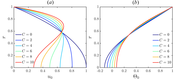
Figure 1: ($a$) the laminar velocity profile, ($b$) the laminar temperature profile. Laminar profiles are independent of Reynolds number.

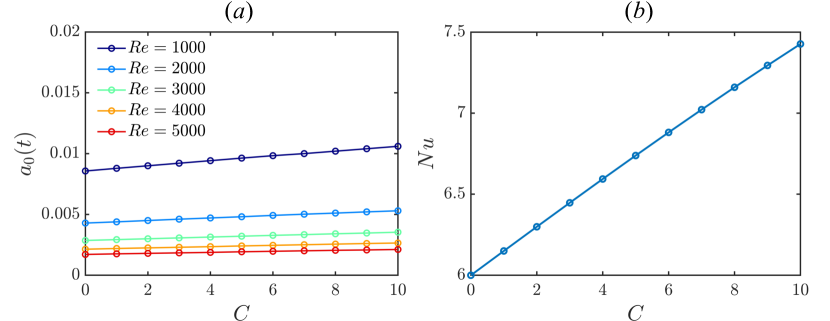
Figure 2: ($a$) Temperature gradient of laminar flow as a function of $C$ for several$\Rey$. ($b$) Nusselt number as a function of $C$.

As discussed in the introduction, there are three typical flow states: the laminar flow, shear turbulence, and convective turbulence. We performed simulations at different Reynolds number $\Rey$ and buoyancy parameter $C$ and report the observed regime of flow state in figure 3$(a)$. The diagram is consistent with figure 7 of Marensi et al. (2021). Although the flow near the boundary with shear turbulence may be in either of two flow states, three typical flow regimes can be identified clearly. In the iso-thermal case ($C=0$) , the flow is shear-driven turbulence at $Re>2040$ (Avila et al., 2011, 2023), but increasing the effect of buoyancy, at lower Reynolds number, the flow first laminarises then transitions to convective turbulence. At a higher Reynolds number, the laminarisation regime becomes narrower and finally disappears. Convective turbulence first appears for $C\gtrsim 4$, at lower Reynolds number, as reported by Scheele et al. (1960); Scheele & Hanratty (1962); Yao (1987). But at high Reynolds number, there is a crossover with the shear-driven state, and the critical $C$ for switch to convective turbulence increases.

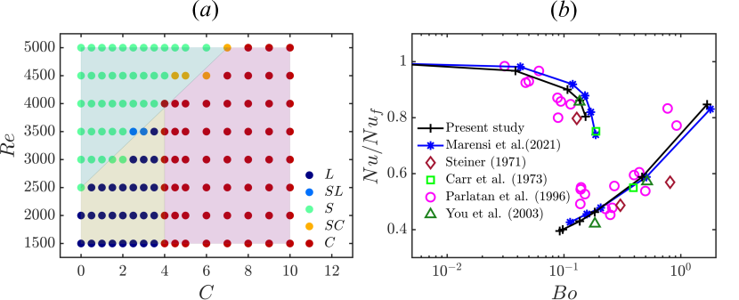
Figure 3: $(a)$ Regions of laminar flow (L), shear turbulence (S) and convection flow (C). SL and SC indicate that the flow may be in either of the two states. $(b)$ Change in heat flux, normalised by that for isothermal state ($C\to 0$), as a function of $Bo=8\times 10^{4}\,(8\,Nu\,Gr)/(\Rey^{3.425}Pr^{0.8})$. Data from simulations at $Re=5300$, $Pr=0.7$ and various $Gr=16ReC$. The upper and lower branches correspond to flow in shear-driven and convection-driven states, respectively.

The numerical results are quantitatively validated by comparison with experiments, shown in figure 3$(b)$, which also includes the numerical results of Marensi et al. (2021). The strong heat flux for smaller values of buoyancy number $Bo=8\times 10^{4}\,(8\,Nu\,Gr)/(\Rey^{3.425}Pr^{0.8})$ is brought by shear turbulence, but deteriorates with the increase of $Bo$, due to the suppression of shear turbulence by the buoyancy force. When the buoyancy force exceeds a certain level, the flow switches from shear turbulence to convective turbulence, accompanied by a sudden drop of heat transfer. But the heat transfer recovers with a further increase of buoyancy. The captured heat transfer features are consistent with the results reported by Bae et al. (2005); Yoo (2013). In the present model, the velocity field is allowed to affect the heat flux at the wall; the model and code are a minor update to that of Marensi et al. (2021). Their model, however, assumed a constant boundary temperature with a spatially uniform heat sink term. That has the advantage that there is a simple analytic expression for the laminar base flow, but the axial temperature gradient which leads to the spatially dependent heat sink term is expected to be closer to the real system. Compared with Marensi et al. (2021), it is found that the present model provides a small improvement in agreement with experimental data in the shear-turbulence regime, while in the convection turbulence regime the two models give similar results.

Figure 4 shows the effect of the switch between flow states at $Re=3000$ for $C=1,3,5$. When the buoyancy is weak, at $C=1$, in figure 4($a$), we find that all three components of the energy maintain a high amplitude. The flow is essentially unchanged from the shear turbulence at $C=0$. When $C=3$, the velocity perturbation energy decays quickly, indicating the occurrence of laminarisation. At $C=5$, as similar energy drop is also observed, but stops at a lower energy level and fluctuates with a low frequency, which is typical of the convective turbulent state. The heat transfer in the laminar and convective turbulent state is severely reduced, see figure 4($b$), where the Nusselt number drops to half of that in shear turbulence. The convective turbulent state at these parameters has a Nusselt number that is not much greater than for the laminar state.

Iso-surfaces of the streamwise vorticity are plotted in figure 5 for shear turbulence $(C=1)$ and convective turbulence $(C=5)$. The shear turbulence has complicated streamwise vortices that fill the whole pipe, while the convective turbulence is made of more organised vortex structures, which are mainly concentrated in the middle of the pipe. The location of the structures can be seen more clearly in the cross-sections of figure 6. In shear turbulence there are abundant near-wall streamwise vortices, which lift up low-speed streaks, and enhance the mixing of fluid in the pipe. While in convective turbulence the perturbation mainly concentrates on the centre of the pipe, the flow near wall is almost steady. There are almost no near-wall rolls and streaks observed. Further visualisations of flow at larger $C$ show similar characteristics. The self-sustaining process of shear turbulence, reliant on near-wall vortices for the creation of streaks, has been destroyed in convective turbulence. The lack of streamwise vortices significantly weakens the interaction between fluid near the wall and center, and heat transfer is therefore seriously damaged.

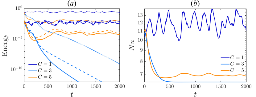
Figure 4: Simulation at $Re=3000$ starting from the same initial condition at $C=1,3,5$. ($a$) Velocity perturbation energy. The dotted, dash and solid line represent the energy of three components of velocity, marked as $E(u_{r})$, $E(u_{t})$ and $E(u_{z})$, respectively. ($b$) Nusselt number.

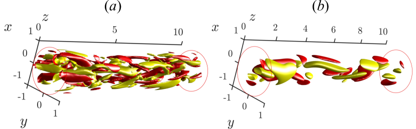
Figure 5: The iso-surface of streamwise vorticity at ($a$)$C=1$ and ($b$) $C=5$ at $Re=3000$, red/yellow are $30\%$ of the mini/max streamwise vorticity.

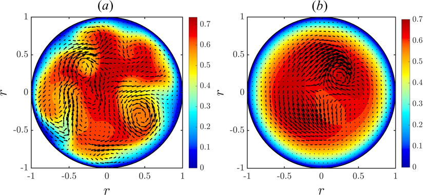
Figure 6: The cross section of ($a$)$C=1$ and ($b$) $C=5$ at $Re=3000$, the contours are colored by streamwise total velocity, the arrows represent cross-stream components. The largest arrow has magnitude $5.6e-3$ in $(a)$ and $1.93e-4$ in $(b)$.

3.2 Linear stability results

This section examines the change of linear stability of the laminar solution at different $C$, revealing how the buoyancy affects the dynamics near the laminar solution. Time stepping is combined with Arnoldi iteration to calculate the leading eigenvalues and eigenfunctions for small perturbations about the laminar state. A resolution of $S=64,M=10,K=10$ is used, which allows the algorithm to pick the most unstable axial and azimuthal modes possible in the given domain ($L=5D$). It is found that the most unstable mode is always of azimuthal wavenumber $m=1$ and is usually of wave number $k=1$ or $k=2$. These observations are consistent with results of Scheele et al. (1960); Su & Chung (2000); Marensi et al. (2021). The real part of eigenvalue of the unstable modes are shown in figure 7. The instability first appears near $C=4$, consistent with the appearance of convective turbulence, verifying the convective turbulence is caused by linear instability (Yao, 1987; Rogers & Yao, 1993; Marensi et al., 2021). Two types of unstable mode lead the instability of the flow, but their growth always remains a small value, even at the larger $C$ considered. The eigenvalues present some complex trends, but for $Re\geq 2000$ the trends are mostly similar. Interestingly, the flow is not always linearly unstable for $C>4$, as there is a small window of stability for $C\approx 5-6$ for a range of $\Rey$. This was also reported for the model of Marensi et al. (2021). For example, at $Re=3000$ the flow is linearly stable for $C=6$. Note that we will take advantage of this for the nonlinear stability analysis of the following subsection §3.3.

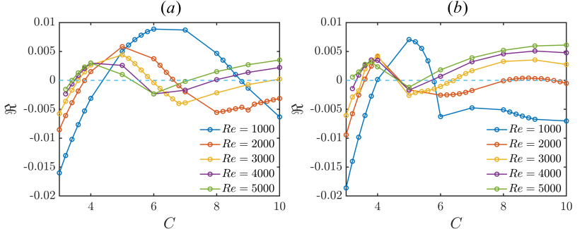
Figure 7: Growth rate of perturbations of different streamwise wave number at several Reynolds number ($a$) $m=1,k=1$ ; ($b$) $m=1,k=2$.

The eigenfunctions of two unstable modes ($m=1,k=1$ and $m=1,k=2$) are shown in figure 8, by the iso-surface of streamwise velocity and streamwise vorticity. The eigenfunctions are consistent with results of Khandelwal & Bera (2015); Marensi et al. (2021). The perturbation is mainly active in the centre of pipe, which is consistent with observation of Su & Chung (2000); Marensi et al. (2021). It can be observed that this kind of unstable mode can produce a pair of streamwise vortices in the centre, and a pair of thin streamwise vortices near the wall, see figure 8$(c,d)$. The streamwise vortices in the centre cannot enhance the mixing of low-speed flow near the wall and high-speed flow in the centre, while the near wall streamwise vortices are also too weak and too thin to assist heat transfer. As a result, the heat transfer in convective turbulence regime remains weak.

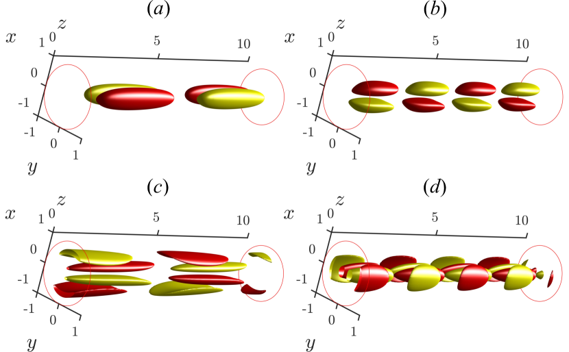
Figure 8: The iso-surface of streamwise velocity perturbation ($a,c$)$m=1,k=1$ , and streamwise vorticity ($b,d$) $m=1,k=2$, of first two unstable eigenfunctions at $C=4,Re=3000$ (red/yellow are 30$\%$ of the min/max streamwise velocity perturbation).

Linear stability analysis results have confirmed that convective turbulence is triggered by linear instability, thus it mainly appears at $C>4$ as shown by the magenta shadowed region in figure 3$(a)$. However, at high Reynolds number, the critical $C$ for transition moves to larger $C$. This indicates a competition between shear turbulence and convective turbulence. For the laminarisation phenomenon shown in the yellow shadowed region in figure 3$(a)$, different possible explanations have been proposed. He et al. (2016) linked the buoyancy-modified flow to a partner isothermal flow at a different (lower) ‘apparent Reynolds number’, based on an apparent friction velocity associated with only the pressure force of the flow (i.e. excluding the contribution of the body force). They found that the buoyancy can reduce the apparent Reynolds number, thereby suppressing turbulence. Kühnen et al. (2018) suggested that it is the flattened base velocity profile, see figure 1, which reduces the transient growth of streaky perturbations, and thereby causes the laminarisation. Marensi et al. (2019) did a nonlinear non-normal stability analysis of the flattened base velocity profile, suggesting the nonlinear stability of the flattened velocity profile is enhanced, i.e. a larger amplitude perturbation is required to trigger turbulence. Lellep et al. (2022) used a machine learning method and linked the collapse of turbulence to the suppression of streak instability. We hold a similar view to Lellep et al. (2022) — through linear and nonlinear optimisation, we have found that a body force which flattens the base velocity profile always shapes more stable streaks. Further numerical experiments have been carried out, imposing a body force which flattens the base velocity profile at particular times during the relative periodic orbit, i.e. only during the time interval of the formation of streaks, or the interval for the regeneration of rolls. Only when targeting the formation of streaks was the self-sustaining process disrupted, supporting that the flattened profile suppresses turbulence by the stabilisation of streaks (Chu et al., 2024). With the increase of Reynolds number, the streaks formed by the flattened base velocity profile will recover the instability to sustain turbulence. Therefore, the laminarisation regime gradually disappears at higher Reynolds number, see green shadowed region in figure 3$(a)$.

3.3 Nonlinear nonmodal stability analysis

As pointed out in the last section, the flow is not always linearly unstable even in the convective regime. In this section we consider the perturbation of a given amplitude $A_{0}$ that grows most over given time $T_{opt}$. This perturbation is the nonlinear optimal (NLOP). When $A_{0}$ is just large enough to trigger turbulence, the NLOP is known as the ‘minimal seed’. We seek to see how the NLOP is affected by buoyancy, and focus on $Re=3000$ for $C$ in the range $0-6$. Nonlinear flows at $C=0,1,2$ are in the shear turbulence regime, while flow at $C=3$ returns to the laminar regime. Flows at $C=4,5,6$ are in convection turbulence regime. Note, however, that only the laminar flows at $C=4,5$ are linearly unstable, while $C=6$ is well within the convection regime, nonlinear convection flows are sustained, but the flow is linearly stable. We look for the largest growing perturbation to the laminar state, using the method of section 2.3. We first consider a target time of $T_{opt}=300$. In principle the target time should be as large as possible (Pringle et al., 2012), but the current $T_{opt}$ is found to be sufficient to isolate effects of buoyancy on the NLOP. We first present the results at $C=0-5$, where similar NLOPs are found, then a new NLOP at $C=6$ is presented separately.

The optimal energy growth $G=\langle\boldsymbol{u}(T)^{2}\rangle/\langle\boldsymbol{u}(0)^{2}\rangle$ as a function of $E_{0}$ for several $C$ is plotted in figure 9. For each $C$, at small $E_{0}$ the growth $G$ is constant, implying that a linear optimal has been found. As $E_{0}$ is increased, $G$ increases when the NLOP takes over. At larger $E_{0}$ still, a clear jump in the energy growth is observed as shear turbulence is triggered. At $C=5$, however, the NLOP does not take over for the given $T_{opt}=300$.

Figure 9: The optimal energy growth $G=\langle u(T)^{2}\rangle/\langle u(0)^{2}\rangle$ changes with $E_{0}$ for $C=0-5,T_{opt}=300,Re=3000$.

Figure 10 shows time series of the energy growth of the NLOP (solid line) and minimal seed (dash line) at $C=0-5$. The minimal seed triggers turbulence, while starting from the NLOP at a slightly lower $E_{0}$ the perturbation eventually decays. (The true value of $E_{0}$ for the minimal seed could be further refined, but without noticeable change in the velocity field. We will call the perturbation at the upper $E_{0}$ the minimal seed.) At a larger $C$, the maximum energy growth is smaller and the peak occurs at an earlier time. The reduced maximum energy is caused by the more flattened base velocity profile, which suppresses the nonlinear instability (Marensi et al., 2019). The maximum occurring at an earlier time is attributed to the smaller length scale of the streamwise vortices structure in the minimal seed, shown figure 11$(d)$.

At $C=5$, the algorithm converges to either the solid green line or the dashed green line in figure 10$(b)$, depending on the initial guess, although the solid green case appears more frequently. Note that the two optimals have similar energy at the target time $T_{opt}$, leading to the possiblity of local optimals of the Lagrangian. The solid green line includes a period of exponential growth, indicating that it approaches the unstable eigenfunction of the unstable laminar state. The state for the dashed line is of the same type as the NLOP calculated for $C<5$.

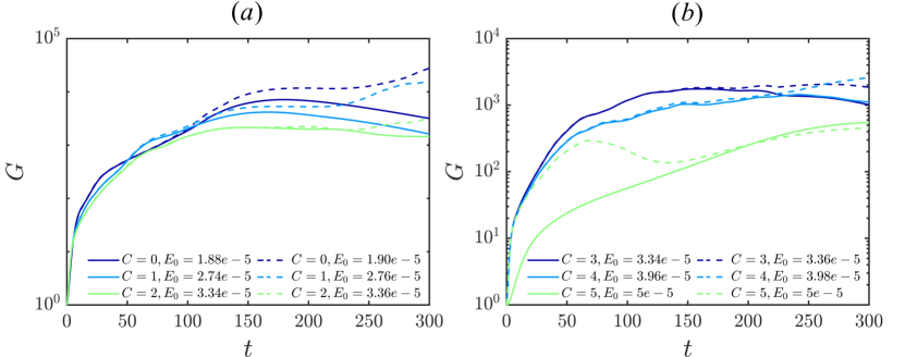
Figure 10: The energy growth of NLOP at $(a)$$C=0-2$ and $(b)$ $C=3-5$. In $(b)$ the solid green line represents the NLOP formed by the unstable eigenfunction, the dash green line refers to the NLOP as the same type one with $C<5$.

The structures of minimal seeds at $C=0,2$ are shown in figure 11. They are essentially similar, localised both in azithmuthal and streamwise direction, consistent with previous reports (Pringle & Kerswell, 2010; Pringle et al., 2012). But compared with isothermal pipe flow $C=0$, the minimal seed at $C=2$ is more localised, and thinner structure can be observed in radial direction, see figure 11($c,d$). A thinner minimal seed was reported by Marensi et al. (2019) for a (prescribed) flattened base velocity profile. Here the flattened profile is due to the buoyancy. The effective interval of the lift-up mechanism is narrowed and closer to the wall, consequently the optimal rolls and streamwise perturbation approaches the wall and gradually becomes thinner. Structures of the NLOP at $C=3,4$ (not shown) are similar to figure 11($d$), but thinner and closer to the wall.

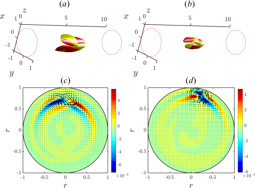
Figure 11: The iso-surface of optimal streamwise velocity perturbation and contour of that in cross section $Z=5$ for ($a,c$) $C=0,E_{0}=1.9e-05$ and ($b,d$) $C=2,E_{0}=3.36e-05$ at $Re=3000$, red/yellow are $30\%$ of the min/max streamwise velocity in iso-surface. The arrow represents the optimal cross-stream components, the largest arrow has magnitude $1.55e-04$ in $(a)$ and $2.39e-4$ in $(b)$.

The optimal perturbation at $C=5$ formed by unstable eigenfunction is shown in figure 12$(a)$, accompanied by the same branch of optimal perturbation at $C=4$ in figure 12$(b)$, found by using a longer target time $T_{opt}=400$ (to enable slower linear growth to compete with the NLOP). This type of optimal perturbation is almost unchanged at small $E_{0}$, suggesting linearity. Its structures are initially also close to the wall, but after an initial transient growth, they are rolled up near the centre of the pipe, approaching the unstable eigenfunctions. The exponential growth rate is in good agreement with the linear stability analysis.

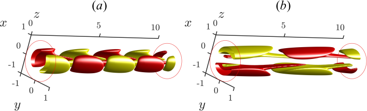
Figure 12: The iso-surface of streamwise velocity of optimal perturbation for ($a$)$C=4$ ($T_{opt}=400$ ) and ($b$) $C=5$ at $Re=3000$, red/yellow are $30\%$ of the min/max value in iso-surface.

For the interesting case at $C=6$, a NLOP with structure similar to those found at $C<5$ was not found with the previous parameters. By reducing the initial energy and extending the target time substantially ($E_{0}\sim O(10e-7)$, $T_{opt}=1000$), we finally located a new type of NLOP. Energy growth as a function of time is shown in figure 13. Optimals at all energies experience a period of energy growth at the beginning. Then, for a small initial energy $E_{0}=1e-8$, it exponentially decays. At larger initial energy, below the critical energy, the energy grows a little but finally still decays, albeit slowly. For this reason the long optimisation time $T_{opt}=1000$ was required. At slightly larger $E_{0}$ still, the critical energy jump is observed, see figure 13($b$).

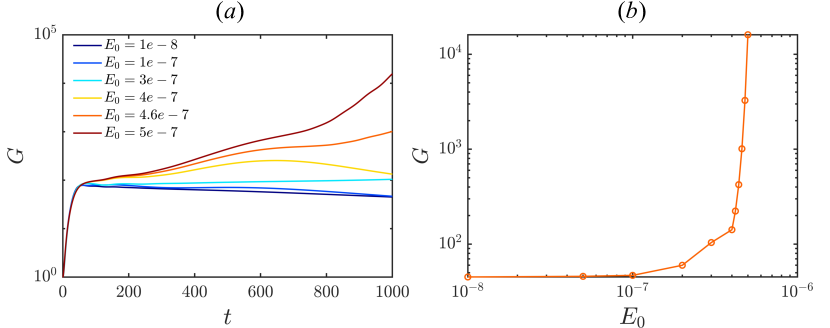
Figure 13: The optimal energy growth changes with ($a$) time and ($b$) $E_{0}$ at $C=6,Re=3000,T_{opt}=1000$.

Isosurfaces of the optimals at different $E_{0}$ for $C=6$ are shown in figure 14. Unlike the NLOP at $C=0-4$, its structure is observed to change over the range of $E_{0}$ for which it beats the linear optimal. The linear optimal is shown in figure 14($a$), which is distributed regularly in the streamwise direction, but with a great difference with linear optimal in isothermal case. For a larger $E_{0}$, as shown in 14($b,c$), the NLOP has a more spiral structure. As the initial energy increases further, streamwise localisation is observed in 14($d$), which is the minimal seed which eventually triggers turbulence. Its cross-section shows two pairs of streamwise vortices in the centre of the pipe, see figure 15, but with a very small magnitude compared with streamwise velocity.

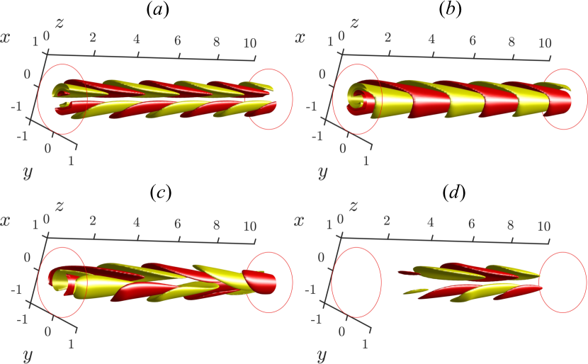
Figure 14: The streamwise perturbation iso-surface of the NLOP with different initial energy at $C=6$,($a$)$E_{0}=1e-8$,($b$)$E_{0}=1e-7$,($c$)$E_{0}=3e-7$,($d$)$E_{0}=4e-7$, red/yellow are 30$\%$ of the min/max value.

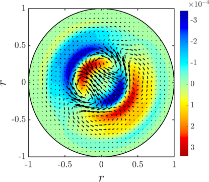
Figure 15: The cross section at $Z=5$ of NLOP with $E_{0}=4e-7$, the contour is colored by streamwise perturbation, the arrows represent the cross-stream components,the largest arrow has magnitude $4.44e-07$.

3.4 Transition to convective turbulence

The transition to shear turbulence via the NLOP has been widely researched in isothermal flow (Pringle & Kerswell, 2010; Pringle et al., 2012; Marensi et al., 2019), therefore we focus on the transition to convective turbulence here. In figure 16($a$), transition at $C=4$ and $\Rey=3000$ is compared for several initial conditions — shear-turbulence, the minimal seed, and unstable eigenfunctions. $E_{3d}$ is the energy of the streamwise-dependent component of the flow (modes $k\neq 0$ in the Fourier expansion). For the minimal seed, $E_{3d}$ increases substantially at first, reaching a shear-turbulent state. It then decays to the convective turbulence state. This implies that shear turbulence can still be triggered in the buoyancy regime, but it is not sustained. Starting from an arbitrary shear turbulence field, there is an immediate decay at first, then $E_{3d}$ grows exponentially towards convective turbulence. Interestingly, starting from the unstable eigenfunctions, the dynamics approaches a travelling wave solution (mode 2) or relative periodic solutions (mode 1 and mode 3). These states can be approached for a long time, suggesting that the travelling wave and relative periodic orbit solutions are only weakly unstable. An equilibrium state and periodic motion have also been reported in early research (Kemeny & Somers, 1962; Scheele & Hanratty, 1962; Yao, 1987), but at low Reynolds number $(Re<2000)$

At $C=5$, the unstable eigenfunction does not lead to a travelling wave or periodic solution, and instead transitions to convective turbulence directly, as shown in figure 16($b$). This may be due to the enhanced instability of these equilibrium solutions at larger $C$. The minimal seed at $C=5$ also triggers the convective turbulence directly, or at least, there is no period of decay after the initial growth, which would indicate a distinct switch from a shear-driven to convection-driven state. Meanwhile, starting from shear turbulence, there is a clear initial decay, followed by exponential growth at a rate which matches that starting from the eigenfunction.

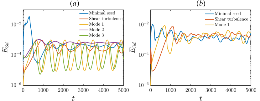
Figure 16: $E_{3d}$ (energy of streamwise-dependent component of the flow) for different initial conditions at ($a$) $C=4$ and ($b$) $C=5$ at $Re=3000$. There are three unstable modes at $C=4$: mode 1($m=1,k=2$),mode 2($m=1,k=1$), mode 3($m=1,k=3$). There is only one unstable mode at $C=5$ ($m=1,k=1$).

The transition process at $C=6$, where the laminar state is linearly stable, is quite different. The transition starting from the NLOP at $C=6$ with different $E_{0}$ are shown in figure 17. Compared with the transition via the NLOP in the isothermal case (Pringle et al., 2012), the process of transition is much slower: the earliest time turbulence is seen at approximately $t=1000$ in the figure, and hence the large target time $T=1000$ required. The edge state (Duguet et al., 2008), here to the convective turbulent state, appears to be less unstable than that for the shear turbulent state, as intermediate energies before transition can be achieved for long times with little refinement of the initial energy. Some typical coherent structures that appear in the process of transition are presented in figure 18, starting from slightly different initial energies(left/right). Initially the contours of minimal seed are tightly layered and forward-facing, but because the base profile is M-shaped, the structures are inclined into the shear, see figure 14$(d)$. This is opposite to that for the iso-thermal minimal seed, where the layers are backward-facing and inclined into the shear (Pringle et al., 2012). Therefore, between $t=0$ and $t=T_{1}$ there is a great energy growth in a very short time through the Orr mechanism (Orr, 1907; Pringle et al., 2012). Then it evolves to a simpler organised state at $t=T_{2}$, figure 18$(\it b)$, and both flows still look similar. At $t=T_{3}$ $(\it c)$, the structure on the right is more elongated, it looks similar to the travelling wave solution of figure19$(a)$, then it evolves into the convective state at $T_{4}$(d,right). On the left, the solution decays. At $t=T_{4}$(d,left), the NLOP for $E_{0}=4e-7$ gradually decays exponentially, but with a very small decay rate. For the NLOP of $E_{0}=4.2e-7$, a relatively rapid increase of energy is observed, and a similar final growth stage is observed for the NLOPs of larger initial energies, see figure 17. Overall, the transition process of minimal seed is complex and long compared to that for the minimal seed for transition to shear-turbulence.

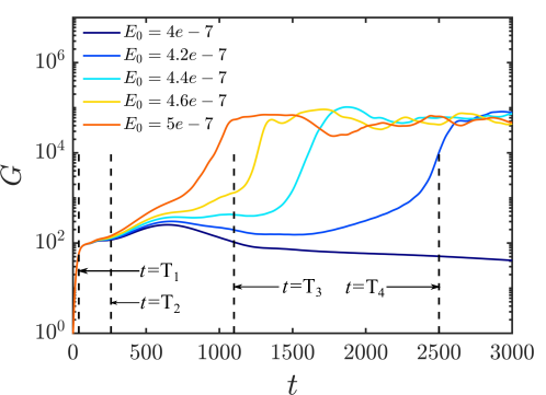
Figure 17: The energy changing in a longer time for the NLOP obtained in different $E_{0}$ for the case of $C=6,Re=3000$. The cases $E_{0}=4e-7,4.6e-7,5e-7$ were also shown in figure 13 only up to a shorter time.

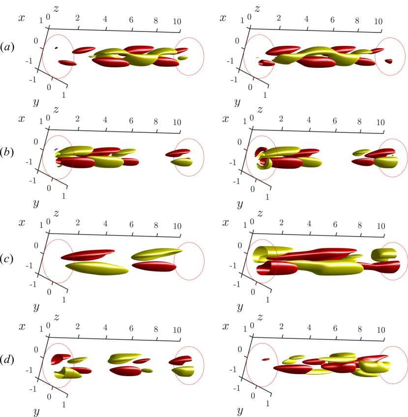
Figure 18: The iso-surface of streamwise velocity at ($a$) $t=T_{1}$ , ($b$) $t=T_{2}$, ($c$) $t=T_{3}$, ($d$)$t=T_{4}$, the figures in the left hand are sampled from the case of $E_{0}=4e-7,C=6,Re=3000$, the figures in the right hand are sampled from the case of $E_{0}=4.2e-7,C=6,Re=3000$, time is marked in figure 17,red/yellow are 30$\%$ of the min/max value.

In recent years, a series of invariant solutions of Navier-Stokes equations are found in pipe flow(Wedin & Kerswell, 2004; Hof et al., 2004; Eckhardt et al., 2007) and other shear flow(Nagata, 1990; Toh & Itano, 2003; Reetz et al., 2019). These invariant solutions significantly rich the understanding to the transition and maintenance of turbulence. Especially, the periodic solution (Toh & Itano, 2003) extracted in channel flow successfully reproduces the self-sustaining process of shear turbulence(Hamilton et al., 1995), which perfects the mechanism of maintenance of shear turbulence mathematically. Although, these solutions are unstable, the dimensions of their unstable manifolds in phase space are typically low(Kawahara, 2005; Kerswell & Tutty, 2007). It is not expected to observe them in the real turbulence, a generic turbulent state could approach them and spend a substantial fraction of its lifetime in their neighborhood(Kawahara et al., 2012).

In figure 16, the dynamics is obviously wandering around a travelling wave solution and periodic solutions. We therefore use states from the trajectory as an initial guess for the Jacobian-free Newton–Krylov (JFNK) method (Willis, 2017). The algorithm converged very quickly to a travelling wave solution and a periodic solution. The travelling wave solution is plotted in figure 19, which has a wave speed $c=0.6783$. The wavy high-speed streak in the centre of pipe, is formed by the merging of positive velocity motion in the nonlinear growth process, and is similar to the streak formed in the relative periodic orbits, see figure21$(a,b)$. Streamwise vorticity is localised in streamwise direction, located at the bends of the high-speed streak. Linear instability analysis of this travelling wave solution shows that it has only one unstable direction, implying that it is the edge state (Duguet et al., 2008). The eigenvalue of unstable eigenfunction is small $(2.56e-4)$, so that excessive refinement of the initial energy is not required to stay close to the state for some time.

The periodic solutions approached from the first and third unstable eigenfunctions, marked $PO_{1}$ and $PO_{2}$ respectively, have long periods, $T_{1}=724.4$ and $T_{2}=623.72$. They are similar, only with a different dominant axial wave number ($k=2$ for $PO_{1}$ and $k=3$ for $PO_{2}$). We here pay attention to the periodic solution triggered by the first unstable mode. The energy of three components is presented in figure 20$(a)$, energy of the rolls, $E_{roll}=E(u_{r})+E(u_{\theta})$, energy of the streaks, $E_{streak}=E(u_{z})_{k=0}$, and energy of waves, $E_{waves}=E(u_{z})_{k\neq 0}$, where the subscripts $k=0$ and $k\neq 0$ indicate streamwise independent and dependent components extracted via the Fourier decomposition. As a single streak forms at the centre of the pipe, we have not split azimuthal dependence through $m$. For the well-known periodic solution found in channel flow by Hamilton et al. (1995), the peak of the roll energy almost corresponds to the valley of the streak energy. For the current periodic solution, these energies are more offset. Contours of streamwise perturbaton velocity $u_{z}$ at $t=500,700,900,1100$ are shown in figure 21, which reveals the changing of structure over one period. At $t=500$, the streak energy is at its lowest, and the velocity field resembles the unstable eigenfunction, only with a weak break of shift and reflect symmetry. Then, by $t=700$ the unstable eigenfunction has grown until regions of positive velocity have merged, forming a high-speed streak in the centre of the pipe. In the presence of the streak, the roll perturbations decay, $t=900$, then return once the streak has weakened at $t=1100$. Therefore, three typical stages are observed in the periodic solution, i.e. growth of the eigenfunction, formation of the streak and decay of the streak. These processes can be understood from the changes of the mean velocity profile, seen in figure 20$(b)$. At first, when the perturbation is weak, the velocity profile is close to the laminar solution $(t=500)$. The linear instability takes charge of the dynamics, and the unstable eigenfunction grows at that stage. Then, when the perturbation excites a sufficiently strong streak near the axis, the velocity profile is more flattened $(t=700,900)$ and the linear instability is suppressed, causing the perturbation to decay. Once the perturbation decays to certain level, the velocity profile becomes unstable again $(t=1100)$ and the process repeats, the detailed periodic process is shown in the supplementary movies 1.

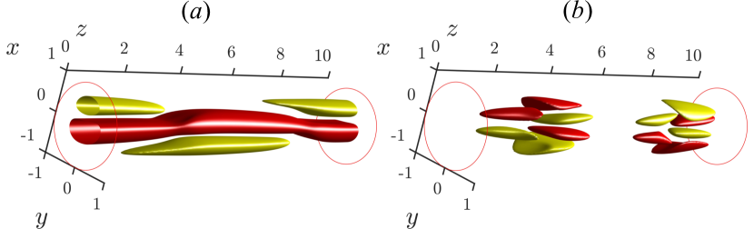
Figure 19: The travelling wave solution found in the flow at $C=4,Re=3000$, $(a)$ the isosurface of streamwise perturbation, $(b)$ the isosurface of streamwise vorticity,red/yellow are 30$\%$ of the min/max value.

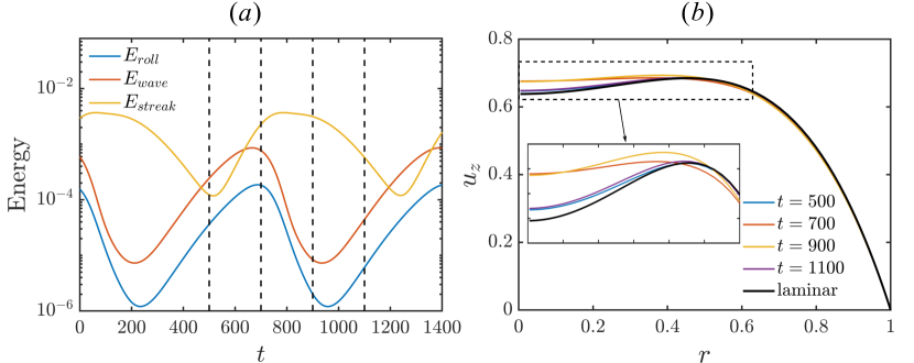
Figure 20: $(a)$ Time evolution of the energy of periodic solution $PO_{1}$ at $C=4,Re=3000$, here $E_{roll}=E(u_{r})+E(u_{\theta})$, $E_{wave}=E(u_{z})_{k\neq 0}$, $E_{streak}=E(u_{z})_{k=0}$, $(b)$ the turbulent mean velocity profile at different time

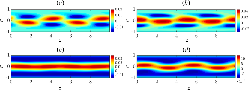
Figure 21: The contour of periodic solution $PO_{1}$ at $(a)t=500$,$(b)t=700$,$(c)t=900$,$(d)t=1100$, colored by streamwise velocity disturbance $u$.

Similar phenomena occurs in the convective state at $C=4$, but in this case, the laminar flow is unstable to multiple modes. The contours of transient turbulence show that the flow neither comes to a periodic state or travelling wave state, figure 22. But the convective turbulence still presents the three typical processes, i.e, the growth of unstable modes (figure 22$(a)$), the formation of high speed streak (figure 22$(b)$), decay of the streak and reappearance of the unstable modes (figure 22$(c,d)$). The scales of the observed modes are in good agreement with the first unstable mode and third unstable mode, which means the flow may be wandering around the two periodic solutions. The scale of the travelling wave (unstable edge solution) is hardly observed.

The periodic solutions become more unstable at larger $C$, thus the flow is more chaotic. However, the typical process can be still observed, as in figure 23, which shows two transient flow states taken from the flow at $C=5$. Figure 23$(b)$ shows typical growth of an unstable mode, upon a mean velocity profile shown in figure 23$(a)$. It is observed that the profile is close to the laminar profile, but does not go so close as the case at $C=4$ shown in figure 20$(b)$, as the laminar solution is more unstable. The flow state in figure 23$(c)$ is the high speed streak formed by the growth of unstable mode, whose profile is almost flattened and loses the linear instability. These typical flow states can be often observed at $C=5$, and can even be observed at $C=10$, although less clearly. Therefore, it appears that the convective turbulence is self-sustained by these typical stages, i.e. the growth of unstable modes, the formation of streak and the decay of streaks.

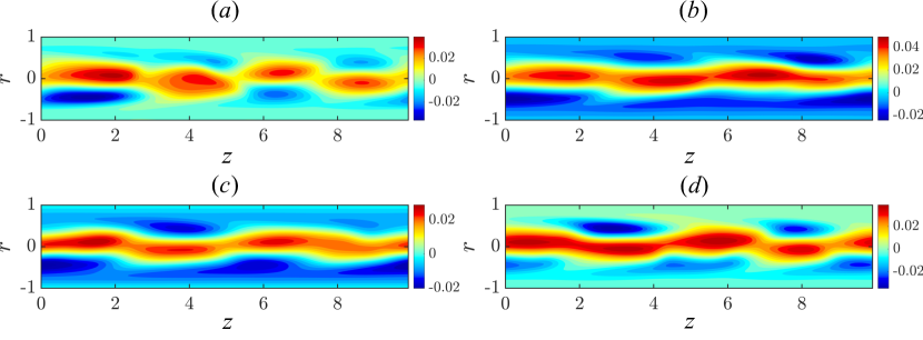
Figure 22: The contour of transient convective turbulence at $(a)t=2500$,$(b)t=2750$,$(c)t=3000$,$(d)t=3250$, picked form figure 16 when the turbulence is triggered by shear turbulence at $C=4$, the contour is colored by streamwise velocity disturbance $u$.

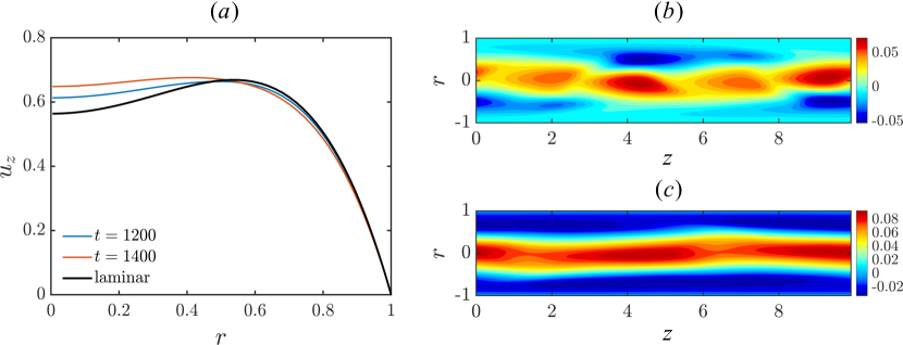
Figure 23: $(a)$ The turbulent mean profiles of the flow at $(b)$ and $(c)$. The contour of transient convective turbulence at $(b)t=1200$,$(c)t=1400$, picked form figure 16 when the turbulence is triggered by shear turbulence at $C=5$, the contour is colored by velocity disturbance $u$.

4 Conclusion

In this study, a new DNS model that includes time-dependent heat flux and background temperature gradient is established. The results show good consistency with experiment and a little improvement over the model of Marensi et al. (2021), which also had time-dependent heat flux, but a spatially-uniform heat sink term. The simulations at different buoyancy condition confirm three typical flow states, i.e. shear turbulence, laminarisation and convective turbulence. The distribution of these states in the parameter space is consistent with the calculations of Marensi et al. (2021). Detailed insight to the convective turbulence found it lacks near wall rolls to enhance the mixing of fluid near the wall and centre, the heat transfer is thus damaged seriously. The linear stability analysis further verifies that the convective turbulence is driven by linear instability (Yao, 1987; Su & Chung, 2000; Khandelwal & Bera, 2015; Marensi et al., 2021). The structures of unstable eigenfunctions are found to be mainly concentrated on the centre of pipe, which explains the similar flow characteristics observed in the transient convective turbulence.

Nonlinear non-modal stability analysis is extended to the heated pipe case to determine the effects of buoyancy on the minimal seed. It is found that the structure of the minimal seed become thinner and the rolls move nearer the wall, and the critical energy for transition increases as the buoyancy is gradually enhanced. The maximum energy growth occurs earlier and is greatly reduced. Importantly, this suggests that strategies for exciting shear turbulence, in order to encourage greater heat flux, do not straightforwardly carry over from the isothermal to the heated pipe case. The branch of NLOP that triggers turbulence in isothermal flow, could not be tracked beyond $C=5$, due to the combined reduction in growth and enhancement of linear instability. Instead, a new type of NLOP arises for a longer target time and for a small initial energy. The new NLOP changes structure as the initial energy is increased, localising in the streamwise direction for the minimal seed. It is concentrated towards the centre of pipe, triggering convective turbulence directly, but over a long time period.

The transitions towards convective turbulence at $C=4,5,6$ triggered by the NLOP were compared with transition via the unstable eigenfunctions. At $C=4$, it is found that starting from the unstable eigenfunctions leads to a travelling wave solution or periodic solutions, while the minimal seed first triggers shear turbulence, then the shear turbulence decays to convective turbulence. At $C=5$, both unstable eigenfunctions and the minimal seed trigger convective turbulence directly. At $C=6$, the transition starting from the new NLOP is much slower, compared with that which triggers shear turbulence. The edge state to the convective turbulence appears to be less unstable than that for shear turbulence, and intermediate energies before transition can be achieved for longer time with little refinement of the initial energy. ‘Exact’ solutions for the travelling wave solution and periodic solution were calculated using Jacobian-free Newton–Krylov (JFNK) method, and their stability. The traveling wave solution only has one unstable dimension, confirmed as edge state.

The periodic solution is found to distill three typical processes, i.e. the growth of an unstable eigenfunction, the formation of streak and decay of the streak. Analysis of the mean velocity profile showed that the periodic process is caused by the appearance and suppression of linear instability of the mean velocity profile. This is fundamentally different from the self-sustaining process of isothermal shear flow, which occurs in the absence of linear instability of the mean flow. The transient convective turbulence at $C=4$ shows the flow is still dominated by the three typical processes, but consists of the scales of two periodic solutions, suggesting the flow may be wandering between these two periodic solutions in phase space. A similar phenomena can be still often observed at $C=5$, and can be recognised even up to $C=10$.

[Supplementary movies]Supplementary movies are available

[Acknowledgements] This work used the Cirrus UK National Tier-2 HPC Service at EPCC (http://www.cirrus.ac.uk) funded by the University of Edinburgh and EPSRC (EP/P020267/1).

[Funding] S.C. acknowledges the funding from Sheffield–China Scholarships Council PhD Scholarship Programme (CSC no. 202106260029).

[Declaration of interests]The authors report no conflict of interest.

[Author ORCIDs] Shijun Chu, https://orcid.org/0000-0002-3037-6370; Ashley P. Willis, https://orcid.org/0000-0002-2693-2952; Elena Marensi, https://orcid.org/0000-0001-7173-4923.

References

- Ackerman (1970) Ackerman, JW 1970 Pseudoboiling heat transfer to supercritical pressure water in smooth and ribbed tubes .
- Avila et al. (2011) Avila, Kerstin, Moxey, David, De Lozar, Alberto, Avila, Marc, Barkley, Dwight & Hof, Björn 2011 The onset of turbulence in pipe flow. Science 333 (6039), 192–196.
- Avila et al. (2023) Avila, Marc, Barkley, Dwight & Hof, Björn 2023 Transition to turbulence in pipe flow. Annual Review of Fluid Mechanics 55, 575–602.
- Bae et al. (2005) Bae, Joong Hun, Yoo, Jung Yul & Choi, Haecheon 2005 Direct numerical simulation of turbulent supercritical flows with heat transfer. Physics of fluids 17 (10).
- Bae et al. (2006) Bae, Joong Hun, Yoo, Jung Yul, Choi, Haecheon & McEligot, Donald M 2006 Effects of large density variation on strongly heated internal air flows. Physics of Fluids 18 (7).
- Celataa et al. (1998) Celataa, Gian Piero, Dannibale, Francesco, Chiaradia, Andrea & Cumo, Maurizio 1998 Upflow turbulent mixed convection heat transfer in vertical pipes. International journal of heat and mass transfer 41 (24), 4037–4054.
- Chen & Chung (1996) Chen, Yen-Cho & Chung, JN 1996 The linear stability of mixed convection in a vertical channel flow. Journal of Fluid Mechanics 325, 29–51.
- Chen & Chung (2002) Chen, Yen-Cho & Chung, JN 2002 A direct numerical simulation of k-and h-type flow transition in a heated vertical channel. Physics of Fluids 14 (9), 3327–3346.
- Cherubini & De Palma (2013) Cherubini, Stefania & De Palma, Pietro 2013 Nonlinear optimal perturbations in a couette flow: bursting and transition. Journal of Fluid Mechanics 716, 251–279.
- Cherubini et al. (2011) Cherubini, Stefania, De Palma, Pietro, Robinet, J-C & Bottaro, Alessandro 2011 The minimal seed of turbulent transition in the boundary layer. Journal of Fluid Mechanics 689, 221–253.
- Chu et al. (2024) Chu, Shijun, Willis, Ashley P. & Marensi, Elena 2024 Linear and nonlinear optimisation for laminarisation in pipe flow. In preparation.
- Chu et al. (2016) Chu, Xu, Laurien, Eckart & McEligot, Donald M 2016 Direct numerical simulation of strongly heated air flow in a vertical pipe. International Journal of Heat and Mass Transfer 101, 1163–1176.
- Duguet et al. (2008) Duguet, Yohann, Willis, Ashley P & Kerswell, Rich R 2008 Transition in pipe flow: the saddle structure on the boundary of turbulence. Journal of Fluid Mechanics 613, 255–274.
- Eckhardt et al. (2007) Eckhardt, Bruno, Schneider, Tobias M, Hof, Bjorn & Westerweel, Jerry 2007 Turbulence transition in pipe flow. Annu. Rev. Fluid Mech. 39, 447–468.
- Guo et al. (2007) Guo, Zeng-Yuan, Zhu, Hong-Ye & Liang, Xin-Gang 2007 Entransy—a physical quantity describing heat transfer ability. International Journal of Heat and Mass Transfer 50 (13-14), 2545–2556.
- Hall & Jackson (1969) Hall, William Bateman & Jackson, JD 1969 Laminarization of a turbulent pipe flow by buoyancy forces. In Mechanical Engineering, , vol. 91, p. 66. ASME-AMER SOC MECHANICAL ENG 345 E 47TH ST, NEW YORK, NY 10017.
- Hamilton et al. (1995) Hamilton, James M, Kim, John & Waleffe, Fabian 1995 Regeneration mechanisms of near-wall turbulence structures. Journal of Fluid Mechanics 287, 317–348.
- Hanratty et al. (1958) Hanratty, Thomas J, Rosen, Edward M & Kabel, Robert L 1958 Effect of heat transfer on flow field at low reynolds numbers in vertical tubes. Industrial & Engineering Chemistry 50 (5), 815–820.
- He et al. (2021) He, J, Tian, R, Jiang, PX & He, S 2021 Turbulence in a heated pipe at supercritical pressure. Journal of Fluid Mechanics 920, A45.
- He et al. (2016) He, S, He, K & Seddighi, M 2016 Laminarisation of flow at low reynolds number due to streamwise body force. Journal of Fluid mechanics 809, 31–71.
- Herbert (1983) Herbert, Thorwald 1983 Secondary instability of plane channel flow to subharmonic three-dimensional disturbances. The Physics of Fluids 26 (4), 871–874.
- Hof et al. (2010) Hof, Björn, De Lozar, Alberto, Avila, Marc, Tu, Xiaoyun & Schneider, Tobias M 2010 Eliminating turbulence in spatially intermittent flows. science 327 (5972), 1491–1494.
- Hof et al. (2004) Hof, Bjorn, Van Doorne, Casimir WH, Westerweel, Jerry, Nieuwstadt, Frans TM, Faisst, Holger, Eckhardt, Bruno, Wedin, Hakan, Kerswell, Richard R & Waleffe, Fabian 2004 Experimental observation of nonlinear traveling waves in turbulent pipe flow. Science 305 (5690), 1594–1598.
- Jackson (2013) Jackson, JD 2013 Fluid flow and convective heat transfer to fluids at supercritical pressure. Nuclear Engineering and Design 264, 24–40.
- Jackson & Li (2002) Jackson, JD & Li, J 2002 Influences of buoyancy and thermal boundary conditions on heat transfer with naturally-induced flow .
- Kawahara (2005) Kawahara, Genta 2005 Laminarization of minimal plane couette flow: going beyond the basin of attraction of turbulence. Physics of Fluids 17 (4).
- Kawahara et al. (2012) Kawahara, Genta, Uhlmann, Markus & Van Veen, Lennaert 2012 The significance of simple invariant solutions in turbulent flows. Annual Review of Fluid Mechanics 44, 203–225.
- Kemeny & Somers (1962) Kemeny, GA & Somers, EV 1962 Combined free and forced-convective flow in vertical circular tubes—experiments with water and oil .
- Kerswell & Tutty (2007) Kerswell, Rich R & Tutty, Owen R 2007 Recurrence of travelling waves in transitional pipe flow. Journal of Fluid Mechanics 584, 69–102.
- Khandelwal & Bera (2015) Khandelwal, Manish K & Bera, P 2015 Weakly nonlinear stability analysis of non-isothermal poiseuille flow in a vertical channel. Physics of Fluids 27 (6).
- Klebanoff et al. (1962) Klebanoff, Philip S, Tidstrom, KD & Sargent, LM 1962 The three-dimensional nature of boundary-layer instability. Journal of Fluid Mechanics 12 (1), 1–34.
- Kühnen et al. (2018) Kühnen, Jakob, Song, Baofang, Scarselli, Davide, Budanur, Nazmi Burak, Riedl, Michael, Willis, Ashley P, Avila, Marc & Hof, Björn 2018 Destabilizing turbulence in pipe flow. Nature Physics 14 (4), 386–390.
- Lellep et al. (2022) Lellep, Martin, Prexl, Jonathan, Eckhardt, Bruno & Linkmann, Moritz 2022 Interpreted machine learning in fluid dynamics: explaining relaminarisation events in wall-bounded shear flows. Journal of Fluid Mechanics 942, A2.
- Marensi et al. (2021) Marensi, Elena, He, Shuisheng & Willis, Ashley P 2021 Suppression of turbulence and travelling waves in a vertical heated pipe. Journal of Fluid Mechanics 919, A17.
- Marensi et al. (2019) Marensi, Elena, Willis, Ashley P & Kerswell, Rich R 2019 Stabilisation and drag reduction of pipe flows by flattening the base profile. Journal of Fluid Mechanics 863, 850–875.
- McEligot et al. (1970) McEligot, DM, Coon, CW & Perkins, HC 1970 Relaminarization in tubes. International Journal of Heat and Mass Transfer 13 (2), 431–433.
- Motoki et al. (2018) Motoki, Shingo, Kawahara, Genta & Shimizu, Masaki 2018 Optimal heat transfer enhancement in plane couette flow. Journal of Fluid Mechanics 835, 1157–1198.
- Nagata (1990) Nagata, Masato 1990 Three-dimensional finite-amplitude solutions in plane couette flow: bifurcation from infinity. Journal of Fluid Mechanics 217, 519–527.
- Orr (1907) Orr, William M’F 1907 The stability or instability of the steady motions of a perfect liquid and of a viscous liquid. part ii: A viscous liquid. In Proceedings of the Royal Irish Academy. Section A: Mathematical and Physical Sciences, , vol. 27, pp. 69–138. JSTOR.
- Poskas et al. (2012) Poskas, P, Poskas, R & Gediminskas, A 2012 Numerical investigation of the opposing mixed convection in an inclined flat channel using turbulence transition models. In Journal of Physics: Conference Series, , vol. 395, p. 012098. IOP Publishing.
- Pringle & Kerswell (2010) Pringle, Chris CT & Kerswell, Rich R 2010 Using nonlinear transient growth to construct the minimal seed for shear flow turbulence. Physical review letters 105 (15), 154502.
- Pringle et al. (2012) Pringle, Chris CT, Willis, Ashley P & Kerswell, Rich R 2012 Minimal seeds for shear flow turbulence: using nonlinear transient growth to touch the edge of chaos. Journal of Fluid Mechanics 702, 415–443.
- Reetz et al. (2019) Reetz, Florian, Kreilos, Tobias & Schneider, Tobias M 2019 Exact invariant solution reveals the origin of self-organized oblique turbulent-laminar stripes. Nature communications 10 (1), 2277.
- Rogers & Yao (1993) Rogers, BB & Yao, LS 1993 Finite-amplitude instability of mixed-convection in a heated vertical pipe. International journal of heat and mass transfer 36 (9), 2305–2315.
- Scheele & Hanratty (1962) Scheele, George F & Hanratty, Thomas J 1962 Effect of natural convection on stability of flow in a vertical pipe. Journal of Fluid Mechanics 14 (2), 244–256.
- Scheele et al. (1960) Scheele, George F, Rosen, Edward M & Hanratty, Thomas J 1960 Effect of natural convection on transition to turbulence in vertical pipes. The Canadian Journal of Chemical Engineering 38 (3), 67–73.
- Su & Chung (2000) Su, Yi-Chung & Chung, Jacob N 2000 Linear stability analysis of mixed-convection flow in a vertical pipe. Journal of Fluid Mechanics 422, 141–166.
- Toh & Itano (2003) Toh, Sadayoshi & Itano, Tomoaki 2003 A periodic-like solution in channel flow. Journal of Fluid Mechanics 481, 67–76.
- Turner & Turner (1979) Turner, John Stewart & Turner, John Stewart 1979 Buoyancy effects in fluids. Cambridge university press.
- Wang et al. (2011) Wang, Jianguo, Li, Huixiong, Yu, Shuiqing & Chen, Tingkuan 2011 Investigation on the characteristics and mechanisms of unusual heat transfer of supercritical pressure water in vertically-upward tubes. International Journal of Heat and Mass Transfer 54 (9-10), 1950–1958.
- Wedin & Kerswell (2004) Wedin, Hakan & Kerswell, Rich R 2004 Exact coherent structures in pipe flow: travelling wave solutions. Journal of Fluid Mechanics 508, 333–371.
- Wibisono et al. (2015) Wibisono, Andhika Feri, Addad, Yacine & Lee, Jeong Ik 2015 Numerical investigation on water deteriorated turbulent heat transfer regime in vertical upward heated flow in circular tube. International Journal of Heat and Mass Transfer 83, 173–186.
- Willis (2017) Willis, Ashley P 2017 The openpipeflow navier–stokes solver. SoftwareX 6, 124–127.
- Yao (1987) Yao, LS 1987 Is a fully-developed and non-isothermal flow possible in a vertical pipe? International journal of heat and mass transfer 30 (4), 707–716.
- Yoo (2013) Yoo, Jung Yul 2013 The turbulent flows of supercritical fluids with heat transfer. Annual review of fluid mechanics 45, 495–525.
- You et al. (2003) You, Jongwoo, Yoo, Jung Y & Choi, Haecheon 2003 Direct numerical simulation of heated vertical air flows in fully developed turbulent mixed convection. International Journal of Heat and Mass Transfer 46 (9), 1613–1627.
- Zhang et al. (2020) Zhang, Shijie, Xu, Xiaoxiao, Liu, Chao & Dang, Chaobin 2020 A review on application and heat transfer enhancement of supercritical co2 in low-grade heat conversion. Applied Energy 269, 114962.
- Zhao et al. (2018) Zhao, Pinghui, Zhu, Jiayin, Ge, Zhihao, Liu, Jiaming & Li, Yuanjie 2018 Direct numerical simulation of turbulent mixed convection of lbe in heated upward pipe flows. International Journal of Heat and Mass Transfer 126, 1275–1288.