[1]\fnmGopal \surAgarwal \equalcontThese authors contributed equally to this work.
[2]\fnmJorge-Humberto \surUrrea-Quintero \equalcontThese authors contributed equally to this work.
[2]\fnmHenning \surWessels
[1]\fnmThomas \surWick
1]\orgnameLeibniz University Hannover, \orgdivifam - Institut für Angewandte Mathematik, \orgaddress\streetWelfengarten 1, \cityHannover, \postcode30167, \stateLower Saxony, \countryGermany
2]\orgnameTechnische Universtität Braunschweig, \orgdiviRMB - Institute for Computational Modeling in Civil Engineering, \orgaddress\streetPockelsstr. 3, \cityBraunschweig, \postcode38106, \stateLower Saxony, \countryGermany
3]\orgnameLeibniz University Hannover, \orgdivCluster of Excellence PhoenixD (Photonics, Optics, and Engineering - Innovation Across Disciplines), \orgaddress\streetWelfengarten 1, \cityHannover, \postcode30167, \stateLower Saxony, \countryGermany
Model order reduction for transient coupled diffusion-deformation of hydrogels
Abstract
This study introduces a reduced-order model (ROM) for analyzing the transient diffusion-deformation of hydrogels. The full-order model (FOM) describing hydrogel transient behavior consists of a coupled system of partial differential equations in which chemical potential and displacements are coupled. This system is formulated in a monolithic fashion and solved using the Finite Element Method (FEM). The ROM employs proper orthogonal decomposition as a model order reduction approach. We test the ROM performance through benchmark tests on hydrogel swelling behavior and a case study simulating co-axial printing. Finally, we embed the ROM into an optimization problem to identify the model material parameters of the coupled problem using full-field data. We verify that the ROM can predict hydrogels’ diffusion-deformation evolution and material properties, significantly reducing computation time compared to the FOM. The results demonstrate the ROM’s accuracy and computational efficiency. This work paths the way towards advanced practical applications of ROMs, e.g., in the context of feedback error control in hydrogel 3D printing.
keywords:
hydrogels modeling, model-order reduction, proper orthogonal decomposition, model material parameters identification, coupled problems, finite elements, FEniCS, RBniCS1 Introduction
The emergence of bioprinting technologies has opened new frontiers in engineering functional materials for biomedical applications. Hydrogels, known for their biocompatibility, high water content, and adaptable mechanical properties, are at the forefront of this innovation [43]. The fabrication of hydrogels has been supported by the integration of quantitative experimental techniques with computational models describing the material and mechanical properties of the fabricated hydrogel. A comprehensive review of available experimental methods to investigate hydrogel properties can be found in [10], along with an overview of some common mathematical modeling approaches describing hydrogels’ mechanics and transport properties. A recent review of the theories capturing hydrogel’s diffusion-deformation coupled mechanisms in the large deformation setting can be found in [39].
Diffusion-deformation models for hydrogels combine continuum mechanics and thermodynamics with solvent diffusion physics through, e.g., the balance of mass and Fick’s law of diffusion [13, 8, 29], but lack an analytical solution in general [15, 39]. This requires numerical methods, such as the Finite Element Method (FEM), to approximate the model’s solution [2, 39]. Running such full-order model (FOM) finite element simulations becomes costly in many-query tasks such as model parameter identification, optimization, model-based 3D printing monitoring, or feedback printing error compensation technologies, in which several hundreds or thousands of similar runs are often necessary. This has prevented hydrogels modeling widespread adoption in design, optimization, process monitoring, or feedback error compensation.
Model-order reduction (MOR) offers a promising solution to the challenges posed by the computational burden of multiphysics models. By using a ROM, we can save on computation resources while still capturing the dominant behaviors of the system. This makes ROMs suitable for tasks such as material parameter identification [45], uncertainty quantification [36], process optimization, or feedback error compensation during printing [27, 38]. They can be tailored to specific regions of interest, ensuring accuracy where it is most crucial. By integrating ROMs, uncertainties in parameter spaces can also be more effectively managed [11]. ROMs can bridge the gap between the detailed insights provided by multiphysics models and the practical necessities of, e.g., model-guided hydrogels printing.
In the MOR literature, Proper Orthogonal Decomposition (POD) and its variants are particularly popular across multiple disciplines; see, e.g., [33] for a review of POD methods for MOR in a variety of research areas. For example, POD has been successfully applied in engineering, in the context of fluid mechanics [20, 3, 35], image processing [40], rotor dynamics [30, 32], for structural damage detection [17], and in the area of structural dynamics [24]. In addition, POD methods can be used to solve optimal control problems [34, 9, 4]. Moreover, the POD approach can be physically interpreted based on the concept of proper orthogonal modes (POMs) [24]. However, while the theory is solid for linear and some non-linear systems [6], applying ROMs to tasks such as hydrogels fabrication by printing is largely unexplored. In this work, we exploit the capabilities of POD to predict the transient diffusion-deformation of hydrogels in co-axial printing and its efficiency in tasks such as material parameter identification.
Different POD variants have been proposed in the literature. Global POD methods focus on the estimation of global POD coefficients [5, 6]. In contrast, local POD methods are based on snapshot clustering [37]. Adaptive POD methods have been developed to improve POD basis functions construction by choosing additional snapshot locations in an optimal way [26]. Incremental POD has also been proposed, allowing an adaptive enrichment of the POD basis in case of unforeseen changes in the solution behavior [18, 19]. Transient POD methods focus on snapshots of a transient process [31]. The so-called nested POD applies to time-dependent partial differential equations (PDEs) and allows for a two-step compression process, first in time and then in the parameters space [22, 23]. This approach has been shown to be particularly useful when the PDE requires many steps to be approximated. It reduces the memory storage requirements of the traditional POD and is the method of choice in the present study.
We consider a specialized theory for small deformations superposed on a previously homogeneously swollen gel as presented by [2]. This model is derived following rigorous thermodynamic concepts and can be considered the linearized version of the more general theory presented by [13] and [15]. This diffusion-deformation model was recently validated by [12] and showed good agreement with the experimental data. We implement a reduced-order model using POD, balancing computational efficiency with model fidelity. We discuss the ROM’s accuracy and evaluate the computation speed-up to assess its suitability for many-query scenarios in preparation for more challenging tasks such as bioprinting feedback error compensation.
The main contributions of the paper can be summarized as follows:
-
•
The application of POD as a ROM to efficiently capture the FOM dynamics describing the coupled hydrogel diffusion-deformation process.
-
•
The verification of the POD accuracy in a well-known benchmark example, free-swelling of a 2D square block, and a case study, co-axial printing, and speeding up computation comparison with respect to the FOM.
-
•
The evaluation of POD’s effectiveness for material parameter identification in hydrogel printing processes.
The paper is organized as follows: Section 2 summarizes the coupled diffusion-deformation theory of gels in the small deformation regime. Section 3 introduces the POD framework. Section 4 states the material parameter identification problem enabled by the reduced-order model. In section 5, several simulations are conducted and computationally analyzed. Concluding remarks are given in Section 6.
2 Small deformations theory for the diffusion-deformation of hydrogels
Diffusion-deformation theories of gels integrate fluid transport and solid mechanics principles to explain how gels swell or shrink due to fluid movement and how these processes influence their shape and mechanical properties [13, 8, 15, 39]. In a diffusion-deformation model of gels, the driving forces are fluid diffusion into or out of the gel and mechanical deformation due to external loads or internal stresses. The model should allow for predicting swelling or shrinking behaviors, stress distributions, and changes in mechanical properties over time. The primary outcomes of this model include the gel’s deformation patterns and mechanical responses under varying conditions. Essential parameters for model calibration encompass the diffusion coefficient, the gel matrix’s mechanical properties such as Young’s modulus and Poisson’s ratio, and fluid-gel interaction parameters such as Flory’s interaction parameter.
This section summarizes the theory describing the diffusion-deformation mechanisms in elastomeric gels that undergo small deformations under isothermal conditions. The model is derived as a special case of a more general theory of chemoelasticity [1, 2]. The coupled deformation-diffusion theory presented in this section is often employed in the small deformation analysis of previously swollen polymer gels [2, 12]. If very large deformations are present, a more suitable theory accounting for the hyperelastic deformation of the polymer network and describing the mixing of the solvent with the polymer network should be considered [13, 8, 15, 39].
As notation rules, we denote gradient and divergence . The time derivative of any field is denoted by . The operator refers to the trace of the second-order tensor . We denote the spatial dimension with , and in this section, we exclusively work with . Finally, let be the time interval with end time value and its closure.
2.1 Kinematics of the deformation
Consider a continuum homogeneous elastomeric body within the Euclidean space and its boundary . Here, denotes the displacement (Dirichlet) boundary, the traction (Neumann) boundary, and the fluid flux (Robin) boundary. The outward normal vector to the domain boundaries is denoted by . The displacement field is defined as and the deformation is described by the displacement gradient tensor, ,
| (1) |
For small deformations, the strain tensor can be approximated by the linearized strain tensor, ,
| (2) |
which represents the symmetric part of the displacement gradient.
2.2 Governing partial differential equations
The two governing PDEs for the quasi-static vector-valued displacements and scalar-valued, time-dependent, fluid content in terms of the concentration consist of:
-
1.
The local form of the balance of linear momentum reads:
(3) Here, denotes the Cauchy stress tensor, specified below, and its initial value at . External actions consist of body forces per unit deformed volume . Moreover, boundary conditions prescribe displacements and traction on separate portions of the boundary. Notice that inertial effects have been neglected due to the considerably slow dynamics of the fluid diffusion evolution w.r.t. the time scale of the wave propagation.
-
2.
The local form of the mass balance of fluid content inside the hydrogel reads:
(4) Boundary conditions are defined by a Robin condition on the boundary , which prescribes a relationship between the fluid flux and the chemical potential . Specifically, is a proportionality constant, is the chemical potential at the boundary, and represents a reference chemical potential. This condition models the proportional flux response to the difference in chemical potential at the boundary and is considered to be more consistent with experimental observations of fluid absorption in hydrogels [12]. Furthermore, refers to the initial value of the chemical potential inside the hydrogel. Notice that the mass balance of fluid content is written in terms of and , but its corresponding boundary and initial conditions involve the chemical potential . The connection of equation (4) with becomes clear by introducing a constitutive relation for , e.g., through Fick’s laws of diffusion.
2.3 Thermodynamically consistent constitutive theory
In this subsection, following standard thermodynamic arguments, we derive a thermodynamically consistent constitutive theory describing the coupled diffusion-deformation mechanisms for linear isotropic gels. First, the constitutive model is introduced in a general form. Then the specific form of the constitutive equations for a previously swollen hydrogel is presented. It is worth mentioning that the theory introduced here can be linked with the classical theories of chemoelasticity and linear poroelasticity; see [1] and [2] [Chapters 15 and 16] for more details.
2.4 Constitutive model and thermodynamic restrictions
The local form of the second law of thermodynamics that links fluid’s concentration changes due to diffusion inside a previously swollen hydrogel with the hydrogel’s deformation due to swelling reads
| (5) |
where is the free energy density function. Guided by equation (5), the following constitutive response functions for the free energy , the Cauchy stress , and the chemical potential are expressed in terms of fluid concentration and strain as
| (6) |
To these constitutive relations, we append a thermodynamically motivated choice for the fluid flux based on Fick’s law for the species diffusion, which assumes that is proportional to the gradient of the chemical potential, namely,
| (7) |
with as the species mobility tensor.
Therefore, equation (5) can be reformulated as
| (8) |
for all , , , and fields. Therefore, the following thermodynamically-consistent constitutive relations can be established for Cauchy’s stress
| (9) |
and for the chemical potential
| (10) |
Additionally, since
| (11) |
for all , , and , thus, has to be positive semi-definite.
2.4.1 Chemical potential as independent variable
The strain and the concentration are the natural choice of independent variables for problems involving little or no species diffusion. However, for processes in which species diffusion is important, as in the hydrogels case, replacing constitutive dependence upon with constitutive dependence upon the chemical potential is preferable.
Assuming that and continuously differentiable, it can be proved that for each fixed the relation is invertible in , so that . Thus, bearing in mind that a “breve” denotes a function of while a “hat” denotes a function of , the following grand-canonical energy function can be defined [2] [Chapter 15.5.3]
| (12) |
Consequently, equivalent constitutive relations to those given by equations (9) and (10) can be established for the stress
| (13) |
and for the fluid concentration
| (14) |
2.4.2 Specialization of the constitutive theory for linear isotropic gels
If the material is isotropic, then takes the following specific form [2][Chapter 15.5.3]111The reader is referred to Chapter 15 by [2] for more details regarding the interpretation of the specific form of the grand-canonical free energy function and the material parameters.
| (15) |
where is the initial chemical potential which defines the chemical potential at a relaxed state when the internal stresses are zero. and are the elastic shear and drained bulk modulus, respectively. is the stress-chemical modulus and the chemical modulus.
Therefore, (14) is obtained from
| (16) |
with representing the drain Lamé parameter and the identity tensor. Moreover, (14) takes the form
| (17) |
Finally, for an isotropic material, the species mobility tensor can be defined as
| (18) |
where is a constant for fluid diffusivity, is the Boltzmann constant, and is the absolute temperature.
The potential given in equation (15) can be linked to Biot’s classical theory of linear isotropic poroelasticity [7]. In that case, the stress chemical modulus and the chemical modulus are expressed as
| (19) |
where is a Biot modulus, is a Biot effective stress coefficient and is the molar volume of the fluid with units of m3/mol.
In hydrogels, it is typically assumed that volume changes are solely due to variations in fluid concentration, considering the fluid molecules as incompressible with a constant molar volume . This assumption is formalized by setting and , leading to and . Hence, the last term of equation (17) vanishes, resulting in the following kinematic constraint
| (20) |
indicating that the gel’s volume change arises only from uptake or loss of fluid.
By insertion of Fick’s law (equation (7)), the constitutive model for the concentration (equation (17)), and the isotropic form of the species mobility tensor (equation (18)) into the balance of mass (equation (4)), the latter can be expressed in terms of the chemical potential as primary variable:
| (21) |
The first term on the right-hand side in equation (21) represents the gel’s dilation rate and plays an important role in the diffusion of the fluid in classic poroelastic materials, but can be neglected in our case due to the above considerations on hydrogels’ incompressibility. The balance of mass (21) can then be reduced further to
| (22) |
Finally, the balance equations of linear momentum, equation (3), and mass, equation (22), complemented by the constitutive equation for the stress, equation (16), and the kinematic constraint, equation (20), constitute the specialized diffusion-deformation theory for small deformations superposed on a previously homogeneously swollen gel [2][Chapter 16.5]. This model is defined by the four independent material parameters, two from isotropic linear elasticity and the other two from the fluid equations .
2.5 Coupled diffusion-deformation model in dimensionless form
The physical quantities are normalized before numerical simulations are conducted to facilitate the analysis as follows
| (23) |
In equation (23), is the reference length of the hydrogel, is the dimensionless first Lamé constant, which indicates how much volumetric versus shear deformation contributes to the material response, and is the dimensionless scaling factor for the chemical potential’s influence on the stress. This normalization closely follows the methodology presented by [12]. Note that the normalized model only contains two non-dimensional parameters, compared to six parameters in the original formulation. Moreover, as the time-dependent chemical potential enters into the displacements, the governing PDEs become quasi-static, indirectly depending also on time. Thus, we write in the remainder of the paper. The resulting coupled PDE model with normalized quantities reads (with the bars being removed for simplicity):
Problem 1 (Strong form linear diffusion-deformation of gels).
Given as boundary data and as initial data, find and such that
| (24) | ||||
| (25) | ||||
| (26) | ||||
| (27) | ||||
| (28) | ||||
| (29) | ||||
| (30) |
with the constitutive law for stresses in normalized form given by
| (31) |
and the strain tensor defined as in equation (2), which now contains only two dimensionless material parameters, namely , defined in equation (23).
2.6 Weak formulation
The solution of the coupled PDE system given by equations (24) - (31) consists of a vector-valued field of displacements and a scalar-valued field of the chemical potential .
We adopt standard notation for the usual Lebesgue and Sobolev spaces, see, e.g., [42]. The functional space is a Sobolev space that consists of functions defined on a bounded domain , with square integrable partial derivatives up to the first order.
Specifically, a function , if it satisfies the following conditions:
-
(i)
is square integrable: and
-
(ii)
the first-order partial derivatives of exist and are square-integrable such that
.
The norm associated with this space is given by
| (32) |
This norm induces a complete metric space with respect to which the functions in can be well-defined and approximated.
The coupled system of equations is formulated as a variational coupled system. To this end, we define the trial and test spaces as follows
To formulate both problem statements in an abstract fashion, we introduce for the displacement system the bilinear form . Furthermore, let be the given right-hand side data. Next, for the balance of fluid concentration, we use and . Then, the weak formulation can be written as
Problem 2 (Weak form linear diffusion-deformation of gels in ).
Find , with and , such that for it holds
| (33) | ||||
where
| (34) | ||||
| (35) | ||||
| (36) | ||||
| (37) |
with denoting the double contraction of the second-order tensors and , where is defined by equation (31), which couples the two balance equations.
2.7 Discretization and numerical solution
Formulation 2 is discretized with a first-order backward Euler scheme in time and Galerkin finite elements in space. Specifically, Taylor-Hood elements are employed. That is elements for the displacement and the chemical potential, respectively. The arising linear system of equations is solved with a sparse direct solver. The implementation is done in FEniCS. All details of this FOM realization can be found in [39].
3 Model order reduction for time-dependent coupled problems
High-fidelity computational models composed of time-dependent PDEs, while providing invaluable insights, often come with high computational costs on the discrete full-order model (FOM) level. This is particularly true in many-query scenarios such as parameter identification, optimization, or process monitoring. All three tasks are relevant to hydrogel manufacturing.
This work adopts proper orthogonal decomposition (POD) as a reduced-order modeling strategy inspired by [28] and [22]; see also [5, 6, 21] for a comprehensive introduction to POD applied to MOR in the context of parametrized PDEs. The computation in a reduced model strategy is divided into two phases: offline and online. The offline phase refers to the ROM construction, while the online phase is the phase where the ROM is evaluated.
In the offline phase, we need to produce snapshots that are FOM solutions for different parameter values and time instances. These snapshots are key for the reduced basis creation approximating the coupled problem solution. The efficacy of the surrogate model is intrinsically tied to the quality of these snapshots, especially in multiphysics problems. The complex interplay between different physical phenomena, like the influence of solvent transport, must be encapsulated within these snapshots.
Considering the discretized chemical potential and displacement , the FOM can be represented as
| (38) |
where is the operator that captures the coupled diffusion-deformation behavior at each time instance and the set of dimensionless material parameters, i.e., . The snapshots are obtained by solving
| (39) |
with as the total number of samples taken from the parameters space . Consequently, if is solved in time steps, the total number of generated snapshots is .
The main step now is the compression of information available in these snapshots. In this study, POD is utilized as a compression tool. We look for an optimal reduced-order approximation of the primary variables in a linear subspace.
3.1 POD for the displacement field
We focus on the displacement field in what follows, but a similar procedure is applied for the chemical potential, see also section 3.2.
POD is implemented as a partitioned method to compress the snapshots and compute the reduced bases. For instance, if is a parameter instance in the training data set, , the corresponding snapshot for displacement field at a time and parameter instance is represented as
| (40) |
where is the number of degrees of freedom in finite element space for displacement and is kept constant, i.e., the mesh size and finite element function space are kept the same for all snapshots. Additionally, is also fixed, i.e. the initial time, final time, and time steps are fixed. Consequently, the snapshots matrix is represented as
| (41) |
In synthesis, POD compresses the data stored in by computing an orthogonal tensor , with and , which is the best approximation in the least-squares sense to . In particular, the POD solution of dimension is the solution to
| (42) | |||
with being the norm and being the third-order identity tensor.
According to Eckardt-Young-Mirsky theorem [16], there exists a solution to the optimization problem (42), which can be computed with Singular Value Decomposition (SVD). The solution is composed of the first entries of the left-singular tensor from the SVD. They are also called the POD modes.
There are two main variants of POD compression [22]. The first is the standard algorithm in which all the snapshots are compressed in a single procedure. However, when both and are large, such that their product is too large, direct compression using SVD of snapshot matrix has many columns requiring large storage and time.
The second POD approach, which is adopted in this paper, extends the first one by compressing the snapshot matrix in two steps. That is, compressing the time dimension first and then the parameter space separately. [22] have shown that nested POD can provide comparable accuracy to the standard POD. The compression steps can be summarized as follows:
-
•
Temporal space compression: in the training set, every parameter set is compressed in temporal space stored in (see equation (40)) by means of POD. In this way, we obtain the first modes. The compressed snapshot matrix after temporal compression is represented as , storing the first modes.
-
•
Parameter space compression: after each parameter has been compressed in the temporal space, we assemble the new snapshot matrix as
(43) Then the second compression is applied over .
During the linear compression steps, only the first modes are retained and employed as basis functions for the reduced order space for the displacement field . The resulting spatial modes, denoted by , span a linear subspace of the displacement field.
For each snapshot, we map and to its representation in a linear manifold. This operation produces mappings between each pair () and the best approximation in the reduced space for at time , with . The optimal representation of each snapshot in the reduced basis spaces is obtained by means of an projection. That is, let denote the basis functions spanning . Given a time and a parameter instance in the training set, the best approximation to in is given by
| (44) |
where the coefficients are solutions to the projection problem. Namely, given , find , such that,
| (45) |
The above projection results in a linear system, whose left-hand side can be easily precomputed and stored in a matrix. However, the right-hand side can only be computed once the FOM solutions are available for the training set and corresponding time steps.
Finally, we reconstruct
| (46) |
3.2 POD for the chemical potential field
The same procedure follows for the chemical potential to obtain
| (47) |
where denotes the reduced order space for the chemical potential, are solutions to the projection problem as in equation (45), but this time for the chemical potential, and the resulting spatial modes.
3.3 Final POD approximation
In this way, we can numerically approximate the FOM by the ROM, i.e.,
| (48) |
while significantly reducing the computational cost to estimate and . This allows the adoption of the multiphysics model describing the diffusion-deformation process of hydrogels in subsequent tasks such as model parameter identification, optimization, or control [27, 38].
4 Material parameter identification from full-field data
To evaluate the ROM performance in a many-query scenario, we exemplary consider material parameter identification from full-field observations. The objective is to identify the optimal set of dimensionless material parameters that minimize a metric for the discrepancy between model predictions (ROM or FOM) and some observational data capturing the diffusion-deformation process of the hydrogel. The problem of material parameter identification thus yields the below optimization problem
| (49) |
The discrepancy metric is often referred to as loss or objective function. In order to ensure proper convergence of the optimization problem stated above, the loss contributions from the different physical fields are computed and scaled individually. This leads to the following composite loss function
| (50) |
whose contributions are computed from the relative norms of the difference between observed and computed displacement fields and
| (51) |
as well as of the difference between observed and computed concentration fields and :
| (52) |
The solutions and can be obtained either from the FOM predictions or its ROM approximation given by equation (48) at those discrete time steps at which observational data is available. The solution of the optimization problem stated in equation (49) requires iterative solution techniques, which makes the use of a ROM appealing. In this work, the L-BFGS-B optimizer is used. More details are provided in section 5.2.4.
5 Numerical simulations
In this section, we conduct two extensive numerical studies to evaluate the ROM effectiveness in capturing the main dynamics of the FOM describing the diffusion-deformation process of hydrogels. Figure 1 illustrates the simulation setup of the two problems. First, a benchmark problem is considered, namely, a free-swelling of a 2D square hydrogel block (Figure 1a). We test the ROM accuracy by increasing the number of basis functions used for the POD approximation and compare the simulation speed-up with respect to the FOM. The second test is a case study mimicking co-axial hydrogel bioprinting (Figure 1b). For the study case, we evaluate the ROM accuracy, and computation speed-up with respect to the FOM, and perform a material parameter identification to evaluate the ROM effectiveness in a many-query scenario. The FOM is solved using FEniCS and the ROM is implemented in RBniCS.
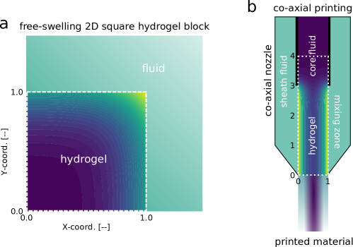
5.1 Benchmark: free-swelling of a 2D square hydrogel block
As a benchmark problem, we consider the transient free-swelling of a gel in a two-dimensional setting as illustrated in Figure 1a. The 2D hydrogel block initially has a square cross-section. The hydrogel block is immersed into a non-reactive solvent with a reference chemical potential . Only a quarter of the whole model is considered because of the symmetry of the block. In terms of mechanical boundary conditions, the bottom and left edges are subject to Dirichlet boundary conditions and , respectively. The top and right edges are considered to be traction-free. In terms of chemical boundary conditions, the bottom and left edges are subject to zero fluid flux. The chemical potential is subjected to a Robin boundary condition as defined in equation (29) on the top and right edges. A similar setup to this example can be found in, e,g., [14], [29], or [12].
The following values are selected as the nominal dimensionless material parameter222Note: The dimensionless material parameters are related to the following physical material parameters through equations (23): [m], [J], [m3], [m2/s], [kPa], and [kPa].: and , and the Robin boundary coefficient is defined as . The chemical potential’s initial condition is , and the domain is considered to be initially stress-free. The material parameters were taken from the experimental work of [12] and represent a gelatin-based hydrogel. The reader is referred to [12] for more details on gel preparation and mechanical characterization.
The domain is discretized into triangular elements with quadratic interpolation for displacement and linear interpolation for the chemical potential to obtain the Taylor-Hood elements as introduced in Section 2. The dimensionless coupled system of equations (33) is solved as a variational monolithic problem using the FEniCS package as a PDE solver.
Following the convergence analysis reported in A, a mesh density of , i.e., triangle elements, is specified to obtain what we denote as the FOM nominal simulation setup. The total dimensionless simulation time is chosen as , and the time interval is discretized into time steps.
5.1.1 Numerical results for the full-order model
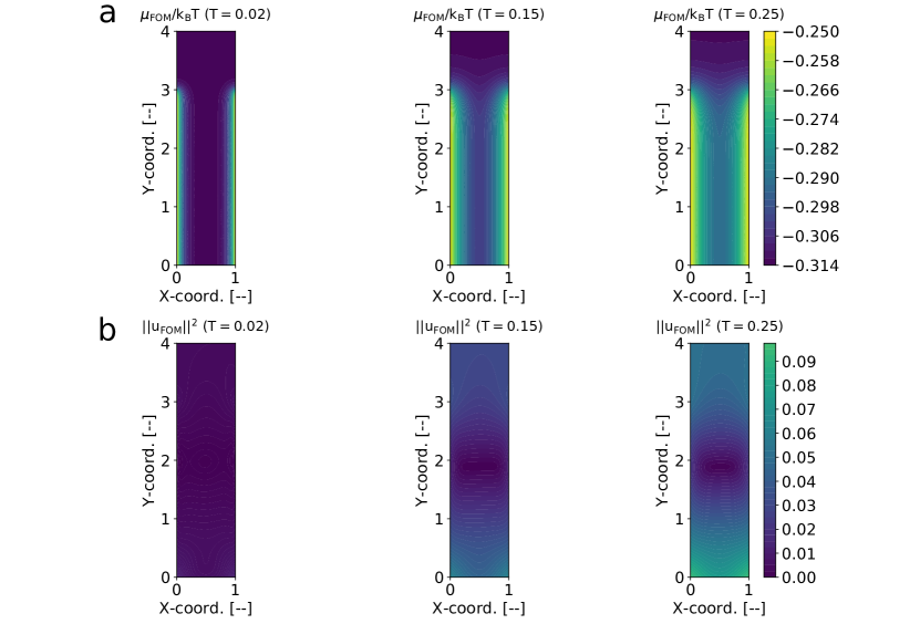
Figures 2 and 3 show the primary variables and postprocessing quantities for the FOM at three different simulation times. Figure 2a displays the evolution of the chemical potential within the 2D hydrogel block. It can be observed that the chemical potential transitions over time from its initial condition to its boundary value. This increase in chemical potential indicates that as the gel absorbs the solvent, its internal fluid concentration rises, driving the absorption process toward equilibrium.
Figure 2b illustrates the evolution of the displacement magnitude. It is evident that displacement increases in tandem with solvent absorption, with the highest displacement occurring in the corner fully exposed to the solvent. The symmetry in the displacement field reflects the isotropic swelling of the gel.
Figure 3 presents strain and normalized stress, computed from equations (2) and (31), respectively. Only and are shown, but due to the symmetry of the displacement field, and exhibit a similar profile and are thus not depicted here. From Figure 3a, we see that is highest on the solvent-exposed side but tends to increase throughout the domain as time progresses. Conversely, as seen in Figure 3b, is zero at the exposed boundary on the right, indicating that the boundary remains traction-free throughout the simulation, while it increases towards the center of the gel block and decreases at the top boundary. The increase in stress towards the center suggests that as the gel absorbs the solvent, it swells, leading to internal stresses due to the material’s expansion, constrained by its own structure. The observed decrease in stress at the top boundary suggests reduced solvent absorption in the direction at this location, consistent with expectations of greater absorption in the direction. This pattern aligns with the directional swelling behavior of the gel, where absorption predominantly occurs in the Y direction at the top boundary.
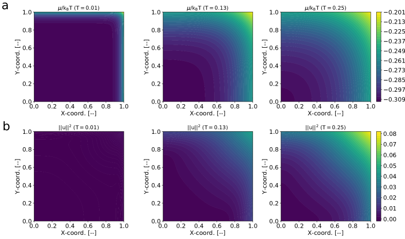
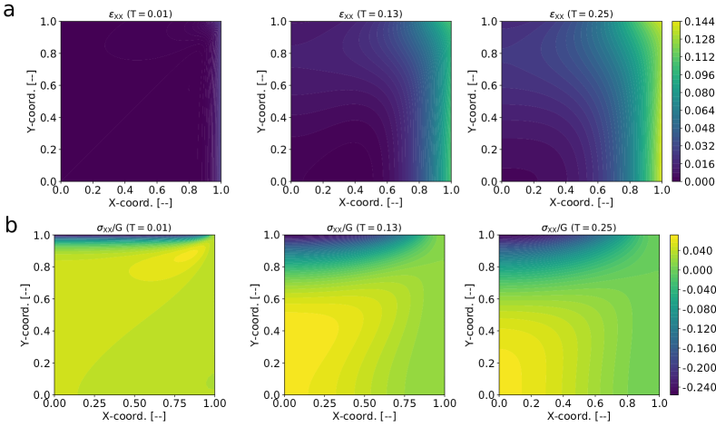
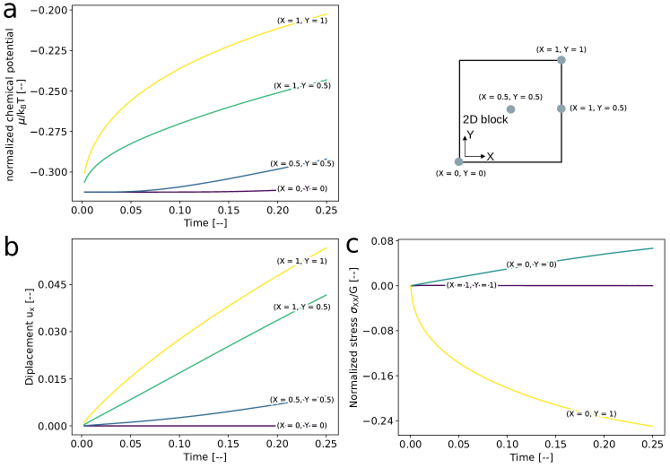
Figure 4 shows the time evolution of normalized chemical potential (Figure 4a), displacement (Figure 4b), and normalized stress (Figure 4c) at different points in the 2D hydrogel block. The figure reveals that the four selected points undergo different diffusion-deformation pathways, highlighting the spatial dependency of the problem. Figure 4 complements observations from Figures 2 and 3. Figure 4c reaffirms that the points on the right side remain traction-free throughout the simulation.
Material parameter variation effect analysis
The linear diffusion-deformation theory adopted in this work defines a hydrogel in terms of two dimensionless parameters as stated in the constitutive equation (31), namely and . Note that [12] also studied this problem and conducted some experimental work to validate their mathematical model. Their findings showed that the material parameters could present a significant source of uncertainty under a similar gel fabrication protocol (the reader is referred to Figures 3 and 5 in [12]).
In order to understand the effect of the material parameters on the simulation outcome, the FOM is repeatedly simulated varying one of the parameters at a time, while keeping the others constant. This allows us to analyze the temporal evolution of the primary variables as well as of the average strain for each of the parameter combinations. The average strain is given by
| (53) |
with the 2D block area and representing the differential area element.
To understand the influence of , we vary it uniformly from 2000 to 6000, while keeping fixed at its nominal value. Conversely, to evaluate the influence of a variation in , we vary uniformly from 1000 to 2000, while keeping fixed at its nominal value. The dimensionless simulation time is increased to to better illustrate the effect of the material parameter variation. Everything else is kept the same as reported above for the nominal FOM simulation.
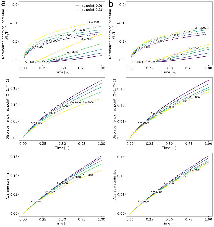
Figure 5 depicts the effect of varying (column a) and (column b) on the temporal evolution of the primary variables, namely, the normalized chemical potential and the displacement in direction. Moreover, the effect on the temporal evolution in the average strain is investigated. The first row in Figure 5 displays the temporal evolution of the normalized chemical potential at the corner that is fully exposed to the solvent () as well as at the symmetry corner (). The second row shows the effect of varying (column a) and (column a) on the displacement in direction at the fully exposed corner (). The third row reports the effect of varying the material parameters over the temporal evolution of the average strain . From Figure 5 can be appreciated that variations in the material parameters can lead to considerable differences in the diffusion-deformation process evolution. The effect of varying becomes more pronounced than that of as time progresses, but neither the effect of nor can be neglected.
5.1.2 Numerical results for the reduced-order model
In this section, we provide numerical experiments to validate and demonstrate the accuracy and computational efficiency of the ROM. All the following computations are conducted in RBniCS.
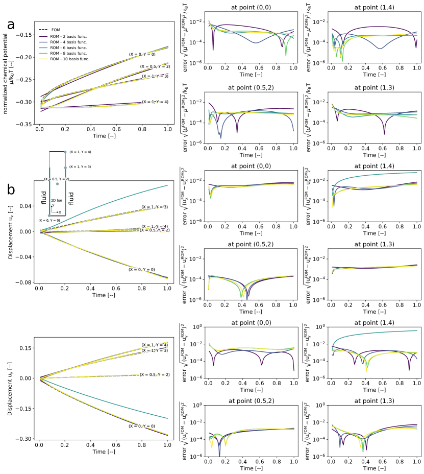
The same mesh density and time steps as for the nominal simulation are taken. Material parameters are varied as reported in Figure 6. samples are taken from the parameter space creating a total snapshots dataset of , i.e., snapshots in total. The ROM is assembled by increasing the number of basis functions. Some locations at the 2D square domain are selected to verify the ROM’s accuracy as indicated in Figure 6. The root mean square error (RMSE) is measured over time at each location.
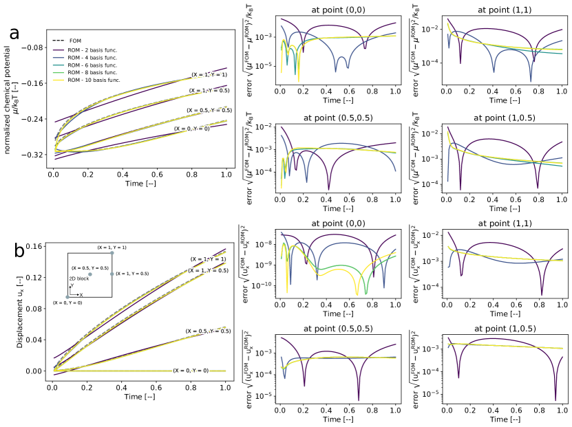
The ROM for the 2D hydrogel block developed using the nested-POD method is compared with the nominal FOM model ( and ) because they were not included in the training dataset. Figure 6 depicts a comparison of the temporal evolution of chemical potential (Figure 6a) and displacement (Figure 6b) at different points inside the 2D hydrogel block for an increasing number of POD basis functions. The figures show that the maximum RMSE between both models remains below in most cases for the chemical potential and displacement. This threshold is only exceeded when only two basis functions are used. Among all the observed points, the error is highest at the beginning of the simulation at the fully exposed corner (), but it alternates as time evolves. In some cases, the error decreases over time for the chemical potential and displacement. In summary, we conclude that using six basis function leads to the best trade-off between the ROM complexity and accuracy for the 2D square block case.
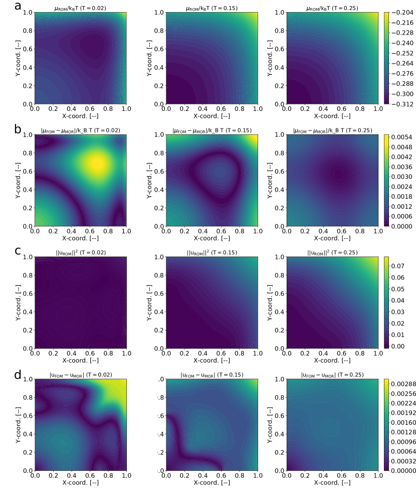
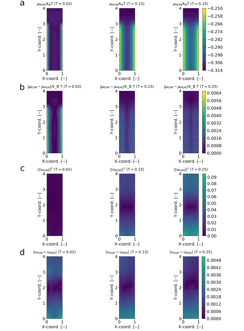
Figure 7 displays the chemical potential (Figure 7a) and displacement (Figure 7c) obtained with the six basis functions at three different time steps, namely, . Errors with respect to the FOM simulation results reported in Figure 2 are displayed for the chemical potential in Figure 7b) and for the displacement in Figure 7d. As seen from Figure 7, the ROM can predict the FOM to a satisfactory extent. From Figures 7b and d it can be observed that the maximum discrepancy between the FOM and ROM is less than 0.55% for the chemical potential and 0.3% for the displacement field, respectively. It is also clear that the maximum discrepancy occurs at the beginning of the simulation but fades as time evolves. This result is expected because, at the beginning of the simulation, the chemical potential field has a very sharp gradient close to the exposed boundaries but it is almost flat towards the center. It is well known that global surrogate models suffer when approximating flat functions.
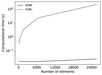
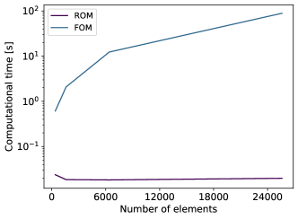
Figure 8 demonstrates the significant computational speed-up achieved with the ROM. For instance, the FOM computation time for is s, but for it is already s. This corresponds to an exponential increase of the computational cost w.r.t the mesh density. In contrast, the ROM computation time for is s, but for it is still only s. That is, the ROM simulation is about factor faster than the FOM simulation for .
5.2 Case study: co-axial hydrogel bioprinting
In this section, we present the implementation of the ROM for a case study closely resembling a bioprinting process. It corresponds to what is known as co-axial hydrogel printing, which involves a dual-nozzle system for the simultaneous extrusion of a hydrogel precursor and a crosslinking agent, enabling immediate gelation and structural integrity. Coaxial printing provides a basic core/sheath printing configuration (see the schematic representation in Figure 1b), which can be adapted to fit the design considerations of the desired 3D structure. Coaxial bioprinting can be used to control concentric multi-material deposition or improve resolution through inline crosslinking. This technique is crucial in tissue engineering for creating complex 3D structures with controlled properties like stiffness and porosity [25]. Adjusting material flow rates and compositions allows for fabricating hydrogels with gradient properties, mimicking natural tissue complexity. Despite its potential, co-axial printing faces challenges like maintaining balanced rheological properties and preventing nozzle clogging, necessitating precise control and optimization in the printing process [25]. These limitations can be tackled by combining process modeling and experiments. Developing a ROM mimicking the co-axial printing process would aid in efficiently optimizing the printing parameters and can be adopted within a digital twin framework to monitor and guide the printing process.
5.2.1 Simulation setup
We consider a vertical hydrogel bar where the height is four times the length as marked by the dashed white box in Figure 1b. We assume that the diffusion time of the fluid into the hydrogel is relatively large compared to the velocity at which the hydrogel is extruded out of the printer’s nozzle. This allows us to neglect the physics of the hydrogel transport through the co-axial nozzle. We study the transient free-swelling of the hydrogel bar in a two-dimensional setting, assuming a homogeneous mix of gel and solvent at the nozzle’s tip. The material parameters are the same as in the benchmark problem mentioned earlier. Therefore, if the characteristic length in the previous example is m, the dimensions of the hydrogel bar are m2 or, equivalently, mm2. This size is representative of a filament being crosslinked in the nozzle of a co-axial 3D bioprinter.
We assume that only of the gel bar is exposed to the solvent on the left and right edges, where a Robin boundary condition imposes the chemical potential as defined in equation (29). The remaining of the left and right edges and the top surface have zero fluid flux for the solvent concentration boundary conditions. In terms of mechanical boundary conditions, all other boundaries are considered to be traction-free.
The domain is discretized into triangular elements with quadratic interpolation for displacement and linear interpolation for the chemical potential, resulting in Taylor-Hood elements as introduced in Section 2. Equation (33) is solved as a variational monolithic problem using the FEniCS package as a PDE solver.
5.2.2 Numerical results for the full-order model
Figure 9 presents the evolution of primary variables in the hydrogel bar at different simulation times. In Figure 2a, the chemical potential is shown. Over time, the chemical potential increases from its initial state to match the boundary value, indicating a rise in internal fluid concentration as the gel absorbs solvent.
Figure 2b depicts the displacement magnitude’s evolution. As solvent absorption progresses, displacement increases, with the highest displacement observed at the bottom of the hydrogel bar. Notice that the displacement field is not symmetric. The asymmetry in the displacement field suggests uneven swelling of the hydrogel bar during the printing process. This is relevant because this uneven swelling could impact the mechanical integrity of the final printed structure, particularly in complex multi-layered scaffold designs, where stability is crucial. This is exactly what makes this case study relevant for the bioprinting community.
5.2.3 Reduced-order model
In this section, we provide numerical experiments to validate and demonstrate the accuracy and computational efficiency of the ROM as we did for the benchmark case.
The same mesh density and time steps as for the nominal simulation are taken. Material parameters are varied within the same range as in the benchmark problem (see Figure 6). samples are taken from the parameter space for each of the 100 time steps, creating a total snapshots dataset of , i.e., snapshots in total. The ROM is assembled by increasing the number of basis functions. Four locations at the 2D square domain are selected to verify the ROM’s accuracy as marked in Figure 10. The root mean square error (RMSE) is measured over time at each location.
The ROM for the hydrogel bar developed using the nested-POD method is compared with the nominal FOM model ( and ). This is possible because these nominal values were not included in the training dataset. Figure 10 depicts a comparison of the temporal evolution between ROM and FOM in terms of chemical potential (Figure 10a), displacement in direction (Figure 10b) and displacement in direction (Figure 6c) at different points of the hydrogel bar for increasing number of basis functions. The figures show that the maximum RMSE between both models remains lower than in most cases for the chemical potential and displacement. This analysis suggests that using eight basis functions leads to the best trade-off between ROM complexity and accuracy. In the previous benchmark, only six basis functions were necessary.
Figure 11 displays the chemical potential (Figure 11a) and displacement (Figure 11c) obtained with eight basis functions at three different time steps, namely, . The corresponding errors with respect to the FOM simulation results from Figure 9 are illustrated for the chemical potential in Figure 11b and for the displacement in Figure 11d), respectively.
As seen from Figure 11, the ROM can predict the FOM to a satisfactory extent. From Figures 11b and d can be observed that the maximum discrepancy between the FOM and ROM is less than 0.64% for the chemical potential and 0.48% for the displacement field, respectively.
Figure 12 displays the computation speed-up achieved with the ROM. A FOM computation with 142 elements (coarser mesh) costs s, but with 37174 elements (finer mesh), it already costs s, which means that the computational cost increases exponentially with the mesh density. In contrast, a ROM computation with 142 elements costs s, but with 37174 elements it only costs s. That is, the ROM simulation is times faster than the FOM simulation with the finer mesh.
5.2.4 Material parameter identification from full-field data
This section shows the potential of using the developed ROM to estimate the model’s material parameters from full-field data. In the lack of experimental data, we take the solution of the nominal FOM () at as synthetic data. It is worth recalling that the ROM did not encounter these values in the training dataset.
The optimization problem (49) to identify the optimal value of the material parameters was implemented in Python and solved using the minimize function from the Scipy library [41]. We selected the L-BFGS-B algorithm, a variant of the Limited Memory Broyden–Fletcher–Goldfarb–Shanno (L-BFGS) algorithm, which belongs to the family of quasi-Newton methods [44]. This algorithm is particularly suited for solving large-scale optimization problems with bound constraints.
The optimization process starts with an initial guess for the material parameters, set to , but we verified that the same result is obtained if different initial conditions are chosen. The bound constraints ensure that the solution remains within the parameter range the ROM was trained for.
The hyperparameters of L-BFGS-B algorithms are the maximum number of function evaluations and iterations (‘maxfun’ and ‘maxiter’), both set to . The function tolerance (‘ftol’) is set to , and the gradient tolerance (‘gtol’) to . The function tolerance dictates the precision of the objective function and the convergence criterion based on the gradient’s magnitude, respectively. The step size for numerical approximation (‘eps’) is , and the maximum number of line search steps (‘maxls’) per iteration is . This setup allowed for efficient parameter space exploration while adhering to the constraints imposed by the problem’s physical context.
Table 1 summarizes the results obtained from the parameter identification with ROM and FOM, as well as the related computational cost. From the results, it is possible to observe the ROM’s effectiveness in performing many-query tasks. The material parameters identified with the ROM have a relative error of and for and , respectively. Considering both the ROM training and the actual parameter identification, only a fifth of the time needed with the FOM was consumed. It is important to remark that the material parameter values identified using the FOM also deviate from the nominal values used to create the synthetic data. This discrepancy is attributed to the low number of snapshots used for the identification problem. That is, only two snapshots, , out of the generated with the solution of FOM. If more snapshots were considered for the identification problem, the error between the identified and correct material parameters is expected to decrease, but especially with the FOM, the computational cost would also increase significantly.
| ROM | FOM | |
| model evaluations ROM only training (computation time) | 0 (0h) | 30 (1h) |
| average model evaluations only identification (computation time) | 150 (5min) | 150 (5h) |
| computation time training + identification | 1h + 5min | n.a. + 5h |
| dimensionless first Lamé constant | 1587 | 1493 |
| absol. error | 29 | 65 |
| relative error [%] | 1.86 | 4.16 |
| dimensionless scaling factor | 3916 | 4041 |
| absol. error | 84 | 41 |
| relative error [%] | 2.10 | 1.04 |
6 Conclusions
In this paper, we demonstrated that nested POD is feasible for developing a ROM of the coupled diffusion-deformation model. The accuracy of the ROM was tested in two different scenarios: i. free-swelling of a 2D gel block, a well-established benchmark in the literature, and ii. a case study closely resembling a bioprinting process using a co-axial bioprinter. In both cases, we highlighted the computational benefits of adopting the ROM, where the computational cost of the ROM online evaluation was only 0.01% of running the full-order model. Specifically, we found that the ROM is times faster than the FOM when using a fine mesh to simulate the transient diffusion-deformation evolution in the co-axial printing application. Finally, we showed the benefits of adopting a ROM in a many-query task, that is, parameters identification from full-field data. We showed that the computational resources spent in the offline phase for training data generation and ROM construction are repaid by a relatively large number of evaluations (150 on average) of the trained model in an online phase, i.e., the parameter identification. The significant simulation speed-up provided by the ROM paves the way for more advanced applications, such as online feedback error compensation during the bioprinting process. This would ensure that the printed products meet design and functional requirements, ultimately aiming to produce consistent, high-quality hydrogel products to advance the reliability of bioprinting technologies.
Supplementary information No supplementary information was produced from this research.
Acknowledgments GA gratefully acknowledges the RBniCS developer, Dr. Francesco Ballarin, for his support in the implementation of algorithms for the reduced order model. TW gratefully acknowledges the Deutsche Forschungsgemeinschaft (DFG) under Germany’s Excellence Strategy within the Cluster of Excellence PhoenixD (EXC 2122, Project ID 390833453).
Declarations
Funding: The authors declare that no funds, grants, or other support were received during the preparation of this manuscript.
Conflict of interest/Competing interests: On behalf of all authors, the corresponding author states that there is no conflict of interest.
Code availability: The code to reproduce the results presented in this manuscript will be published on zenodo.org upon acceptance of this manuscript.
References
- \bibcommenthead
- Anand [2015] Anand L (2015) 2014 Drucker medal paper: A derivation of the theory of linear poroelasticity from chemoelasticity. Journal of Applied Mechanics 82(11):111005
- Anand and Govindjee [2020] Anand L, Govindjee S (2020) Continuum mechanics of solids. Oxford University Press
- Ballarin et al [2015] Ballarin F, Manzoni A, Quarteroni A, et al (2015) Supremizer stabilization of POD–Galerkin approximation of parametrized steady incompressible Navier–Stokes equations. Int J Numer Methods Eng 102(5):1136–1161
- Ballarin et al [2022] Ballarin F, Rozza G, Strazzullo M (2022) Space-time POD-Galerkin approach for parametric flow control. In: Handbook of Numerical Analysis, vol 23. Elsevier, p 307–338
- Benner et al [2015] Benner P, Cohen A, Ohlberger M, et al (2015) Model Reduction and Approximation: Theory and Algorithms. SIAM Philadelphia
- Benner et al [2020] Benner P, Schilders W, Grivet-Talocia S, et al (2020) Model Order Reduction: Volume 2: Snapshot-Based Methods and Algorithms. De Gruyter
- Biot [1941] Biot MA (1941) General theory of three-dimensional consolidation. Journal of applied physics 12(2):155–164
- Bouklas et al [2015] Bouklas N, Landis CM, Huang R (2015) A nonlinear, transient finite element method for coupled solvent diffusion and large deformation of hydrogels. Journal of the Mechanics and Physics of Solids 79:21–43
- Brunton and Noack [2015] Brunton SL, Noack BR (2015) Closed-loop turbulence control: Progress and challenges. Applied Mechanics Reviews 67(5):050801
- Caccavo et al [2018] Caccavo D, Cascone S, Lamberti G, et al (2018) Hydrogels: experimental characterization and mathematical modelling of their mechanical and diffusive behaviour. Chemical Society Reviews 47(7):2357–2373
- Chen et al [2015] Chen P, Quarteroni A, Rozza G (2015) Reduced order methods for uncertainty quantification problems. ETH Zurich, SAM Report 3
- Chen et al [2020] Chen S, Huang R, Ravi-Chandar K (2020) Linear and nonlinear poroelastic analysis of swelling and drying behavior of gelatin-based hydrogels. International Journal of Solids and Structures 195:43–56
- Chester and Anand [2010] Chester SA, Anand L (2010) A coupled theory of fluid permeation and large deformations for elastomeric materials. Journal of the Mechanics and Physics of Solids 58(11):1879–1906
- Chester and Anand [2011] Chester SA, Anand L (2011) A thermo-mechanically coupled theory for fluid permeation in elastomeric materials: application to thermally responsive gels. Journal of the Mechanics and Physics of Solids 59(10):1978–2006
- Chester et al [2015] Chester SA, Di Leo CV, Anand L (2015) A finite element implementation of a coupled diffusion-deformation theory for elastomeric gels. International Journal of Solids and Structures 52:1–18
- Eckart and Young [1936] Eckart C, Young G (1936) The approximation of one matrix by another of lower rank. Psychometrika 1(3):211–218
- Eftekhar Azam et al [2017] Eftekhar Azam S, Mariani S, Attari N (2017) Online damage detection via a synergy of proper orthogonal decomposition and recursive bayesian filters. Nonlinear Dynamics 89:1489–1511
- Fareed et al [2018] Fareed H, Singler JR, Zhang Y, et al (2018) Incremental proper orthogonal decomposition for PDE simulation data. Computers & Mathematics with Applications 75(6):1942–1960
- Fischer et al [2024] Fischer H, Roth J, Wick T, et al (2024) MORe DWR: space-time goal-oriented error control for incremental POD-based ROM for time-averaged goal functionals. Journal of Computational Physics p 112863
- Girfoglio et al [2022] Girfoglio M, Quaini A, Rozza G (2022) A POD-Galerkin reduced order model for the Navier–Stokes equations in stream function-vorticity formulation. Comp Fluids 244:105536
- Gräßle and Hinze [2018] Gräßle C, Hinze M (2018) POD reduced-order modeling for evolution equations utilizing arbitrary finite element discretizations. Adv Comput Math 44(6):1941–1978
- Kadeethum et al [2021] Kadeethum T, Ballarin F, Bouklas N (2021) Data-driven reduced order modeling of poroelasticity of heterogeneous media based on a discontinuous Galerkin approximation. GEM-International Journal on Geomathematics 12(1):12
- Kadeethum et al [2022] Kadeethum T, Ballarin F, Choi Y, et al (2022) Non-intrusive reduced order modeling of natural convection in porous media using convolutional autoencoders: Comparison with linear subspace techniques. Advances in Water Resources 160:104098
- Kerschen et al [2005] Kerschen G, Golinval JC, Vakakis AF, et al (2005) The method of proper orthogonal decomposition for dynamical characterization and order reduction of mechanical systems: An overview. Nonlinear Dyn 41(1):147–169
- Kjar et al [2021] Kjar A, McFarland B, Mecham K, et al (2021) Engineering of tissue constructs using coaxial bioprinting. Bioactive materials 6(2):460–471
- Lass and Volkwein [2014] Lass O, Volkwein S (2014) Adaptive POD basis computation for parametrized nonlinear systems using optimal snapshot location. Computational Optimization and Applications 58:645–677
- Lassila et al [2014a] Lassila T, Manzoni A, Quarteroni A, et al (2014a) Model order reduction in fluid dynamics: challenges and perspectives. Reduced Order Methods for modeling and computational reduction pp 235–273
- Lassila et al [2014b] Lassila T, Manzoni A, Quarteroni A, et al (2014b) Model order reduction in fluid dynamics: challenges and perspectives. Reduced Order Methods for modeling and computational reduction pp 235–273
- Liu et al [2016] Liu Y, Zhang H, Zhang J, et al (2016) Transient swelling of polymeric hydrogels: A new finite element solution framework. International Journal of Solids and Structures 80:246–260
- Lu et al [2015a] Lu K, Yu H, Chen Y, et al (2015a) A modified nonlinear POD method for order reduction based on transient time series. Nonlinear Dynamics 79:1195–1206
- Lu et al [2015b] Lu K, Yu H, Chen Y, et al (2015b) A modified nonlinear POD method for order reduction based on transient time series. Nonlinear Dynamics 79:1195–1206
- Lu et al [2016] Lu K, Chen Y, Jin Y, et al (2016) Application of the transient proper orthogonal decomposition method for order reduction of rotor systems with faults. Nonlinear Dynamics 86:1913–1926
- Lu et al [2019] Lu K, Jin Y, Chen Y, et al (2019) Review for order reduction based on proper orthogonal decomposition and outlooks of applications in mechanical systems. Mechanical Systems and Signal Processing 123:264–297
- Negri et al [2013] Negri F, Rozza G, Manzoni A, et al (2013) Reduced basis method for parametrized elliptic optimal control problems. SIAM Journal on Scientific Computing 35(5):A2316–A2340
- Nonino et al [2021] Nonino M, Ballarin F, Rozza G (2021) A monolithic and a partitioned, reduced basis method for fluid-structure interaction problems. Fluids 6(6):229
- Pagani and Manzoni [2021] Pagani S, Manzoni A (2021) Enabling forward uncertainty quantification and sensitivity analysis in cardiac electrophysiology by reduced order modeling and machine learning. International Journal for Numerical Methods in Biomedical Engineering 37(6):e3450
- Sahyoun and Djouadi [2013] Sahyoun S, Djouadi S (2013) Local proper orthogonal decomposition based on space vectors clustering. In: 3rd International Conference on Systems and Control, IEEE, pp 665–670
- Strazzullo et al [2020] Strazzullo M, Zainib Z, Ballarin F, et al (2020) Reduced order methods for parametrized non-linear and time-dependent optimal flow control problems, towards applications in biomedical and environmental sciences. In: Numerical Mathematics and Advanced Applications ENUMATH 2019: European Conference, Egmond aan Zee, The Netherlands, September 30-October 4, Springer, pp 841–850
- Urrea-Quintero et al [2024] Urrea-Quintero JH, Marino M, Wick T, et al (2024) A comparative analysis of transient finite-strain coupled diffusion-deformation theories for hydrogels. Archives of Computational Methods in Engineering –:50. Accepted for publication.
- Vaccaro [1991] Vaccaro RJ (1991) SVD and signal processing, ii. algorithms, analysis and applications. Amsterdam: Elsevier
- Virtanen et al [2020] Virtanen P, Gommers R, Oliphant TE, et al (2020) SciPy 1.0: fundamental algorithms for scientific computing in python. Nature methods 17(3):261–272
- Wloka [1987] Wloka J (1987) Partial differential equations. Cambridge University Press
- Zhang and Khademhosseini [2017] Zhang YS, Khademhosseini A (2017) Advances in engineering hydrogels. Science 356(6337):eaaf3627
- Zhu et al [1997] Zhu C, Byrd RH, Lu P, et al (1997) Algorithm 778: L-BFGS-B: Fortran subroutines for large-scale bound-constrained optimization. ACM Transactions on mathematical software (TOMS) 23(4):550–560
- Zou et al [2018] Zou X, Conti M, Díez P, et al (2018) A nonintrusive proper generalized decomposition scheme with application in biomechanics. International Journal for Numerical Methods in Engineering 113(2):230–251
Appendix A 2D square block - Full-order model convergence analysis
A computational convergence analysis is performed to investigate the robustness and computational cost of the monolithic approach. We focus on investigating the effect of mesh density and the time step size on the behavior of the implemented numerical algorithm. We aim to understand how these parameters influence the performance of the algorithm in solving the linear system of equations associated with the FEM discretization.
We test whether using Taylor-Hood elements and the first-order implicit Euler method leads to the expected convergence in space and time. Specifically, we measure the and errors in space for various mesh densities and time step sizes with respect to the highest fidelity solution. That is,
| (54) |
for the displacement, with being a reference solution obtained using a very fine mesh and the obtained displacement obtained for either different mesh or time step sizes.
Figure 13 shows the and error norms, evaluated as both mesh size (Figure 13a) and time steps (Figure 13b) are refined. The errors are calculated against a benchmark of a fine mesh and small time steps. For the spatial dimension, the error analysis involves refining from a coarser mesh to a finer mesh. For the temporal dimension, the refinement process starts with time steps and increases to , discretizing the dimensionless time interval more finely. From Figure 13, it is observed that in both cases the error keeps decreasing as mesh size and time steps refine.
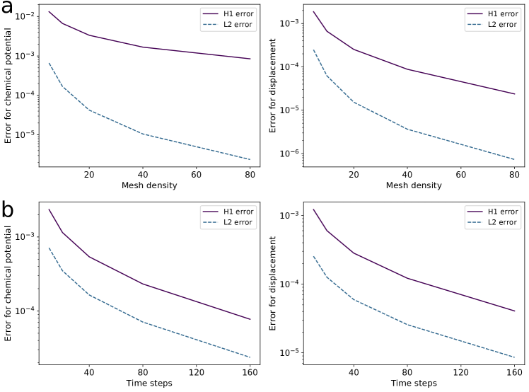
We estimate the convergence order of the numerical method implemented with a well-known heuristic formula. Let us denote the errors by , , and , where is the mesh size parameter as before. Under the assumption that our discretized problem has a convergence order of , then each error should be roughly times the previous error. Therefore, we can estimate by taking the logarithm base of the error ratios as:
| (55) |
The computational convergence analysis is detailed in Table 2. From finite element interpolation estimates for non-coupled problems and with optimal regularity of coefficients, we expect for polynomial shape functions of degree in the norm the order and in the norm . In the temporal direction, the first order implicit Euler scheme has the order , irrespectively of the spatial evaluation means. Thus, the temporal convergence analysis results are nearly optimal, as observed in Table 2. For the spatial analysis, for the non-coupled case with optimal regularity assumptions, we would expect for the order in the norm and order in the norm. Furthermore, we would expect for the order in the norm and order in the norm, and, finally, we would expect for the order in the norm and order in the norm. Specifically, we come close to these orders for the chemical potentials. For the displacements, we have slightly less optimal orders. However, our main assumption in these theoretical expectations was non-coupled partial differential equations with optimal regularity assumptions in the coefficients, the domain, the boundary, and the given problem data. Due to the nonlinear coupling, it is likely that the optimal orders are not achieved. Nonetheless, our findings certainly point in the right direction and clearly serve the purpose of the robust finite element verification of the full-order model.
| Convergence order | (degree=2) | (degree=3) | (degree=1) | (degree=2) | |
| Space | norm | 2.3222 | 3.4899 | 1.9623 | 2.9713 |
| norm | 1.6617 | 2.5822 | 0.9646 | 1.9801 | |
| Time | norm | 0.9462 | – | 0.9631 | – |
| norm | 0.9610 | – | 0.9735 | – |