Deep Learning Based Dynamics Identification and Linearization of Orbital Problems using Koopman Theory

Abstract

The study of the Two-Body and Circular Restricted Three-Body Problems in the field of aerospace engineering and sciences is deeply important because they help describe the motion of both celestial and artificial satellites. With the growing demand for satellites and satellite formation flying, fast and efficient control of these systems is becoming ever more important. Global linearization of these systems allows engineers to employ methods of control in order to achieve these desired results. We propose a data-driven framework for simultaneous system identification and global linearization of both the Two-Body Problem and Circular Restricted Three-Body Problem via deep learning-based Koopman Theory, i.e., a framework that can identify the underlying dynamics and globally linearize it into a linear time-invariant (LTI) system. The linear Koopman operator is discovered through purely data-driven training of a Deep Neural Network with a custom architecture. This paper displays the ability of the Koopman operator to generalize to various other Two-Body systems without the need for retraining. We also demonstrate the capability of the same architecture to be utilized to accurately learn a Koopman operator that approximates the Circular Restricted Three-Body Problem.

Two-Body, Circular Restricted Three-Body, Koopman Theory, Neural Network, Linearization

1 INTRODUCTION

The rapid growth in motivation to explore space in the last fifteen years has sparked a number of significant missions to planets such as Mars and Venus, moons such as Enceladus and Titan, as well as our own Moon. From interplanetary missions to the placement of satellites within our own planet’s orbit, we would not be able to achieve the goals of these endeavors without understanding and exploiting the natural dynamics of these systems. Much effort has been spent in determining how exactly the dynamics of bodies, either natural or man-made, are influenced, and how engineers can develop guidance, navigation, and control systems to complete these extraordinary tasks. Today, thousands of satellites orbit around our Earth in a variety of different orbits, and the governing equations of motion for all of these satellites are the equations originating from the N-Body Problem. In the N-Body equations of motion, the only force that imparts energy onto the bodies is gravity [1], and dependent on the complexity of the solution required and the nature of the system in question, the number of bodies varies. Most often in celestial dynamics, the Two-Body Problem (2BP) and Circular Restricted Three-Body Problem (CR3BP) are analysed and used [2, 3, 4, 5, 6, 7, 8, 9, 10, 11]. As we endeavour to reach the Moon again, and move forth to Mars, the analysis and use of the CR3BP will become even more prevalent [7, 10, 11].

In the case of artificial satellites orbiting Earth, they are all governed by the 2BP with perturbations [12, 13]. With the growing number of these satellites being put into orbit, as seen with the explosion of SpaceX Starlink satellites, the need for a fast, efficient and guaranteed method for propagating and controlling the complex dynamics of these bodies is becoming more evident. The linearization of the 2BP has been achieved through the Clohessy-Wiltshire relative motion equations [14], under extensive assumptions, but the discovery of a globally linear representation of this problem has yet to be uncovered.

The case of the CR3BP is a well-known and studied reduction of the Three-Body problem, to which no global analytical solutions exist [7, 10, 11]. Instead, quasi-periodic, periodic and hyperbolic invariant manifolds present themselves as special solutions, which can inform us on the dynamics of the CR3BP [5, 15, 7, 10, 11]. This system is of importance because the Earth-Moon system can be treated as such [8], with the orbit of the Moon around the Earth having an eccentricity of 0.0549 [16]. The Earth-Moon system has five equilibrium points, the so-called Lagrange points [9], around which it is possible to generate periodic orbits that are intergrable. Much like the 2BP, efficient, accurate linear representation of the CR3BP would further advance the exploration of space, by reducing the complexity of creating control systems capable of being used in these systems.

The control of nonlinear systems has long been a challenge for engineers. Linear control systems often have straightforward and useful methods in order to achieve theoretical guarantees in the controllability, observability, and stability of the system. Current techniques provide some relief to this problem, however the horizon upto which these techniques can be relied on is measurably short. This leads to frequent linearization calculations around specific operating points, increasing computational cost and time when performing control maneuvers and state estimation. A globally linear representation of the dynamics of the system would be an ideal solution, eliminating the drawbacks of traditional linearization techniques. Unfortunately, finding such global linearizations is still a prominent issue, but with the recent advancements in Koopman theory, the prowess of machine learning and advancements in computational power, this ideal solution may not be as unattainable as once thought.

Koopman theory, first proposed in 1931 [17], has gained traction over the last few years as a solution for finding global linearization of nonlinear systems. In a nutshell, the theory states that the dynamics of a nonlinear system can be described linearly by an infinite-dimensional Koopman operator. Due to its infinite dimension, for practical use, it is typically approximated using data-driven methods such as Extended Dynamic Mode Decomposition (EDMD) [18]. The process of implementing EDMD on the nonlinear system to find an accurate approximation is not only highly involved, but requires an innate understanding of the method in order to select the basis functions. These basis functions are the building blocks from which functions known as observable functions are constructed. These observable functions are then what is applied to the data in order to lift dynamics to the appropriate dimension. However, constructing a feed-forward neural network (NN) that implements EDMD makes it possible to find an approximate general Koopman operator linearization applicable to a region of state space, that is time invariant and constant. Another advantage of using a data-driven method is that it does not require system knowledge, and the nonlinear system can be completely unknown [19, 20].

Neural Networks, although having a history that spans almost 40 years, have found a resurgence in the last 10-15 years, propelled by the work of LeCun et al. [21], who were able to analyse the ImageNet dataset and accurately categorize image classes within the dataset. Since then, the advancements of big data coupled with computational power has allowed Deep Neural Networks (DNNs) to grow rapidly, and be integrated into many fields of research and development. The power of DNN’s lies in their ability to represent any arbitrary function, including the Koopman observable functions required to linearize the nonlinear dynamics [22]. This is possible through a DNN with an adequate number of hidden neurons and a linear output layer, satisfying the universal approximation theorem [23, 24, 25]. The use of a DNN in the approximation of the Koopman operator relieves us from the need to determine a satisfactory set of basis functions to which the Koopman eigenfucntions are mapped from, which is often difficult and can lead to poor approximations if not chosen correctly.

The linearization of orbital (two and three-body) dynamics is an application where this global linearization can be highly beneficial for mission engineering. By reducing the computational cost, already limited CPU power can be diverted to more demanding tasks. In particular, a Koopman framework could be used in order to perform the state estimation tasks required for close-proximity maneuvers such as cluster formation, orbital changes, station keeping and rendezvous. In recent years, the rising abundance of satellite clusters associated with projects such as SpaceX’s Starlink network and LISA (Laser Interferometer Space Antenna) [26, 27] have revived the need for a fast, efficient and guaranteed control of satellites relative to one another.

Numerous advancements in the framework are similar to the one presented in this paper. Not only does the model generate a globally linear, time-invariant representation of the nonlinear dynamics, removing the need for applications of system identification, but we can also use this model’s prediction capability to work as a state estimator, eliminating the need for a Kalman Filter or its variants. The now globally linear system also no longer requires the burden of frequent linearizations such as Taylor Series expansions. In the case of the 2BP, assumption-heavy and limiting equations such as the Clohessy-Wiltshire equations may now be discarded in favor of this linear system.

This work extends the framework developed in Tiwari et al. [28]. The framework of the DNN developed by Tiwari et al. is kept the same, with improvements added for this application. Although the application included control, it is not incorporated for the purposes of this paper when the methodology is applied to both the 2BP and CR3BP. To the best of our knowledge, this is the first time that both the 2BP and the CR3BP have been globally linearized with reasonable precision.

The contributions of this paper are twofold:

• First we demonstrate the ability of the learned Koopman operator to globally linearize a Circular Two-Body problem centered around the Earth for orbits with an apogee altitude ranging between 200-30000km. We also demonstrate the ability of the same network, without additional training, to generalize to other two body systems, specifically around the Moon and Jupiter. We demonstrate that the approximation is accurate and that various invariant properties of the circular orbit are conserved.

• Second, we demonstrate the applicability of the Koopman operator to the more complicated Circular-Restricted Three-Body Problem (CR3BP). We globally linearise the periodic orbit of a satellite that orbits the Earth, including the influence of the Moon, with the initial position of the satellite being close to the L1 Lagrange point. We also analyze the accuracy of the approximation by studying the conservation of the Jacobi constant in the CR3BP, showing that our model can adequately capture the value of this constant throughout the evolution of the dynamics.

2 NONLINEAR DYNAMICS AND THE KOOPMAN OPERATOR

2.1 Koopman Operator Theory

2.1.1 Koopman Operator

The Koopman operator theory states that a nonlinear dynamical system can be transformed into an infinite-dimensional linear system [17]. Consider a dynamical system; the nonlinear, continuous dynamics are propagated by the following mathematical expression:

$$\frac{d}{dt}\boldsymbol{x}(t)=\boldsymbol{F}(\boldsymbol{x}(t))$$ (1)

where, $\boldsymbol{x}(t)\in\mathbb{R}^{n}$ is the system state at time $t$ and $\boldsymbol{F}$ is the function that describes the evolution of the state in the continuous sense. This continuous system can also be modelled in a discrete-time representation by evaluating the solution to the system at finite, discrete time intervals $\Delta t$, such that $\boldsymbol{x}_{k}=x(k\Delta t).$ Hence, the discrete-time dynamics are represented as:

$$\boldsymbol{x}_{k+1}=\boldsymbol{f}(\boldsymbol{x}_{k})$$ (2)

where $\boldsymbol{x}_{k}\in\mathbb{R}^{n}$ is the system state, $k$ is the current time step, and $\boldsymbol{f}$ is the function that evolves the system states through state space. We can then define observables, which are real-valued functions of the system state: $g:\mathbb{R}^{n}\rightarrow\mathbb{R}$ such as: $[x^{2},x^{3},sin(x),cos(x)]$ for instance. The continuous time Koopman operator, $\mathcal{K}$ and discrete time operator $\mathcal{K}_{\Delta t}$, is therefore defined such that, for any observable function $g$,

$$\mathcal{K}g=g\circ\boldsymbol{F},$$ (3)

$$\mathcal{K}_{\Delta t}g(\boldsymbol{x}_{k})=g(\boldsymbol{f}(\boldsymbol{x}_{k}(t)))$$ (4)

where $\circ$ is the composition operator (explicitly defined in 6). We can now apply this operator to the continuous and discrete-time system defined previously to arrive at:

$$\mathcal{K}g=g\circ\boldsymbol{F}(\boldsymbol{x}(t))=\frac{d}{dt}g$$ (5)

$$\mathcal{K}_{\Delta t}g(\boldsymbol{x}_{k})=g(\boldsymbol{f}(\boldsymbol{x}_{k}))=g(\boldsymbol{x}_{k+1}).$$ (6)

It is evident in Equation 6, that the Koopman operator $\mathcal{K}_{\Delta t}$, propagates the observable function of a state $g(\boldsymbol{x}_{k})$ through time to the next time step. An important note is that for this work, we only require use of the discrete-time dynamics, and all further reference to $\mathcal{K}$ is in the discrete-time sense [29]. However, an impractical limitation of this operator is that it is formed in an infinite-dimensional space, therefore, numerical methods are required in order to approximate the operator in a finite dimensional space so that we may be able to access its utility in the control and evolution of dynamic systems.

2.1.2 Dynamic Mode Decomposition and its Extensions

Determining the set of observable functions that span a Koopman invariant subspace, required to lift the states, is not a trivial task. Hence, a number of methods have been derived such as Dynamic Mode Decomposition (DMD), which aims to extract the dynamic modes of a given set of data. These modes can be interpreted as the generalization of the global stability modes and therefore project the underlying physcial mechanisms of the system [30].

DMD has also been extended into Extended Dynamic Mode Decomposition (EDMD), allowing better approximations of the Koopman eigenvalues and eigenfunctions of the system, hence a closer representation of the nonlinear system [18, 31]. Essentially DMD is an approximation using monomial basis functions, analogous to a first-order Taylor expansion, whilst EDMD retains a higher number of terms in the expansion, thus allowing for a better approximation of a wide array of problems.

In all applications of DMD, it is worth noting that the observable functions are built from a set of basis functions. These basis functions which can be any set of functions, such as monomials, radial basis functions (RBF’s) or any other combination, are often chosen by the user. There is a strong connection between the basis functions and DMD’s ability to learn the eigenfunctions and eigenvalues needed to create a more accurate representation of the Koopman operator [20]. Hence, it is largely critical that the determination of the basis functions be made correctly.

2.1.3 Koopman Approximation Algorithm

In this work, the finite dimension Koopman operator is approximated using the combination of EDMD with deep neural networks (DNNs). The procedure in which this is achieved is based off of our method in our previous work, [28], with the work presented herein being an extension of the architecture and structure presented previously. The DNN is used in order to learn and define the set of observables that are used to lift the states, contrary to other methods in which these observable functions are selected manually as a dictionary [32, 33, 34]. Subsequently, the finite-dimensional approximation to the Koopman operator is calculated by utilizing least-squares regression (see Algorithm 1) [28].

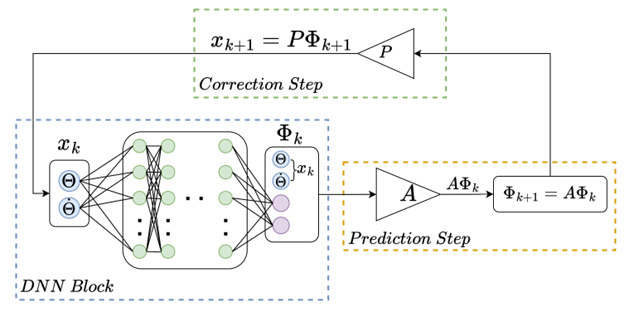
Figure 1: Deep learning framework including the prediction and correction steps. [28]

Algorithm 1 Learning Koopman and Input Matrix

1:Input: X,Y training data, batch size $b_{s},$ Epoch_max

2:Method

3:for epoch in range(Epoch_max) do

4:     for batch in range(number of batches) do

5:         Sample $b_{s}$ from training, control and label

6:            data.

7:            $X=\{X^{i}_{0:k-1}\}^{b_{s}}_{i=1},Y=\{Y^{i}_{1:k}\}^{b_{s}}_{i=1}$

8:         Encode the training and label data and stack

9:            the original states onto the encoded states.

10:            $\Phi_{x}=[X;\Phi(X)]^{T},\Phi_{y}=[Y;\Phi(Y)]^{T}$

11:         Compute the K matrix using EDMD.

12:            $K=\Phi_{y}\cdot(\Phi_{x})^{\dagger}$

13:         Compute the next state with the linear

14:            equation.

15:            $\hat{\Phi}_{x+1}=K\Phi_{x}$

16:         Apply the loss function $\mathcal{L}$ using MSE

17:         Update the model weights and parameters

18:            with the Adam optimizer.

19:     end for

20:end for

21:Output: K matrix, trained DNN

For any non-control affine system, the nonlinear dynamics are propagated by Equation 2. After lifting the states to higher dimension with the observable function, $\boldsymbol{\Phi}$, we desire to find a linear system representation:

$$\mathbf{\Phi}(\boldsymbol{x}_{k+1})\approx\mathbf{K}\boldsymbol{\Phi}(\boldsymbol{x}_{k}),$$ (7)

where the matrix $\mathbf{K}$ approximates the Koopman operator. This matrix is analogous to $\mathbf{A}$, the linear state transition matrix. The goal of the deep learning framework (Fig. 1) is to learn $N$ observables and calculate the $\mathbf{K}$ matrix through the appropriate construction of the loss functions. Because we need to approximate an infinite dimensional operator, we choose $N$ such that $N>>n$ is satisfied, and define

$$\mathbf{\Phi}(\boldsymbol{x}_{k}):=\begin{bmatrix}\boldsymbol{x}_{k}\\ \phi_{1}(\boldsymbol{x}_{k})\\ \phi_{2}(\boldsymbol{x}_{k})\\ \vdots\\ \phi_{N}(\boldsymbol{x}_{k})\end{bmatrix},$$ (8)

where $\phi_{i}:\mathbb{R}^{n}\rightarrow\mathbb{R},i=1,...,N$ are the observable functions, learned by the DNN. An important observation is that we take the observables from the DNN and concatenate the original states $\mathbf{x}_{k}$ on top, helping in two ways: (1) the original states can be easily extracted from the new set of observables (see below), and (2) valuable computational resources can be saved since there is no need for a decoder to recover the original states.

Currently, there is no generalized method to govern the size of $N$ that would guarantee the optimal balance between simplicity and accuracy in the approximation of the Koopman operator; therefore, most often, $N$ is chosen empirically through trial and error. There has been an increase in research that investigates ways to determine the size of $N$ in both controllable and uncontrollable systems [35, 22]. In this work, DNNs are applied with EDMD to approximate the Koopman operator.

To calculate the approximate Koopman operator $\mathbf{K}$, the time history of measurement data for $M$ steps is arranged into snapshot matrices. The first snapshot matrix, $X$, is the state history from time $k=1$ to $k=M-1$, whilst the second snapshot, $X^{\prime}$ is exactly the same as $X$ but shifted forward one time-step:

$$X=\begin{bmatrix}\boldsymbol{x}_{1},\boldsymbol{x}_{2},\boldsymbol{x}_{3},\dots,\boldsymbol{x}_{M-1}\end{bmatrix}$$ (9)

$$X^{\prime}=\begin{bmatrix}\boldsymbol{x}_{2},\boldsymbol{x}_{3},\boldsymbol{x}_{4},\dots,\boldsymbol{x}_{M}\end{bmatrix}$$ (10)

Mapping the measured states, $X,X^{\prime}$ with observable functions leads to

$$\boldsymbol{\Phi}(X)=\begin{bmatrix}\boldsymbol{\Phi}(\boldsymbol{x}_{1}),\boldsymbol{\Phi}(\boldsymbol{x}_{2}),\dots,\boldsymbol{\Phi}(\boldsymbol{x}_{M-1})\end{bmatrix}$$ (11)

$$\boldsymbol{\Phi}(X^{\prime})=\begin{bmatrix}\boldsymbol{\Phi}(\boldsymbol{x}_{2}),\boldsymbol{\Phi}(\boldsymbol{x}_{3}),\dots,\boldsymbol{\Phi}(\boldsymbol{x}_{M})\end{bmatrix}$$ (12)

Given the dataset, the matrix $\mathbf{K}$ can be found by using the least-squares method to minimize the following:

$$\min\sum\left\|\boldsymbol{\Phi}(\boldsymbol{x}_{k+1})-\mathbf{K}\boldsymbol{\Phi}\left(\boldsymbol{x}_{k}\right)\right\|^{2}$$ (13)

Applying the snapshot matrices of real data yields

$$\boldsymbol{\Phi}(X^{\prime})\approx\mathbf{K}\boldsymbol{\Phi}(X)$$ (14)

therefore, on inversion, we end up with

$$\mathbf{K}=\boldsymbol{\Phi}(X^{\prime})\boldsymbol{\Phi}(X)^{\dagger}$$ (15)

where the symbol $\dagger$ denotes the Moore-Penrose inverse of the matrix [36].

Because the Koopman operator calculated in this approach represents an approximation to the real, infinite dimensional operator, and as the observable functions do not span a Koopman invariant subspace, the predicted state is denoted with a circumflex (hat) symbol to emphasise that it is an approximation:

$$\hat{\mathbf{\Phi}}(\boldsymbol{x}_{k+1})=\mathbf{K}\hat{\mathbf{\Phi}}(\boldsymbol{x}_{k})$$ (16)

Now, we can extract the original states from the observables using a projection matrix $\mathbf{P}$ [37], yielding

$$\boldsymbol{x}_{k+1}=\mathbf{P}\hat{\mathbf{\Phi}}(\boldsymbol{x}_{k+1})\;\text{with}\;\mathbf{P}=\begin{bmatrix}\mathbf{I}_{n},\mathbf{0}_{n\text{x}N}\end{bmatrix},$$ (17)

where $\mathbf{I}_{n}$ is the $n\times n$ identity matrix and $\mathbf{0}_{n\times N}$ is the $n\times N$ zero matrix. As shown in [37] and [38], the observable functions not spanning a Koopman invariant subspace accumulate error over time, which leads to predictions with high inaccuracy. However, this error can be mitigated if the prediction is corrected at each time step. This correction is applied by extracting the estimated state variable $\hat{x}_{k+1}$ at each time step with Equation 17, and then reapplying the observable lifting functions to the extracted state variable with Equation 8.

2.2 Circular Orbital Dynamics

One of the two main applications of the proposed model in this work is to linearize a circular 2BP orbit. Orbiting satellites in Low Earth Orbit (LEO) range in altitude from 200-300km to around 2000km [39], and have an eccentricity of less than 0.25, whilst Geostationary orbiting satellites have an ideal eccentricity of 0 [40]. With many of the operational satellites having an eccentricity so close to zero, this aspect motivates us to investigate the linearization of those orbits that are circular, i.e., with zero eccentricity. The equations of motion for a satellite in any orbit is a second-order differential equation that relates the movement of the satellite to the accelerations that perturb the orbit. These accelerations can depend on a number of parameters such as time $t$, position $\vec{\mathbf{r}}$, velocity $\vec{\mathbf{v}}$ or physical forces $\vec{\mathbf{f}}$.

The equation of motion for a two-body orbit is given as follows:

$$\vec{\ddot{\mathbf{R}}}_{2}-\vec{\ddot{\mathbf{R}}}_{1}=-G(M+m)\frac{\vec{\mathbf{R}}_{2}-\vec{\mathbf{R}}_{1}}{\left\|\vec{\mathbf{R}}_{2}-\vec{\mathbf{R}}_{1}\right\|^{3}}+\vec{\mathbf{a}}$$ (18)

Where, $G$ is the Gravitational Constant, $M$ is the mass of the central body, $m$ is the mass of the orbiting body (satellite), $\vec{\mathbf{R}}_{2}-\vec{\mathbf{R}}_{1}$ is the distance from center of the satellite to the central body and $\mathbf{a}$ is the additional perturbing acceleration. In our work, we set $\mathbf{a}=\vec{\mathbf{0}}$ to preserve the circularity of the orbit, which should improve the DNN’s ability to learn the observables, consequently leading to a more accurate representation of the Koopman operator. To prove the ability of the model, we simplify the nonlinear dynamics by choosing not to include orbital perturbations such as drag, solar radiation pressure, or a complex gravity model such as the J2 perturbation model, but they can be included in the nonlinear dynamics, at the expense of a potentially larger K matrix. We also set the position of the central body, $\vec{\mathbf{R}}_{1}$, to be at the origin, hence simplifying 18 to:

$$\vec{\ddot{\mathbf{r}}}=\mu\frac{\vec{\mathbf{r}}}{\left|\vec{\mathbf{r}}\right|^{3}}$$ (19)

where $\mu=-G(M+m)$ is defined as Earth’s gravitational parameter. Note that because $M>>m$, the mass of the satellite is often ignored in the calculation of $\mu$; however, in our work, it is still taken into account and the abbreviation is held as such.

We choose to represent the orbits as in-plane, thus in two dimensions [9, 41], resulting in $z=0$ for all time. This results in four states being required to represent the nonlinear system in state space:

$$\mathbf{x}=\begin{bmatrix}x_{1}\\ x_{2}\\ x_{3}\\ x_{4}\end{bmatrix}=\begin{bmatrix}x\\ y\\ \dot{x}\\ \dot{y}\end{bmatrix}$$ (20)

And the state space representation of the nonlinear model would correspond to:

$$\dot{\mathbf{x}} =\begin{bmatrix}\dot{x_{1}}\\ \dot{x_{2}}\\ \dot{x_{3}}\\ \dot{x_{4}}\end{bmatrix}=\begin{bmatrix}\dot{x}\\ \dot{y}\\ \ddot{x}\\ \ddot{y}\end{bmatrix}$$ (21)

$$=\begin{bmatrix}0&0&1&0\\ 0&0&0&1\\ \frac{\mu}{\left|\vec{\mathbf{r}}\right|^{3}}&0&0&0\\ 0&\frac{\mu}{\left|\vec{\mathbf{r}}\right|^{3}}&0&0\end{bmatrix}\begin{bmatrix}x_{1}\\ x_{2}\\ x_{3}\\ x_{4}\end{bmatrix}$$

To ease the generation of data for this system, each orbit obtains the same initial pose, being,  $x=r,y=0$. Hence, the initial velocity is purely tangential, resulting in the initial velocities being:

$$\dot{x}=0$$ (22)

$$\dot{y}=\sqrt{\frac{\mu}{r}}$$

Hence, the initial condition for any orbit is as follows:

$$\mathbf{x_{0}}=\begin{bmatrix}r\\ 0\\ 0\\ \sqrt{\frac{\mu}{r}}\end{bmatrix}$$ (23)

Where, $r$ is the radius of the given circular orbit, which is a randomly selected parameter for each initial condition in the training dataset.

2.3 Circular Restricted Three-Body Dynamics

As previously mentioned, the periodic orbits of the CR3BP are often derived around one of the five Lagrange points. One of these Lagrange points (L1) will be the case utilized in this work to generate the data required for training, in particular, orbits that oscillate and are influenced by the L1 Lagrange point. In the application of the CR3BP, the mass of the satellite is considered to be negligible relative to the primary $P_{1}$ and secondary $P_{2}$ masses. The propagation of the CR3BP dynamics also requires that the mass, length and time units be non-dimensionalized by the following factors:

$$M^{*}=M_{E}+M_{M}$$ (24)

$$L^{*}=a$$

$$T^{*}=\sqrt{\frac{L^{*3}}{GM*}}$$

where $M_{E}$ and $M_{M}$ are the masses of the Earth and Moon respectively with $M_{M}<M_{E}$, $G$ is the universal gravitational constant, and $a$ is semi-major axis of the system (distance between both primary bodies). We can now define the mass fraction $\mu$ as the ratio between the secondary mass to the total mass:

$$\mu=\frac{M_{M}}{M^{*}}$$ (25)

For the propagation of the dynamics in the state space, a 6-dimensional state vector $\mathbf{x}$ is implemented:

$$\mathbf{x}=\begin{bmatrix}x\\ y\\ z\\ \dot{x}\\ \dot{y}\\ \dot{z}\end{bmatrix}$$

where $x,y,z$ are the positions in the rotating frame and the dot indicates the derivative with respect to the non-dimensional time (i.e., normalized by $T^{*}$). This reference frame has its origin at the barycenter of the primary and secondary masses, and has its x axis aligned in the direction to the secondary mass.

The equations of motion describing the motion of the third mass $P_{3}$ can now be derived as:

$$\ddot{x} =x+2\dot{y}-\frac{(1-\mu)(x+\mu)}{d^{3}}-\frac{\mu(x-1+\mu)}{r^{3}}$$ (26)

$$\ddot{y} =y-2\dot{x}-\frac{y(1-\mu)}{d^{3}}-\frac{\mu y}{r^{3}}$$

$$\ddot{x} =-\frac{(1-\mu)z}{d^{3}}-\frac{\mu z}{r^{3}}$$

Where the following substitutions are made:

$$d =\sqrt{(x+\mu)^{2}+y^{2}+z^{2}}$$ (27)

$$r =\sqrt{(x-1+\mu)^{2}+y^{2}+z^{2}}$$

Due to the fact that we are interested in learning a family of periodic orbits that oscillate around the L1 Lagrange point, the initial conditions for the orbit need to be selectively chosen. The orbit is in the orbital plane, so we can inherently assume the $z$-axis position and velocity values to be zero. The initial $y$ position is given as $\frac{1}{a}$, whilst the initial $x$ position is found as the L1 Lagrange point by solving the following equation for the value of $x$ bounded by the position of the Earth and the Moon:

$$0= -\frac{1-\mu}{(x+\mu)\cdot\left|x+\mu\right|}$$ (28)

$$-\frac{\mu}{(x-1+\mu)\cdot\left|x-1+\mu\right|}+x$$

The $x$- and $y$-components of the velocity may now be calculated by making use of the initial positions, the Lagrange point around which oscillations occur, and the mass fraction of the system, through a number of complex equations that are described in [42]. In order to generate a number of accurate simulations, the cr3bp Python package is utilized to find these initial conditions following the same procedure.

In order to produce trajectories that can be used in training with enough variance to adequately train the DNN, the initial position in the $x$ direction was multiplied by a random number in the range $[1,1.05]$. Such a small range is required since the nature of the orbit and its periodic behaviour are highly sensitive to the initial conditions, a manifestation of chaotic behavior. Multipliers of any value outside of this narrow range would result in orbits that were not periodic around the L1 point.

3 NEURAL NETWORK ARCHITECTURE

3.1 Deep Neural Network Structure and Loss Function Definition

The development of DNN’s has been aided through the improvement in support packages such as PyTorch and Keras TensorFlow. Whilst these packages are often equipped with predetermined loss functions for regression and classification problems, the general use of a DNN requires a custom loss function to optimize the performance of the network to the particular application. Our approximation of the Koopman operator is achieved through a DNN designed with a custom loss function that is a summation of multiple loss functions that are integral for accurate dynamic propagation prediction. The DNN structure used in this work is a fully connected, feedforward network, as it is the most fundamental architecture, and is often used in regression and prediction problems. Each hidden layer has a scaled exponential linear unit (SELU) activation function, whilst the final output layer has no activation function.

The DNN learns the lifting observable functions which are in turn, used to determine the approximation to the Koopman operator through EDMD. In order to learn these observable functions, we design the following loss functions that are calculated using a recursive mean square error (MSE) formula:

$$\mathcal{L}_{\text{Recon}}=\frac{1}{N_{d}}\sum_{k=1}^{N_{d}}\left\|{\hat{\boldsymbol{x}}_{k+1}}-{\boldsymbol{x}_{k+1}}\right\|_{2}^{2}$$ (29)

$$\mathcal{L}_{\text{Pred}}=\frac{1}{N_{pred}}\sum_{k=1}^{N_{pred}}\left\|{\hat{\boldsymbol{x}}_{k+\alpha}}-{\boldsymbol{x}_{k+\alpha}}\right\|_{2}^{2}$$

where $\mathcal{L}_{\text{Recon}}$ represents the one-time-step reconstruction loss function that has the objective of ensuring proper reconstruction of the original states at each time step. In contrast, $\mathcal{L}_{\text{Pred}}$ is our custom prediction loss function that is used to improve the consistency of a prediction $\alpha$ time steps into the future. $\alpha$ is a user defined parameter, set during the data generation stage allowing the DNN to ensure that it is able to correctly evolve multiple time steps into the future. The benefit of this loss function is that it is able to decrease the drift of the predicted trajectory from the original nonlinear dynamical system by allowing the network to learn multi-step predictions. The state $\boldsymbol{\hat{x}_{k+\alpha}}$ is calculated using a for loop of length $\alpha$, where each next observable is calculated using the linear dynamics $\hat{\mathbf{\Phi}}(x_{k+1})=\mathbf{K}\hat{\mathbf{\Phi}}(x_{k})$ and the original-dimension state is extracted using Equation 17.

In order to further improve the accuracy of the model learned, training techniques such as $L_{1}$ and $L_{2}$ regularization are implemented into the loss function as a means to penalize unwanted behaviours by the DNN [43]. For instance, $L_{1}$ regularization aims to penalize the model for having large weights, achieving this objective by including the sum of the absolute value of the weights in the loss function, thus calculated as:

$$\mathcal{L}_{L_{1}}=\lambda_{1}\sum_{k=1}^{N_{w}}|w_{k}|$$ (30)

where $\lambda_{1}$ is the weighting factor applied to the $L_{1}$ regularization, $N_{w}$ is the number of total weights in the entire network, and $w_{k}$ is the $k$-th weight parameter. The result of this regularization is that features with lesser importance have their weights reduce to near-zero or zero, removing them from the approximation completely. Naturally, because of the way $L_{1}$ regularization reduces the unimportant weights to zero, the resulting network is sparse. Hence, this regularization constitutes a good pairing with EDMD, since EDMD seeks to extract only the most important information from the dynamics.

$L_{2}$ regularization on the other hand, encourages the sum of the squares of the weights to be small, thus reducing the chance of overfitting, whilst improving the networks ability to learn complex features. This is particularly useful when handling nonlinear dynamics of increased dimension and increased terms as in the CR3BP. The $L_{2}$ regularisation loss function can be calculated as:

$$\mathcal{L}_{L_{2}}=\lambda_{2}\sum_{k=1}^{N_{w}}(w_{k})^{2}$$ (31)

We can now construct the total loss function as:

$$\mathcal{L}_{\text{total}}=\gamma\mathcal{L}_{\text{Pred}}+\beta\mathcal{L}_{\text{Recon}}+\lambda_{1}\mathcal{L}_{L_{1}}+\lambda_{2}\mathcal{L}_{L_{2}}$$ (32)

The total loss function value, $\mathcal{L}_{\text{total}}$ is then used in the Adam optimizer, to recursively improve the weights and biases of the DNN, so that the observable functions can be appropriately learned. With improved observable functions, the approximation to the Koopman operator becomes more accurate, hence the performance of the linear system becomes more true. The weights $\gamma,\beta,\lambda_{1},\lambda_{2}$ corresponding to each loss function, can be adjusted according to the performance of the network and knowledge of the dynamics of the system.

4 MODEL ACCURACY METRICS

In order to prove the accuracy and efficacy of an algorithm or model, it is important to benchmark the results produced against some metrics relevant to the problem. In this section, we present a number of metrics that apply to either the 2BP or CR3BP that allow us to determine the accuracy of our model. By considering physical constants of each orbit type, we can determine if our model truly captures the underlying dynamics of the system.

4.1 Two-Body Circular Metrics

The instantaneous coordinates of a circular orbit at some time $t$ are $x(t)$ and $y(t)$. The operator ‘$\cdot$’ denotes the time derivative; for example, $\dot{x}\equiv dx/dt$ is the $x$-component of the velocity. We introduce the notation:

$${\bf r}(t)=\left(x(t),y(t)\right),$$ (33)

$${\bf v}(t)=\left(\dot{x}(t),\dot{y}(t)\right),$$ (34)

where ${\bf r}$, ${\bf v}$, and ${\bf a}$ signify the position, velocity, and acceleration vectors, respectively for motion in a plane (i.e., two-dimensional motion).

During the course of an entire orbit, let us suppose that $N$ measurements are performed at the times $t=t_{1},\,t_{2},\,\dots t_{N}$. We shall define an orbit average (i.e., the average over a single orbit) $\langle{\chi}\rangle$ of a given time-dependent quantity $\chi(t)$ – which can represent either a scalar, vector, or tensor – as follows:

$$\langle{\chi}\rangle=\frac{1}{N}\sum_{i=1}^{N}\chi\left(t_{i}\right).$$ (35)

Note that $\langle{\chi}\rangle$ is not a function of time, since it is a temporal average computed over all times (in the specific context of a single orbit).

Once the orbit average is determined, we can estimate the relative variation $\xi_{\chi}(t)$ of the aforementioned $\chi(t)$ – which constitutes a useful measure of the relative error for invariants of circular orbits – through the expression,

$$\xi_{\chi}(t)=\frac{\chi(t)}{\langle{\chi}\rangle}-1.$$ (36)

It is important to recognize a couple of properties associated with $\xi_{\chi}(t)$: (a) it can be either positive or negative, although $|\xi_{\chi}(t)|$ will always be positive by definition; (b) for an invariant of the system, we would ideally have $\chi(t)=\mathrm{const}=\langle{\chi}\rangle$, implying that $\xi_{\chi}(t)\equiv 0$. However, when numerical algorithms are utilized, $\chi(t)$ may not be perfectly invariant, owing to which $\xi_{\chi}(t)$ could thus be non-zero, albeit small in magnitude for robust algorithms.

In circular motion, the following quantities are all conserved, i.e., they are invariants of circular motion.

1. $r\equiv|{\bf r}|=\sqrt{x^{2}+y^{2}}$

2. $v\equiv|{\bf v}|=\sqrt{\dot{x}^{2}+\dot{y}^{2}}$

3. ${\bf r}\cdot{\bf v}=x\dot{x}+y\dot{y}$

4. $L_{z}\equiv\left({\bf r}\times{\bf v}\right)_{z}=x\dot{y}-y\dot{x}$

In addition, the Kepler problem is endowed with invariants such as the Laplace–Runge–Lenz vector that will not be addressed in this work [44].

For each of the above invariants, except for #3, we can construct their corresponding relative error. For instance, in the case of $r$, the relative error $\xi_{r}(t)$ is given by

$$\xi_{r}(t)=\frac{r(t)}{\langle{r}\rangle}-1$$ (37)

after invoking (36); where $r(t)=\sqrt{x^{2}(t)+y^{2}(t)}$, and $\langle{r}\rangle$ is specified by (35). As mentioned in the paragraph below (36), it is expected that $\xi_{\chi}(t)\equiv 0$ for invariants of the system. Therefore, given that $r$ is supposed to be an invariant of circular motion, the numerical algorithm(s) employed should yield values of $\xi_{r}(t)$ close to zero; in fact, the amount of deviation from zero is a good rubric for evaluating the accuracy of the deployed algorithm(s).

From the determination of the third metric (namely #3), which is ${\bf r}\cdot{\bf v}$, in the circular 2BP, it is found that the numerical value of this metric follows a sinusoidal shape for one orbital period of calculation. Hence, when the average of the entire dataset is taken, this value tends toward zero, consequently – when applied to the relative error formula given by (36) – yielding a substantially greater magnitude of error than what is actually observed in the simulation. Therefore, in the discussion of the ${\bf r}\cdot{\bf v}$ metric, it should be noted that the metric is not a relative error but a plot of the actual value. We can then determine the efficacy of this metric by determining how far the value is from zero at every calculated point.

4.2 CR3BP Jacobi Constant

In order to determine the accuracy of the algorithm on predicting a true representation of the CR3BP, the aforementioned metrics would not suffice, because they are exclusively applicable to the circular 2BP. We can however, utilise the conserved quantity known as the Jacobi Constant, which is a relative negative measure of energy [9, 45] to ensure whether or not our method is satisfactory. Given that the Jacobi constant is conserved, and it is the only constant of motion in the CR3BP (since it has no ignorable coordinates [46]), hence it is a metric that we can employ on our predicted Koopman dynamics. The rigorous proof of the Jacobi constant can be derived in numerous ways [9, 47, 41], however the derivation of the equation used in this work mirrors [48], with the Jacobi constant defined as:

$$C_{j}=\Omega^{2}r^{2}+\frac{2\mu_{1}}{r_{1}}+\frac{2\mu_{2}}{r_{2}}-v^{2}$$ (38)

in which $\Omega$ is the uniform angular rotation of the barycenter of the CR3BP, $r^{2}=x^{2}+y^{2}$ with $x$ and $y$ being the positions of the satellite in the rotating frame, $\mu_{1}$ and $\mu_{2}$ being the mass fractions of the primary and secondary masses respectively, and where $r_{1}$ and $r_{2}$ are the positions of the satellite relative to the primary and secondary masses respectively.

5 SIMULATION AND RESULTS

In this section, we present the simulation, results and discussion of the implementation of our proposed RLDK method. A comparison against the nonlinear dynamics, and an investigation of the aforementioned metrics for both the 2BP and the CR3BP are carried out. The full PyTorch code for data generation, training and the examples provided can be found on GitHub.

5.1 Data Generation

In order to adequately train the DNN, a large dataset of varying initial conditions (IC’s) associated with orbital propagation is collected prior. The method in which we derive a range of different IC’s for the training data is slightly different for both the 2BP and CR3BP, however the data generation method after the IC has been selected is the same for both dynamics – refer to Algorithm 2. In the training of the DNN, a training-validation-test split of $80\%-10\%-10\%$ was utilized.

Algorithm 2 Data Generation Algorithm

1:Input: Number of Initial Conditions $n_{IC}$,

2: time step $dt$, final time $t_{f}$, data points $dp$.

3:Method

4:for num in range($n_{IC}$) do

5:     Generate random I.C based on 23 or 28

6:      $x_{init}=x_{0,2BP}$ or $x_{0,CR3BP}$

7:     Declare the time vector for each I.C

8:      $time=[0\sim t_{f}]$

9:     for t in time do

10:         Save the current state in the X data array

11:         Integrate the current state using the dynamics

12:           and RK4 functions.

13:         Save the new state in the Y data array.

14:     end for

15:     Stack the solutions, X, Y from the I.C. into 3D

16:      array that holds every trajectory for each I.C.

17:      $data_{i}$

18:end for

19:Output: Data matrices: $data_{x}$, $data_{y}$,

20:            Input parameters: $dt,t_{f},dp,m$.

5.1.1 Circular Two-Body Data Generation

In order to create a 2BP circular orbit, the correct IC’s must be selected. The semi-major axis $a$ and eccentricity $e$ or an orbit are the only orbital elements needed to parameterize the shape of the orbit. Hence, only these will be calculated and used to determine the IC for the particular orbit. In particular the orbital element which will be randomly varied in the generation of the data is the semi-major axis $a$. This is done implicitly by randomly choosing an altitude between 200km and 5000km and using the following relation:

$$a=R_{E}+h$$ (39)

where $R_{E}=6378.14km$ is the radius of the Earth (assumed to be spherical) and $h$ is the randomly chosen altitude. Naturally, because the orbits we wish to generate are circular, we set the eccentricity to zero, $e=0$. From this information, we can use equations (22) and (23) to determine the initial positions and velocities for the current orbit. Each orbit is propagated for the length of one period ($T=2\pi\sqrt{\frac{a^{3}}{\mu}}$) before being truncated by $\alpha$ data points to accommodate the prediction loss function outlined in (29). For the 2BP, $\alpha=25$. The number of IC’s in each training set was 100 for the 2BP.

5.1.2 Circular Restricted Three-Body Data Generation

As mentioned in Section 2.3, the family of orbits that we adopt for our training data are periodic around the L1 Lagrange point, thus the range of IC for which we generate the training data is fairly small because of the high sensitivity the dynamics have to the IC. Section 2.3 and [42] outline the method used for determining IC’s that have a degree of randomness, necessary for training the DNN. Each orbit is not symmetric, nor exactly periodic, hence there is no analytical method to determine the length of a period, therefore an empirical length of 90 hours was chosen for each data set. This length of time, for the purposes of simulation, was non-dimensionalized with the $T^{*}$ value derived for the dynamics. Like the 2BP, the data points collected was $dp=1000$ and the truncation by $\alpha$ was applied to each IC dataset. The value of $\alpha$ was the same as the 2BP, however the total number of IC in each training set was 500.

5.2 Results and Discussion

5.2.1 Two-Body Problem Linearization

In this section we discuss the results of the proposed architecture on the application to the 2BP as well as the structure of the NN used to learn the approximate Koopman operator. For practicality purposes, the two-body system in which the Earth is the primary body is the main system considered for the following demonstration, although it is worth noting that the learned Koopman operator works well for other celestial circular two-body orbits, albeit with slightly larger error.

The hyperparameters of the DNN used for all experiments with the 2BP are outlined in Table 1. Total training time for the DNN used in the 2BP was 47 minutes on an NVIDIA GeForce RTX 3090 GPU.

2BP Neural Network Hyperparameters
Hyperparameter	Value
Lifted Space Size	6
Hidden Layers	3
Neurons per hidden layer	25
Batch Size	128
Learning Rate	0.0001
Optimizer	Adam
Activation Function	SELU
Weight Decay	0.00001
Epochs	80000
$\gamma$	0.8
$\beta$	1
$\lambda_{L_{1}}$	0.04
$\lambda_{L_{2}}$	0.01
K matrix dimension	10 x 10

Table 1: Hyperparameters for 2BP Neural Network

Figure 2 shows the prediction by the approximated Koopman operator on a range of orbits of varying semi-major axes. The green shaded region represents the range of values that are used for training. It can be noted that the prediction of the orbits are very accurate for regions both inside and outside the training region, aligning with the true dynamics very closely. The Koopman operator is able to globally linearize the trajectory for any altitude that a satellite in orbit around the Earth would be placed into. Figure 3 displays the four states of the satellite in each varying altitude trajectory and shows that not only position, but the velocity of the satellite is modelled quite well. It is clear however, that as the orbit progresses, the prediction error in the position states is somewhat periodic, but not perfectly sinusoidal as seen in Figure 4.

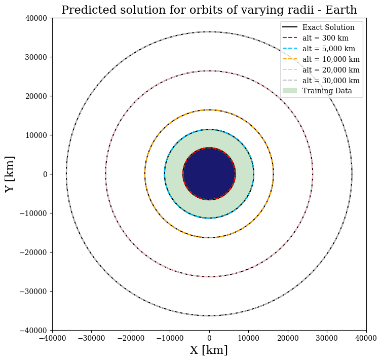
Figure 2: Koopman operator prediction and comparison against nonlinear dynamics of 5 orbits around Earth at various altitudes.

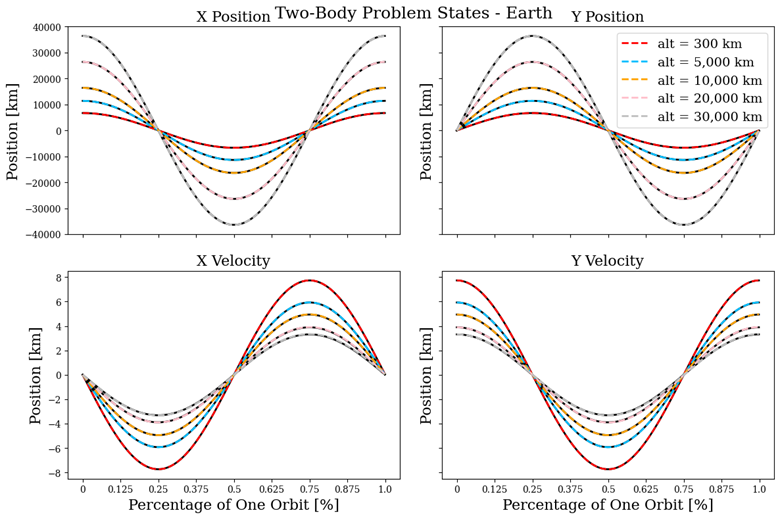
Figure 3: Four position and velocity states of the Earth orbits over one orbital period in comparison to the full nonlinear dynamics.

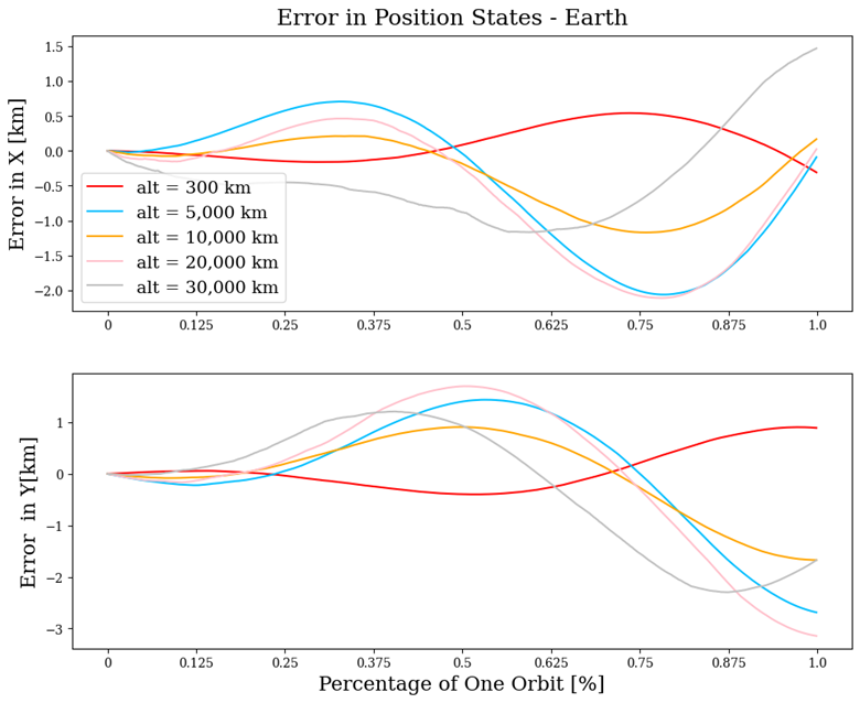
Figure 4: Error in position states over one orbital period for Earth.

The Koopman operator, although excellent at predicting learned nonlinear dynamics, can often struggle when generalized and implemented in other systems. Here, we show that the model proposed in this work generalizes quite accurately to two other 2BP’s of varying sizes. In particular, orbital trajectories around the Moon (for a smaller central body) and Jupiter (for a larger central body) were predicted using the the same Koopman operator learned from the dataset based on Earth’s orbit. As seen in Figures 7 and 8, the error in both the Moon’s and Jupiter’s orbits are slightly higher than that of the Earth’s, but the prediction still is highly effective. Figures 7 and 6 display the prediction of orbits for the previously mentioned set of $5$ different altitudes.

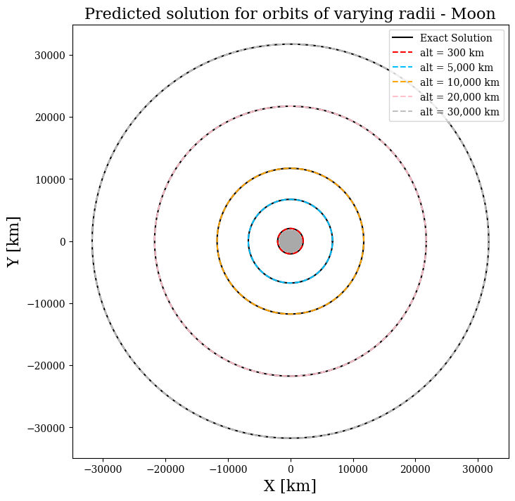
Figure 5: Koopman operator prediction and comparison against nonlinear dynamics of 5 orbits around the Moon at various altitudes.

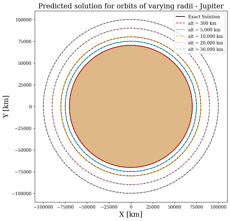
Figure 6: Koopman operator prediction and comparison against nonlinear dynamics of 5 orbits around Jupiter at various altitudes.

Plots of the error in the position state for both the Moon- and Jupiter-centered orbits allow us to analyse the effect of the size of the central body on the models ability to evolve the dynamics. A larger central body appears to have a greater periodic prediction error as compared to a central body that is smaller than that of the body the training data was derived from. As such, the possibility for the model to be used as a baseline, with additional data from the applied system added online, could enhance the performance of the model. With a short training time of around 80 min, it is not unreasonable to engage in the possibility of online data collection and learning to further enhance the accuracy of the predicted orbit.

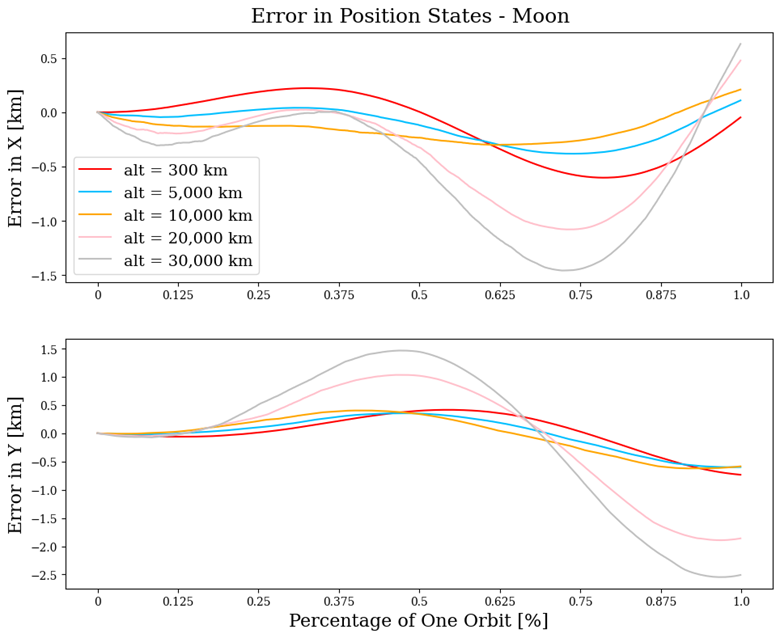
Figure 7: Error in position states over one orbital period for the Moon.

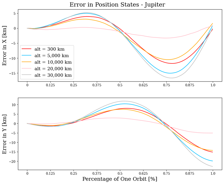
Figure 8: Error in position states over one orbital period for Jupiter.

5.2.2 Accuracy Metrics

We now look at the metrics provided in Section 4.1, and how the proposed Koopman operator is able to adhere to the conservative properties aforementioned. We see in Figure 9 that the values of all four metrics for the model around Earth are substantially low and very close to zero, hence illustrating the absolute error in each metric along the orbit is near zero. Furthermore, when these metrics are checked on orbits around both the Moon and Jupiter, Figures 10 and 11, the conservation of the invariant properties is also preserved, as the values are near zero. These metrics prove the accuracy and reliability of our model in representing the 2BP not only insofar as its specific trained dataset is concerned, but also in its generalized applications to other systems.

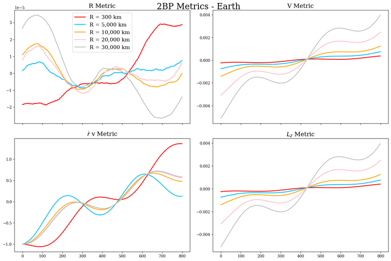
Figure 9: Invariant property metrics for the 2BP linearization around Earth.

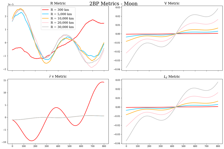
Figure 10: Invariant property metrics for the 2BP linearization around the Moon.

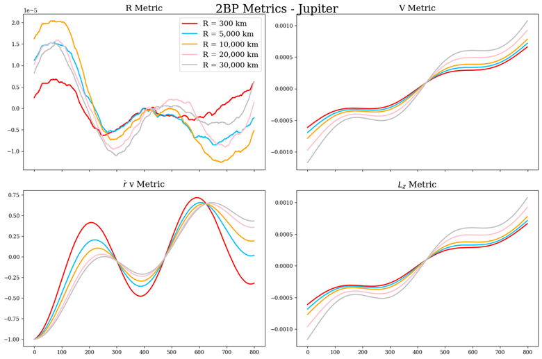
Figure 11: Invariant property metrics for the 2BP linearization around Jupiter.

5.2.3 Circular Restricted Three-Body Problem Linearization

The hyperparameters of the DNN used for all experiments with the CR3BP are outlined in Table 2. The total training time for the DNN used in the CR3BP model was 55 hours on an NVIDIA GeForce RTX 3090 GPU, which is substantially longer than that of the 2BP due to its highly increased lifted space and dataset size. However, it is important to note that this training can occur offline prior to the models use and would not be an issue in the online deployment of the model.

CR3BP Neural Network Hyperparameters
Hyperparameter	Value
Lifted Space Size	100
Hidden Layers	13
Neurons per hidden layer	105
Batch Size	16
Learning Rate	0.000001
Optimizer	Adam
Activation Function	SELU
Weight Decay	0.00001
Epochs	35000
$\gamma$	2
$\beta$	1
$\lambda_{L_{1}}$	0.004
$\lambda_{L_{2}}$	0.001
K matrix dimension	106 x 106

Table 2: Hyperparameters for CR3BP Neural Network

Figure 12 shows the linearized evolution of the dynamics that is generated by our Koopman operator. It shows that the DNN is able to learn appropriate observables and lift the dimension of the states such that the K matrix was able to accurately predict the orbit of the CR3BP by rendering it as a linear system. Because the orbit, like the 2BP, is in-plane, the $z$-axis position and velocity are zero, therefore we are able to plot the propagation of the dynamics on a 2D plane to further inspect the accuracy of the propagation, as done in Figure 13. Note that in both Figures 12 and 13 the scale of the Earth and Moon representations are chosen for ease of viewing, and are not to scale with the propagated orbit. We also show the evolution of each of the 4 states independently in Figure 14, comparing them to the nonlinear dynamics, to emphasise the ability to closely follow the intricate dynamics of the CR3BP. It shall be noted that although the CR3BP is propagated in the non-dimensionalized units, in these figures the dimensionalized units are restored, and are displayed in the rotating frame.

The initial condition for the orbit displayed in the aforementioned results was randomly selected from the test data set provided in the generated data set, in order to ensure it is not an IC that the DNN has seen before. The state vector is given as:

$$\mathbf{x_{0}}=\begin{bmatrix}0.8673\\ 0\\ 0\\ 0\\ -0.2546\\ 0\end{bmatrix}$$

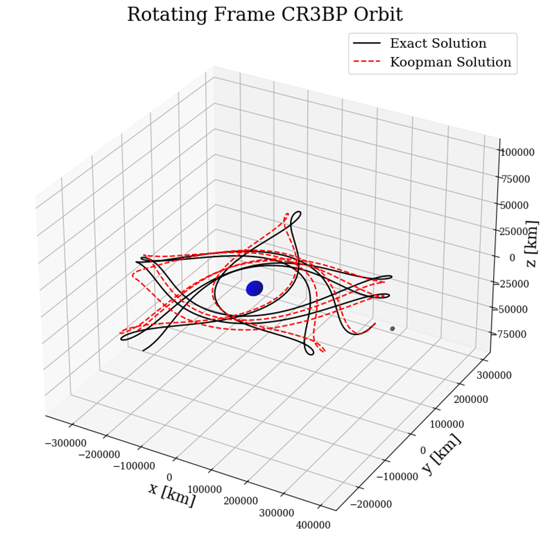
Figure 12: Orbital propagation of the Koopman model and nonlinear dynamics viewed in a 3D plot.

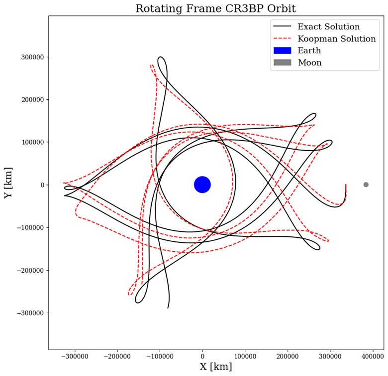
Figure 13: Orbital propagation of the Koopman model and nonlinear dynamics viewed in the 2D orbital plane.

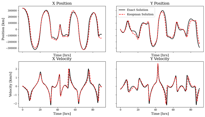
Figure 14: The four states of the CR3BP orbit, with the Koopman model compared to the nonlinear dynamics.

5.2.4 Accuracy Metrics

As mentioned in Section 4.2, the metric to determine the accuracy of our linear model is the Jacobi Constant. In order to display this metric, it has been calculated for both the nonlinear and linear models and then plotted against each other. The higher the accuracy of the linear model, the closer the linear Jacobi constant will follow that of the nonlinear dynamics. Figure 15 compares the constant of our model against that of the true, nonlinear dynamics, exhibiting a fair degree of accuracy in light of the complexity of the CR3BP.

Figure 15: The Jacobi Constant at every time instance for both the nonlinear and linear dynamics.

5.3 Training Loss

In this section we analyze the training loss for both models. We can see that from both Figures 16 and 17, the loss function exponentially decays as the number of training epochs increases. This is very typical behaviour of a NN model, and shows that the model is adequately trained for each prediction due to its steady state value reached. With more training, tuning of the hyperparameters and loss function it could be reduced even further.

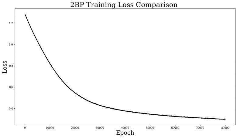
Figure 16: Neural Network training loss across all training epochs for the 2BP.

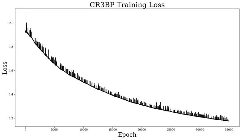
Figure 17: Neural Network training loss across all training epochs for the CR3BP.

5.4 Discussion

The propagation of the 2BP in the Earth system is very accurate, with minimal error in both the position states and metrics, even for IC’s that were outside of the trained region. The largest absolute error in all of the trialed IC’s in the Earth system was 3 km, which for that orbit translates to an error percentage of 0.01%. This percentage is calculated as the ratio of the largest error over the mean radius of the orbit.

By utilizing the LTI Koopman operator learned on the Earth system on the Moon and Jupiter systems, we see that there is a capability for the model to generalize to other dynamical systems, but the model is sensitive to variations in parameters in the nonlinear dynamics. The error in the predictions varied in comparison to the Earth model because of the dissimilar mass of the central body, ultimately changing its gravitational parameter. The largest error percentage in the Moon system was $\sim 0.008\%$ whilst the largest error in the Jupiter system was $\sim 0.02\%$. Although the errors are still very small, if such a system was to be used in a controls application or a trajectory tracking situation, these errors would have to be reduced further, or have the control system correct it.

The analysis of the accuracy of the 2BP Koopman model with the metrics in Section 4.1 shows that our model not only is able to predict the current trajectory of the orbit, but also is able to conserve the physical properties that are evident in the nonlinear dynamics. The learned linear model is even able to conserve these invariants for systems it has never seen before or been trained on, emphasising the remarkable capabilities of the Koopman operator to effectively linearize a nonlinear system, whilst remaining physically and mathematically valid. Likewise the analysis of the Jacobi Constant for the CR3BP model highlights its ability to conserve the physical properties related with its dynamics. Although the accuracy of the CR3BP LTI model is not as high as the 2BP model, it clearly illustrates the ability to capture key important features, with the relative error in the Jacobi Constant being $\lesssim 12.7\%$. Both the 2BP and CR3BP cases show that the model is accurately learning the dynamics in the linearization and not simply learning shapes or curves.

Although the 2BP shows excellent results and accuracy in the linear model, the CR3BP apparently still exhibits a higher relative error in its prediction that could be subsequently improved on. The model clearly learns the dynamics of the nonlinear system, but further fine tuning in the loss function, training, hyperparameters or data would be necessary to improve the results to the point that it may be used in a real life problem.

It is important to note that the linear models presented in this work are LTI, and hence transform the complex nonlinear dynamics into the simple, well-understood form that is the LTI system. Hence, it is possible to employ a wide variety of techniques such as proving stability, observability and controllability that are commonly used by engineers in guidance, navigation, and control.

6 CONCLUSION

The advancements in this paper are significant because, to our knowledge, this is the first time that both the 2BP and CR3BP have been globally linearized. Our proposed model, which is also capable of generalization to a wide array of celestial systems, demonstrates a fast and accurate method for developing a linear Koopman operator representation of the 2BP and CR3BP. We establish the accuracy of both models through analysis of the invariant properties of each nonlinear system, and show that they hold for our linearized model.

The LTI models discovered in this paper offer a novel opportunity for several advancements in the control and estimation of two- and three-body problems. The models have diverse applications that can replace a number of older methods such as the CW equations, Taylor series linearization, Kalman filtering and system ID.

7 FUTURE WORK

Investigations of the capacity to generalize the Koopman operator to various orbits and resolve the effects of the gravitational parameter on its predictions is an immediate area of improvement in this model. Furthermore, the work with the CR3BP model suggests that the Koopman operator is reasonably capable of learning complex dynamics. Hence, a realistic two-body model, such as one including drag, solar radiation pressure and a more precise gravitational potential of the Earth (e.g., J2 gravitational parameter), would allow for a real-world application of this Koopman operator.

The hyperparameters of the DNN in this work could be further explored, as many of them were empirically chosen and adjust until the final parameters were chosen. Increasing the number of neurons and hidden layers may allow for improved prediction. An investigation into whether it is more important to have a higher latent space or higher number of hidden layers or both, would be relevant in addressing the larger error of the CR3BP and how that aspect may be mitigated.

For implementing practical applications of the framework, the Koopman model should be expanded with EDMDc [49] (i.e., EDMD with control) in order to learn the control matrix required for a real-world control application of the linearized dynamics. It is worth noting that accurate state and control data should be paired when learning the model based on EDMDc.

[]George Nehma received B.Sc degree in Aerospace Engineering from Florida Institute of Technology, USA in 2020. He is currently pursuing M.S. and PhD in Aerospace at Florida Institute of Technology, USA. His research interests include deep learning of Koopman Operator theory and applications onto space systems and vehicles.

[]Dr. Madhur Tiwari is the Director of the Autonomy Lab and Assistant Professor of Aerospace Engineering at Florida Institute of Technology. He specializes in robotics, machine learning and control for aerospace systems. Currently, he is teaching Spaceflight Mechanics and Modern Control Theory at Florida Institute of Technology.

[]Dr. Manasvi Lingam is an Assistant Professor in Aerospace, Physics, and Space Sciences at Florida Institute of Technology. His research interests in aerospace encompass encompass mission design (with a focus on enabling life detection), propulsion systems (e.g., light sails), and astrodynamics.

References

- [1] S. J. Aarseth Gravitational N-Body Simulations. Cambridge: Cambridge University Press, 2003.
- [2] A. Arsie and N. A. Balabanova Collision trajectories and regularisation of two-body problem on s2 Journal of Geometry and Physics, vol. 191, p. 104883, 2023. [Online]. Available: https://www.sciencedirect.com/science/article/pii/S0393044023001353
- [3] S. Alhowaity Computational algorithm to solve two–body problem using power series in geocentric system Applied Mathematics and Nonlinear Sciences, vol. 8, no. 2, pp. 39–46, 2023. [Online]. Available: https://doi.org/10.2478/amns.2021.2.00300
- [4] E. I. Abouelmagd, J. L. García Guirao, and J. Llibre On the periodic orbits of the perturbed two- and three-body problems Galaxies, vol. 11, no. 2, p. 58, 2023, copyright - © 2023 by the authors. Licensee MDPI, Basel, Switzerland. This article is an open access article distributed under the terms and conditions of the Creative Commons Attribution (CC BY) license (https://creativecommons.org/licenses/by/4.0/). Notwithstanding the ProQuest Terms and Conditions, you may use this content in accordance with the terms of the License; Last updated - 2023-11-24. [Online]. Available: https://www.mdpi.com/2075-4434/11/2/58
- [5] V. Szebehely Theory of Orbit: The Restricted Problem of Three Bodies. New York, NY: Academic Press, 1967.
- [6] J. Barrow-Green Poincaré and the three body problem. Providence, RI: AMS, 1997.
- [7] C. Marchal The three-body problem, ser. Studies in Astronautics. Amsterdam, Netherlands: Elsevier, 1990, no. 4.
- [8] M. C. Gutzwiller Moon-Earth-Sun: The oldest three-body problem Rev. Mod. Phys., vol. 70, no. 2, pp. 589–639, Apr. 1998.
- [9] C. D. Murray and S. F. Dermott Solar System Dynamics. Cambridge, UK: Cambridge Univ. Press, 1999.
- [10] M. Valtonen and H. Karttunen The Three-Body Problem. Cambridge, UK: Cambridge Univ. Press, 2005.
- [11] M. Valtonen, J. Anosova, K. Kholshevnikov, A. Mylläri, V. Orlov, and K. Tanikawa The Three-body Problem from Pythagoras to Hawking. Cham, CH: Springer International Publishing, 2016.
- [12] P. M. Pires, C. F. de Melo, M. C. F. P. S. Zanardi, and S. M. G. Winter Celestial mechanics: new discoveries and challenges for space exploration. The European Physical Journal Special Topics, vol. 232, no. 18-19, pp. 2881 – 2887, 2023. [Online]. Available: https://link.springer.com/article/10.1140/epjs/s11734-023-01074-2
- [13] K. F. Wakker Fundamentals of Astrodynamics. Delft, NL: Institutional Repository Library, 2015.
- [14] W. H. CLOHESSY and R. S. WILTSHIRE Terminal guidance system for satellite rendezvous. Journal of the Aerospace Sciences, vol. 27, no. 9, pp. 653 – 658, 1960. [Online]. Available: https://arc.aiaa.org/doi/abs/10.2514/8.8704
- [15] P. Luke T. and S. Daniel J. Local orbital elements for the circular restricted three-body problem. Journal of Guidance, Control, and Dynamics, vol. 46, no. 12, pp. 2275 – 2289, 2023. [Online]. Available: https://arc.aiaa.org/doi/10.2514/1.G007435
- [16] V. V. Makarov Why is the moon synchronously rotating ? Monthly Notices of the Royal Astronomical Society, vol. 434, pp. L21–L25, Jul. 2013.
- [17] B. O. Koopman Hamiltonian systems and transformation in hilbert space Proceedings of the National Academy of Sciences, vol. 17, no. 5, pp. 315–318, 1931. [Online]. Available: https://www.pnas.org/doi/abs/10.1073/pnas.17.5.315
- [18] M. O. Williams, I. G. Kevrekidis, and C. W. Rowley A data–driven approximation of the koopman operator: Extending dynamic mode decomposition Journal of Nonlinear Science, vol. 25, no. 6, p. 1307–1346, Jun. 2015. [Online]. Available: http://dx.doi.org/10.1007/s00332-015-9258-5
- [19] S. L. Brunton, M. Budišić, E. Kaiser, and J. N. Kutz Modern koopman theory for dynamical systems SIAM Review, vol. 64, no. 2, 2022.
- [20] E. Kaiser, J. N. Kutz, and S. L. Brunton Data-driven discovery of koopman eigenfunctions for control Machine Learning: Science and Technology, vol. 2, no. 3, p. 035023, 2021.
- [21] Y. LeCun, Y. Bengio, and G. Hinton Deep learning nature, vol. 521, no. 7553, pp. 436–444, 2015.
- [22] B. Lusch, J. N. Kutz, and S. L. Brunton Deep learning for universal linear embeddings of nonlinear dynamics Nature Communications, vol. 9, no. 1, Nov 2018. [Online]. Available: https://doi.org/10.1038%2Fs41467-018-07210-0
- [23] G. Cybenko Approximation by superpositions of a sigmoidal function Mathematics of control, signals and systems, vol. 2, no. 4, pp. 303–314, 1989.
- [24] K. Hornik, M. Stinchcombe, and H. White Universal approximation of an unknown mapping and its derivatives using multilayer feedforward networks Neural networks, vol. 3, no. 5, pp. 551–560, 1990.
- [25] K. Hornik, M. Stinchcombe, and H. White Multilayer feedforward networks are universal approximators Neural networks, vol. 2, no. 5, pp. 359–366, 1989.
- [26] P. Amaro-Seoane et al. Laser interferometer space antenna 2017.
- [27] P. Amaro-Seoane et al. Astrophysics with the Laser Interferometer Space Antenna Living Reviews in Relativity, vol. 26, no. 1, p. 2, Dec. 2023.
- [28] M. Tiwari, G. Nehma, and B. Lusch Computationally efficient data-driven discovery and linear representation of nonlinear systems for control IEEE Control Systems Letters, vol. 7, pp. 3373–3378, 2023.
- [29] G. Snyder and Z. Song Koopman operator theory for nonlinear dynamic modeling using dynamic mode decomposition 2021.
- [30] P. J. SCHMID Dynamic mode decomposition of numerical and experimental data Journal of Fluid Mechanics, vol. 656, p. 5–28, 2010.
- [31] S. Klus and C. Schütte Towards tensor-based methods for the numerical approximation of the perron–frobenius and koopman operator Journal of Computational Dynamics, vol. 3, no. 2, pp. 139–161, 2016.
- [32] S. Brunton, B. Brunton, J. Proctor, and J. Kutz Koopman observable subspaces and finite linear representations of nonlinear dynamical systems for control PloS one, vol. 11, 10 2015.
- [33] C. Folkestad, D. Pastor, I. Mezic, R. Mohr, M. Fonoberova, and J. Burdick Extended dynamic mode decomposition with learned koopman eigenfunctions for prediction and control 2020.
- [34] M. Svec, S. Iles, and J. Matusko Predictive direct yaw moment control based on the koopman operator. IEEE Transactions on Control Systems Technology, Control Systems Technology, IEEE Transactions on, IEEE Trans. Contr. Syst. Technol, vol. 31, no. 6, pp. 2912 – 2919, 2023. [Online]. Available: https://portal.lib.fit.edu/login?url=https://search.ebscohost.com/login.aspx?direct=true&db=edseee&AN=edseee.10122214&site=eds-live
- [35] V. Zinage and E. Bakolas Neural koopman lyapunov control Neurocomputing, vol. 527, pp. 174–183, Mar. 2023. [Online]. Available: https://www.sciencedirect.com/science/article/pii/S0925231223000413
- [36] R. Penrose A generalized inverse for matrices Mathematical Proceedings of the Cambridge Philosophical Society, vol. 51, no. 3, p. 406–413, 1955.
- [37] A. Junker, J. Timmermann, and A. Trachtler Data-driven models for control engineering applications using the koopman operator In 2022 3rd International Conference on Artificial Intelligence, Robotics and Control (AIRC). IEEE, May 2022. [Online]. Available: https://doi.org/10.1109%2Fairc56195.2022.9836980
- [38] M. Korda and I. Mezić Linear predictors for nonlinear dynamical systems: Koopman operator meets model predictive control Automatica, vol. 93, pp. 149–160, Jul 2018. [Online]. Available: https://doi.org/10.1016%2Fj.automatica.2018.03.046
- [39] A. Allahvirdi-Zadeh, K. Wang, and A. El-Mowafy Precise orbit determination of leo satellites based on undifferenced gnss observations Journal of Surveying Engineering, vol. 148, no. 1, p. 03121001, 2022. [Online]. Available: https://ascelibrary.org/doi/abs/10.1061/%28ASCE%29SU.1943-5428.0000382
- [40] L. Ye, C. Liu, F. Liu, W. Zhang, and H. Baoyin The low fuel consumption keeping method of eccentricity under integrated keeping of inclination-longitude Aerospace, vol. 10, no. 2, 2023. [Online]. Available: https://www.mdpi.com/2226-4310/10/2/135
- [41] D. Vallado and W. McClain Fundamentals of Astrodynamics and Applications, ser. College custom series. McGraw-Hill Companies, Incorporated, 1997. [Online]. Available: https://books.google.com/books?id=pGqFPwAACAAJ
- [42] G. Franzini and M. Innocenti Relative motion dynamics in the restricted three-body problem Journal of Spacecraft and Rockets, vol. 56, no. 5, pp. 1322–1337, 2019. [Online]. Available: https://doi.org/10.2514/1.A34390
- [43] A. Y. Ng Feature selection, l1 vs. l2 regularization, and rotational invariance In Proceedings of the Twenty-First International Conference on Machine Learning, ser. ICML ’04. New York, NY, USA: Association for Computing Machinery, 2004, p. 78. [Online]. Available: https://doi.org/10.1145/1015330.1015435
- [44] D. Batic, M. Nowakowski, and A. M. Abdelhaq New vistas on the Laplace-Runge-Lenz vector Reviews in Physics, vol. 10, p. 100084, Jun. 2023.
- [45] A. P. Wilmer and R. A. Bettinger Lagrangian dynamics and the discovery of cislunar periodic orbits. Nonlinear Dynamics: An International Journal of Nonlinear Dynamics and Chaos in Engineering Systems, vol. 111, no. 1, pp. 155 – 178, 2023. [Online]. Available: https://portal.lib.fit.edu/login?url=https://search.ebscohost.com/login.aspx?direct=true&db=edssjs&AN=edssjs.98923734&site=eds-live
- [46] L. Meirovitch Methods of Analytical Dynamics, ser. Advanced engineering series. McGraw-Hill, 1970. [Online]. Available: https://books.google.com/books?id=GlV5ywEACAAJ
- [47] R. Battin An Introduction to the Mathematics and Methods of Astrodynamics, ser. AIAA Education Series. American Institute of Aeronautics & Astronautics, 1999. [Online]. Available: https://books.google.com/books?id=OjH7aVhiGdcC
- [48] J. A. Riousset and M. Lingam Jacobi integral: A real-world application of the Lagrangian formulation arXiv e-prints, p. arXiv:2312.15800, Dec. 2023.
- [49] C. Folkestad, D. Pastor, I. Mezic, R. Mohr, M. Fonoberova, and J. Burdick Extended dynamic mode decomposition with learned koopman eigenfunctions for prediction and control In 2020 american control conference (acc). IEEE, 2020, pp. 3906–3913.
[![[Uncaptioned image]](/html/2403.08965/assets/Images/nehma.jpeg) ]George Nehma
received B.Sc degree in Aerospace Engineering from Florida Institute of Technology, USA in 2020. He is currently pursuing M.S. and PhD in Aerospace at Florida Institute of Technology, USA. His research interests include deep learning of Koopman Operator theory and applications onto space systems and vehicles.