Towards Efficient Risk-Sensitive Policy Gradient: An Iteration Complexity Analysis

Abstract

Reinforcement Learning (RL) has shown exceptional performance across various applications, enabling autonomous agents to learn optimal policies through interaction with their environments. However, traditional RL frameworks often face challenges in terms of iteration complexity and robustness. Risk-sensitive RL, which balances expected return and risk, has been explored for its potential to yield probabilistically robust policies, yet its iteration complexity analysis remains underexplored. In this study, we conduct a thorough iteration complexity analysis for the risk-sensitive policy gradient method, focusing on the REINFORCE algorithm and employing the exponential utility function. We obtain an iteration complexity of ${\mathcal{O}}(\epsilon^{-2})$ to reach an $\epsilon$-approximate first-order stationary point (FOSP). We investigate whether risk-sensitive algorithms can achieve better iteration complexity compared to their risk-neutral counterparts. Our theoretical analysis demonstrates that risk-sensitive REINFORCE can have a reduced number of iterations required for convergence. This leads to improved iteration complexity, as employing the exponential utility does not entail additional computation per iteration. We characterize the conditions under which risk-sensitive algorithms can achieve better iteration complexity. Our simulation results also validate that risk-averse cases can converge and stabilize more quickly after approximately half of the episodes compared to their risk-neutral counterparts.

1 Introduction

Reinforcement Learning (RL) is the problem of learning optimal policies through interactions with an environment (Sutton et al., 1999; Kaelbling et al., 1996). RL has shown remarkable success in a wide range of applications, e.g., board and video game playing (Silver et al., 2016; Mnih et al., 2013). However, it is widely acknowledged that classical RL is both lacking in robustness and falls short in terms of iteration efficiency (Casper et al., 2023; AlMahamid & Grolinger, 2021). One reason is that standard RL only takes expected return into consideration.

Risk-Sensitive RL algorithms (Mihatsch & Neuneier, 2002; Shen et al., 2014; Berkenkamp et al., 2017) mitigate these issues by taking into account not only the expected value of performance but also its variability. This allows for adjusting the balance between the expected return and variability. Consideration of risk is crucial in high-stake and safety critical applications, such as finance (Filos, 2019; Charpentier et al., 2021), autonomous driving (Zhang et al., 2021) and robotics (Majumdar et al., 2017). Various risk measures, such as Conditional Value-at-Risk (CVaR) (Qiu et al., 2021; Prashanth et al., 2022), Optimized Certainty Equivalents (OCE) (Lee et al., 2020) and exponential utility function (Mihatsch & Neuneier, 2002; Fei et al., 2020; Eriksson & Dimitrakakis, 2019; Prashanth et al., 2022; Noorani & Baras, 2021), have been used to incorporate risk into RL algorithms. The robustness of the policies obtained using risk-sensitive RL algorithms that use exponential utility function has been proven analytically and has been shown experimentally, e.g., see Noorani et al. (2022).

While previous work has derived risk-sensitive RL algorithms based on these risk measures, their iteration complexity has received limited attention. Nevertheless, understanding iteration complexity (Kakade, 2003; Dann & Brunskill, 2015; Lattimore et al., 2013) can provide theoretical insights into risk-sensitive RL and guide the development of more efficient algorithms. Here, we focus on the issue of iteration complexity of risk-sensitive RL algorithms. This motivates our primary question:

Do risk-sensitive algorithms exhibit improved iteration complexity over standard algorithms?

To address our primary question regarding iteration complexity, we focus on the policy gradient (PG) method REINFORCE (Williams, 1992; Sutton et al., 1999; Baxter & Bartlett, 2001) and its risk-sensitive counterpart (Noorani & Baras, 2021), which employs the exponential utility.

Previous studies have examined the iteration complexity of the standard risk-neutral REINFORCE algorithm, but few have explored the iteration complexity of the risk-sensitive REINFORCE as we mentioned. Papini et al. (2018) introduced the stochastic variance-reduced policy gradient (SVRPG) method, which requires ${\mathcal{O}}(\epsilon^{-2})$ iterations to achieve $\left\|\nabla J(\theta)\right\|\leq\epsilon$. Xu et al. (2020) provided an improved convergence analysis of SVRPG and show an iteration complexity of ${\mathcal{O}}(\epsilon^{-\frac{5}{3}})$ to achieve an $\epsilon$-approximate first-order stationary point (FOSP). Subsequently, Xu et al. (2019) proposed a SRVRPG algorithm that improves this iteration complexity to ${\mathcal{O}}(\epsilon^{-\frac{3}{2}})$. Papini (2021) proved the ${\mathcal{O}}(\epsilon^{-2})$ iteration complexity for REINFORCE. Yuan et al. (2022) achieved an ${\mathcal{O}}(\epsilon^{-2})$ iteration complexity for the exact gradient of the REINFORCE algorithm aimed at reaching a FOSP.

Reference	Type	Guarantee	Bound
Papini et al. (2018)	RN	FOSP	${\mathcal{O}}(\epsilon^{-2})$
Xu et al. (2020)	RN	FOSP	${\mathcal{O}}(\epsilon^{-\frac{5}{3}})$
Xu et al. (2019)	RN	FOSP	${\mathcal{O}}(\epsilon^{-\frac{3}{2}})$
Papini (2021)	RN	FOSP	${\mathcal{O}}(\epsilon^{-2})$
Yuan et al. (2022)	RN	FOSP	${\mathcal{O}}(\epsilon^{-2})$
Ours	RS	FOSP	${\mathcal{O}}(\epsilon^{-2})$

Table 1: Iteration complexity results of previous standard REINFORCE and our risk-sensitive REINFORCE. RN denotes risk-neutral and RS denotes risk-sensitive.

In this study, we analyze the iteration complexity of the risk-sensitive REINFORCE under a most general assumption of bounding the second moment of the gradient. This analysis is the first of its kind. We present in Table 1 iteration complexity results from some previous studies on standard risk-neutral REINFORCE and our risk-sensitive REINFORCE. Remarkably, we not only provide insights into the iteration complexity of risk-sensitive REINFORCE but also draw a comparison with the standard risk-neutral REINFORCE, which serves as the baseline. Our analysis reveals that the risk-sensitive algorithm can achieve convergence with a reduced number of iterations under certain risk-sensitive parameters. Overall, we contribute in three key aspects and we discuss these contributions in detail here:

Iteration complexity analysis for risk-sensitive REINFORCE

We first conduct a comprehensive analysis of the iteration complexity for the risk-sensitive REINFORCE algorithm, which exhibits an iteration complexity of ${\mathcal{O}}(\epsilon^{-2})$. This analysis aims to achieve an $\epsilon$-approximate first-order stationary point (FOSP) such that $\mathbb{E}\left[\left\|\nabla J_{\beta}(\theta)\right\|\right]\leq\epsilon$, where $J_{\beta}$ is the risk-sensitive value function parameterized by $\theta$ with a risk-sensitive parameter $\beta$. Our analysis builds on an expected smoothness assumption introduced by Khaled & Richtárik (2020), as shown in Assumption 2. This assumption bounds the second moment of the gradient and serves as the most general assumption for modeling it.

Notably, Yuan et al. (2022) successfully derived convergence rates and iteration complexity results for the standard risk-neutral REINFORCE algorithm, relying on the this assumption, which they referred to as the ABC assumption. However, they did not examine the risk-sensitive REINFORCE algorithm. They suggested that an interesting avenue of investigation would be to determine whether the analysis based on the ABC assumption can be extended to other domains or algorithms. To the best of our knowledge, this is the first instance of such an extension, adding a novel perspective to the field of risk-sensitive reinforcement learning.

Iteration complexity comparison between risk-sensitive and risk-neutral REINFORCE

We formally compare the iteration complexity of risk-sensitive and risk-neutral REINFORCE. Both algorithms exhibit iteration complexities of ${\mathcal{O}}(\epsilon^{-2})$, guaranteed by a FOSP, However, when the risk-sensitive parameter $\beta$ is chosen appropriately, we can achieve a reduced number of iterations required for convergence for the risk-sensitive algorithm compared to the risk-neutral one. We quantify such $\beta$ values in Theorem 2.

Simulation results

We conduct numerical experiments using the Minigrid navigation environment, employing the risk-neutral REINFORCE algorithm as a baseline for comparison. The risk-averse cases stabilize after approximately half of the episodes compared to the risk-neutral case. These results confirm our theoretical findings that risk-sensitive REINFORCE can exhibit better iteration complexity than the standard risk-neutral REINFORCE.

2 Preliminaries

Consider an optimization problem (Jain et al., 2017) defined as:

$$\min_{\theta\in\mathbb{R}^{d}}J(\theta),$$ (1)

where the function $J(\theta)$ is the expected return parameterized by $\theta$ and is assumed to be Lipschitz smooth, as in Assumption 1.

Assumption 1 (Lipschitz Smoothness).

There exists $L\in\mathbb{R}^{+}$ such that, for all $\theta,\theta^{\prime}\in{\mathbb{R}}^{d}$, we have

$$\left\|\nabla J(\theta)-\nabla J(\theta^{\prime})\right\|\leq L\left\|\theta-\theta^{\prime}\right\|.$$ (2)

The gradient descent for solving the optimization problem 1 gives the following iteration:

$$\theta_{t+1}=\theta_{t}-\eta_{t}\nabla J(\theta_{t}),$$ (3)

where $\eta_{t}$ is the step size.

Based on Assumption 1,

$$J(\theta^{\prime})\leq J(\theta)+\nabla J(\theta)(\theta^{\prime}-\theta)^{\top}+\frac{L}{2}\left\|\theta^{\prime}-\theta\right\|^{2}.$$ (4)

Let’s define $g(\theta^{\prime})=J(\theta)+\nabla J(\theta)(\theta^{\prime}-\theta)^{\top}+\frac{L}{2}\left\|\theta^{\prime}-\theta\right\|^{2}$, then make the gradient of $g(\theta^{\prime})=0$,

$$\nabla J(\theta)+L(\theta^{\prime}-\theta)=0,$$

$$\theta^{\prime*}=\theta-\frac{1}{L}\nabla J(\theta).$$ (5)

Then,

$$J(\theta^{\prime*})\leq g(\theta^{\prime*})=J(\theta)-\frac{1}{2L}\left\|\nabla J(\theta)\right\|^{2}.$$ (6)

With the step size $\eta_{t}=\frac{1}{L}$,

$$J(\theta_{t})-J(\theta_{t+1})\geq\frac{1}{2L}\left\|\nabla J(\theta_{t})\right\|^{2}.$$ (7)

Taking summation over $T+1$ steps,

$$J(\theta_{0})-J(\theta^{*})\geq J(\theta_{0})-J(\theta_{T})\geq\frac{1}{2L}\sum_{t=0}^{T}\left\|\nabla J(\theta_{t})\right\|^{2},$$ (8)

where $J(\theta^{*})$ is the global optimum value.

We have,

$$\min_{0\leq t\leq T}\left\|\nabla J(\theta_{t})\right\|^{2}\leq\frac{2L(J(\theta_{0})-J(\theta^{*}))}{T+1}.$$ (9)

Subsequently, we integrate risk into the framework by employing the exponential utility function (Mihatsch & Neuneier, 2002; Fei et al., 2020; Eriksson & Dimitrakakis, 2019; Liu et al., 2023; Prashanth et al., 2022; Noorani & Baras, 2021), transitioning from the standard risk-neutral objective $J$ to the risk-sensitive objective $J_{\beta}$, where $\beta$ is the risk-sensitivity parameter. By taking the Taylor expansion, as shown later in Equation 16, we consider not only the expected value but also the variance, thus incorporating risk into the framework. Now, it is worth noting that the risk-sensitive objective $J_{\beta}$ exhibits Lipschitz smoothness but with a different constant $L_{\beta}$ in our case, as proven in Appendix B.

Building upon the Lipschitz smoothness assmuption in Assumption 1, we introduce the following assumption, which bounds the second moment of the gradient, following the work by (Khaled & Richtárik, 2020).

Assumption 2 (Expected smoothenss (Khaled & Richtárik, 2020)).

There exists constants $A,B,C\in\mathbb{R}_{\geq 0}$ such that for all $\theta\in{\mathbb{R}}^{d}$, the policy gradient estimator satisfies

$$\mathbb{E}\left[\left\|\widehat{\nabla}J_{\beta}(\theta)\right\|^{2}\right]\leq 2A(J_{\beta}^{*}-J_{\beta}(\theta))+B\left\|\nabla J_{\beta}(\theta)\right\|^{2}+C.$$ (10)

After the preliminaries of smoothness assumption of value function and policy parameterization, we study policy gradient methods.

3 Policy Gradient Methods

In this section, we discuss policy gradient (PG) methods, including some preliminaries about the Markov Decision Process (MDP), the REINFORCE algorithm, and the risk-sensitive REINFORCE algorithm.

3.1 Markov Decision Process (MDP)

We examine a Markov Decision Process (MDP) characterized by the tuple $\{{\mathcal{S}},{\mathcal{A}},{\mathcal{P}},r,\gamma,\rho\}$. In this setup, ${\mathcal{S}}$ represents the state space, ${\mathcal{A}}$ is the action space, and ${\mathcal{P}}$ is the transition model. The transition model, denoted as ${\mathcal{P}}(s^{\prime}\mid s,a)$, signifies the probability of transitioning from state $s$ to $s^{\prime}$ when taking action $a$. The reward function, denoted as $r(s,a)$, produces bounded rewards in the range of $[r_{\min},r_{\max}]$ for state-action pairs $(s,a)$, with $r_{\max}$ being a positive constant.

The parameters $\gamma\in[0,1)$ and $\rho$ denote the discount factor and the initial state distribution, respectively. The agent’s behavior is captured through a policy $\pi$, which resides in the space of probability distributions over actions at each state. This is represented as $\pi(a\mid s)$.

We define the probability density $p(\tau\mid\pi)$ for a single trajectory $\tau$ being generated under policy $\pi$ as follows:

$$p(\tau\mid\pi)=\rho(s_{0})\prod_{t=0}^{\infty}\pi(a_{t}\mid s_{t}){\mathcal{P}}(s_{t+1}\mid s_{t},a_{t}).$$ (11)

Let ${\mathcal{R}}(\tau)=\vcentcolon\sum_{t=0}^{\infty}\gamma^{t}r(s_{t},a_{t})$ be the total discounted rewards accumulated along trajectory $\tau$. We define the risk-neutral expected return of $\pi$ as:

$$J(\pi)\stackrel{{\scriptstyle\text{def}}}{{=}}\mathbb{E}_{\tau\sim p(\cdot\mid\pi)}\left[{\mathcal{R}}(\tau)\right].$$ (12)

3.2 REINFORCE Algorithm

We consider stochastic and parameterized policies, represented as $\{\pi_{\theta}:\theta\in\mathbb{R}^{d}\}$, with the underlying assumption that these policies are differentiable concerning the parameter $\theta$. Let’s define $J(\pi_{\theta})$ as $J(\theta)$, and we can also express the probability of a trajectory given $\theta$ as $p(\tau\mid\pi_{\theta})=p(\tau\mid\theta)$.

Policy gradient (PG) methods utilize gradient ascent within the parameter space $\theta$, to identify the policy that maximizes the expected return. We denote the corresponding optimal expected return as $J^{*}\stackrel{{\scriptstyle\text{def}}}{{=}}J(\theta^{*})$.

The gradient $\nabla J(\theta)$ of the expected return is expressed as following:

$$\nabla J(\theta)=\int{\mathcal{R}}(\tau)\nabla p(\tau\mid\theta)d\tau\overset{\ref{eq:p}}{=}\mathbb{E}_{\tau}\left[\sum_{t=0}^{\infty}\nabla_{\theta}\log\pi_{\theta}(a_{t}\mid s_{t})\sum_{t^{\prime}=0}^{\infty}\gamma^{t^{\prime}}r(s_{t^{\prime}},a_{t^{\prime}})\right].$$ (13)

The REINFORCE gradient can be simplified by leveraging the fact that future actions do not depend on past rewards. This leads to the following formulation of the full gradient (Sutton & Barto, 2018):

$$\nabla J(\theta)=\mathbb{E}_{\tau}\left[\sum_{t=0}^{\infty}\nabla_{\theta}\log\pi_{\theta}(a_{t}|s_{t})\sum_{t^{\prime}=t}^{\infty}\gamma^{t^{\prime}}r(s_{t^{\prime}},a_{t^{\prime}})\right]=\mathbb{E}_{\tau}\left[\sum_{t=0}^{\infty}\nabla_{\theta}\log\pi_{\theta}(a_{t}|s_{t})R(t)\right],$$ (14)

where we define $\displaystyle R(t)\stackrel{{\scriptstyle\text{def}}}{{=}}\sum_{t^{\prime}=t}^{\infty}\gamma^{t^{\prime}}r(s_{t^{\prime}},a_{t^{\prime}})$ as the discounted rewards-to-go.

3.3 Risk-Sensitive REINFORCE Algorithm

After discussing the risk-neutral PG, we review the risk-sensitive PG, which is an extension of the traditional PG (Sutton et al., 1999; Kakade, 2001). In this extension, the objective is to optimize a policy by considering not only the expected return but also some measures of risk, such as conditional value-at-risk (CVaR) (Qiu et al., 2021; Prashanth et al., 2022), optimized certainty equivalents (OCE) (Lee et al., 2020) and exponential utility function (Mihatsch & Neuneier, 2002; Fei et al., 2020; Eriksson & Dimitrakakis, 2019; Prashanth et al., 2022; Noorani & Baras, 2021).

In this work, we employ the exponential utility function to incorporate risk into the system’s performance measure due to its computation convenience and mathematical tractability. The risk-sensitive REINFORCE algorithm aims to maximize the following objective:

$$J_{\beta}(\pi)=\vcentcolon\mathbb{E}_{\tau\sim p(\cdot\mid\pi)}\left[\beta e^{\beta{\mathcal{R}}(\tau)}\right],$$ (15)

where $J_{\beta}(\pi)$ is the risk-sensitive objective following a policy $\pi$ and satisfies the Lipschitz smoothness in Assumption 1, $\beta\neq 0$ represents the risk-sensitivity parameter, ${\mathcal{R}}(\tau)$ denotes the cumulative discounted rewards along a trajectory $\tau$ as in Section 3.1.

Some previous work (Fei et al., 2020; Hau et al., 2023) utilized the objective of the entropic risk measure, defined as $\frac{1}{\beta}\log\big{(}\mathbb{E}_{\tau\sim p(\cdot\mid\pi)}\left[e^{\beta{\mathcal{R}}(\tau)}\right]\big{)}$. From an optimization perspective, this objective shares the same optimal policy as our objective $J_{\beta}(\pi)$, as they have the same argmax. The optimal policy is derived as $\pi^{*}=\arg\max_{\pi}J_{\beta}(\pi)$. By taking a Taylor expansion of the risk-sensitive objective:

$$\mathbb{E}\left[\beta e^{\beta{\mathcal{R}}(\tau)}\right]=\beta+\beta^{2}\mathbb{E}\left[{\mathcal{R}}(\tau)\right]+\frac{\beta^{3}}{2}\mathbb{E}\left[{\mathcal{R}}^{2}(\tau)\right]+{\mathcal{O}}(\beta^{4}).$$ (16)

In cases where $\beta$ is negative (reflecting risk-averse behavior), maximizing $J_{\beta}(\pi)$ is equivalent to simultaneously maximizing the expected return and minimizing the variance of the return, which helps stabilize learning. Conversely, when $\beta$ is positive (indicating risk-seeking behavior), maximizing $J_{\beta}(\pi)$ becomes equivalent to maximizing both the expected return and the variance of the return.

We aim to explore whether adjusting the risk-sensitivity parameter can potentially reduce iteration complexity for risk-averse REINFORCE compared to risk-neutral REINFORCE. Achieving this would be highly beneficial as it would allow for both robustness and faster convergence simultaneously.

The gradient of the objective for the risk-sensitive REINFORCE is expressed as following:

$$\nabla J_{\beta}(\theta) =\mathbb{E}_{\tau}\left[\sum_{t=0}^{\infty}\nabla_{\theta}\log\pi_{\theta}(a_{t}\mid s_{t})\cdot\beta e^{\beta\sum_{t^{\prime}=t}^{\infty}\gamma^{t^{\prime}}r(s_{t^{\prime}},a_{t^{\prime}})}\right]$$

$$=\mathbb{E}_{\tau}\left[\sum_{t=0}^{\infty}\nabla_{\theta}\log\pi_{\theta}(a_{t}\mid s_{t})\cdot\beta e^{\beta R(t)}\right],$$ (17)

where $R(t)\stackrel{{\scriptstyle\text{def}}}{{=}}\sum_{t^{\prime}=t}^{\infty}\gamma^{t^{\prime}}r(s_{t^{\prime}},a_{t^{\prime}})$ is the discounted rewards-to-go as we defined in Section 3.2.

Then we can get empirical estimation of the gradient with $N$ trajectories and horizon $H$ in practice:

$$\widehat{\nabla}J_{\beta}(\theta)=\frac{1}{N}\sum_{i=1}^{N}\sum_{t=0}^{H-1}\nabla_{\theta}\log\pi_{\theta}(a_{t}^{i}\mid s_{t}^{i})\cdot\beta e^{\beta R^{i}(t)}.$$ (18)

The risk-sensitive REINFORCE algorithm updates the policy parameters with gradient descent:

$$\theta_{t+1}=\theta_{t}-\eta_{t}\widehat{\nabla}J_{\beta}(\theta_{t})$$ (19)

where $\eta_{t}>0$ is the step size at the $t$-th iteration.

4 Iteration Complexity Comparison of Risk-Sensitive and Risk-Neutral REINFORCE

4.1 Risk-Sensitive REINFORCE Iteration Complexity

We develop our iteration complexity analysis for risk-sensitive REINFORCE, with the goal of reaching a FOSP, based on the expected smoothess Assumption 2 (Khaled & Richtárik, 2020) that constrains the second moment of the gradient. While Yuan et al. (2022) successfully applied this assumption to the risk-neutral REINFORCE, they did not explore the risk-sensitive counterpart. Our research extends this analysis to the risk-sensitive REINFORCE, which offers a novel perspective on this topic.

Assuming that Assumptions 1 and 2 hold, we derive the following corollary, which follows from Theorem 3.4 in Yuan et al. (2022):

Corollary 1.

For the risk-sensitive objective $J_{\beta}$, the Lipschitz smoothness constant is denoted as $L_{\beta}$. The stepsize $\eta$ falls within the range of $\left(0,\frac{2}{LB}\right)$. Here, we note that $B=0$ implies that $\eta\in(0,\infty)$. Define $\delta_{0}\stackrel{{\scriptstyle\text{def}}}{{=}}J_{\beta}^{*}-J_{\beta}(\theta_{0})$. We have that

$$\min_{0\leq t\leq T-1} \mathbb{E}\left[\left\|\nabla J_{\beta}(\theta_{t})\right\|^{2}\right]\leq\frac{2\delta_{0}(1+L_{\beta}\eta^{2}A)^{T}}{\eta T(2-L_{\beta}B\eta)}+\frac{L_{\beta}C\eta}{2-L_{\beta}B\eta}.$$

We give the proof of Corollary 1 in the Appendix A.

Corollary 2.

In the context of Corollary 1, and for a given $\epsilon>0$, let $\eta=\min\big{\{}\frac{1}{\sqrt{L_{\beta}AT}},\frac{1}{L_{\beta}B},\frac{\epsilon}{2L_{\beta}C}\big{\}}$. If the number of iterations $T$ satisfies the following condition:

$$T\geq\frac{12\delta_{0}L_{\beta}}{\epsilon^{2}}\max\left\{B,\frac{12\delta_{0}A}{\epsilon^{2}},\frac{2C}{\epsilon^{2}}\right\}\stackrel{{\scriptstyle\text{def}}}{{=}}n_{\beta},$$ (20)

then $\displaystyle\min_{0\leq t\leq T-1}\mathbb{E}\left[\left\|\nabla J_{\beta}(\theta_{t})\right\|^{2}\right]={\mathcal{O}}(\epsilon^{2})$.

We can get Corollary 2 from the work by Khaled & Richtárik (2020). According to Corollary 1 and Corollary 2, the iteration complexity of obtaining the full-gradient of the risk-sensitive REINFORCE algorithm is $T={\mathcal{O}}(\epsilon^{-2})$. After at least $n_{\beta}$ iterations, we can achieve an $\epsilon$-approximate FOSP. The complexity depends on the Lipschitz smoothness constant $L_{\beta}$.

Upon analyzing the iteration complexity of both the risk-neutral and risk-sensitive REINFORCE algorithms, we will conduct a comparison between them. Following the work by Yuan et al. (2022), we define

$$n\stackrel{{\scriptstyle\text{def}}}{{=}}\frac{12\delta_{0}L}{\epsilon^{2}}\max\left\{B,\frac{12\delta_{0}A}{\epsilon^{2}},\frac{2C}{\epsilon^{2}}\right\},$$ (21)

as the number of iterations to achieve an $\epsilon$-approximate FOSP for risk-neutral REINFORCE. The primary objective is to answer the question: Can we achieve reduced iteration complexity for the risk-sensitive REINFORCE compared to the risk-neutral REINFORCE, essentially $n_{\beta}<n$, and under what conditions can this be achieved, especially with regard to the choice of the risk-sensitive parameter? If we can attain this goal, it would be highly beneficial as it implies that when considering risk during the decision-making process, we can simultaneously reduce the number of iterations required for learning.

Assumption 3.

Assume there exists values of risk-sensitivity parameter $\beta$, such that the following holds:

$$|\beta|e^{|\beta|\sum_{t=0}^{\infty}\gamma^{t}\left|r(s_{t},a_{t})\right|}<\sum_{t=0}^{\infty}\gamma^{t}|r(s_{t},a_{t})|,$$ (22)

Let’s define $\alpha$ as the ratio between these two values:

$$\alpha=\frac{|\beta|e^{|\beta|\sum_{t=0}^{\infty}\gamma^{t}|r(s_{t},a_{t})|}}{\sum_{t=0}^{\infty}\gamma^{t}|r(s_{t},a_{t})|},\ 0<\alpha<1.$$ (23)

Assumption 3 essentially implies that we aim to identify values of the risk-sensitivity parameter $\beta$, such that the value function of the risk-sensitive algorithm is smaller than that of the risk-neutral algorithm, along any trajectory $\tau$ comprising sequences of states and actions. It is crucial to emphasize that we seek the existence of such $\beta$ values rather than universally applicable ones, as achieving universality is impractical. Such existence is not limiting; rather, it is highly valuable as it may enable us to attain robustness and faster convergence concurrently. By employing the exponential utility function and ensuring that Assumption 3 holds, we can effectively reshape the structure and smoothness properties of the value function.

Then we introduce the following assumption that bounds the gradient and Hessian of the policy, which will be used to derive the Lipschitz smoothness constant $L$ and $L_{\beta}$ for both risk-neutral and risk-sensitive REINFORCE.

Assumption 4.

There exists constants $F_{1},F_{2}>0$ such that for every state $s\in S$, the expected gradient and Hessian of $\log\pi_{\theta}(\cdot\mid s)$ satisfy

$$\mathbb{E}_{a\sim\pi_{\theta}(\cdot\mid s)}\left[\left\|\nabla_{\theta}\log\pi_{\theta}(a\mid s)\right\|^{2}\right] \leq F_{1}^{2},$$ (24)

$$\mathbb{E}_{a\sim\pi_{\theta}(\cdot\mid s)}\left[\left\|\nabla^{2}_{\theta}\log\pi_{\theta}(a\mid s)\right\|\right] \leq F_{2}.$$ (25)

The Lipschitz smoothness constant quantifies the smoothness of a function, particularly its gradient. While a smaller Lipschitz smoothness constant between two algorithms does not necessarily ensure faster convergence, as it merely acts as an upper bound on the gradient, our analysis, as outlined in Corollary 2 and supported by Khaled et al. (2020), suggests that the number of iterations required for convergence linearly depends on the Lipschitz smoothness constant. Thus, reducing the Lipschitz smoothness can effectively decrease the iteration number, which implies better iteration complexity when comparing two algorithms if they have the same computation per iteration. This holds true for our comparison between risk-sensitive and risk-neutral REINFORCE, as employing exponential utility does not introduce additional computation cost.

Therefore, in this context, we will derive and compare the Lipschitz smoothness constant $L$ and $L_{\beta}$, respectively:

Theorem 1.

Suppose that Assumptions 1, 3 and 4 hold. We have that

$$L = \frac{r_{max}}{(1-\gamma)^{2}}(F_{1}^{2}+F_{2}),$$

$$L_{\beta} = \alpha L,$$ (26)

where $0<\alpha<1$ is the ratio in Assumption 3, representing a multiplication factor that reduces $L_{\beta}$ compared to $L$. The degree of reduction depends on the specific value of the risk-sensitivity parameter $\beta$. $r_{max}$ is the maximum reward, $\gamma$ is the discount factor, $F_{1}$ and $F_{2}$ are the constants that bound the gradient and the Hessian of the policy as indicated in Assumption 4. We give the proof of derivation for $L$ and $L_{\beta}$ in the Appendix B.

As stated in Equation 23, let’s define $x=\sum_{t=0}^{\infty}\gamma^{t}|r(s_{t},a_{t})|$, therefore:

$$\alpha(x)=\frac{|\beta|e^{|\beta|x}}{x},\ x>0.$$ (27)

While the value function is highly related to the policy gradient procedure, here we can treat it as a variable and compute the first order derivative of $\alpha$ over it. Whether $\alpha$ can take the optimum value $x^{*}$ achieved by setting the first-order derivative to zero, will depend on the policy gradient procedure.

$$\nabla\alpha(x)=\frac{|\beta|e^{|\beta|x}(|\beta|x-1)}{x^{2}},$$ (28)

when $\nabla\alpha(x^{*})=0,x^{*}=\frac{1}{|\beta|}$. If $\alpha$ can take the minimum value at $x^{*}$ that $\alpha_{min}=\beta^{2}e$, in order to have $0<\alpha<1$ for some values of $\beta$, we need

$$\beta^{2}e < 1,$$

$$|\beta| < e^{-\frac{1}{2}}.$$ (29)

Furthermore, $x=\sum_{t=0}^{\infty}\gamma^{t}|r(s_{t},a_{t})|\leq\frac{r_{max}}{1-\gamma}$, therefore, if $\frac{1}{|\beta|}<\frac{r_{max}}{1-\gamma}$, then,

$$|\beta| > \frac{1-\gamma}{r_{max}},$$

$$\frac{1-\gamma}{r_{max}}< |\beta| <e^{-\frac{1}{2}}.$$ (30)

If $\frac{1}{|\beta|}>\frac{r_{max}}{1-\gamma}$, $\alpha(x)$ cannot take the minimum value $\beta^{2}e$ at $x^{*}$. In the range $0<x\leq\frac{r_{max}}{1-\gamma}$, $\alpha(x)$ is monotonically decreasing. Therefore,

$$\alpha(\frac{r_{max}}{1-\gamma}) < 1,$$

$$|\beta|e^{|\beta|\frac{r_{max}}{1-\gamma}} < \frac{r_{max}}{1-\gamma},$$

$$|\beta| < k,$$ (31)

where $k$ is a constant depends on $r_{max}$ and $\gamma$. Then,

$$|\beta|<\min\{\frac{1-\gamma}{r_{max}},k\}.$$ (32)

Based on the above theoretical analysis, we have the following theorem:

Theorem 2.

There exists range of values for $\beta$:

$$\frac{1-\gamma}{r_{max}}<|\beta|<e^{-\frac{1}{2}}\ or\ |\beta|<\min\{\frac{1-\gamma}{r_{max}},k\},\ \beta\neq 0,$$ (33)

leading to $L_{\beta}<L$, essentially $n_{\beta}<n$, which implies a reduced iteration complexity for the risk-sensitive REINFORCE compared to the risk-neutral REINFORCE.

5 Experiments

Figure 1: MiniGrid-Empty-Random-6x6 environment

In order to validate our theoretical analysis that risk-sensitive algorithms can achieve improved iteration complexity under certain risk-sensitive parameter values, we conducted simulation experiments using the MiniGrid navigation environment (Chevalier-Boisvert et al., 2023). Specifically, we employed the MiniGrid-Empty-Random-6x6 environment, as depicted in Figure 1. In this environment, the red triangle agent must navigate through an empty room to reach the green goal square, which provides a sparse reward. The agent can take actions {left, right, forward}. The random variants of this environment introduce additional complexity by having the agent start from a random position at the beginning of each episode. This randomization increases the variance in the learning process and provides a suitable setting for our experiments.

In practice, computing the full gradient is not feasible since it involves averaging over all possible trajectories $\tau\sim p(\cdot\mid\theta)$ and infinity horizon. Therefore, we employ an empirical estimation of the gradient obtained by sampling a set of $N=10$ truncated trajectories for each iteration, denoted as $\tau_{i}=\left(s_{0}^{i},a_{0}^{i},r_{0}^{i},s_{1}^{i},\cdots,s_{H-1}^{i},a_{H-1}^{i},r_{H-1}^{i}\right)$. And we train the agent for $800$ iterations. These trajectories are derived by executing $\pi_{\theta}$ for a fixed horizon $H=200$. And the discount facotr $\gamma=0.99$, $r_{max}=1$, $r_{min}=0$. We use Multilayer Perceptron (MLP) with one hidden layer of $64$ nodes as the policy network and Adam (Kingma & Ba, 2014) as the optimizer with a learning rate of $0.001$.

We conducted navigation experiments for both the risk-neutral and risk-averse scenarios with $\beta=\{-0.1,-0.2,-0.5,-10.0\}$, utilizing the risk-neutral case as a baseline for comparison. And we averaged the simulation results over three different random seeds. Observing the results, it is evident that when the magnitude of $\beta$ falls within the range specified in Theorem 2, the algorithm is effectively learning, indicated by the increasing reward approaching 1.0 and the decreasing gradient norm. When $|\beta|=10.0$, the gradient becomes too large, impeding the learning process.

In Figure 2, we depict the norm of the gradient $\nabla J$ for the risk-neutral case, and $\nabla J_{\beta}$ for risk-averse cases with different $\beta$ values. Remarkably, the gradient norm decreases more rapidly for the risk-averse algorithm compared to its risk-neutral counterpart, and the norm exhibits smoother behavior in risk-averse cases. According to the FOSP convergence criterion, where the gradient norm is less than or equal to $\epsilon$, it suggests that the risk-averse algorithm requires fewer iterations for learning and can converge faster under certain values of the risk-sensitive parameter.

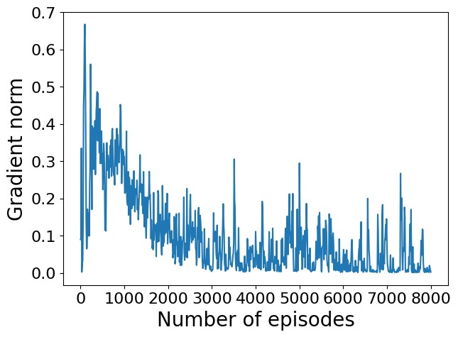
(a) Risk-neutral

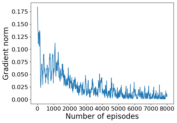
(b) Risk-averse $\beta=-0.1$

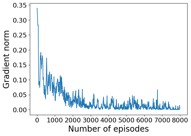
(c) Risk-averse $\beta=-0.2$

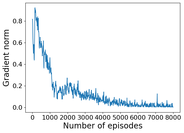
(d) Risk-averse $\beta=-0.5$

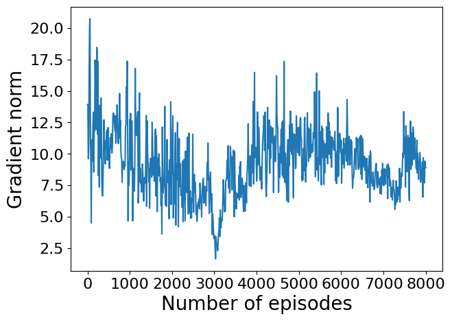
(e) Risk-averse $\beta=-10.0$

Figure 2: The gradient norm for risk-neutral and risk-averse with varying $\beta$ values.

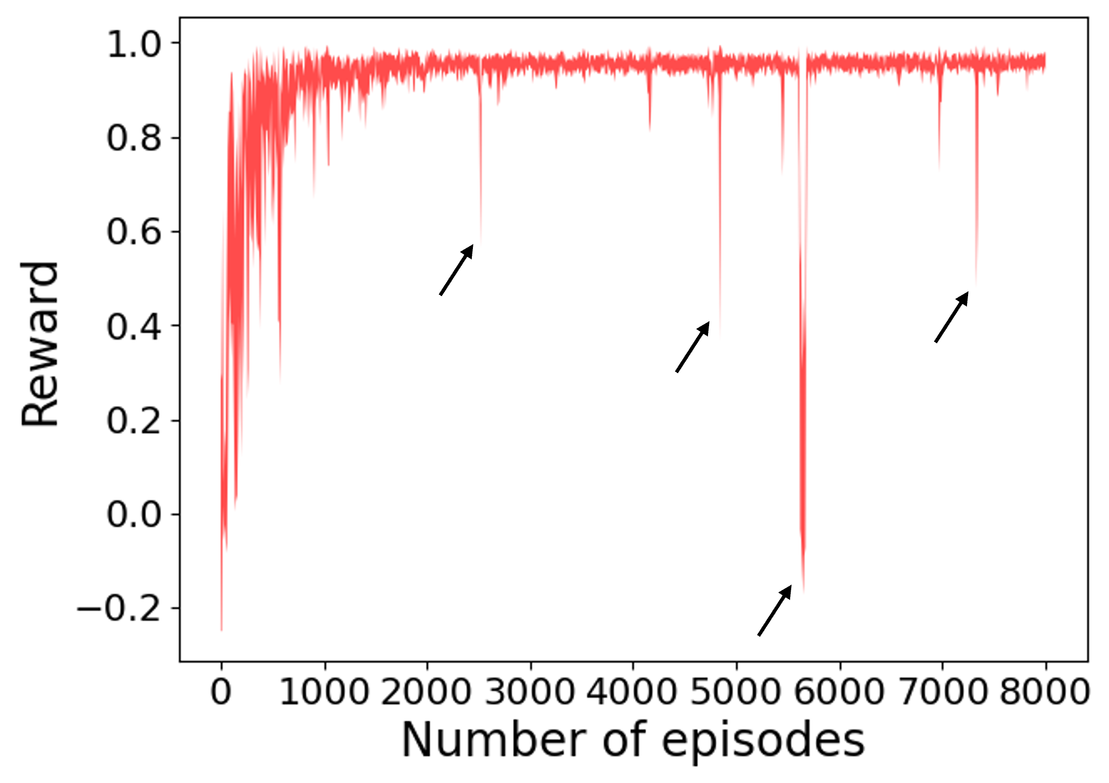
(a) Risk-neutral

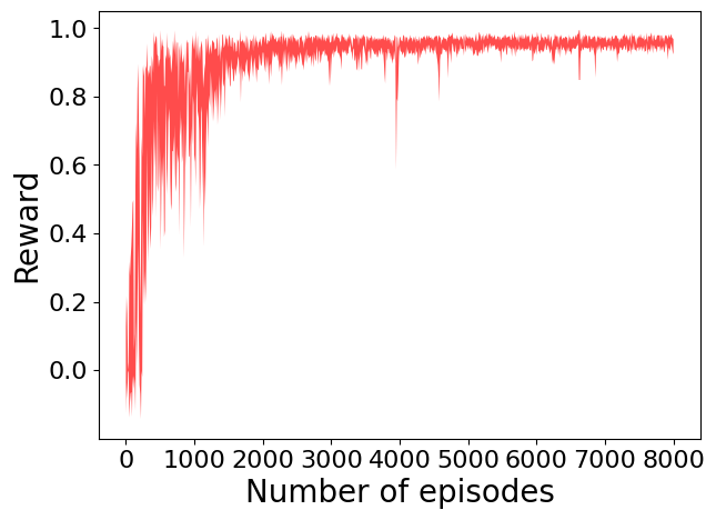
(b) Risk-averse $\beta=-0.1$

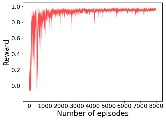
(c) Risk-averse $\beta=-0.2$

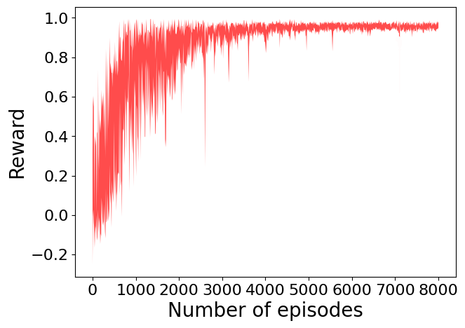
(d) Risk-averse $\beta=-0.5$

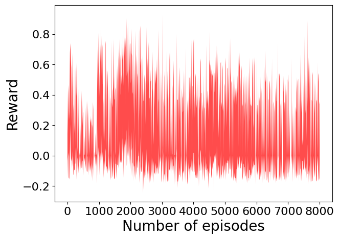
(e) Risk-averse $\beta=-10.0$

Figure 3: Learning curves of the reward for risk-neutral and risk-averse with varying $\beta$ values. Arrows in (a) depict extreme values.

In Figure 3, we illustrate the learning curves for the reward in the risk-neutral case and for different values of $\beta$ in the risk-averse cases. Although the acceleration effects for the risk-averse cases are not significant compared to the risk-neutral case, the risk-averse cases exhibit less variability and less significant extreme values, indicating that it requires fewer episodes to converge and stabilize. In contrast, the risk-neutral case displays more variability and more significant extreme values, as highlighted by arrows in Figure 3(a). As shown in Figure 3, the risk-averse case with $\beta=-0.1$ stabilizes after approximately 4000 episodes, the risk-averse cases with $\beta=-0.2,-0.5$ stabilize after around 3000 episodes, whereas this occurs after around 7300 episodes for the risk-neutral case. The number of episodes for convergence for risk-averse cases is approximately half of the number of episodes for convergence for the risk-neutral case. This observation verifies that risk-averse algorithms can achieve reduced iteration complexity, which also aligns well with Figure 2, illustrating that the risk-averse algorithm converges faster to a FOSP.

6 Conclusions

In this work, we start by analyzing the iteration complexity of the risk-sensitive REINFORCE algorithm, achieving an iteration complexity of ${\mathcal{O}}(\epsilon^{-2})$ aimed at attaining a First-Order Stationary Point (FOSP). This analysis extends an expected smoothness assumption from previous work and marks the first extension of iteration complexity analysis for the risk-sensitive REINFORCE algorithm. Next, we compare the iteration complexity of the risk-sensitive REINFORCE with its risk-neutral counterpart, which serves as a baseline. Our findings indicate that the risk-sensitive algorithm can achieve convergence with fewer iterations. We identify conditions under which the risk-sensitive algorithm may exhibit better iteration complexity. This finding is significant as it suggests that while considering risk during the decision-making process, we can simultaneously reduce the number of iterations required for learning. To validate our theoretical findings, we conduct simulation navigation experiments on Minigrid environment with varying risk-sensitive parameters. The results consistently support our theoretical findings, the number of episodes for convergence for all risk-averse cases can be approximately half of the episodes for convergence for the risk-neutral case.

Appendix

Appendix A Proof of Corollary 1

Proof.

Drawing inspiration from the proofs by Khaled & Richtárik (2020) and Yuan et al. (2022), we initiate our analysis by considering Assumption  1, which concerns Lipschitz smoothness. For the risk-sensitive objective $J_{\beta}$ with a Lipschitz smoothness constant $L_{\beta}$, we have that:

$$J_{\beta}(\theta_{t+1}) \geq J_{\beta}(\theta_{t})+\left<\nabla J_{\beta}(\theta_{t}),\theta_{t+1}-\theta_{t}\right>-\frac{L_{\beta}}{2}\left\|\theta_{t+1}-\theta_{t}\right\|^{2}$$ (34)

$$= J_{\beta}(\theta_{t})+\eta\left<\nabla J_{\beta}(\theta_{t}),\widehat{\nabla}J_{\beta}(\theta_{t})\right>-\frac{L_{\beta}\eta^{2}}{2}\left\|\widehat{\nabla}J_{\beta}(\theta_{t})\right\|^{2}.$$

Take expectations on both sides conditioned on $\theta_{t}$ and use Assumption 2, we get:

$$\mathbb{E}_{t}\left[J_{\beta}(\theta_{t+1})\right] \geq J_{\beta}(\theta_{t})+\eta\left<\nabla J_{\beta}(\theta_{t}),\nabla J_{\beta}(\theta_{t})\right>-\frac{L_{\beta}\eta^{2}}{2}\mathbb{E}_{t}\left[\left\|\widehat{\nabla}J_{\beta}(\theta_{t})\right\|^{2}\right]$$

$$\geq J_{\beta}(\theta_{t})+\eta\left\|\nabla J_{\beta}(\theta_{t})\right\|^{2}-\frac{L_{\beta}\eta^{2}}{2}\left(2A(J_{\beta}^{*}-J_{\beta}(\theta_{t}))+B\left\|\nabla J_{\beta}(\theta_{t})\right\|^{2}+C\right)$$

$$= J_{\beta}(\theta_{t})+\eta\left(1-\frac{L_{\beta}B\eta}{2}\right)\left\|\nabla J_{\beta}(\theta_{t})\right\|^{2}-L_{\beta}\eta^{2}A(J_{\beta}^{*}-J_{\beta}(\theta_{t}))-\frac{L_{\beta}C\eta^{2}}{2}.$$

Then we subtract $J_{\beta}^{*}$ from both sides,

$$\mathbb{E}_{t}\left[J_{\beta}(\theta_{t+1})\right]-J_{\beta}^{*} \geq -(1+L_{\beta}\eta^{2}A)(J_{\beta}^{*}-J_{\beta}(\theta_{t}))+\eta\left(1-\frac{L_{\beta}B\eta}{2}\right)\left\|\nabla J_{\beta}(\theta_{t})\right\|^{2}-\frac{L_{\beta}C\eta^{2}}{2}.$$ (36)

Take the expectation on both sides and rearrange the equation, we obtain:

$$\mathbb{E}\left[J_{\beta}^{*}-J_{\beta}(\theta_{t+1})\right]+\eta\left(1-\frac{L_{\beta}B\eta}{2}\right)\mathbb{E}\left[\left\|\nabla J_{\beta}(\theta_{t})\right\|^{2}\right]\leq(1+L_{\beta}\eta^{2}A)\mathbb{E}\left[J_{\beta}^{*}-J_{\beta}(\theta_{t})\right]+\frac{L_{\beta}C\eta^{2}}{2}.$$ (37)

Define $\delta_{t}\stackrel{{\scriptstyle\text{def}}}{{=}}\mathbb{E}\left[J_{\beta}^{*}-J_{\beta}(\theta_{t})\right]$ and $r_{t}\stackrel{{\scriptstyle\text{def}}}{{=}}\mathbb{E}\left[\left\|\nabla J_{\beta}(\theta_{t})\right\|^{2}\right]$, we can rewrite the above inequality as

$$\eta\left(1-\frac{L_{\beta}B\eta}{2}\right)r_{t} \leq (1+L_{\beta}\eta^{2}A)\delta_{t}-\delta_{t+1}+\frac{L_{\beta}C\eta^{2}}{2}.$$ (38)

Now, we introduce a sequence of weights, denoted as $w_{-1},w_{0},w_{1},\cdots,w_{T-1}$, based on a method used by (Stich, 2019; Khaled & Richtárik, 2020; Yuan et al., 2022). We initialize $w_{-1}$ with a positive value. We define $w_{t}$ as $w_{t}=\vcentcolon\frac{w_{t-1}}{1+L_{\beta}\eta^{2}A}$ for all $t\geq 0$. It’s important to note that when $A=0$, all $w_{t}$ are equal, i.e., $w_{t}=w_{t-1}=\cdots=w_{-1}$. By multiplying Equation 38 by $w_{t}/\eta$, we can derive:

$$\left(1-\frac{L_{\beta}B\eta}{2}\right)w_{t}r_{t} \leq \frac{w_{t}(1+L_{\beta}\eta^{2}A)}{\eta}\delta_{t}-\frac{w_{t}}{\eta}\delta_{t+1}+\frac{L_{\beta}C\eta}{2}w_{t}$$ (39)

$$= \frac{w_{t-1}}{\eta}\delta_{t}-\frac{w_{t}}{\eta}\delta_{t+1}+\frac{L_{\beta}C\eta}{2}w_{t}.$$

When we sum up both sides for $t=0,1,\cdots,T-1$, we get:

$$\left(1-\frac{L_{\beta}B\eta}{2}\right)\sum_{t=0}^{T-1}w_{t}r_{t} \leq \frac{w_{-1}}{\eta}\delta_{0}-\frac{w_{T-1}}{\eta}\delta_{T}+\frac{L_{\beta}C\eta}{2}\sum_{t=0}^{T-1}w_{t}$$ (40)

$$\leq \frac{w_{-1}}{\eta}\delta_{0}+\frac{L_{\beta}C\eta}{2}\sum_{t=0}^{T-1}w_{t}.$$

We can define $W_{T}$ as $W_{T}=\vcentcolon\sum_{t=0}^{T-1}w_{t}$. By dividing both sides of the equation by $W_{T}$, we obtain:

$$\left(1-\frac{L_{\beta}B\eta}{2}\right)\min_{0\leq t\leq T-1}r_{t}\leq\frac{1}{W_{T}}\cdot\left(1-\frac{L_{\beta}B\eta}{2}\right)\sum_{t=0}^{T-1}w_{t}r_{t}\leq\frac{w_{-1}}{W_{T}}\frac{\delta_{0}}{\eta}+\frac{L_{\beta}C\eta}{2}.$$ (41)

Note that,

$$W_{T}=\sum_{t=0}^{T-1}w_{t}\geq\sum_{t=0}^{T-1}\min_{0\leq i\leq T-1}w_{i}=Tw_{T-1}=\frac{Tw_{-1}}{(1+L_{\beta}\eta^{2}A)^{T}}.$$ (42)

Use this in Equation 41,

$$\left(1-\frac{L_{\beta}B\eta}{2}\right)\min_{0\leq t\leq T-1}r_{t} \leq \frac{(1+L\eta^{2}A)^{T}}{\eta T}\delta_{0}+\frac{LC\eta}{2}.$$ (43)

By substituting $r_{t}$ in Equation 43 with $\mathbb{E}\left[\left\|\nabla J_{\beta}(\theta_{t})\right\|^{2}\right]$, we obtain:

$$\left(1-\frac{L_{\beta}B\eta}{2}\right)\min_{0\leq t\leq T-1}\mathbb{E}\left[\left\|\nabla J_{\beta}(\theta_{t})\right\|^{2}\right] \leq \frac{(1+L_{\beta}\eta^{2}A)^{T}}{\eta T}\delta_{0}+\frac{L_{\beta}C\eta}{2},$$

$$\min_{0\leq t\leq T-1}\mathbb{E}\left[\left\|\nabla J_{\beta}(\theta_{t})\right\|^{2}\right] \leq \frac{2\delta_{0}(1+L_{\beta}\eta^{2}A)^{T}}{\eta T(2-L_{\beta}B\eta)}+\frac{L_{\beta}C\eta}{2-L_{\beta}B\eta}.$$ (44)

The choice of our step size ensures that for both cases, whether $B>0$ or $B=0$, we have $1-\frac{L_{\beta}B\eta}{2}>0$.

∎

Appendix B Proof of Theorem 1

Lemma 1.

Subject to Assumption 4, for any non-negative integer $t$, and for any state-action pair $(s_{t},a_{t})\in{\mathcal{S}}\times{\mathcal{A}}$ at time $t$ within a trajectory $\tau$ sampled under the parameterized policy $\pi_{\theta}$, we have the following:

$$\mathbb{E}_{\tau\sim p(\cdot\mid\theta)}\left[\left\|\nabla_{\theta}\log\pi_{\theta}(a_{t}\mid s_{t})\right\|^{2}\right] \leq F_{1}^{2},$$ (45)

$$\mathbb{E}_{\tau\sim p(\cdot\mid\theta)}\left[\left\|\nabla^{2}_{\theta}\log\pi_{\theta}(a_{t}\mid s_{t})\right\|\right] \leq F_{2}.$$ (46)

Proof.

For $t>0$ and $(s_{t},a_{t})\in{\mathcal{S}}\times{\mathcal{A}}$, we have

$$\mathbb{E}_{\tau}\left[\left\|\nabla_{\theta}\log\pi_{\theta}(a_{t}\mid s_{t})\right\|^{2}\right] =\mathbb{E}_{s_{t}}\left[\mathbb{E}_{a_{t}\sim\pi_{\theta}(\cdot\mid s_{t})}\left[\left\|\nabla_{\theta}\log\pi_{\theta}(a_{t}\mid s_{t})\right\|^{2}|s_{t}\right]\right]\overset{\ref{eq:G2}}{\leq}F_{1}^{2},$$ (47)

where the first equality is obtained by the Markov property. Similarly, we have

$$\mathbb{E}_{\tau}\left[\left\|\nabla_{\theta}^{2}\log\pi_{\theta}(a_{t}\mid s_{t})\right\|\right]=\mathbb{E}_{s_{t}}\left[\mathbb{E}_{a_{t}\sim\pi_{\theta}(\cdot\mid s_{t})}\left[\left\|\nabla_{\theta}^{2}\log\pi_{\theta}(a_{t}\mid s_{t})\right\||s_{t}\right]\right]\overset{\ref{eq:F}}{\leq}F_{2}.$$ (48)

∎

Then Lemma 1 is then used for the derivation of $L$ and $L_{\beta}$.

Assumption 1 is equivalent to $\left\|\nabla^{2}J(\theta)\right\|\leq L$ for the risk-neutral REINFORCE and $\left\|\nabla^{2}J_{\beta}(\theta)\right\|\leq L_{\beta}$ for the risk-sensitive REINFORCE. We first take the second order derivative of the risk-neutral objective w.r.t. $\theta$, in order to derive the $L$-Lipschitz smooth constant.

$$\nabla^{2}J(\theta) \overset{\ref{eq:pg}}{=} \nabla_{\theta}\mathbb{E}_{\tau}\left[\sum_{t=0}^{\infty}\nabla_{\theta}\log\pi_{\theta}(a_{t}\mid s_{t})R(t)\right]$$ (49)

$$= \nabla_{\theta}\Bigg{[}\int p(\tau\mid\theta)\sum_{t=0}^{\infty}\nabla_{\theta}\log\pi_{\theta}(a_{t}\mid s_{t})R(t)d\tau\Bigg{]}$$

$$= \int\nabla_{\theta}p(\tau\mid\theta)\left(\sum_{t=0}^{\infty}\nabla_{\theta}\log\pi_{\theta}(a_{t}\mid s_{t})R(t)\right)^{\top}d\tau+\int p(\tau\mid\theta)\sum_{t=0}^{\infty}\nabla_{\theta}^{2}\log\pi_{\theta}(a_{t}\mid s_{t})R(t)d\tau$$

$$= \int p(\tau\mid\theta)\nabla_{\theta}\log p(\tau\mid\theta)\left(\sum_{t=0}^{\infty}\nabla_{\theta}\log\pi_{\theta}(a_{t}\mid s_{t})R(t)\right)^{\top}d\tau+\int p(\tau\mid\theta)\sum_{t=0}^{\infty}\nabla_{\theta}^{2}\log\pi_{\theta}(a_{t}\mid s_{t})R(t)d\tau$$

$$= \mathbb{E}_{\tau}\left[\nabla_{\theta}\log p(\tau\mid\theta)\left(\sum_{t=0}^{\infty}\nabla_{\theta}\log\pi_{\theta}(a_{t}\mid s_{t})R(t)\right)^{\top}\right]+\mathbb{E}_{\tau}\left[\sum_{t=0}^{\infty}\nabla_{\theta}^{2}\log\pi_{\theta}(a_{t}\mid s_{t})R(t)\right]$$

$$\overset{\ref{eq:p}}{=} \underbrace{\mathbb{E}_{\tau}\left[\sum_{k=0}^{\infty}\nabla_{\theta}\log\pi_{\theta}(a_{k}\mid\theta_{k})\left(\sum_{t=0}^{\infty}\nabla_{\theta}\log\pi_{\theta}(a_{t}\mid s_{t})R(t)\right)^{\top}\right]}_{\leavevmode\hbox to7.49pt{\vbox to7.49pt{\text{[drawing]}}}}+\underbrace{\mathbb{E}_{\tau}\left[\sum_{t=0}^{\infty}\nabla_{\theta}^{2}\log\pi_{\theta}(a_{t}\mid s_{t})R(t)\right]}_{\leavevmode\hbox to7.49pt{\vbox to7.49pt{\text{[drawing]}}}}.$$

We individually bound the aforementioned two terms for the risk-neutral REINFORCE.

For the term ,

$$\left\|\leavevmode\hbox to9.93pt{\vbox to9.93pt{\text{[drawing]}}}\right\| = \left\|\mathbb{E}_{\tau}\left[\sum_{k=0}^{\infty}\nabla_{\theta}\log\pi_{\theta}(a_{k}\mid\theta_{k})\left(\sum_{t=0}^{\infty}\nabla_{\theta}\log\pi_{\theta}(a_{t}\mid s_{t})R(t)\right)^{\top}\right]\right\|$$ (50)

$$= \left\|\mathbb{E}_{\tau}\left[\sum_{k=0}^{\infty}\nabla_{\theta}\log\pi_{\theta}(a_{k}\mid\theta_{k})\left(\sum_{t=0}^{\infty}\nabla_{\theta}\log\pi_{\theta}(a_{t}\mid s_{t})\sum_{t^{\prime}=t}^{\infty}\gamma^{t^{\prime}}r(s_{t^{\prime}},a_{t^{\prime}})\right)^{\top}\right]\right\|$$

$$= \left\|\mathbb{E}_{\tau}\left[\sum_{t=0}^{\infty}\gamma^{t}r(s_{t},a_{t})\left(\sum_{t^{\prime}=0}^{t}\nabla_{\theta}\log\pi_{\theta}(a_{t^{\prime}}\mid\theta_{t^{\prime}})\right)\left(\sum_{k=0}^{t}\nabla_{\theta}\log\pi_{\theta}(a_{k}\mid\theta_{k})\right)^{\top}\right]\right\|$$

$$\leq \mathbb{E}_{\tau}\left[\sum_{t=0}^{\infty}\gamma^{t}\left|r(s_{t},a_{t})\right|\left\|\sum_{k=0}^{t}\nabla_{\theta}\log\pi_{\theta}(a_{k}\mid\theta_{k})\right\|^{2}\right]$$

$$\leq r_{max}\sum_{t=0}^{\infty}\gamma^{t}\sum_{k=0}^{t}\mathbb{E}_{\tau}\left[\left\|\nabla_{\theta}\log\pi_{\theta}(a_{k}\mid\theta_{k})\right\|^{2}\right]$$

$$\overset{\ref{eq:E_tau_F1}}{\leq} r_{max}F_{1}^{2}\sum_{t=0}^{\infty}\gamma^{t}(t+1)$$

$$= \frac{r_{max}F_{1}^{2}}{(1-\gamma)^{2}},$$

where the third line is due to the fact that the future actions do not depend on the past rewards.

For the term ,

$$\left\|\leavevmode\hbox to9.93pt{\vbox to9.93pt{\text{[drawing]}}}\right\| = \left\|\mathbb{E}_{\tau}\left[\sum_{t=0}^{\infty}\nabla_{\theta}^{2}\log\pi_{\theta}(a_{t}\mid s_{t})R(t)\right]\right\|$$ (51)

$$= \left\|\mathbb{E}_{\tau}\left[\sum_{t=0}^{\infty}\nabla_{\theta}^{2}\log\pi_{\theta}(a_{t}\mid s_{t})\sum_{t^{\prime}=t}^{\infty}\gamma^{t^{\prime}}r(s_{t^{\prime}},a_{t^{\prime}})\right]\right\|$$

$$= \left\|\mathbb{E}_{\tau}\left[\sum_{t=0}^{\infty}\gamma^{t}r(s_{t},a_{t})\left(\sum_{k=0}^{t}\nabla_{\theta}^{2}\log\pi_{\theta}(a_{k}\mid s_{k})\right)\right]\right\|$$

$$\leq \mathbb{E}_{\tau}\left[\sum_{t=0}^{\infty}\gamma^{t}\left|r(s_{t},a_{t})\right|\left(\sum_{k=0}^{t}\left\|\nabla_{\theta}^{2}\log\pi_{\theta}(a_{k}\mid s_{k})\right\|\right)\right]$$

$$\leq r_{\max}\sum_{t=0}^{\infty}\gamma^{t}\left(\sum_{k=0}^{t}\mathbb{E}_{\tau}\left[\left\|\nabla_{\theta}^{2}\log\pi_{\theta}(a_{k}\mid s_{k})\right\|\right]\right)$$

$$\overset{\ref{eq:E_tau_F2}}{\leq} r_{\max}F_{2}\sum_{t=0}^{\infty}\gamma^{t}(t+1)$$

$$= \frac{r_{\max}F_{2}}{(1-\gamma)^{2}},$$

where the third line is also due to the fact that the future actions do not depend on the past rewards.

Finally,

$$\left\|\nabla^{2}J(\theta)\right\|\leq\frac{r_{\max}}{(1-\gamma)^{2}}(F_{1}^{2}+F_{2}),$$ (52)

so $L=\frac{r_{\max}}{(1-\gamma)^{2}}(F_{1}^{2}+F_{2})$.

Then we take the second order derivative of the risk-sensitive objective w.r.t. $\theta$, in order to derive the $L_{\beta}$-Lipschitz smoothness constant.

$$\nabla^{2}J_{\beta}(\theta) \overset{\ref{eq:risk-pg}}{=} \nabla_{\theta}\mathbb{E}_{\tau}\left[\sum_{t=0}^{\infty}\nabla_{\theta}\log\pi_{\theta}(a_{t}\mid s_{t})\cdot\beta e^{\beta R(t)}\right]$$ (53)

$$= \nabla_{\theta}\Bigg{[}\int p(\tau\mid\theta)\sum_{t=0}^{\infty}\nabla_{\theta}\log\pi_{\theta}(a_{t}\mid s_{t})\cdot\beta e^{\beta R(t)}d\tau\Bigg{]}$$

$$= \int\nabla_{\theta}p(\tau\mid\theta)\left(\sum_{t=0}^{\infty}\nabla_{\theta}\log\pi_{\theta}(a_{t}\mid s_{t})\cdot\beta e^{\beta R(t)}\right)^{\top}d\tau+\int p(\tau\mid\theta)\sum_{t=0}^{\infty}\nabla_{\theta}^{2}\log\pi_{\theta}(a_{t}\mid s_{t})\cdot\beta e^{\beta R(t)}d\tau$$

$$= \int p(\tau\mid\theta)\nabla_{\theta}\log p(\tau\mid\theta)\left(\sum_{t=0}^{\infty}\nabla_{\theta}\log\pi_{\theta}(a_{t}\mid s_{t})\cdot\beta e^{\beta R(t)}\right)^{\top}d\tau$$

$$+\int p(\tau\mid\theta)\sum_{t=0}^{\infty}\nabla_{\theta}^{2}\log\pi_{\theta}(a_{t}\mid s_{t})\cdot\beta e^{\beta R(t)}d\tau$$

$$= \mathbb{E}_{\tau}\left[\nabla_{\theta}\log p(\tau\mid\theta)\left(\sum_{t=0}^{\infty}\nabla_{\theta}\log\pi_{\theta}(a_{t}\mid s_{t})\cdot\beta e^{\beta R(t)}\right)^{\top}\right]+\mathbb{E}_{\tau}\left[\sum_{t=0}^{\infty}\nabla_{\theta}^{2}\log\pi_{\theta}(a_{t}\mid s_{t})\cdot\beta e^{\beta R(t)}\right]$$

$$\overset{\ref{eq:p}}{=} \underbrace{\mathbb{E}_{\tau}\left[\sum_{k=0}^{\infty}\nabla_{\theta}\log\pi_{\theta}(a_{k}\mid\theta_{k})\left(\sum_{t=0}^{\infty}\nabla_{\theta}\log\pi_{\theta}(a_{t}\mid s_{t})\cdot\beta e^{\beta R(t)}\right)^{\top}\right]}_{\leavevmode\hbox to7.49pt{\vbox to7.49pt{\text{[drawing]}}}}$$

$$+\underbrace{\mathbb{E}_{\tau}\left[\sum_{t=0}^{\infty}\nabla_{\theta}^{2}\log\pi_{\theta}(a_{t}\mid s_{t})\cdot\beta e^{\beta R(t)}\right]}_{\leavevmode\hbox to7.49pt{\vbox to7.49pt{\text{[drawing]}}}}.$$

We also bound the above two terms separately for the risk-sensitive REINFORCE algorithm.

For the term ,

$$\left\|\leavevmode\hbox to9.93pt{\vbox to9.93pt{\text{[drawing]}}}\right\| = \left\|\mathbb{E}_{\tau}\left[\sum_{k=0}^{\infty}\nabla_{\theta}\log\pi_{\theta}(a_{k}\mid\theta_{k})\left(\sum_{t=0}^{\infty}\nabla_{\theta}\log\pi_{\theta}(a_{t}\mid s_{t})\cdot\beta e^{\beta R(t)}\right)^{\top}\right]\right\|$$ (54)

$$= \left\|\mathbb{E}_{\tau}\left[\sum_{k=0}^{\infty}\nabla_{\theta}\log\pi_{\theta}(a_{k}\mid\theta_{k})\left(\sum_{t=0}^{\infty}\nabla_{\theta}\log\pi_{\theta}(a_{t}\mid s_{t})\cdot\beta e^{\beta\sum_{t^{\prime}=t}^{\infty}\gamma^{t^{\prime}}r(s_{t^{\prime}},a_{t^{\prime}})}\right)^{\top}\right]\right\|$$

$$= \left\|\mathbb{E}_{\tau}\left[\beta e^{\beta\sum_{t=0}^{\infty}\gamma^{t}r(s_{t},a_{t})}\left(\sum_{t^{\prime}=0}^{t}\nabla_{\theta}\log\pi_{\theta}(a_{t^{\prime}}\mid\theta_{t^{\prime}})\right)\left(\sum_{k=0}^{t}\nabla_{\theta}\log\pi_{\theta}(a_{k}\mid\theta_{k})\right)^{\top}\right]\right\|$$

$$\leq \mathbb{E}_{\tau}\left[|\beta|e^{|\beta|\sum_{t=0}^{\infty}\gamma^{t}\left|r(s_{t},a_{t})\right|}\left\|\sum_{k=0}^{t}\nabla_{\theta}\log\pi_{\theta}(a_{k}\mid\theta_{k})\right\|^{2}\right]$$

$$\overset{\ref{eq: ratio}}{=} \mathbb{E}_{\tau}\left[\alpha\sum_{t=0}^{\infty}\gamma^{t}|r(s_{t},a_{t})|\left\|\sum_{k=0}^{t}\nabla_{\theta}\log\pi_{\theta}(a_{k}\mid\theta_{k})\right\|^{2}\right]$$

$$\leq \alpha\cdot r_{max}\sum_{t=0}^{\infty}\gamma^{t}\mathbb{E}_{\tau}\left[\left\|\sum_{k=0}^{t}\nabla_{\theta}\log\pi_{\theta}(a_{k}\mid\theta_{k})\right\|^{2}\right]$$

$$= \alpha\cdot r_{max}\sum_{t=0}^{\infty}\gamma^{t}\sum_{k=0}^{t}\mathbb{E}_{\tau}\left[\left\|\nabla_{\theta}\log\pi_{\theta}(a_{k}\mid\ \theta_{k})\right\|^{2}\right]$$

$$\leq \alpha\cdot r_{max}F_{1}^{2}\sum_{t=0}^{\infty}\gamma^{t}(t+1)$$

$$= \alpha\cdot\frac{r_{max}F_{1}^{2}}{(1-\gamma)^{2}},$$

where in the third line, we use the fact that the future actions do not depend on the past rewards. In the fifth line, we use Assumption 3.

For the term ,

$$\left\|\leavevmode\hbox to9.93pt{\vbox to9.93pt{\text{[drawing]}}}\right\| = \left\|\mathbb{E}_{\tau}\left[\sum_{t=0}^{\infty}\nabla_{\theta}^{2}\log\pi_{\theta}(a_{t}\mid s_{t})\cdot\beta e^{\beta R(t)}\right]\right\|$$ (55)

$$= \left\|\mathbb{E}_{\tau}\left[\sum_{t=0}^{\infty}\nabla_{\theta}^{2}\log\pi_{\theta}(a_{t}\mid s_{t})\cdot\beta e^{\beta\sum_{t^{\prime}=t}^{\infty}\gamma^{t^{\prime}}r(s_{t^{\prime}},a_{t^{\prime}})}\right]\right\|$$

$$= \left\|\mathbb{E}_{\tau}\left[\beta e^{\beta\sum_{t=0}^{\infty}\gamma^{t}r(s_{t},a_{t})}\left(\sum_{k=0}^{t}\nabla_{\theta}^{2}\log\pi_{\theta}(a_{k}\mid s_{k})\right)\right]\right\|$$

$$\leq \mathbb{E}_{\tau}\left[|\beta|e^{|\beta|\sum_{t=0}^{\infty}\gamma^{t}|r(s_{t},a_{t})|}\left(\sum_{k=0}^{t}\left\|\nabla_{\theta}^{2}\log\pi_{\theta}(a_{k}\mid s_{k})\right\|\right)\right]$$

$$\overset{\ref{eq: ratio}}{=} \mathbb{E}_{\tau}\left[\alpha\cdot\sum_{t=0}^{\infty}\gamma^{t}|r(s_{t},a_{t})|\left(\sum_{k=0}^{t}\left\|\nabla_{\theta}^{2}\log\pi_{\theta}(a_{k}\mid s_{k})\right\|\right)\right]$$

$$\leq \alpha\cdot r_{\max}\sum_{t=0}^{\infty}\gamma^{t}\left(\sum_{k=0}^{t}\mathbb{E}_{\tau}\left[\left\|\nabla_{\theta}^{2}\log\pi_{\theta}(a_{k}\mid s_{k})\right\|\right]\right)$$

$$\overset{\ref{eq:E_tau_F2}}{\leq} \alpha\cdot r_{\max}F_{2}\sum_{t=0}^{\infty}\gamma^{t}(t+1)$$

$$= \alpha\cdot\frac{r_{\max}F_{2}}{(1-\gamma)^{2}}$$

Finally,

$$\left\|\nabla^{2}J_{\beta}(\theta)\right\|\leq\alpha\cdot\frac{r_{\max}}{(1-\gamma)^{2}}(F_{1}^{2}+F_{2}),$$ (56)

so $L_{\beta}=\alpha\cdot\frac{r_{\max}}{(1-\gamma)^{2}}(F_{1}^{2}+F_{2})$, where $0<\alpha<1$.

References

- AlMahamid & Grolinger (2021) Fadi AlMahamid and Katarina Grolinger. Reinforcement learning algorithms: An overview and classification. In 2021 IEEE Canadian Conference on Electrical and Computer Engineering (CCECE), pp. 1–7. IEEE, 2021.
- Baxter & Bartlett (2001) Jonathan Baxter and Peter L Bartlett. Infinite-horizon policy-gradient estimation. journal of artificial intelligence research, 15:319–350, 2001.
- Berkenkamp et al. (2017) Felix Berkenkamp, Matteo Turchetta, Angela Schoellig, and Andreas Krause. Safe model-based reinforcement learning with stability guarantees. Advances in neural information processing systems, 30, 2017.
- Casper et al. (2023) Stephen Casper, Xander Davies, Claudia Shi, Thomas Krendl Gilbert, Jérémy Scheurer, Javier Rando, Rachel Freedman, Tomasz Korbak, David Lindner, Pedro Freire, et al. Open problems and fundamental limitations of reinforcement learning from human feedback. arXiv preprint arXiv:2307.15217, 2023.
- Charpentier et al. (2021) Arthur Charpentier, Romuald Elie, and Carl Remlinger. Reinforcement learning in economics and finance. Computational Economics, pp. 1–38, 2021.
- Chevalier-Boisvert et al. (2023) Maxime Chevalier-Boisvert, Bolun Dai, Mark Towers, Rodrigo de Lazcano, Lucas Willems, Salem Lahlou, Suman Pal, Pablo Samuel Castro, and Jordan Terry. Minigrid & miniworld: Modular & customizable reinforcement learning environments for goal-oriented tasks. CoRR, abs/2306.13831, 2023.
- Dann & Brunskill (2015) Christoph Dann and Emma Brunskill. Sample complexity of episodic fixed-horizon reinforcement learning. Advances in Neural Information Processing Systems, 28, 2015.
- Eriksson & Dimitrakakis (2019) Hannes Eriksson and Christos Dimitrakakis. Epistemic risk-sensitive reinforcement learning. arXiv preprint arXiv:1906.06273, 2019.
- Fei et al. (2020) Yingjie Fei, Zhuoran Yang, Yudong Chen, Zhaoran Wang, and Qiaomin Xie. Risk-sensitive reinforcement learning: Near-optimal risk-sample tradeoff in regret. Advances in Neural Information Processing Systems, 33:22384–22395, 2020.
- Filos (2019) Angelos Filos. Reinforcement learning for portfolio management. arXiv preprint arXiv:1909.09571, 2019.
- Hau et al. (2023) Jia Lin Hau, Marek Petrik, and Mohammad Ghavamzadeh. Entropic risk optimization in discounted mdps. In International Conference on Artificial Intelligence and Statistics, pp. 47–76. PMLR, 2023.
- Jain et al. (2017) Prateek Jain, Purushottam Kar, et al. Non-convex optimization for machine learning. Foundations and Trends® in Machine Learning, 10(3-4):142–363, 2017.
- Kaelbling et al. (1996) Leslie Pack Kaelbling, Michael L Littman, and Andrew W Moore. Reinforcement learning: A survey. Journal of artificial intelligence research, 4:237–285, 1996.
- Kakade (2001) Sham M Kakade. A natural policy gradient. Advances in neural information processing systems, 14, 2001.
- Kakade (2003) Sham Machandranath Kakade. On the sample complexity of reinforcement learning. University of London, University College London (United Kingdom), 2003.
- Khaled & Richtárik (2020) Ahmed Khaled and Peter Richtárik. Better theory for sgd in the nonconvex world. arXiv preprint arXiv:2002.03329, 2020.
- Kingma & Ba (2014) Diederik P Kingma and Jimmy Ba. Adam: A method for stochastic optimization. arXiv preprint arXiv:1412.6980, 2014.
- Lattimore et al. (2013) Tor Lattimore, Marcus Hutter, and Peter Sunehag. The sample-complexity of general reinforcement learning. In International Conference on Machine Learning, pp. 28–36. PMLR, 2013.
- Lee et al. (2020) Jaeho Lee, Sejun Park, and Jinwoo Shin. Learning bounds for risk-sensitive learning. Advances in Neural Information Processing Systems, 33:13867–13879, 2020.
- Liu et al. (2023) Rui Liu, Guangyao Shi, and Pratap Tokekar. Data-driven distributionally robust optimal control with state-dependent noise. arXiv preprint arXiv:2303.02293, 2023.
- Majumdar et al. (2017) Anirudha Majumdar, Sumeet Singh, Ajay Mandlekar, and Marco Pavone. Risk-sensitive inverse reinforcement learning via coherent risk models. In Robotics: science and systems, volume 16, pp. 117, 2017.
- Mihatsch & Neuneier (2002) Oliver Mihatsch and Ralph Neuneier. Risk-sensitive reinforcement learning. Machine learning, 49:267–290, 2002.
- Mnih et al. (2013) Volodymyr Mnih, Koray Kavukcuoglu, David Silver, Alex Graves, Ioannis Antonoglou, Daan Wierstra, and Martin Riedmiller. Playing atari with deep reinforcement learning. arXiv preprint arXiv:1312.5602, 2013.
- Noorani & Baras (2021) Erfaun Noorani and John S Baras. Risk-sensitive reinforce: A monte carlo policy gradient algorithm for exponential performance criteria. In 2021 60th IEEE Conference on Decision and Control (CDC), pp. 1522–1527. IEEE, 2021.
- Noorani et al. (2022) Erfaun Noorani, Christos Mavridis, and John Baras. Risk-sensitive reinforcement learning with exponential criteria. arXiv preprint arXiv:2212.09010, 2022.
- Papini (2021) Matteo Papini. Safe policy optimization. 2021.
- Papini et al. (2018) Matteo Papini, Damiano Binaghi, Giuseppe Canonaco, Matteo Pirotta, and Marcello Restelli. Stochastic variance-reduced policy gradient. In International conference on machine learning, pp. 4026–4035. PMLR, 2018.
- Prashanth et al. (2022) LA Prashanth, Michael C Fu, et al. Risk-sensitive reinforcement learning via policy gradient search. Foundations and Trends® in Machine Learning, 15(5):537–693, 2022.
- Qiu et al. (2021) Wei Qiu, Xinrun Wang, Runsheng Yu, Rundong Wang, Xu He, Bo An, Svetlana Obraztsova, and Zinovi Rabinovich. Rmix: Learning risk-sensitive policies for cooperative reinforcement learning agents. Advances in Neural Information Processing Systems, 34:23049–23062, 2021.
- Shen et al. (2014) Yun Shen, Michael J Tobia, Tobias Sommer, and Klaus Obermayer. Risk-sensitive reinforcement learning. Neural computation, 26(7):1298–1328, 2014.
- Silver et al. (2016) David Silver, Aja Huang, Chris J Maddison, Arthur Guez, Laurent Sifre, George Van Den Driessche, Julian Schrittwieser, Ioannis Antonoglou, Veda Panneershelvam, Marc Lanctot, et al. Mastering the game of go with deep neural networks and tree search. nature, 529(7587):484–489, 2016.
- Stich (2019) Sebastian U Stich. Unified optimal analysis of the (stochastic) gradient method. arXiv preprint arXiv:1907.04232, 2019.
- Sutton & Barto (2018) Richard S Sutton and Andrew G Barto. Reinforcement learning: An introduction. MIT press, 2018.
- Sutton et al. (1999) Richard S Sutton, David McAllester, Satinder Singh, and Yishay Mansour. Policy gradient methods for reinforcement learning with function approximation. Advances in neural information processing systems, 12, 1999.
- Williams (1992) Ronald J Williams. Simple statistical gradient-following algorithms for connectionist reinforcement learning. Machine learning, 8:229–256, 1992.
- Xu et al. (2019) Pan Xu, Felicia Gao, and Quanquan Gu. Sample efficient policy gradient methods with recursive variance reduction. arXiv preprint arXiv:1909.08610, 2019.
- Xu et al. (2020) Pan Xu, Felicia Gao, and Quanquan Gu. An improved convergence analysis of stochastic variance-reduced policy gradient. In Uncertainty in Artificial Intelligence, pp. 541–551. PMLR, 2020.
- Yuan et al. (2022) Rui Yuan, Robert M Gower, and Alessandro Lazaric. A general sample complexity analysis of vanilla policy gradient. In International Conference on Artificial Intelligence and Statistics, pp. 3332–3380. PMLR, 2022.
- Zhang et al. (2021) Lixian Zhang, Ruixian Zhang, Tong Wu, Rui Weng, Minghao Han, and Ye Zhao. Safe reinforcement learning with stability guarantee for motion planning of autonomous vehicles. IEEE Transactions on Neural Networks and Learning Systems, 32(12):5435–5444, 2021.