Rollover Prevention for Mobile Robots with Control Barrier Functions: Differentiator-Based Adaptation and Projection-to-State Safety

Abstract

This paper develops rollover prevention guarantees for mobile robots using control barrier function (CBF) theory, and demonstrates these formal results experimentally. To this end, we consider a safety measure based on the zero moment point to provide conditions on the control input through the lens of CBFs. However, these conditions depend on time-varying and noisy parameters. To address this, we present a differentiator-based safety-critical controller that estimates these parameters and pairs Input-to-State Stable (ISS) differentiator dynamics with CBFs to achieve rigorous guarantees of safety. Additionally, to ensure safety in the presence of disturbance, we utilize a time-varying extension of Projection-to-State Safety (PSSf). The effectiveness of the proposed method is demonstrated through experiments on a tracked robot with a rollover potential on steep slopes.

I Introduction

Autonomous robotic systems are being increasingly deployed in real-world environments, marking a corresponding rise in the importance of developing safety-critical control methods. This is especially true of mobile robots operating in diverse environments [1]. One critical aspect of safety in mobile robotic systems is the prevention of rollover. As mobile robots often operate on uneven terrains and dynamic conditions, preventing rollover is a vital aspect of their design and operation [2]. Addressing concerns related to rollover in mobile robotics not only improves the overall safety of these systems but also significantly contributes to their reliability and effectiveness in real-world applications.

Several methods have been developed to measure the risk of rollover in mobile robots, including stability measures like force-angle stability, moment-height stability, and zero moment point (ZMP) [3]. Leveraging these characterizations, a variety of control techniques have been developed to prevent rollovers: nonlinear programming [4], chance-constrained optimal control [5], and invariance control [6]. These methods often rely on high-fidelity models or require numerous sensors, which may limit their practical applicability in real-world scenarios. The goal of this paper is to develop a new approach for rollover avoidance that is both rigorous, but also implementable.

Safety is often framed as forward set invariance; guaranteeing that system states stay within a predetermined set ensures that the system is safe. Control barrier functions (CBFs) [7] have emerged as a tool for synthesizing controllers guaranteeing that a given safe set is forward invariant. The CBF framework also leads to safety filters, which have been successfully applied in various domains [8]. These filters alter control inputs only when it is necessary for safety. However, accurate information on system dynamics is necessary for safety guarantees provided by a controller synthesized via CBFs. Thus, the presence of unmodeled dynamics in the system causes uncertainty in the CBF condition, potentially leading to safety constraint violation.

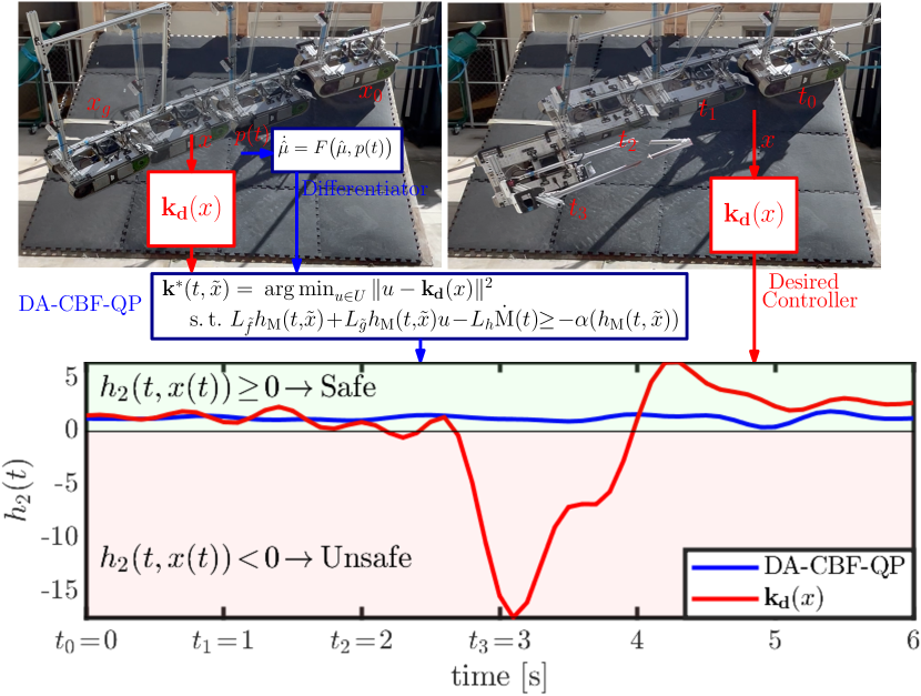
Figure 1: Experimental results for rollover prevention in a mobile robot. The proposed DA-CBF-QP-based safety filter maintains safety (left, video montage of robot motion). However, the robot under the desired controller leaves the safe set (Right). The value of CBF $h$ vs. time (Bottom).

To establish a framework to quantify the effect of uncertainty or disturbances on safety guarantees, the framework of Projection-to-State Safety (PSSf) [9] was introduced building upon the notion of Input-to-State Safety (ISSf) [10]. Yet in the setting of rollover avoidance, ZMP-based rollover constraints require information on the dynamically evolving environment; more specifically, the derivative of the gravity vector needs to be estimated for the CBF conditions. Safety-critical control in dynamic environments via CBFs was proposed in [11] by using constant worst-case bounds for the time-varying parameters, which may result in undesired conservativeness. CBFs coupled with estimators can address the moving obstacles avoidance problem [12]. However, the extension to address broader dynamic parameter-dependent safe control design problems has not yet been considered.

This paper presents a theoretic framework for the synthesis of safety filters that are robust to time-varying parameters, and applies this experimentally to achieve rollover prevention on a mobile robot (Fig. 1). Formally, we introduce the notion of differentiator-adaptive CBFs (DA-CBFs) that consider the time-derivatives of time-varying parameters that are necessary to enforce CBF conditions. When the dynamics of the differentiator is ISS with respect to noise, the result is a new time-varying CBF whose satisfaction ensures safety. Moreover, to address model uncertainty in the time derivative of a time-varying CBF, we define an extension of PSSf, time-varying PSSf (tPSSf). The main result gives conditions on DA-CBFs such that PSSf is guaranteed. Practically, these contributions enable the development of robust rollover prevention for mobile robots via the synthesis of CBFs from ZMP constraints. We validate the efficacy of the proposed approach through experiments conducted on a tracked robot encountering rollover issues triggered by slopes.

This paper is organized as follows. Section II provides a review of CBFs. Section III introduces DA-CBFs and tPSSf. Section IV presents the theory and practical implementation of rollover prevention.

II Preliminaries

Consider a nonlinear control affine system of the form:

$$\dot{x}=f(x)+g(x)u,$$ (1)

where ${x\!\in\!X\!\subset\!\mathbb{R}^{n}}$ is the state, ${f\!:\!X\!\to\!\mathbb{R}^{n}}$, ${g\!:\!X\!\to\!\mathbb{R}^{n\times m}}$ are locally Lipschitz continuous functions on $X$, and ${u\!\in\!U\!\subset\!\mathbb{R}^{m}}$ is the control input. A locally Lipschitz continuous controller ${\mathbf{k}\!:\!X\!\to\!U}$ yields a locally Lipschitz continuous closed-loop control system, ${f_{\rm cl}\!:\!X\!\to\!\mathbb{R}^{n}}$:

$$\dot{x}={f}(x)+{g}(x)\mathbf{k}(x)\triangleq f_{\rm cl}(x).$$ (2)

Hence, given any initial condition ${x_{0}\!\triangleq\!x(t_{0})\!\in\!X}$ there exists an interval $\mathcal{I}({x}_{0})\!\triangleq\!\left[t_{0},t_{\max}\right)$ such that

$${x}(t)=x_{0}+\int^{t}_{t_{0}}f_{\rm cl}(x(\tau))d\tau,~{}t>t_{0}$$ (3)

is the unique solution to (2) for ${t\!\in\!\mathcal{I}({x}_{0})}$; see [13]. Throughout this study we assume ${f_{\rm cl}}$ is forward complete, i.e., ${\mathcal{I}({x}_{0})\!=\![0,\infty)}$, and ${U}$ is a convex polytope.

In this paper, the notion of safety is defined by identifying a safe set within the state space. The system is considered safe as long as its states stay within this set. Let set ${\mathcal{C}\!\subset\!X}$ be the 0-superlevel set of a continuously differentiable function ${h\!:\!X\!\to\!\mathbb{R}}$:

$$\begin{split}\mathcal{C}\triangleq\left\{x\!\in\!X\!\subset\!\mathbb{R}^{n}:h(x)\geq 0\right\},\\ \partial\mathcal{C}\triangleq\left\{{x\!\in\!X\!\subset\!\mathbb{R}^{n}}:h(x)=0\right\}.\end{split}$$ (4)

This set is forward invariant if, for any initial condition ${x(0)\!\in\!\mathcal{C}}$, the solution (3) satisfies ${x(t)\!\in\!\mathcal{C},~{}\forall t\!\geq\!0}$. The closed-loop system (2) is said to be safe on the set $\mathcal{C}$ if $\mathcal{C}$ is forward invariant. We call $\mathcal{C}$ the safe set. CBFs [7] have been proposed to synthesize safety-critical controllers that can ensure forward invariance.

Definition 1 (Control Barrier Function [7]).

Let ${\mathcal{C}\!\subset\!X}$ be the 0-superlevel set of a continuously differentiable function ${h\!:\!X\!\to\!\mathbb{R}}$. The function $h$ is a control barrier function for system (1) on $\mathcal{C}$ if ${\frac{\partial h}{\partial x}\neq 0}$ for all ${x\!\in\!\partial\mathcal{C}}$ and there exists an extended class-$\mathcal{K}_{\infty}$ function $\alpha\!\in\!\mathcal{K}_{\infty,e}$ such that $\forall x\!\in\!\mathcal{C}$:

$$\sup_{u\in U}\big{[}{\dot{h}(x,u)}\big{]}\!=\!\sup_{u\in U}\big{[}L_{f}h(x)+L_{g}h(x)u\big{]}\!\geq\!-\alpha(h(x)),$$ (5)

where ${L_{f}h\!:\!X\!\to\!\mathbb{R}}$, ${L_{g}h\!:\!X\!\to\!\mathbb{R}^{m}}$ are Lie derivatives.

Note that, when ${U\!=\!\mathbb{R}^{m}}$, (5) is equivalent to:

$$\forall x\!\in\!X\!:\ L_{g}h(x)=0\implies L_{f}h(x)\geq-\alpha(h(x)),$$ (6)

which implies that if ${U\!=\!\mathbb{R}^{m}}$, satisfaction of condition (5) at states where ${L_{g}h(x)\!=\!0}$ is necessary and sufficient for the verification of a CBF. We note that for a bounded control input, i.e., ${u\!\in\!U\!\subset\!\mathbb{R}^{m}}$, (6) is a necessary (but not sufficient) condition for (5).

Given a CBF ${h}$ and a corresponding ${\alpha}$ for (1), the pointwise set of all control values that satisfy (5) is given by

$$K_{\text{CBF}}(x)\triangleq\big{\{}u\in U\big{|}\dot{h}(x,u)\geq-\alpha(h(x))\big{\}}.$$

We can establish formal safety guarantees based on Definition 1 with the help of the following theorem [7]:

Theorem 1.

If $h$ is a CBF for (1) on $\mathcal{C}$ with an ${\alpha\!\in\!\mathcal{K}_{\infty,e}}$, then any Lipschitz continuous controller ${\mathbf{k}\!:\!X\!\to\!U}$ satisfying

$$\dot{h}\left(x,\mathbf{k}(x)\right)\geq-\alpha(h(x)),~{}~{}\forall x\in\mathcal{C},$$ (7)

renders (2) safe with respect to $\mathcal{C}$.

Given a nominal (possibly unsafe) locally Lipschitz continuous desired controller $\mathbf{k_{d}}\!:\!X\!\to\!U$, and a CBF ${h}$ with a corresponding ${\alpha}$ for system (1), safety can be ensured by solving the CBF-Quadratic Program (CBF-QP) [7]:

$$\begin{array}[]{l}{\mathbf{k^{*}}(x)=\ }\displaystyle\operatorname*{arg\,min}_{{u}\in U}\ \ \ {\|u-\mathbf{k_{d}}(x)\|^{2}}\\[2.84526pt] ~{}~{}~{}~{}~{}~{}~{}~{}~{}~{}~{}~{}\textrm{s.t.}~{}~{}~{}~{}~{}~{}~{}~{}~{}\dot{h}(x,u)\geq-\alpha(h(x)),\end{array}$$

which enforces ${\mathbf{k^{*}}\!:\!X\!\to\!U}$ to take values in ${K_{\text{CBF}}(x)}$; thus, CBF-QP is also called a safety filter. Note that when ${\mathbf{k^{*}}(x)\!\in\!K_{\text{CBF}}(x)}$ for all ${x\!\in\!X}$, the set ${\mathcal{C}}$ is asymptotically stable for the forward complete closed-loop system ${f_{\rm cl}}$ in ${X}$. Thus, the safety filter ensures that the closed-loop system asymptotically approaches ${\mathcal{C}}$ even if the initial states do not satisfy the CBF condition in CBF-QP, i.e., ${x_{0}\notin\mathcal{C}}$ [7].

III Main Result

This section first defines tPSSf to consider model uncertainty in the time derivative of a time-varying CBF. Then, we introduce DA-CBFs.

In practice, control systems face uncertainties and disturbances that cannot be fully modeled. Thus, we consider a disturbed nonlinear control affine system:

$$\dot{x}=f(x)+g(x)u+d(t),$$ (8)

where ${d\!:\!\mathbb{R}^{+}_{0}\!\to\!\mathbb{R}^{n}}$ is the disturbance that can alter the safety property endowed by the CBF for system (1).

For the sake of generality, we consider a time-varying continuously differentiable function ${h\!:\!\mathbb{R}^{+}_{0}\!\times\!X\!\to\!\mathbb{R}}$, and its 0-superlevel set given by

$$\mathcal{C}(t)\triangleq\big{\{}x\!\in\!X:h(t,x)\geq 0\big{\}}.$$ (9)

III-A Time-Varying Projection-to-State Safety

We assume that the effect of the disturbance $d$ on the derivative of CBF $h$, termed a projected disturbance, is bounded in time as

$$\delta(t,x)\!\triangleq\!\dfrac{\partial h(t,x)}{\partial x}d(t);\quad|\delta(t,x(t))|\!\leq\!\bar{\delta}(t),$$ (10)

where $\bar{\delta}\!:\!\mathbb{R}^{+}_{0}\!\to\!\mathbb{R}^{+}_{0}$. Using this upper bound, we consider a time-varying set $\mathcal{C}_{\delta}(t)$ such that $\mathcal{C}_{\delta}(t)\!\subset\!\mathcal{C}(t)$:

$$\mathcal{C}_{\delta}(t)\triangleq\big{\{}x\!\in\!X:\overbrace{h(t,x)-\bar{\delta}(t)}^{\triangleq\bar{h}(t,x)}\geq 0\big{\}}.$$ (11)

This leads to the following:

Definition 2 (Time-Varying Projection-to-State Safety).

Given a state feedback controller ${\mathbf{k}\!:\!X\!\to\!U}$, the closed-loop system with the disturbance input ${\dot{x}\!=\!{f}(x)\!+\!{g}(x)\mathbf{k}(x)\!+\!d(t)}$ is time-varying projection-to-state safe (tPSSf) on $\mathcal{C}_{\delta}(t)$ with respect to the function ${\bar{h}\!:\!\mathbb{R}^{+}_{0}\!\times\!X\!\to\!\mathbb{R}}$ and bounded projected disturbance ${\delta}$ if there exists ${\bar{\delta}(t)}$ such that ${\mathcal{C}(t)\!\supset\!\mathcal{C}_{\delta}(t)}$ is forward invariant for all ${t\!\geq\!0}$.

Remark 1.

PSSf, proposed in [9], characterizes safety in the presence of a disturbance or model uncertainty using a time-invariant bound ${|\delta|_{\infty}\!\triangleq\!\operatorname*{ess\,sup}_{t\geq 0}{|\delta(t,x(t)|\!\leq\!\bar{\delta}}}$ in (11). Moreover, PSSf defines a larger forward invariant set, given by ${\mathcal{C}_{\delta_{\infty}}\!\triangleq\!\{x\!\in\!X\!:\!h(x)\!+\!|\delta|_{\infty}\!\geq\!0\}}$, ${\mathcal{C}\!\subset\!\mathcal{C}_{\delta_{\infty}}}$, with a time-invariant function $h$. Thus, the system can leave the safe set ${\mathcal{C}}$ while remaining within the larger set ${\mathcal{C}_{\delta_{\infty}}}$. On the other hand, Definition 2 utilizes the time-varying bound $\bar{\delta}$ to consider the projected disturbance, and defines a smaller time-dependent forward invariant set $\mathcal{C}_{\delta}(t)$ to guarantee that the system stays in the original set $\mathcal{C}(t)$. Note that disturbance observer-based robust CBF methods [14] utilize a time-varying bound, which is provided by the disturbance observer, with a corresponding subset definition similar to (10) and (11).

Next, given the set $\mathcal{C}_{\delta}(t)$, using Definition 2, the following theorem ensures the forward invariance of the original set $\mathcal{C}(t)$ in the presence of a disturbance:

Theorem 2.

Let ${\mathcal{C}_{\delta}(t)}$ given in (11) be the $0$-superlevel set of a continuously differentiable function ${\bar{h}\!:\!\mathbb{R}^{+}_{0}\!\times\!X\!\to\!\mathbb{R}}$ with $0$ as a regular value. Any locally Lipschitz continuous controller ${{u}\!=\!\mathbf{{k}}(x)}$ satisfying

$$L_{f}\bar{h}(t,x)+L_{g}\bar{h}(t,x)\mathbf{{k}}(x)+\dfrac{\partial\bar{h}(t,x)}{\partial t}\!\!\geq\!-\alpha(\bar{h}(t,x)\!),$$ (12)

for all ${x(t)\!\in\!\mathcal{C}_{\delta}(t)}$ renders the disturbed system (8) tPSSf on ${\mathcal{C}_{\delta}(t)}$ with respect to the projected disturbance ${{\delta}\!:\!\mathbb{R}^{+}_{0}\!\times\!X\!\to\!\mathbb{R}}$ if there exists a time-varying function ${\bar{\delta}\!:\!\mathbb{R}^{+}_{0}\!\to\!\mathbb{R}^{+}_{0}}$ satisfying ${|\delta(t,x(t))|\!\leq\!\bar{\delta}(t)}$ and ${\alpha\!\in\!\mathcal{K}_{\infty,e}}$ such that for all ${t\!\geq\!0}$:

$$-\dot{\bar{\delta}}(t)+\bar{\delta}(t)\!\leq\!-\alpha(-\bar{\delta}(t)).$$ (13)

Proof.

Our goal is to show that the set ${\mathcal{C}(t)}$ is forward invariant. From (11), (12), (13) and the time derivative of ${h\!=\!\bar{h}\!+\!\bar{\delta}}$ along the disturbed system (8) we have:

$$\begin{split}\!\!\dot{{h}}&\!=\!L_{f}\bar{h}(t,\!x)\!+\!L_{g}\bar{h}(t,\!x)\mathbf{{k}}(x)\!+\!\dfrac{\partial\bar{h}(t,\!x)}{\partial t}\!+\!\dot{\bar{\delta}}(t)\!+\!\delta(t,\!x)\\ &\geq L_{f}\bar{h}(t,\!x)\!+\!L_{g}\bar{h}(t,x)\mathbf{{k}}(x)\!+\!\dfrac{\partial\bar{h}(t,x)}{\partial t}\!+\!\dot{\bar{\delta}}(t)\!-\!\bar{\delta}(t)\\ &\geq-\alpha(\bar{h}(t,x))\!+\!\dot{\bar{\delta}}(t)-\bar{\delta}(t)\\ &\geq-\alpha(\bar{h}(t,x))+\alpha(-\bar{\delta}(t))\\ &=-\left(\alpha({h}(t,x)-\bar{\delta}(t))+\alpha(-\bar{\delta}(t))\right).\end{split}$$ (14)

Next, we consider a choice of time and state ${x(t)\!\in\!\partial\mathcal{C}(t)}$, i.e., ${{h}(t,x)\!=\!0}$, for which (14) implies ${\dot{{h}}\geq 0}$. And we have ${\frac{\partial h(t,x)}{\partial x}\neq 0}$ for all ${\partial{\mathcal{C}(t)}}$ from $0$ as a regular value assumption. Therefore, Nagumo’s theorem [15] guarantees that ${h(0,x(0))\geq 0\implies h(t,x(t))\geq 0,\forall t\geq 0}$. ∎

III-B Safety with Differentiator-based CBFs

When noisy parameter measurements impact safety constraints, a differentiator can estimate necessary time derivatives for CBF conditions, such as the functions in (35) that depend on noisy acceleration (gravity) measurements.

Let ${p_{0}\!:\!\mathbb{R}^{+}_{0}\!\to\!\mathbb{R}}$ be a continuously differentiable function with a globally Lipschitz continuous time derivative:

$$|\dot{p}_{0}(t_{1})\!-\!\dot{p}_{0}(t_{2})|\!\leq\!L_{p}|t_{1}\!-\!t_{2}|,\ \forall\!~{}t_{1},t_{2}\geq 0,$$ (15)

where ${L_{p}\!\geq\!0}$. A measurable noisy signal $p\!:\!\mathbb{R}^{+}_{0}\!\to\!\mathbb{R}$ can be written as ${p(t)\!=\!p_{0}(t)\!+\!v(t)}$, where $v$ is a bounded signal: ${\|v(t)\|_{\infty}\!\triangleq\!\sup_{t}{\|v(t)\|}\!<\!\infty}$, denoted by ${v\!\in\!L_{\infty}}$.

The main goal of a differentiator is to estimate ${\dot{p}_{0}(t)}$ for all $t\geq 0$ by taking ${p(t)}$ as an input. The dynamics ${\dot{p}_{0}(t)}$ are a single-input single-output system in strict feedback form described as

$$\dot{\mu}_{1}={\mu}_{2};\ \dot{\mu}_{2}=\ddot{p}_{0}(t);\ p(t) ={\mu}_{1}+v(t),$$ (16)

where ${{\mu}\!\triangleq\!\left[{\mu}_{1}~{}{\mu}_{2}\right]^{\mathrm{T}}\equiv\left[p_{0}~{}\dot{p}_{0}\right]^{\mathrm{T}}\!\in\!\mathbb{R}^{2}}$ is the state, ${\ddot{p}_{0}}$ is the unknown input, and ${\hat{\mu}\!\triangleq\!\left[\hat{\mu}_{1}~{}\hat{\mu}_{2}\right]^{\mathrm{T}}\!\in\!\mathbb{R}^{2}}$ will be the estimation output of a differentiator.

A variety of approaches to real-time differentiation problems are proposed in the literature. For instance, discontinuous signal differentiation algorithms [16], and high-gain observers [17], [18]. In particular, we consider a class of differentiators that are input-to-state stable (ISS) with respect to perturbations such as noise input:

Definition 3 (Input-to-state Stable Differentiator).

Consider a continuous-time differentiator for system (16) of the form

$$\dot{\hat{\mu}}=F\big{(}\hat{\mu},p(t)\big{)},$$ (17)

where ${F\!:\!\mathbb{R}^{2}\!\times\!\mathbb{R}\!\to\!\mathbb{R}^{2}}$ is locally Lipschitz in its arguments. Given a Lipschitz constant ${L_{p}}$, the differentiator (17) is an input-to-state stable (ISS) differentiator if there exist a ${\beta\!\in\!\mathcal{KL}}$ and a ${\gamma\!\in\!\mathcal{K}}$ such that for any input ${v\!\in\!L_{\infty}}$ and any initial differentiation error ${\hat{\mu}(0)\!-\!{\mu}(0)}$, the solution of (17) satisfies for all $t\!\geq\!0$:

$$\|\!\underbrace{\hat{\mu}(t)\!-\!{\mu}(t)}_{\triangleq e_{\mu}(t)}\!\|\!\leq\!\underbrace{\beta(\|{\hat{\mu}}(0)\!-\!{\mu}(0)\|,t)\!+\!\gamma(\|v(t)\|_{\infty})}_{\triangleq\mathcal{M}(t)},$$ (18)

where ${e_{\mu}}$ is the differentiation error, and ${\mathcal{M}(t)\geq 0,\forall t\!\geq\!0}$.

Definiton 3 characterizes the performances of differentiator (17) in terms of the boundness of the estimation error. For example, differentiation with high-gain observers is ISS [18]. Furthermore, due to the continuity requirement of CBF conditions, high-gain observers are an appropriate differentiator for the rollover prevention problem. A high-gain observer for the class of systems (16) is given by

$$\begin{split}\dot{\hat{\mu}}_{1}&={\hat{\mu}}_{2}+k_{1}\ell(p(t)-{\hat{\mu}}_{1});\\ \dot{\hat{\mu}}_{2}&=k_{2}\ell^{2}(p(t)-{\hat{\mu}}_{1}),\end{split}$$ (19)

where ${\ell\!\geq\!0}$ is the high-gain parameter, and ${k_{1},k_{2}\!\geq\!0}$ are design coefficients. The estimation error provided by the observer (19) satisfies the following bound for all $t\!\geq\!0$:

$$\big{\|}\hat{\mu}(t)\!-\!{\mu}(t)\big{\|}\!\leq\!c_{1}{\rm e}^{-c_{2}t}\big{\|}\hat{\mu}(0)\!-\!{\mu}(0)\big{\|}\!+\!c_{3}\|v\|_{\infty}$$ (20)

for some ${c_{1},c_{2},c_{3}\!\geq\!0}$; see [17], [18].

In our problem setup, we consider safety constraints that rely on multiple time-varying parameters denoted by ${\mathrm{p}_{0}(t)\!\triangleq\![p_{0,1}(t)\ldots p_{0,z}(t)]^{\mathrm{T}}}$, ${\mathrm{p}_{0}\!:\!\mathbb{R}^{+}_{0}\!\to\!\mathbb{R}^{z}}$, where ${z}$ is the number of parameters needing differentiation, as ${h(x,\mathrm{p}_{0}(t))}$, ${h\!:X\!\times\!\mathbb{R}^{z}\!\to\!\mathbb{R}}$. These parameters are associated with a noisy measurement vector ${\mathrm{p}(t)\!\triangleq\![p_{1}(t)\ldots p_{z}(t)]^{\mathrm{T}}}$, ${\mathrm{p}\!:\!\mathbb{R}^{+}_{0}\!\to\!\mathbb{R}^{z}}$. We define a new vector ${x_{\mu}\!\triangleq\![{\mu}_{1,1}~{}{\mu}_{2,1}\ldots{\mu}_{1,z}~{}{\mu}_{2,z}]^{\mathrm{T}}\!\in\!\mathbb{R}^{2z}}$, where ${{\mu}_{1,i}\!:\!\mathbb{R}^{+}_{0}\!\to\!\mathbb{R}}$ is a smooth function that satisfies (15), and ${{\mu}_{2,i}\!:\!\mathbb{R}^{+}_{0}\!\to\!\mathbb{R}}$ represents its derivative as in (16) for ${i\!=\!1,\ldots,z}$. And, ${\hat{x}_{\mu}\!\triangleq\![\hat{\mu}_{1,1}~{}\hat{\mu}_{2,1}\ldots\hat{\mu}_{1,z}~{}\hat{\mu}_{2,z}]^{\mathrm{T}}\!\in\!\mathbb{R}^{2z}}$ is the estimation output vector of a differentiator. We assume the parameters are differentiated separately using the same ISS differentiator structure. Therefore, we have a multi-input-multi-output differentiator dynamics: ${\mathrm{F}\!=\!\big{[}F(\hat{\mu}_{1,i},\hat{\mu}_{2,i},p_{i}(t))\big{]}}$, ${\mathrm{F}\!:\!\mathbb{R}^{2z}\!\times\!\mathbb{R}^{z}\!\to\!\mathbb{R}^{2z}}$. As the upper bound function ${\mathcal{M}(t)}$ in (18) is valid for a single parameter, but we have multiple differentiated parameters, we need to obtain the maximum of ${\mathcal{M}_{i}(t)}$, representing ${\mathcal{M}(t)}$ for ${i\!=\!1,\ldots,z}$, at each time step. To construct a smooth function representing the maximum of ${\mathcal{M}_{i}}$, we can employ a smooth maximum given by

$$\mathrm{M}(t)=\lambda\log\Big{(}\sum_{i=1}^{z}{\rm e}^{\lambda\mathcal{M}_{i}(t)}\Big{)}.$$ (21)

where ${\lambda\!\geq\!0}$.

Now, we define a disturbed augmented system dynamics formed by (8) and (17) as

$$\underbrace{\begin{bmatrix}\dot{x}\\ \dot{\hat{x}}_{\mu}\end{bmatrix}}_{\triangleq\dot{\tilde{x}}}=\underbrace{\begin{bmatrix}f(x)\\ \mathrm{F}(\hat{x}_{\mu},\mathrm{p}(t))\end{bmatrix}}_{\triangleq\tilde{f}(\tilde{x},\mathrm{p}(t))}+\underbrace{\begin{bmatrix}g(x)\\ 0\end{bmatrix}}_{\triangleq\tilde{g}(\tilde{x})}u+\underbrace{\begin{bmatrix}d(t)\\ 0\end{bmatrix}}_{\triangleq\tilde{d}(t)}.$$ (22)

Next, we incorporate the ISS differentiator (17) into the CBF construction with the augmentation of the existing CBF $h$ by replacing ${\mathrm{p}_{0}(t)}$ in ${h(x,\mathrm{p}_{0}(t))}$ with ${\hat{x}_{\mu}}$. Assuming the CBF ${h}$ is globally Lipschitz continuous in its second argument, there exists a Lipschitz coefficient ${L_{h}\!\geq\!0}$ that satisfies:

$$\begin{split}\!\!\!\!\left|h(x,{\hat{x}}_{\mu})\!-\!h(x,x_{\mu})\right|&\!\leq\!L_{h}\left\|{\hat{x}}_{\mu}\!-\!x_{\mu}\right\|\\ \implies h(x,x_{\mu})&\!\geq\!h(x,{\hat{x}}_{\mu})\!-\!L_{h}\left\|{\hat{x}}_{\mu}\!-\!x_{\mu}\right\|\\ &\!\geq\!h(x,{\hat{x}}_{\mu})\!-\!L_{h}\mathrm{M}(t)\!\triangleq\!h_{\mathrm{M}}(t,\tilde{x}),\end{split}$$ (23)

for any ${(t,\!x,\!x_{\mu},\!{\hat{x}}_{\mu})\!\in\!\mathbb{R}^{+}_{0}\!\times\!X\!\times\!\mathbb{R}^{2z}\!\times\!\mathbb{R}^{2z}}$.

Remark 2.

If the CBF ${h(x,\mathrm{p}_{0}(t))}$ is affine in parameter $\mathrm{p}_{0}$, i.e., ${h(x,\mathrm{p}_{0}(t)))\!=\!h(x)\!+\!q~{}\!\mathrm{p}_{0}(t)),~{}q\!\in\!\mathbb{R}^{z}}$, then ${L_{h}\!=\!\|q\|}$ is a Lipschitz coefficient. For example, the rollover safety functions (35) are affine in ${\left[{g_{y}}(t)~{}g_{z}(t)\right]^{\mathrm{T}}}$.

Similar to the observer-based CBF methods proposed in [19], we consider $h_{\mathrm{M}}$ and its $0$-superlevel set to enhance robustness against differentiation errors $e_{\mu}$:

$$\mathcal{C}_{\mathrm{M}}(t)\!\triangleq\!\left\{\tilde{x}\!\in\!X\!\times\!\mathbb{R}^{2z}:h_{\mathrm{M}}(t,\!\tilde{x})\!\geq\!0\right\},$$ (24)

which is a time-varying set. Since ${\mathrm{M}(t)\!\geq\!0,~{}\forall t\!\geq\!0}$, ${\mathcal{C}_{\mathrm{M}}(t)}$ is a subset of the $0$-superlevel set of ${h(x,\mathrm{p}_{0}(t))}$, original safe set. We assume that ${\frac{\partial h_{\mathrm{M}}(t,\!\tilde{x})}{\partial\tilde{x}}\neq 0}$ for all ${\partial{\mathcal{C}_{\mathrm{M}}}(t)}$. Finally, the following definition incorporates the dynamics of the differentiator into a CBF constraint:

Definition 4 (Differentiator-Adaptive CBFs).

Let ${\mathcal{C}_{\mathrm{M}}(t)}$ given in (24) with an ISS differentiator (17) be the $0$-superlevel set of a continuously differentiable function ${{h}_{\mathrm{M}}\!:\!\mathbb{R}^{+}_{0}\!\times\!X\!\to\!\mathbb{R}}$ with $0$ as a regular value. Then ${{h}_{\mathrm{M}}}$ is a differentiator-adaptive control barrier function (DA-CBF) for system (22) on ${\mathcal{C}_{\mathrm{M}}(t)}$, if there exists an ${\alpha\!\in\!\mathcal{K}_{\infty,e}}$ such that for all $t\!\geq\!0$, ${\forall\tilde{x}(t)\!\in\!\mathcal{C}_{\mathrm{M}}(t)}$:

$$\sup_{u\in U}\!\big{[}\!L_{\tilde{f}}h_{\mathrm{M}}(t,\!\tilde{x})+L_{\tilde{g}}h_{\mathrm{M}}(t,\!\tilde{x})u\!-\!L_{h}\dot{\mathrm{M}}(t)\!\big{]}\!\!\geq\!-\alpha(h_{\mathrm{M}}(t,\tilde{x})).$$

Next, we ensure robust safety for the disturbed augmented system (22) via the following theorem by leveraging the notions of DA-CBF and tPSSf.

Theorem 3.

Let ${h_{\mathrm{M}}\!:\!\mathbb{R}^{+}_{0}\!\times\!X\!\times\!\mathbb{R}^{2z}}$ be a DA-CBF for (22) on its $0$-superlevel set ${\mathcal{C}_{\mathrm{M}}(t)}$ with an ${\alpha\!\in\!\mathcal{K}_{\infty,e}}$. Any locally Lipschitz continuous controller ${{u}\!=\!\mathbf{{k}}(\tilde{x})}$ satisfying ${\forall\tilde{x}(t)\!\!\in\!\!C_{\mathrm{M}}(t)}$:

$$\!\!\!L_{\tilde{f}}{h}_{\mathrm{M}}(t,\!\tilde{x})\!+\!L_{\tilde{g}}{h}_{\mathrm{M}}(t,\!\tilde{x})\mathbf{{k}}(\tilde{x})\!-\!L_{h}\dot{\mathrm{M}}(t)\!\!\geq\!-\alpha({h}_{\mathrm{M}}(t,\tilde{x})),$$ (25)

renders the set $\mathcal{C}_{\mathrm{M}}(t)$ tPSSf for (22) with respect to the projected disturbance ${\delta(t,\tilde{x})\!\triangleq\!\frac{\partial h_{\mathrm{M}}(t,\tilde{x})}{\partial\tilde{x}}\tilde{d}(t)}$ if for all ${t\!\geq\!0}$:

$${-L_{h}\dot{\mathrm{M}}(t)\!+\!\bar{\delta}(t)\!\leq\!-\alpha(-L_{h}\mathrm{M}(t)).}$$

Proof.

As ${h_{\mathrm{M}}}$ is a DA-CBF for system (22) on ${\mathcal{C}_{\mathrm{M}}(t)}$, Definition 4 implies that there exists an ${\alpha\!\in\!\mathcal{K}_{\infty,e}}$ such that

$$\sup_{u\in U}\!\!\bigg{[}\frac{\partial h_{\mathrm{M}}(t,\!\tilde{x})}{\partial\tilde{x}}\big{(}\!\tilde{f}(t,\!\tilde{x})+\tilde{g}(\tilde{x})u\!\big{)}+\frac{\partial h_{\mathrm{M}}(t,\!\tilde{x})}{\partial t}\!\bigg{]}\!\!\!\geq\!-\alpha(h_{\mathrm{M}}(t,\!\tilde{x})),$$

for all ${\tilde{x}(t)\!\in\!\mathcal{C}_{\mathrm{M}}(t)}$. Therefore, any Lipschitz continuous controller ${{u}\!=\!\mathbf{{k}}(\tilde{x})}$ satisfying (25) renders system (22), without the disturbance $d$, safe with respect to the set ${\mathcal{C}_{\mathrm{M}}(t)}$ based on Theorem 1.

Following a similar argument to that in the proof of Theorem 2, we have: ${-L_{h}\dot{\mathrm{M}}(t)\!+\!\bar{\delta}(t)\!\leq\!-\alpha(-L_{h}\mathrm{M}(t)),\forall t\!\geq\!0}$ and (25) ${\!\implies\!}$ ${\dot{h}(t,\!\tilde{x},\!u)\!\geq\!-\alpha(h(\tilde{x})),~{}\!\forall~{}\!\tilde{x}(t)\!\in\!\mathcal{C}(t)}$, where

$$\dot{h}(t,\!\tilde{x},\!u)\!=\!L_{\tilde{f}}h(t,\!\tilde{x})+L_{\tilde{g}}h(t,\!\tilde{x})u+\delta(t,\!\tilde{x}),$$

thus the closed-loop system (22) is tPSSf on $\mathcal{C}_{\mathrm{M}}(t)$ with respect to the projected disturbance ${\delta}$. With this robustness, the condition (25) leads to ${\tilde{x}(t)\!\in\!\mathcal{C}(t),\forall t\!\geq\!0}$ if ${\tilde{x}(0)\!\in\!\mathcal{C}}$, which also implies that ${h(x(t),p_{0}(t))\!\geq\!0,\!~{}\forall t\!\geq\!0}$. ∎

As the DA-CBF condition is affine in the control input $u$, we can define a differentiator-adaptive safety filter. Under Theorem (3), given a desired locally Lipschitz continuous controller ${\mathbf{k_{d}}\!:\!X\!\to\!U}$, ISS differentiator $F$, DA-CBF $h_{\mathrm{M}}$, and ${\alpha\!\in\!\mathcal{K}_{\infty,e}}$ for system (22), the solution of the following QP, DA-CBF-QP, ensures robust safety for system (22):

$$\begin{array}[]{lll}{\mathbf{{k}^{*}}(t,\tilde{x})=\ }\displaystyle\operatorname*{arg\,min}_{{u}\in U}\ {\|{u}-\mathbf{k_{d}}(x)\|^{2}}\\[5.69054pt] ~{}~{}\textrm{s.t.}\ L_{\tilde{f}}h_{\mathrm{M}}(t,\!\tilde{x})\!+\!L_{\tilde{g}}h_{\mathrm{M}}(t,\!\tilde{x})u\!-\!L_{h}\dot{\mathrm{M}}(t)\!\!\geq\!-\alpha(h_{\mathrm{M}}(t,\!\tilde{x})\!).\end{array}$$

Finally, if we consider a linear extended class-${\mathcal{K}_{\infty,e}}$ function, ${\alpha(h)\!=\!\alpha_{c}h}$ with ${\alpha_{c}\!>\!0}$, we have the following corollary on ensuring safety:

Corollary 1.

Let ${\alpha\!\in\!\mathcal{K}_{\infty,e}}$ in Theorem 3 be a linear class-${\mathcal{K}_{\infty,e}}$ function. If there exist an ${\alpha_{c}}$ such that:

$$\alpha_{c}\geq 1\quad\text{and}\quad\dot{\mathrm{M}}(t)\!\leq\!-\alpha_{c}\mathrm{M}(t),\!~{}\forall t\geq 0,$$ (26)

then, a sufficient condition for (25) is given by

$$L_{\tilde{f}}h(t,\tilde{x})+L_{\tilde{g}}h(t,\tilde{x})u-\alpha_{c}\bar{\delta}(t)\geq-\alpha_{c}h(t,\tilde{x}),$$ (27)

which is independent of $L_{h}$ and $\mathrm{M}$, and ensures that the disturbed augmented system (22) is tPSSf on ${\mathcal{C}_{\mathrm{M}}(t)}$.

Proof.

First, we examine whether ${h_{\mathrm{M}}\!=\!h\!-\!L_{h}\mathrm{M}}$ is a DA-CBF for system (22) under the conditions given in (26), (27). From the time derivative of ${h_{\mathrm{M}}}$ along (1) and ${\mathrm{F}}$, i.e., the system dynamics (22) without $\tilde{d}$, and (26), (27) we have:

$$L_{\tilde{f}}h(\tilde{x})\!+\!L_{\tilde{g}}h(\tilde{x})u\!\geq\!\!-\alpha_{c}h(\tilde{x})\!+\!\alpha_{c}L_{h}{\mathrm{M}}(t)\!+\!L_{h}\dot{\mathrm{M}}(t)$$

$$\overset{\text{with}\ \dot{\mathrm{M}}\leq-\alpha_{c}\mathrm{M}}{\Longleftarrow}L_{\tilde{f}}h(\tilde{x})+L_{\tilde{g}}h(\tilde{x})u-\alpha_{c}\bar{\delta}(t)\!\geq\!-\alpha_{c}h(\tilde{x});$$

therefore ${h_{\mathrm{M}}}$ is a DA-CBF with (26), (27). Next, using the notion of tPSSf, we analyze the safety of the disturbed system (22). With the time derivative of ${h}$ along (22), and (26), (27) we have:

$$L_{\tilde{f}}h(\tilde{x})\!+\!L_{\tilde{g}}h(\tilde{x})u\!-\!\alpha_{c}\bar{\delta}(t)\!\geq\!-\alpha_{c}h(\tilde{x})$$

$$\overset{\text{with}\ \alpha_{c}\geq 1}{\Longrightarrow}\dot{h}(t,\!\tilde{x},\!u)\!=\!L_{\tilde{f}}h(\tilde{x})\!+\!L_{\tilde{g}}h(\tilde{x})u\!+\!\delta(t,\!\tilde{x})\!\geq\!-\alpha_{c}h(\tilde{x}).$$

∎

We remark that, based on Corollary 1, (27) can be utilized to replace the DA-CBF constraint within the DA-CBF-QP.

IV Rollover Prevention: Theory and Application

This subsection presents a derivation of the safety constraints for the roll motion of a mobile robot via zero moment point (ZMP) criterion, leading to the formulation of a (time-varying) CBF. We leverage the main theoretic result of this paper to demonstrate rollover prevention experimentally.

IV-A Rollover CBF Synthesis

Mobile robots are difficult to model exactly. In practice, it is common to use a simplified model for the design of a mobile robot controller, such as the following model:

$$\underbrace{\begin{bmatrix}\ddot{x}^{\mathcal{I}}\\ \ddot{y}^{\mathcal{I}}\\ \dot{\theta}\\ \dot{\omega}\\ \dot{v}\end{bmatrix}}_{\dot{x}}=\underbrace{\begin{bmatrix}0\\ 0\\ \omega\\ -\tau\omega\\ -\tau v\end{bmatrix}}_{{f}(x)}+\underbrace{\begin{bmatrix}\cos{\theta}&-v\sin{\theta}\\ \sin{\theta}&~{}~{}v\cos{\theta}\\ 0&0\\ 0&\tau\\ \tau&0\end{bmatrix}}_{{g}(x)}\underbrace{\begin{bmatrix}u_{v}\\ u_{\omega}\end{bmatrix}}_{u}+d(t),$$ (28)

where ${d\!:\!\mathbb{R}^{+}_{0}\!\to\!\mathbb{R}^{5}}$ is the disturbance, ${\big{[}{x}^{\mathcal{I}}~{}{y}^{\mathcal{I}}\big{]}^{\mathrm{T}}\!\in\!\mathbb{R}^{2}}$ is vehicle’s planar position with respect to the inertial frame ${\mathcal{I}}$, $\theta$ is the vehicle’s yaw angle, ${v}$ is its linear velocity, ${\omega}$ is its angular velocity (see Fig. 2), and ${1/\tau\!>\!0}$ represents the time constant of the electromechanical actuation system. This model is adopted from [20] by assuming that the center of gravity (CG) of the robot intersects with its center of rotation.

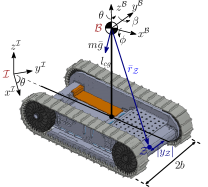
Figure 2: Zero moment point illustration for a mobile robot.

The ZMP is the point on the ground where the gravity and inertia forces create only a non-zero moment about the direction of the plane normal, resulting in zero tipping moment [21]. We compute the mobile robot’s ZMP relative to the ground plane and constrain it so that the vehicle does not tip over. The ZMP-based rollover constraint is given by

$$|y_{\mathcal{Z}}(t)|\leq{b},$$ (29)

where ${y_{\mathcal{Z}}}$ is the lateral component of the ZMP, and $b$ is the half width of the robot. To obtain ${y_{\mathcal{Z}}}$, we model the orientation of the body-fixed frame relative to the fixed world frame via Euler angles ${\phi,\beta,\theta}$, which are called the roll, pitch, and yaw angles, respectively. The vectors representing angular rates, angular accelerations, and linear accelerations are given by ${\bar{\omega}\!=\!\big{[}\dot{\phi}~{}\dot{\beta}~{}\omega\big{]}^{\mathrm{T}};\ \bar{\alpha}\!=\!\big{[}\ddot{\phi}~{}\ddot{\beta}~{}\dot{\omega}\big{]}^{\mathrm{T}};\ \bar{a}\!=\!\big{[}\ddot{x}^{\mathcal{B}}~{}\ddot{y}^{\mathcal{B}}~{}\ddot{z}^{\mathcal{B}}\big{]}^{\mathrm{T}}}$, respectively. The inertia tensor of the robot is given by ${I\!=\!\operatorname{diag}(I_{x},I_{y},I_{z})}$, and $m$ is the total vehicle mass. For the equations of motion in the body frame, we assume the robot is a rigid body, neglecting internal deformations. Assuming zero total forces in the ${y}^{\mathcal{B}}$ and ${z}^{\mathcal{B}}$ directions, as well as zero moments in the ${x}^{\mathcal{B}}$ and ${y}^{\mathcal{B}}$ directions, we have:

$$\ddot{y}^{\mathcal{B}}=-v\!~{}\omega;\quad\ddot{z}^{\mathcal{B}}=0;\quad I_{x}\ddot{\phi}+(I_{y}-I_{z})\dot{\beta}\!~{}\omega=0.$$ (30)

In Fig. 2, $\mathcal{Z}$ is the ZMP point, and ${\bar{r}_{\mathcal{Z}}\!=\![x_{\mathcal{Z}}~{}y_{\mathcal{Z}}~{}\!-\!l_{cg}]^{\mathrm{T}}}$, where $l_{cg}$ is the distance of robot center of mass from the ground. The moment vector about the ZMP is given by

$${M}_{\mathcal{Z}}=(\bar{r}_{\mathcal{Z}}\times m\bar{a})+(\bar{r}_{\mathcal{Z}}\times m\bar{g})+(I\bar{\alpha}+\bar{\omega}\times I\bar{\omega}),$$ (31)

where ${\bar{g}\!=\![g_{x}~{}g_{y}~{}g_{z}]^{\mathrm{T}}}$ is the gravity vector expressed in the body-fixed frame $\mathcal{B}$. From the definition of the ZMP, the moment at the ZMP must satisfy that

$${M}_{\mathcal{Z}}=\begin{bmatrix}0&0&M_{\mathcal{Z}_{z}}\end{bmatrix}^{\mathrm{T}}.$$ (32)

Then solving (31) with (32) yields:

$$y_{\mathcal{Z}}\!=\!\dfrac{-m\ddot{y}^{\mathcal{B}}l_{cg}\!-\!mg_{y}l_{cg}\!-\!(I_{x}\ddot{\phi}\!+\!(I_{y}\!-\!I_{z})\dot{\beta}\!~{}\omega)}{m\ddot{z}^{\mathcal{B}}+mg_{z}},$$ (33)

and substituting (30) into (33) yields:

$$y_{\mathcal{Z}}\!=\!(v\!~{}\omega\!~{}l_{cg}-g_{y}\!~{}l_{cg})/g_{z}.$$ (34)

From (34) and (29) we obtain two different time-dependent safety constraints:

$$\begin{split}h_{1}(t,x)&=v\!~{}\omega-{b}/{l_{cg}}\!~{}{g_{z}}(t)-g_{y}(t)\geq 0\\ h_{2}(t,x)&=-v\!~{}\omega-{b}/{l_{cg}}\!~{}{g_{z}}(t)+g_{y}(t)\geq 0,\end{split}$$ (35)

where ${g_{z},g_{y}}$ are measurable noisy parameters. The function $h_{1}$ represents safety on the right, while $h_{2}$ represents the left.

Remark 3.

With the unicycle model, in which $v$ and $\omega$ are the control inputs, the safety constraints (35) depend on these inputs. Inspired by integral CBFs [22], which generalize control input-dependent CBFs, we extend the unicycle model dynamics with first-order actuator dynamics as given in (28), where ${u_{v},u_{\omega}}$ are the new control inputs.

Problem 1.

Given the system dynamics (28) and the noisy gravity vector measurements ${g_{z},~{}\!g_{y}}$, synthesize a rollover preventing controller satisfying (35) for all ${t\!\geq\!0}$, while ensuring robustness against the disturbance input $d$.

IV-B Experimental Validation

We now apply our formal results to an experiment on an unmanned ground mobile robot. For the test vehicle and onboard computation details, see Section IV in [23]. We conducted experimental tests on an approximately 27^∘ inclined surface, which can cause tipover.

To solve Problem 1, we first designed a controller ${\mathbf{k_{d}}}$:

$$\mathbf{k_{d}}(x)=\begin{bmatrix}K_{v}d_{g}&K_{\omega}{y_{g}-y^{\mathcal{I}}}/{d_{g}}-K_{\omega}\sin{\theta}\end{bmatrix}^{\mathrm{T}},$$

where ${K_{v},\!~{}K_{\omega}}$ are the controller gains, ${x_{g},\!~{}y_{g}}$ are the goal position of the robot, and ${d_{g}\!\triangleq\!\|x_{g}\!-\!x^{\mathcal{I}},\!~{}y_{g}\!-\!y^{\mathcal{I}}\|}$. The inputs were constrained such that ${u_{v}\!\in\![-3,3]}$ m/s², and ${u_{\omega}\!\in\![-2,2]}$ rad/s². The goal position ${x_{g},\!~{}y_{g}}$ is chosen to yield a violation of the safety constraint when using the desired controller. The control loops were realized at 50 Hz loop rate. The differentiator (19) is used to differentiate ${g_{z}}$ and ${g_{y}}$.

The results of the experiments are presented in Fig 1. The figure illustrates that the proposed method assures the safety of the uncertain system by filtering the unsafe desired controller through the derived CBFs.

V Conclusion

This study developed a rollover prevention method for mobile robots using CBFs and ZMP-based safety measures. A robust safety-critical controller was proposed, incorporating the ISS differentiator dynamics and the notion of PSSf. Experiments conducted on a tracked robot demonstrated the effectiveness of the method in preventing rollover.

References

- [1] V. S. Medeiros, E. Jelavic, M. Bjelonic, R. Siegwart, M. A. Meggiolaro, and M. Hutter, “Trajectory optimization for wheeled-legged quadrupedal robots driving in challenging terrain,” IEEE Robot. Autom. Lett., vol. 5, no. 3, pp. 4172–4179, 2020.
- [2] S.-Y. Jeon, R. Chung, and D. Lee, “Planned trajectory classification for wheeled mobile robots to prevent rollover and slip,” IEEE Robot. Autom. Lett., 2023.
- [3] P. R. Roan, A. Burmeister, A. Rahimi, K. Holz, and D. Hooper, “Real-world validation of three tipover algorithms for mobile robots,” in 2010 IEEE Int. Conf. Robot. Autom. IEEE, 2010, pp. 4431–4436.
- [4] Y. D. Viragh, M. Bjelonic, C. D. Bellicoso, F. Jenelten, and M. Hutter, “Trajectory optimization for wheeled-legged quadrupedal robots using linearized zmp constraints,” IEEE Robot. Autom. Lett., vol. 4, no. 2, pp. 1633–1640, 2019.
- [5] J. Song, A. Petraki, B. J. DeHart, and I. Sharf, “Chance-constrained rollover-free manipulation planning with uncertain payload mass,” IEEE/ASME Trans. Mechatronics, 2023.
- [6] S. Lee, M. Leibold, M. Buss, and F. C. Park, “Rollover prevention of mobile manipulators using invariance control and recursive analytic ZMP gradients,” Adv. Robot., vol. 26, no. 11-12, pp. 1317–1341, 2012.
- [7] A. D. Ames, X. Xu, J. W. Grizzle, and P. Tabuada, “Control barrier function based quadratic programs for safety critical systems,” IEEE Trans. Autom. Control, vol. 62, no. 8, pp. 3861–3876, 2017.
- [8] K. P. W. et al., “Data-driven safety filters: Hamilton-Jacobi reachability, control barrier functions, and predictive methods for uncertain systems,” IEEE Control Syst. Mag., vol. 43, no. 5, pp. 137–177, 2023.
- [9] A. J. Taylor, A. Singletary, Y. Yue, and A. D. Ames, “A control barrier perspective on episodic learning via projection-to-state safety,” IEEE Control Syst. Lett., vol. 5, no. 3, pp. 1019–1024, 2020.
- [10] S. Kolathaya and A. D. Ames, “Input-to-state safety with control barrier functions,” IEEE Control Syst. Lett., vol. 3, no. 1, pp. 108–113, 2018.
- [11] T. G. Molnar, A. K. Kiss, A. D. Ames, and G. Orosz, “Safety-critical control with input delay in dynamic environment,” arXiv preprint arXiv:2112.08445, 2021.
- [12] I. Tezuka and H. Nakamura, “Time-varying obstacle avoidance by using high-gain observer and input-to-state constraint safe control barrier function,” IFAC-PapersOnLine, vol. 53, no. 5, pp. 391–396, 2020.
- [13] J. L. Daleckii and M. G. Krein, Stability of solutions of differential equations in Banach space. American Mathematical Soc., Providence, RI, USA, 1974.
- [14] E. Daş and R. M. Murray, “Robust safe control synthesis with disturbance observer-based control barrier functions,” in IEEE Conf. Decision and Control. IEEE, 2022, pp. 5566–5573.
- [15] F. Blanchini and S. Miani, Set-theoretic methods in control. Springer, 2008, vol. 78.
- [16] R. Seeber, H. Haimovich, M. Horn, L. M. Fridman, and H. De Battista, “Robust exact differentiators with predefined convergence time,” Automatica, vol. 134, p. 109858, 2021.
- [17] H. K. Khalil and L. Praly, “High-gain observers in nonlinear feedback control,” Int. J. Robust and Nonlinear Control, vol. 24, no. 6, pp. 993–1015, 2014.
- [18] D. Astolfi, L. Marconi, L. Praly, and A. R. Teel, “Low-power peaking-free high-gain observers,” Automatica, vol. 98, pp. 169–179, 2018.
- [19] D. R. Agrawal and D. Panagou, “Safe and robust observer-controller synthesis using control barrier functions,” IEEE Control Syst. Lett., vol. 7, pp. 127–132, 2022.
- [20] A. I. Mourikis, N. Trawny, S. I. Roumeliotis, D. M. Helmick, and L. Matthies, “Autonomous stair climbing for tracked vehicles,” Int. J. Robotics Res., vol. 26, no. 7, pp. 737–758, 2007.
- [21] P. Sardain and G. Bessonnet, “Forces acting on a biped robot. Center of pressure-zero moment point,” IEEE Trans. Syst. Man Cybern. A: Syst. Hum., vol. 34, no. 5, pp. 630–637, 2004.
- [22] A. D. Ames, G. Notomista, Y. Wardi, and M. Egerstedt, “Integral control barrier functions for dynamically defined control laws,” IEEE Control Syst. Lett., vol. 5, no. 3, pp. 887–892, 2020.
- [23] N. C. Janwani, E. Daş, T. Touma, S. X. Wei, T. G. Molnar, and J. W. Burdick, “A learning-based framework for safe human-robot collaboration with multiple backup control barrier functions,” arXiv preprint arXiv:2310.05865, 2023.