Strategizing against Q-learners: A Control-theoretical Approach

Abstract

In this paper, we explore the susceptibility of the Q-learning algorithm (a classical and widely used reinforcement learning method) to strategic manipulation of sophisticated opponents in games. We quantify how much a strategically sophisticated agent can exploit a naive Q-learner if she knows the opponent’s Q-learning algorithm. To this end, we formulate the strategic actor’s problem as a Markov decision process (with a continuum state space encompassing all possible Q-values) as if the Q-learning algorithm is the underlying dynamical system. We also present a quantization-based approximation scheme to tackle the continuum state space and analyze its performance both analytically and numerically.

1 Introduction

The widespread adoption of (reinforcement) learning algorithms in multi-agent systems has significantly enhanced autonomous systems to tackle complex tasks through learning from interactions within a shared environment. However, strategically sophisticated actors can exploit such algorithms to perform sub-optimally (Huang and Zhu, 2019, 2021; Deng et al., 2019; Vundurthy et al., 2023; Dong and Mu, 2022). A critical question is how much a strategically sophisticated agent can exploit the opponent’s learning dynamics for more payoff if the agent is aware of the opponent’s learning dynamic. This strategic act can also have a positive impact on the naive agent depending on how aligned their objectives are.

To address the challenge, we approach the problem from a control-theoretical perspective. We focus on the repeated play of general-sum normal-form games played by two agents: Alice and Bob. Bob naively follows the widely-used Q-learning algorithm as if Alice is a part of the underlying environment and acts according to some stationary strategy. On the other hand, Alice is a strategically sophisticated agent aware of Bob’s Q-learning algorithm. We show that Alice can leverage this knowledge to control/drive Bob’s algorithm (as if the algorithm is some dynamical system) to maximize the discounted sum of the payoffs collected over an infinite horizon by converting the problem to a Markov decision process (MDP). However, the MDP has a continuum state space. To address this issue, we also present a quantization-based approximation scheme reducing the problem to a finite MDP that can be solved via standard dynamic programming methods. We quantify the approximation level of this scheme and examine its performance numerically.

Learning algorithms relying on feedback from the environment (such as Q-learning) can be vulnerable to exploitation through the manipulation of the feedback by some adversaries. For example, Huang and Zhu (2019, 2021) investigate the impact of manipulating Q-learners through the falsification of cost signals and its effect on the algorithm’s convergence. Correspondingly, robust variants of the Q-learning against such attacks have been studied extensively (Sahoo and Vamvoudakis, 2020; Nisioti et al., 2021; Wang et al., 2020).

Apart from such vulnerabilities, Q-learning dynamics can also lead to peculiar outcomes in the game settings by leading to tacit collusion that can undermine the competitive nature of the markets (Calvano et al., 2020; Klein, 2021; Hansen et al., 2021; Banchio and Mantegazza, 2022). For example, Banchio and Mantegazza (2022) study the collusive behavior of Q-learners in the widely-studied prisoner’s dilemma game (where agents have two actions: ‘cooperate’ and ‘deflect’). They observe that Q-learners can learn to collude in cooperation even though ‘cooperate’ is always an irrational choice as ‘deflect’ dominates ‘cooperate’ strategy. New regulations are needed to prevent such collusive behavior (Calvano et al., 2020). Here, we study the susceptibility of Q-learners against strategic actors. Such vulnerabilities can incentivize businesses not to use Q-learning with the hope of tacit collusion as their naive approach might be exploited by the other business with strategically sophisticated algorithms.

Strategizing against naive learning algorithms has been studied for no-regret learning and fictitious play dynamics (Deng et al., 2019; Dong and Mu, 2022; Vundurthy et al., 2023). Deng et al. (2019) show that sophisticated agents can secure the Stackelberg equilibrium value against no-regret learners. Dong and Mu (2022) study strategizing against a fictitious player in two-agent games with two actions. Vundurthy et al. (2023) prove that sophisticated agents with the knowledge of game matrix can attain better payoffs than the one at Nash equilibrium by solving a linear program for each action of the fictitious player to obtain her own mixed strategy, then play a pure action trajectory to satisfy the desired mixed strategy probabilities. On the other hand, here, we focus on strategizing against the widely-studied Q-learning algorithms and bringing the problem to the control-theoretical framework.

The paper is organized as follows: We formulate the strategic actor’s MDP problem in Section 2. We present the quantization-based approximation scheme in Section 3. We provide illustrative examples and conclude the paper, resp., in Sections 4 and 5. Three appendices include the proofs of technical lemmas.

2 Strategic Actors against Q-Learners

Consider a normal-form game $\mathcal{G}$ played by Alice and Bob. We can characterize this game by the tuple $\langle A,B,u,\overline{u}\rangle$, where $A$ and $B$ denote their finite action sets and $u:A\times B\rightarrow\mathbb{R}$ and $\overline{u}:A\times B\rightarrow\mathbb{R}$ denote their payoff functions respectively. Alice and Bob are repeatedly playing this game over stages $k=0,1,\ldots$.

Bob is a Q-learner who naively follows the Q-learning algorithm. Given his q-function denoted by $q_{k}:B\rightarrow\mathbb{R}$ at stage $k$, he responds according to the softmax function:

$$\sigma(q_{k})(b)=\frac{\exp(q_{k}(b)/\tau)}{\displaystyle\sum_{\tilde{b}\in B}\exp(q_{k}(\tilde{b})/\tau)}\quad\forall b\in B,$$ (1)

for some $\tau>0$ controlling the level of exploration and $\sigma(q_{k})(b)\in(0,1]$ denotes the probability that he takes action $b\in B$. Let $a_{k}\in A$ and $b_{k}\in B$ denote the actions of Alice and Bob at stage $k$, respectively. Given the payoff $\overline{u}_{k}=\overline{u}(a_{k},b_{k})$ he receives, Bob updates his q-function according to

$$q_{k+1}(b)=\begin{cases}q_{k}(b)+\alpha(\overline{u}_{k}-q_{k}(b))&\;\text{if }b=b_{k}\\ q_{k}(b)&\;\text{o.w}\end{cases},$$ (2)

with some step size $\alpha\in(0,1)$ and the initial vector $q_{0}(b)=0$ for all $b$.

On the other hand, Alice is a strategic actor who is aware that Bob is naively following the Q-learning algorithm (2). She can leverage this knowledge to maximize the discounted sum of payoffs she can collect over the infinite horizon, as formulated in the following problem.

Problem 1 (Main Problem) Alice’s goal is to solve,

$$\max_{\{a_{k}\}_{k=1}^{\infty}}\mathrm{E}\left[\sum_{k=0}^{\infty}\gamma^{k}u(a_{k},b_{k})\right],$$ (3)

where the expectation is taken with respect to the randomness on her action $a_{k}$ and Bob’s action $b_{k}\sim\sigma(q_{k})$ while $q_{k}$ is evolving according to (2) and $\gamma\in(0,1)$ is some discount factor.

To solve (3), Alice can take actions according to some decision function $\pi_{k}\in\Delta(A)$, i.e., $a_{k}\sim\pi_{k}$, depending on her observations $\{a_{0},b_{0},\ldots,a_{k-1},b_{k-1}\}$ up to stage $k$ and the knowledge that $q_{k}$ evolves according to (2). We highlight that the information set grows unboundedly. However, Bob’s action depends only on his q-function. Therefore, Alice can reformulate Problem 2 as the following MDP problem whose state is Bob’s q-function.

Problem 2 (MDP Formulation) Consider an MDP characterized by the tuple $\mathcal{M}=\langle Q,A,r,p,\gamma\rangle$, where $Q\subset\mathbb{R}^{|B|}$ is the compact set of states (corresponding to all possible q-vectors), $A$ is the finite set of actions as in $\mathcal{G}$, the reward function $r:Q\times A\rightarrow\mathbb{R}$ is given by

$$r(q,a)=\mathrm{E}_{b\sim\sigma{(q)}}[u(a,b)]$$ (4)

and $p(\cdot|\cdot)$ is the transition kernel for the q-function evolving according to (2). For example, given $(q,a)\in Q\times A$, the state $q$ can only transit to $q_{+}\in Q$ for which $q_{+}(b)=(1-\alpha)q(b)+\alpha\cdot\overline{u}(a,b)$ and $q_{+}(b^{\prime})=q(b^{\prime})$ for all $b^{\prime}\neq b$ for some $b\in B$. The transition probability is given by

$$p(q_{+}\mid q,a)=\sigma(q)(b)$$ (5)

and the softmax function $\sigma(\cdot)$ is as described in (1). The discount factor $\gamma\in(0,1)$ is as described in Problem 2. Then, Alice’s goal can be written as

$$\max_{\{a_{k}\}_{k=1}^{\infty}}\mathrm{E}\left[\sum_{k=0}^{\infty}\gamma^{k}r(q_{k},a_{k})\right],$$ (6)

where the expectation is taken with respect to the randomness on $(q_{k},a_{k})$.

If Alice had access to Bob’s q-function, i.e., the underlying state of the MDP in Problem 2, then the history vector $\{q_{0},a_{0},\ldots,q_{k-1},a_{k-1},q_{k}\}$ of Problem 2 would have been a sufficient statistic for Problem 2 since any history vector $\{a_{0},b_{0},\ldots,a_{k-1},b_{k-1}\}$ of Problem 2 is a function of the history vector of Problem 2. Correspondingly, Alice could have focused on solving Problem 2 without any loss of generality. However, Alice does not observe Bob’s q-function $q_{k}$. Therefore, Alice cannot directly apply the dynamic programming methods to solve Problem 2.

As Alice and Bob take actions simultaneously, Alice can observe/recall Bob’s (previous) action $b_{k-1}$ taken according to the (previous) q-function $q_{k-1}$, i.e., $b_{k-1}\sim\sigma(q_{k-1})$. Therefore, Alice faces an MDP with one-stage delayed partial/noisy observations. Alice can overcome the incomplete state information by converting Problem 2 to a fully observed MDP on some belief space $\mathcal{P}(Q)$ as a standard solution. Here, $\mathcal{P}(Q)$ denotes the space of probability measures on $(Q,\mathcal{B}(Q))$ and $\mathcal{B}(Q)$ is the Borel $\sigma$-algebra on $Q\subset\mathbb{R}^{|B|}$. Define the belief-state by

$$Z_{k}(\cdot):=\Pr(q_{k}\in\cdot\mid b_{0},\ldots,b_{k-1},a_{0},\ldots,a_{k-1})\in\mathcal{P}(Q).$$ (7)

Then, we can define the belief-MDP accordingly. However, Alice knows that Bob is following (2). Therefore, the belief-state $Z_{k}$ corresponds to the point-mass $\delta_{q_{k}}\in\mathcal{P}(Q)$ at $q_{k}\in Q$ and Alice can track the underlying state of the MDP perfectly by using a state observer as if she has direct access to Bob’s q-function. We leave the study of the cases where Alice knows Bob’s algorithm imperfectly such that the belief-MDP does not necessarily match with Problem 2 as an interesting future research direction.

The following proposition characterizes the optimal decision rule for the MDP $\mathcal{M}$ with continuum state space.

Proposition 1. There exists an optimal stationary policy (a stochastic kernel on $A$ given $Q$) for $\mathcal{M}$.

Proof. The proof follows from (Puterman, 2014, Theorem 6.2.12) based on the observation that the set of all possible q-vectors, $Q$, is a Polish space as a compact subset of $\mathbb{R}^{|B|}$ and the set of actions, $A$, is finite and state-invariant. $\square$

We emphasize that the state space $Q$ is not finite and Alice is not able to apply the dynamic programming methods to Problem 2 directly even with the perfect state observer. The following section addresses how Alice can solve Problem 2 through approximation.

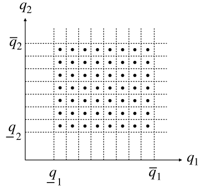
Figure 1: An illustration of the (point-mass) quantization scheme for $Q=[\underline{q}_{1},\overline{q}_{1}]\times[\underline{q}_{2},\overline{q}_{2}]\subset\mathbb{R}^{2}$, where the scalars $\underline{q}_{i}$ and $\overline{q}_{i}$ denote the lower and upper bounds on the $i$th entries of the q-vectors. The quantizer $\Phi:Q\rightarrow D$ maps each q-vector within a cell (the set $Q_{d}$) to a single value $d$ represented by a dot within the cell, i.e., $d\in Q_{d}$, and $D$ is the finite set of these dots.

3 APPROXIMATION

We focus on the quantization-based approximation to reduce Problem 2, with continuum state space $Q\subset\mathbb{R}^{|B|}$, to an MDP with finite state space $D\subset Q$, e.g., see (Saldi et al., 2018). To this end, we consider a quantization mapping $\Phi:Q\rightarrow D$ such that $Q_{d}:=\{q\in Q:\Phi(q)=d\}$ satisfies $Q_{d}\cap Q_{d^{\prime}}=\varnothing$ for all $d\neq d^{\prime}$ and $\bigcup_{d\in D}Q_{d}=Q$, as illustrated in Figure 1. Note that the quantization-based approximation is relatively easier to implement for Problem 2 since $Q$, the space of all possible q-vectors, corresponds to the product space of finite intervals, i.e., $Q=\bigtimes_{i=1}^{|B|}[\underline{q}_{i},\overline{q}_{i}]$ for some scalars $\underline{q}_{i}$ and $\overline{q}_{i}$. Then, Alice faces the following finite MDP.

Problem 3 (Approximation) Consider an MDP characterized by the tuple $\mathcal{A}=\langle D,A,r_{D},\rho,\gamma\rangle$, where $D\subset Q$ is the finite range space of the quantizer $\Phi:Q\rightarrow D$, the finite action set $A$ is as described in $\mathcal{G}$, the reward function $r_{D}:D\rightarrow\mathbb{R}$ is the restriction of $r$, as described in (4), to the set $D$ (i.e., $r_{D}(d,a)=r(d,a)$ for all $d\in D$), the transition probabilities $\rho(\cdot|\cdot)$ are defined by

$$\rho(d_{+}\mid d,a)=\int_{Q_{d_{+}}}p(dq_{+}\mid d,a),$$ (8)

where the transition kernel $p(\cdot|\cdot)$ is as described in Problem 2, and $\gamma\in(0,1)$ is the discount factor from Problem 2. Then, Alice’s goal is now to solve

$$\max_{\{a_{k}\}_{k=0}^{\infty}}\mathbb{E}\left[\sum_{k=0}^{\infty}\gamma^{k}r_{D}(d_{k},a_{k})\right],$$ (9)

where $d_{k}$ is the quantized state at stage $k$, i.e., $d_{k}=\Phi(q_{k})$.

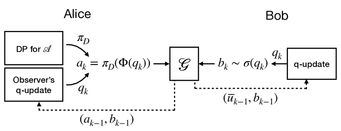
Figure 2: An illustration of how Alice and Bob take actions in the repeated play of $\mathcal{G}$. The dashed lines represent the observations from the previous stage.

Given the q-function $q(\cdot)$ and the action profile $(a,b)$, we denote the next q-function by

$$q_{+}^{ab}(b^{\prime}):=\left\{\begin{array}[]{ll}(1-\alpha)\cdot q(b)+\alpha\cdot\overline{u}(a,b)&\mbox{if }b^{\prime}=b\\ q(b^{\prime})&\mbox{if }b^{\prime}\neq b\end{array}\right.$$ (10)

Then, the q-update (2) yields that (8) can also be written as

$$\rho(d_{+}\mid q,a)=\sum_{\stackrel{{\scriptstyle b\in B:}}{{\Phi(q_{+}^{ab})=d_{+}}}}\sigma(q)(b)\quad\forall q\in D.$$ (11)

Based on (11), Alice can directly compute the transition probabilities for the MDP $\mathcal{A}$ and solve it to find her best decision rule $\pi_{D}:D\rightarrow A$ via dynamic programming, e.g., backward induction, rather straightforwardly. Then, she takes her actions $a_{k}$ according to the decision rule computed and the q-function tracked via the state-observer while Bob is naively playing according to the Q-learning algorithm, as illustrated in Figure 2.

Next, we quantify the performance of the quantization-based approximation scheme in terms of its quantization level. To this end, we introduce the value functions $v_{\kappa}:Q\rightarrow\mathbb{R}$ and $\widehat{v}_{\kappa}:Q\rightarrow\mathbb{R}$, corresponding to the values of the states in $Q$ at the initial stage of a $(\kappa+1)$-length horizon for the best decision rules, resp., in $\mathcal{M}$ and $\mathcal{A}$. More explicitly, for each $q\in Q$, we have

$$v_{\kappa}(q)=\max_{a\in A}\left\{r(q,a)+\gamma\int_{Q}v_{\kappa-1}(\tilde{q})p(d\tilde{q}\mid q,a)\right\}$$ (12)

for all $\kappa>0$ and $v_{0}(q)=\max_{a\in A}\left\{r(q,a)\right\}$. Similarly, for each $q\in Q$, we have

$$\widehat{v}_{\kappa}(q)=\max_{a\in A}\left\{r(\Phi(q),a)+\gamma\int_{Q}\widehat{v}_{\kappa-1}(\tilde{q})p(d\tilde{q}\mid\Phi(q),a)\right\}$$ (13)

for all $\kappa>0$ and $\widehat{v}_{0}(q)=\max_{a\in A}\left\{r(\Phi(q),a)\right\}$. Note that $\widehat{v}_{\kappa}(q)=\widehat{v}_{\kappa}(q^{\prime})$ if $\Phi(q)=\Phi(q^{\prime})$.

Theorem 1. Given the quantization mapping $\Phi$, assume that there exists $\Delta<0$ such that $\|q-\Phi(q)\|_{2}\leq\Delta$ for all $q\in Q$. Then, we have

$$\|v_{\kappa}-\widehat{v}_{\kappa}\|_{\infty}\leq\frac{\Delta\sqrt{|B|}}{\tau(1-\gamma)^{3}}\max_{a,b}|u(a,b)|\quad\forall\kappa\geq 0,$$ (14)

where $v_{\kappa}$ and $\widehat{v}_{\kappa}$ are, resp., as described in (12) and (13).

Proof. We first focus on the case $\kappa=0$. By the definitions of $v_{0}$ and $\widehat{v}_{0}$, we have

$$|v_{0}(q)-\widehat{v}_{0}(q)| =\left|\max_{a}\{r(q,a)\}-\max_{a}\{r(\Phi(q),a)\}\right|$$

$$\leq\max_{a}\left|r(q,a)-r(\Phi(q),a)\right|$$ (15)

where the inequality is due to the non-expansiveness of the maximum function. Then, we can use the following lemma showing the Lipschitz continuity of the reward function.

Lemma 1. The reward function $r(q,a)$ is Lipschitz continuous in $q\in Q$. For each $a\in A$, we have

$$|r(q,a)-r(\overline{q},a)|\leq L_{0}\|q-\overline{q}\|_{2}\quad\forall q,\overline{q}\in Q,$$ (16)

where $L_{0}:=\frac{1}{\tau}\sqrt{|B|}\max_{a,b}|u(a,b)|$.

Based on Lemma 2, (15) yields that

$$|v_{0}(q)-\widehat{v}_{0}(q)|\leq L_{0}\|q-\Phi(q)\|_{2}\quad\forall q\in Q.$$ (17)

Next, we focus on $\kappa>0$. Based on the definitions of $v_{\kappa}$ and $\widehat{v}_{\kappa}$, resp., as described in (12) and (13), the non-expansiveness of the maximum function and the triangle inequality yield that

$$|v_{\kappa}(q)-\widehat{v}_{\kappa}(q)|\leq\max_{a}|r(q,a)-r(\Phi(q),a)|+\gamma\max_{a}\left|\int_{Q}v_{\kappa-1}(\tilde{q})p(d\tilde{q}\mid q,a)-\int_{Q}\widehat{v}_{\kappa-1}(\tilde{q})p(d\tilde{q}\mid\Phi(q),a)\right|.$$

We can bound the first term on the right-hand side by using Lemma 2. Therefore, we focus on the second term. However, in the second term, not only the integrands $v_{\kappa-1}$ and $\widehat{v}_{\kappa-1}$ but also the measures $p(\cdot\mid q,a)$ and $p(\cdot\mid\Phi(q),a)$ are different. To address this issue, we can add and subtract the term $\int_{Q}v_{\kappa-1}(\tilde{q})p(d\tilde{q}\mid\Phi(q),a)$. Then, by the triangle inequality, we have

$$\left|\int_{Q}v_{\kappa-1}(\tilde{q})p(d\tilde{q}\mid q,a)-\int_{Q}\widehat{v}_{\kappa-1}(\tilde{q})p(d\tilde{q}\mid\Phi(q),a)\right|$$

$$\hskip 14.45377pt\leq\left|\int_{Q}v_{\kappa-1}(\tilde{q})p(d\tilde{q}\mid q,a)-\int_{Q}v_{\kappa-1}(\tilde{q})p(d\tilde{q}\mid\Phi(q),a)\right|$$

$$\hskip 28.90755pt+\left|\int_{Q}(v_{\kappa-1}(\tilde{q})-\widehat{v}_{\kappa-1}(\tilde{q}))p(d\tilde{q}\mid\Phi(q),a)\right|.$$ (18)

To bound the first term on the right-hand side of (18), we can use the following lemma showing the Lipschitz continuity of certain linear functionals of the transition kernel $p(\cdot|\cdot)$.

Lemma 2. Let $\eta:Q\rightarrow\mathbb{R}$ be bounded $|\eta(q)|\leq M$ for all $q\in Q$ and $K$-Lipschitz with respect to $\|\cdot\|_{2}$. Then we have

$$\left|\int_{Q}\eta(\tilde{q})p(d\tilde{q}|q,a)-\int_{Q}\eta(\tilde{q})p(d\tilde{q}|\overline{q},a)\right|\leq\overline{K}\|q-\overline{q}\|_{2},$$ (19)

where $\overline{K}=K+\frac{\sqrt{|B|}}{\tau}\cdot M$.

However, Lemma 2 is for bounded Lipschitz continuous functions. The following lemma shows the boundedness and Lipschitz continuity of $v_{\kappa}(\cdot)$ so that we can invoke Lemma 2 for $v_{\kappa}(\cdot)$.

Lemma 3. The value function $|v_{\kappa}(q)|\leq M_{\kappa}$, where

$$M_{\kappa}:=\frac{1-\gamma^{\kappa+1}}{1-\gamma}\max_{(a,b)}|u(a,b)|$$

for all $q\in Q$ and $\kappa\geq 0$. The value function is also $L_{\kappa}$-Lipschitz with respect to $\|\cdot\|_{2}$, where

$$L_{\kappa}=\gamma L_{\kappa-1}+L_{0}\frac{1-\gamma^{\kappa+1}}{1-\gamma}$$

for all $\kappa>0$ and $L_{0}$ is as described in Lemma 2.

Based on Lemma 2, we can invoke Lemma 2 to bound the first term on the right-hand side of (18) by

$$\left|\int_{Q}v_{\kappa-1}(\tilde{q})p(d\tilde{q}\mid q,a)-\int_{Q}v_{\kappa-1}(\tilde{q})p(d\tilde{q}\mid\Phi(q),a)\right| \leq\left(L_{\kappa-1}+\frac{\sqrt{|B|}}{\tau}M_{\kappa-1}\right)\|q-\Phi(q)\|_{2}$$

$$=\left(L_{\kappa-1}+L_{0}\frac{1-\gamma^{\kappa}}{1-\gamma}\right)\|q-\Phi(q)\|_{2},$$ (20)

where the equality follows from the definitions of $L_{0}$ and $M_{\kappa-1}$. On the other hand, we can bound the second term on the right-hand side of (18) by

$$\left|\int_{Q}(v_{\kappa-1}(\tilde{q})-\widehat{v}_{\kappa-1}(\tilde{q}))p(d\tilde{q}\mid\Phi(q),a)\right|\leq\|v_{\kappa-1}-\widehat{v}_{\kappa-1}\|_{\infty},$$ (21)

Then, by Lemma 2 and the bounds (20), (21), we obtain

$$|{v}_{\kappa}(q)-\widehat{v}_{\kappa}(q)| \leq\left(L_{0}+\gamma L_{\kappa-1}+\gamma L_{0}\frac{1-\gamma^{\kappa}}{1-\gamma}\right)\|q-\Phi(q)\|_{2}+\gamma\|v_{\kappa-1}-\widehat{v}_{\kappa-1}\|_{\infty}$$

$$=L_{\kappa}\cdot\|q-\Phi(q)\|_{2}+\gamma\|v_{\kappa-1}-\widehat{v}_{\kappa-1}\|_{\infty}.$$ (22)

Given $\Delta\geq\|q-\Phi(q)\|_{2}$ for all $q$, we have

$$\|v_{0}-\widehat{v}_{0}\|_{\infty}\leq L_{0}\cdot\Delta$$ (23a)

$$\|{v}_{\kappa}-\widehat{v}_{\kappa}\|_{\infty}\leq L_{\kappa}\cdot\Delta+\gamma\|v_{\kappa-1}-\widehat{v}_{\kappa-1}\|_{\infty}\quad\forall\kappa>0$$ (23b)

The recursion (23) on $\|v_{\kappa}-\widehat{v}_{\kappa}\|_{\infty}$ implies that

$$\|v_{\kappa}-\widehat{v}_{\kappa}\|_{\infty}\leq\Delta\cdot\sum_{k=0}^{\kappa}\gamma^{\kappa-k}L_{k}.$$ (24)

On the other hand, the recursion on $\{L_{\kappa}\}_{\kappa\geq 0}$ (as described in Lemma 2) implies that

$$L_{\kappa}=L_{0}\sum_{\ell=0}^{\kappa}(\ell+1)\gamma^{\ell}.$$ (25)

After some algebra, (24) and (25) yield (14). $\square$

4 Illustrative Examples

Lastly, we examine the performance of the strategic actor in the widely-studied matching pennies (MP) and prisoner’s dilemma (PD) games. In the MP, agents have actions: Head (H) and Tail (T). Row player (aiming matches) has the game matrix $U_{1}:=\begin{bmatrix}1&-1\\ -1&1\end{bmatrix}$ whereas the column player (aiming mismatches) has the game matrix $\overline{U}_{1}=-U_{1}$. In the MP, there are no dominated strategies and no pure-strategy equilibrium. The only equilibrium is when both agent play each action with equal probabilities. In the PD, agents have actions: Cooperate (C) and Deflect (D). Row player has the game matrix $U_{2}:=\begin{bmatrix}0.5&-1\\ 1&-0.5\end{bmatrix}$ whereas the column player has the game matrix $\overline{U}_{2}=U_{2}^{T}$. In the PD, ‘C’ is dominated by ‘D’ and the only equilibrium is when both agent deflect.

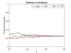
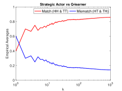
\begin{overpic}[width=130.08731pt,keepaspectratio]{policy_MP.eps} \put(30.0,50.0){{\color[rgb]{1,1,0}H}} \put(70.0,25.0){{\color[rgb]{0,0,1}T}} \end{overpic}

(a) Matching Pennies

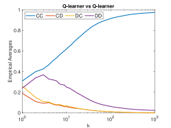
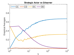
\begin{overpic}[width=130.08731pt,keepaspectratio]{policy_PD.eps} \put(25.0,55.0){{\color[rgb]{0,0,1}C}} \put(60.0,35.0){{\color[rgb]{0,0,1}C}} \put(50.0,50.0){{\color[rgb]{0,0,1}D}} \put(49.0,52.0){\color[rgb]{0,0,1}\vector(-1,0){6.0}} \end{overpic}

(b) Prisoner’s Dilemma

Figure 3: The evolution of the empirical averages of the action profiles for Q-learner vs Q-learner (on the left-most plots) and strategic actor vs Q-learner (on the middle plots) for the matching pennies and prisoner’s dilemma games. The right-most plots show Alice’s decision rule for the quantized q-function, as in Figure 1. There blue and yellow, resp., refer to “H” and “T” (and “C” and “D”) in the matching pennies (and prisoner’s dilemma) games.

We examine the evolutions of the empirical averages of the action profiles in both MP and PD. We set the parameters of the Q-learning algorithms as $\tau=0.01$ and $\alpha=0.05$. We set $\gamma=0.95$ for the MDP problem. We quantize the first and second entries of the q-function to $1000$ uniform intervals over $[-1,1]$ and $[-1,1]$ in the MP (and $[-1,0.5]$ and $[-0.5,1]$ in the PD). We run $100$ independent trials and present the mean empirical average of the action profiles in both Q-learner vs Q-learner and strategic actor vs Q-learner scenarios for both MP and PD in Figure 3. We also demonstrate Alice’s decision rule depending on Bob’s quantized q-function.

Q-learners reach mixed-strategy equilibrium in the MP and their utilities (i.e., discounted sums of the payoffs normalized by $1-\gamma$ for $10^{3}$ iterations) are zero. On the other hand, they learn to collude in ‘CC’ in PD and their utilities are around $0.30$. However, the strategic actors can exploit the Q-learners in both games. In the MP, actions match more frequently (80% of the time) and the strategic actor gets the utility of $0.5$ while the Q-learner gets $-0.5$. Similarly, in the PD, strategic actor can occasionally deflect against always cooperating Q-learner (around 30% of the time) and gets the utility of $0.45$ while the Q-learner gets zero.

5 Conclusion

We addressed how a strategically sophisticated agent can strategize against a naive opponent following Q-learning if the strategic actor knows the opponent’s algorithm and the underlying game payoffs. We approached the problem from a control-theoretical perspective as if the opponent’s Q-learning algorithm is some dynamical system. We modeled the strategic actor’s objective as an MDP problem in which the underlying state corresponds to the opponent’s Q-function. However, this resulted in an MDP with a continuum state space. We presented a quantization-based approximation to reduce the problem to a finite MDP that can be solved via dynamic programming. We also analytically quantified the approximation level and numerically examined the quantization scheme’s performance.

This work paves the way for understanding the vulnerabilities of learning algorithms against strategic actors from a control-theoretical perspective so that we can design algorithms used in the wild reliably. Possible research directions include (i) understanding the vulnerabilities of other widely used algorithms, (ii) reducing the capabilities of the strategic actor, and (iii) using other approximation methods.

Appendix A Proof of Lemma 2

By (4), the left-hand side of (16) can be written as

$$|u(a,\cdot)^{T}(\sigma(q)-\sigma(\overline{q}))| \stackrel{{\scriptstyle(a)}}{{\leq}}\|u(a,\cdot)\|_{2}\|\sigma(q)-\sigma(\overline{q})\|_{2}$$

$$\stackrel{{\scriptstyle(b)}}{{\leq}}L_{0}\|q-\overline{q}\|_{2},$$ (26)

where $(a)$ follows from the Cauchy-Schwartz inequality, and $(b)$ follows from the definition of $\|\cdot\|_{2}$ and $\frac{1}{\tau}$-Lipschitz continuity of the softmax function $\sigma(\cdot)$ with respect to $\|\cdot\|_{2}$, e.g., see (Gao and Pavel, 2017, Proposition 4).

Appendix B Proof of Lemma 2

By the definition of the transition kernel $p(\cdot|\cdot)$, as described in Problem 2, we can write the left-hand side of the inequality (19) as

$$\Xi:=\left|\sum_{b}\sigma(q)(b)\cdot\eta(q_{+}^{ab})-\sum_{b}\sigma(\overline{q})(b)\cdot\eta(\overline{q}_{+}^{ab})\right|,$$ (27)

where $q_{+}^{ab}$, as described in (10), is the next q-function given the q-function $q(\cdot)$ and the action profile $(a,b)$. Correspondingly, $\overline{q}_{+}^{ab}$ is the next q-function given the quantized q-function $\Phi(q)$ and the action profile $(a,b)$.

If we add and subtract $\sum_{b}\sigma(q)(b)\cdot\eta(\overline{q}_{+}^{ab})$, the triangle inequality yields that $\Xi\leq\Xi_{1}+\Xi_{2}$, where

$$\Xi_{1}\coloneqq\left|\sum_{b}\sigma(q)(b)\cdot\left(\eta(q_{+}^{ab})-\eta(\overline{q}_{+}^{ab})\right)\right|,$$ (28a)

$$\Xi_{2}\coloneqq\left|\sum_{b}\Big{(}\sigma(q)(b)-\sigma(\overline{q})(b)\Big{)}\cdot\eta(\overline{q}_{+}^{ab})\right|.$$ (28b)

Then, we can bound $\Xi_{1}$ by

$$\Xi_{1} \stackrel{{\scriptstyle(a)}}{{\leq}}K\sum_{b}\sigma(q)(b)\cdot\|q_{+}^{ab}-\overline{q}_{+}^{ab}\|_{2}$$

$$\stackrel{{\scriptstyle(b)}}{{\leq}}K\|q-\overline{q}\|_{2},$$ (29)

where $(a)$ follows from the $K$-Lipschitz continuity of $\eta(\cdot)$ from the statement of the lemma, and $(b)$ follows from $\|\sigma(q)\|_{1}=1$ and the fact that

$$\|q_{+}^{ab}-\overline{q}_{+}^{ab}\|_{2}^{2} =(1-\alpha)^{2}|q(b)-\overline{q}(b)|^{2}+\sum_{b^{\prime}\neq b}|q(b^{\prime})-\overline{q}(b^{\prime})|^{2}$$

$$\leq\|q-\overline{q}\|_{2}^{2}.$$ (30)

On the other hand, we can bound $\Xi_{2}$ by

$$\Xi_{2} \stackrel{{\scriptstyle(a)}}{{\leq}}\|\sigma(q)-\sigma(\overline{q})\|_{2}\left(\sum_{b}|\eta(\overline{q}_{+}^{ab})|^{2}\right)^{1/2}$$

$$\stackrel{{\scriptstyle(b)}}{{\leq}}\frac{1}{\tau}\sqrt{|B|}M\|q-\overline{q}\|_{2}.$$ (31)

where $(a)$ follows from the Cauchy-Schwarz inequality and $(b)$ follows from the $1/\tau$-Lipschitz continuity of the softmax function and the boundedness of $\eta(\cdot)$ from the statement of the lemma. Combining (29) and (31) lead to (19).

Appendix C Proof of Lemma 2

The first part of the proof follows from the definitions (4) and (12) since we can bound $v_{\kappa}(\cdot)$ by

$$|v_{\kappa}(q)| \leq\sum_{k=0}^{\kappa}\gamma^{k}\max_{(q,a)}|r(q,a)|$$

$$\leq\sum_{k=0}^{\kappa}\gamma^{k}\max_{(a,b)}|u(a,b)|$$

$$\leq\frac{1-\gamma^{\kappa+1}}{1-\gamma}\max_{(a,b)}|u(a,b)|=:M_{\kappa}$$ (32)

The second part of the proof follows from induction. Firstly, for $\kappa=0$, the non-expansiveness of the maximum function leads to

$$|v_{0}(q)-v_{0}(\overline{q})| \leq\max_{a}|r(q,a)-r(\overline{q},a)|$$

$$\leq L_{0}\|q-\overline{q}\|_{2},$$ (33)

where the last inequality is due to Lemma 2. Next, we focus on $\kappa>0$ and assume that $v_{\kappa-1}(\cdot)$ is $L_{\kappa-1}$-Lipschitz with respect to $\|\cdot\|_{2}$. The non-expansiveness of the maximum function and the triangle inequality yield that

$$|v_{\kappa}(q)-v_{\kappa}(\overline{q})|\leq\max_{a}|r(q,a)-r(\overline{q},a)|+\gamma\max_{a}\left|\int_{Q}v_{\kappa-1}(\tilde{q})p(d\tilde{q}|q,a)-\int_{Q}v_{\kappa-1}(\tilde{q})p(d\tilde{q}|\overline{q},a)\right|.$$

For the first term on the right-hand side, we can again invoke Lemma 2. On the other hand, for the second term, we can invoke Lemma 2 based on (32) and the assumption that $v_{\kappa-1}$ is $L_{\kappa-1}$-Lipschitz to obtain

$$|v_{\kappa}(q)-v_{\kappa}(\overline{q})| \leq\left(L_{0}+\gamma\left(L_{\kappa-1}+\frac{\sqrt{|B|}}{\tau}M_{\kappa-1}\right)\right)\|q-\overline{q}\|_{2}$$

$$=\left(L_{0}\sum_{\ell=0}^{\kappa}\gamma^{\ell}+\gamma L_{\kappa-1}\right)\|q-\overline{q}\|_{2}\quad\forall q,\overline{q}\in Q,$$ (34)

where the equality follows from the definition of $L_{0}$ and $M_{\kappa-1}$. This completes the proof.

References

- Banchio and Mantegazza [2022] Martino Banchio and Giacomo Mantegazza. Adaptive algorithms and collusion via coupling. arXiv preprint arXiv:2202.05946, 2022.
- Calvano et al. [2020] Emilio Calvano, Giacomo Calzolari, Vincenzo Denicolo, and Sergio Pastorello. Artificial intelligence, algorithmic pricing, and collusion. American Economic Review, 110(10):3267–3297, 2020.
- Deng et al. [2019] Yuan Deng, Jon Schneider, and Balasubramanian Sivan. Strategizing against no-regret learners. In Advances in Neural Information Processing Systems (NeurIPS), volume 32, 2019.
- Dong and Mu [2022] Hongcheng Dong and Yifen Mu. The optimal strategy against fictitious play in infinitely repeated games. In Proceedings of the 41st Chinese Control Conference (CCC), 2022.
- Gao and Pavel [2017] Bolin Gao and Lacra Pavel. On the properties of the softmax function with application in game theory and reinforcement learning. arXiv preprint arXiv:1704.00805, 2017.
- Hansen et al. [2021] Karsten T Hansen, Kanishka Misra, and Mallesh M Pai. Frontiers: Algorithmic collusion: Supra-competitive prices via independent algorithms. Marketing Science, 40(1):1–12, 2021.
- Huang and Zhu [2019] Yunhan Huang and Quanyan Zhu. Deceptive reinforcement learning under adversarial manipulations on cost signals. In T. Alpcan, Y. Vorobeychik, J. Baras, and G. Dan, editors, International Conference on Decision and Game Theory for Security, volume 11836 of Lecture Notes in Computer Science. Springer, Cham., 2019.
- Huang and Zhu [2021] Yunhan Huang and Quanyan Zhu. Manipulating reinforcement learning: Stealthy attacks on cost signals. In Game Theory and Machine Learning for Cyber Security, pages 367–388. John Wiley & Sons, 2021.
- Klein [2021] Timo Klein. Autonomous algorithmic collusion: Q-learning under sequential pricing. The RAND Journal of Economics, 52(3):538–558, 2021.
- Nisioti et al. [2021] Eleni Nisioti, Daan Bloembergen, and Michael Kaisers. Robust multi-agent Q-learning in cooperative games with adversaries. In Proceedings of the AAAI Conference on Artificial Intelligence, volume 2, 2021.
- Puterman [2014] Martin L Puterman. Markov decision processes: discrete stochastic dynamic programming. John Wiley & Sons, 2014.
- Sahoo and Vamvoudakis [2020] Prachi Pratyusha Sahoo and Kyriakos G Vamvoudakis. On-off adversarially robust Q-learning. IEEE Control Systems Letters, 4(3):749–754, 2020.
- Saldi et al. [2018] Naci Saldi, Tamás Linder, and Serdar Yüksel. Finite Approximations in discrete-time stochastic control. Springer, 2018.
- Vundurthy et al. [2023] Bhaskar Vundurthy, Aris Kanellopoulos, Vijay Gupta, and Kyriakos G Vamvoudakis. Intelligent players in a fictitious play framework. IEEE Transactions on Automatic Control, 2023.
- Wang et al. [2020] Jingkang Wang, Yang Liu, and Bo Li. Reinforcement learning with perturbed rewards. In Proceedings of the AAAI Conference on Artificial Intelligence, volume 34, 2020.