A Framework for Strategic Discovery of Credible Neural Network Surrogate Models under Uncertainty

Abstract

The widespread integration of deep neural networks in developing data-driven surrogate models for high-fidelity simulations of complex physical systems highlights the critical necessity for robust uncertainty quantification techniques and credibility assessment methodologies, ensuring the reliable deployment of surrogate models in consequential decision-making. This study presents the Occam Plausibility Algorithm for surrogate models (OPAL-surrogate), providing a systematic framework to uncover predictive neural network-based surrogate models within the large space of potential models, including various neural network classes and choices of architecture and hyperparameters. The framework is grounded in hierarchical Bayesian inferences and employs model validation tests to evaluate the credibility and prediction reliability of the surrogate models under uncertainty. Leveraging these principles, OPAL-surrogate introduces a systematic and efficient strategy for balancing the trade-off between model complexity, accuracy, and prediction uncertainty. The effectiveness of OPAL-surrogate is demonstrated through two modeling problems, including the deformation of porous materials for building insulation and turbulent combustion flow for ablation of solid fuels within hybrid rocket motors.

[inst1]organization=Department of Mechanical and Aerospace Engineering,
University at Buffalo,city=Buffalo, state=NY, country=USA

[inst2]organization=Sandia National Laboratories,city=Albuquerque, state=NM, country=USA

1 Introduction

The remarkable advancements in scientific machine learning (SciML) techniques, specifically deep neural networks, ignited an extraordinary revolution in the creation of data-driven surrogate models. These models aim to approximate solutions of high-fidelity physics-based scientific simulations and unlock the potential for computational predictions at significantly lower costs. Going beyond the enabler of once-computationally prohibitive outer-loop challenges such as uncertainty quantification, e.g., [1, 2, 3], Bayesian inference, e.g., [4, 5], design under uncertainty [6], digital twins, e.g., [7, 8, 9, 10, 11], and optimal experimental design, e.g., [12, 13] for complex physical systems, neural network-based surrogate models hold transformative potential in reshaping the formulation and resolution of scientific problems across diverse domains of science, engineering, and medicine.

Despite notable advancements, applying machine learning techniques – originally designed for large data regimes in domains like image processing, computer vision, and natural language processing – encounters significant challenges when directly utilized to construct and establish trust in surrogate models. These obstacles emerge from the inherent spatiotemporal sparsity, limitation, and incompleteness of the scientific data extracted from high-fidelity physical simulations. This intrinsic uncertainty presents substantial challenges to the credibility and prediction reliability of neural network-based surrogate models, as highlighted in works such as [14, 15, 16, 17]. The importance of verification, validation, and uncertainty quantification (VVUQ) for physics-based models against experimental measurements is well-established [18, 19, 20, 21]. However, as SciML becomes increasingly integrated and deployed into high-consequence decision-making for complex physical systems, there arises a critical need for even more robust UQ techniques and rigorous methodologies to assess the credibility of neural network-based surrogate models. In particular, the first shortcoming lies in the common training approach, based on maximum likelihood parameter estimation, which limits neural networks’ robustness against data uncertainty (i.e., adversarial attack), resulting in overfitting and overconfident predictions. The second challenge stems from the existing validation methodologies for neural networks, such as train-and-test approaches that rely on empirical performance assessments with asymptotic guarantees in large data [22, 23, 14]. Moreover, the interpretability and explainability approaches employed by the machine learning community to build trust in neural network models often resort to heuristic and problem-dependent strategies [14, 16, 17]. The third and perhaps most pivotal challenge lies in the uncertainty associated with selecting the surrogate model itself. Achieving a delicate balance in the model’s complexity is crucial, as overly simplistic models may compromise predictive ability, while excessively complex ones are prone to overfitting the training data, resulting in poor generalization, especially when parameters are estimated via maximum likelihood methods [24, 25, 21]. Consequently, determining the “best” neural network model becomes challenging in the absence of predefined rules for network architecture and associated hyperparameters Current trial-and-error architecture selection approaches based on testing data performance are time-consuming and resource-intensive and may not effectively enhance the accuracy and reliability of the surrogate models. Harnessing recent advancements in architecture optimization algorithms and software tools [26, 27, 28, 29, 30, 31, 32], when adapted to align the objectives of surrogate modeling, holds the potential to address this challenge effectively.

The Bayesian framework is the cornerstone for successful VVUQ methods, allowing the quantification of uncertainty in model parameters and choice of the model itself in small data regimes, e.g., [33, 34, 35, 36, 5, 37, 38, 39, 40] and serving as a robust foundation for validating model predictions, e.g., [18, 19, 21, 20, 41, 42]. The seminal contributions of Mackay et al. [43, 24] laid the groundwork for the adoption of the Bayesian framework in inferring neural network parameters and hyperparameters, inspiring subsequent developments [44, 25]. Despite these early contributions, Bayesian neural networks (BayesNN) only recently gained recognition in the SciML community, e.g., [45, 46, 47, 2, 48, 49, 50, 51, 49]. The delayed adoption can be attributed to the incomplete understanding of UQ methods for neural networks as well as the computational complexities associated with high-dimensional parameter spaces in these models. BayesNN provides remarkable advantages, including alleviating overfitting, preventing overconfident parameter estimation in small and uncertain datasets, and the ability to quantify prediction uncertainty. This study emphasizes an additional benefit of BayesNN in surrogate modeling by relaxing rigid constraints on model complexity. This flexibility enables the retention of a sufficient number of parameters, crucial for capturing the underlying multiscale structure inherent in physics-based simulations. Despite these merits, BayesNN surrogate modeling faces formidable challenges, particularly in (i) selecting a specific network architecture and hyperparameters, as it is challenging to assert that the chosen models align with prior beliefs about the problem, and (ii) developing methodologies to rigorously assess the credibility and prediction reliability of the surrogate models under uncertainty.

This contribution introduces the Occam Plausibility Algorithm for surrogate models (OPAL-surrogate), a systematic framework designed to discover predictive neural network-based surrogate models for high-fidelity physical simulations. The name is inspired by the principle of Occam’s Razor, advocating the preference for simpler models over unnecessary complex ones, guided by the notion of model plausibility as a basis for its effectiveness in explaining the given data. OPAL-surrogate is grounded in hierarchical Bayesian inferences, enabling a systematic determination of the probability distributions of the network parameters and hyperparameters and measures for comparing various neural network models. Moreover, it adheres to the principles of Bayesian model validation to assess the credibility and prediction reliability of the surrogate model. Leveraging these methodologies, OPAL-surrogate presents a strategy to adaptively adjust model complexity, utilizing a combination of bottom-up and top-down approaches until predefined validation criteria are met. Consequently, within the wide space of potential BayesNN models, involving choices of architecture and hyperparameters, OPAL-surrogate identifies the “best” predictive surrogate model by balancing the trade-off between model complexity, accuracy, and prediction uncertainty. The effectiveness of OPAL-surrogate is demonstrated via two modeling problems in solid mechanics and computational fluid dynamics, identifying credible surrogate models for reliable prediction of quantities of interest (QoIs).

Following this introduction, Section 2 provides a comprehensive overview of Bayesian learning for neural networks and an efficient and scalable solution algorithm. Section 3 delves into the definition of the BayesNN model and hierarchical inference of various classes of neural network parameters. The steps involved in the OPAL-surrogate for discovering BayesNN surrogate models are outlined in Section 4. Section 5 shows numerical examples, including the identification of BayesNN surrogate models for the elastic deformation of porous materials with random microstructures and the direct numerical simulation of turbulent combustion flow for shear-induced ablation of solid fuels within hybrid rocket motors. Concluding remarks can be found in Section 6.

2 Neural Networks Learning as Probabilistic Inference

A neural network is a nonlinear map $\boldsymbol{g}:\mathbb{R}^{d_{i}}\rightarrow\mathbb{R}^{d_{o}}$ from the inputs $\boldsymbol{x}\in\mathbb{R}^{d_{i}}$ to the outputs $\boldsymbol{u}_{\boldsymbol{\theta}}\in\mathbb{R}^{d_{o}}$, representing a continuously parameterized function. The functional form of a feed-forward neural network with $D$ number of layers is expressed as follows,

$$\boldsymbol{u}_{\boldsymbol{\theta}}(\boldsymbol{x})=f^{(D)}(\boldsymbol{w}^{(D)}\cdots f^{(2)}(\boldsymbol{w}^{(2)}f^{(1)}(\boldsymbol{w}^{(1)}\boldsymbol{x}+\boldsymbol{b}^{(1)})+\boldsymbol{b}^{(2)})\cdots+\boldsymbol{b}^{(D)}).$$ (1)

Here, $\boldsymbol{w}^{(\ell)}$ represents the weight vector connecting layer ${\ell}-1$ to layer ${\ell}$, $\boldsymbol{b}^{(\ell)}$ denotes the biases in layer ${\ell}$, and $f^{(\ell)}$ denotes activation functions applied element-wise. The set of weights and biases collectively forms the network parameters $\boldsymbol{\theta}\in\mathbb{R}^{P}$, and common activation functions include Hyperbolic Tangent (Tanh), Rectified Linear Unit (ReLU), Leaky Rectified Linear Unit (Leaky ReLU), and Logistic (Sigmoid) functions. The output in each layer $\ell$ can be represented as

$$\boldsymbol{a}^{(\ell)}=\boldsymbol{w}^{(\ell)}\boldsymbol{z}^{(\ell-1)}+\boldsymbol{b}^{(\ell)};\quad\boldsymbol{z}^{(\ell)}=f^{(\ell)}(\boldsymbol{a}^{(\ell)});\quad 1\leq\ell<D,$$ (2)

where $\boldsymbol{a}^{(\ell)}$ is the pre-activation and $\boldsymbol{z}^{(\ell)}$ denotes the activation values.

The neural network training involves adjusting the weights and biases to minimize the discrepancy between the network output and a given dataset $\boldsymbol{D}=\{\boldsymbol{x}_{\boldsymbol{D}}^{j},\boldsymbol{u}_{\boldsymbol{D}}^{j}\}_{j=1}^{N_{D}}$. Standard training based on the maximum likelihood estimate often leads to overconfidence in parameter values, ignoring inherent uncertainty in model predictions due to limited and uncertain data. BayesNN, however, pose training within a Bayesian inference framework [47, 45, 24, 25, 52], considering a probability distribution function (PDF) over network parameters inferred from data using Bayes’ theorem,

$$\pi_{post}(\boldsymbol{\theta}|\boldsymbol{D})=\frac{\pi_{like}(\boldsymbol{D}|\boldsymbol{\theta})\pi_{pr}(\boldsymbol{\theta})}{\pi_{evid}(\boldsymbol{D})}.$$ (3)

Here, $\pi_{post}(\boldsymbol{\theta}|\boldsymbol{D})$ represents the posterior PDF, updating the prior PDF $\pi_{pr}(\boldsymbol{\theta})$ given observational data and the evidence PDF $\pi_{evid}(\boldsymbol{D})$ serves as the normalization factor. Additionally, the likelihood PDF $\pi_{like}(\boldsymbol{D}|\boldsymbol{\theta})$ is derived from a noise model depicting the discrepancy between the data and neural network output. Adhering to the maximum entropy principle with constraints on the mean and variance of parameters, we adopt a Gaussian prior $\pi_{pr}(\boldsymbol{\theta})=\mathcal{N}(\bar{\boldsymbol{\theta}},\boldsymbol{\Gamma}_{pr})$. Unless derived from pre-training or historical datasets, and without loss of generality, we assume $\bar{\boldsymbol{\theta}}=\boldsymbol{0}$ and prior covariance is $\boldsymbol{\Gamma}_{pr}=(\sigma^{\text{pr}})^{2}\mathbf{I}$ where $\sigma^{\text{pr}}$ is the prior hyper-parameter. Additionally, we consider an additive noise model $\boldsymbol{u}_{D}=\boldsymbol{u}_{\boldsymbol{\theta}}(\boldsymbol{x}_{\boldsymbol{D}})+\boldsymbol{\eta}$ where $\boldsymbol{\eta}$ is the total error, including both data uncertainty and network inadequacy in representing the data. Assuming a zero-mean Gaussian distribution for the total error, $\boldsymbol{\eta}\sim\mathcal{N}\left(\mathbf{0},(\sigma^{\text{noise}})^{2}\mathbf{I}\right)$ and considering independent and identically distributed (iid) data, the likelihood PDF is expressed as,

$$\pi_{\rm like}(\boldsymbol{D}|\boldsymbol{\theta})=\prod_{i=1}^{N_{D}}\frac{1}{\sqrt{2\pi}\sigma^{\text{noise}}}\exp\left[-\frac{(\boldsymbol{u}_{\boldsymbol{D}}^{j}-\boldsymbol{u}_{\boldsymbol{\theta}}(\boldsymbol{x}_{\boldsymbol{D}}^{j}))^{2}}{2(\sigma^{\text{noise}})^{2}}\right]$$ (4)

where $\sigma^{\text{noise}}$ is called noise hyper-parameter. A point estimate of the most probable value for the parameter, considering both the observed data and the prior PDFs, is referred to as the Maximum A Posteriori (MAP) estimate such that,

$$\boldsymbol{\theta}_{MAP}=\underset{\boldsymbol{\theta}\in\Theta}{\text{argmax}}\;\pi_{post}(\boldsymbol{\theta}|\boldsymbol{D}).$$ (5)

Finally, having the posterior PDF of the network parameters, the prediction probability of the output is evaluated as,

$$\pi(\boldsymbol{u}_{\boldsymbol{\theta}}|\boldsymbol{x},\boldsymbol{D})=\int\,\pi(\boldsymbol{u}_{\boldsymbol{\theta}}|\boldsymbol{x},\boldsymbol{\theta})\,\pi_{post}(\boldsymbol{\theta}|\boldsymbol{D})\,d\boldsymbol{\theta}.$$ (6)

2.1 Bayesian solution: Laplace approximation to the posterior

Bayesian inference for neural networks poses substantial computational challenges, primarily due to the high-dimensional parameter space (number of weights) and the potential complexity of the posterior distribution geometry. Neal [53, 25] introduced Hamiltonian Monte Carlo (HMC) for BayesNN, a subset of Markov chain Monte Carlo algorithms theoretically yielding the true posterior PDF. However, the drawback of sampling algorithms is the escalating computational costs with the increasing number of parameters, rendering them impractical for large-scale neural networks. To illustrate the proposed framework for BayesNN surrogate modeling in this work, we leverage an efficient Bayesian solution based on Laplace approximation (LA) to the posterior, offering scalability with respect to the parameter dimensions. This section provides an overview of this solution algorithm.

The utilization of LA in the context of BayesNN has roots in seminal works such as [43, 54, 55]. More recently, its computationally efficient application has been extended to larger networks [56, 57, 58]. The underlying concept of this approach involves approximating the intractable posterior distribution by linearizing it around its dominant mode, particularly the MAP estimate in (5). The approximation is derived through the second-order Taylor expansion of the logarithm of the posterior PDF of the network parameters in (3) around $\boldsymbol{\theta}^{MAP}$,

$$\ln\pi_{post}(\boldsymbol{\theta}|\boldsymbol{D})\approx\ln\pi_{post}(\boldsymbol{\theta}|\boldsymbol{D})|_{\boldsymbol{\theta}=\boldsymbol{\theta}_{MAP}}-\frac{1}{2}(\boldsymbol{\theta}-\boldsymbol{\theta}_{MAP})^{T}\boldsymbol{H}(\boldsymbol{\theta}-\boldsymbol{\theta}_{MAP}),$$ (7)

where $\boldsymbol{H}=-\nabla^{2}_{\boldsymbol{\theta}\boldsymbol{\theta}}\ln\pi_{post}(\boldsymbol{\theta}|\boldsymbol{D})|_{\boldsymbol{\theta}=\boldsymbol{\theta}_{MAP}}$ is the positive (semi-)definite Hessian of the negative log-posterior, describing its local curvature at the MAP point. Exponentiating this expression yields,

$$\pi_{post}(\boldsymbol{\theta}|\boldsymbol{D})\approx\frac{1}{Z}\exp\left[-\ln\pi_{post}(\boldsymbol{\theta}|\boldsymbol{D})|_{\boldsymbol{\theta}=\boldsymbol{\theta}_{MAP}}-\frac{1}{2}(\boldsymbol{\theta}-\boldsymbol{\theta}_{MAP})^{T}\boldsymbol{H}(\boldsymbol{\theta}-\boldsymbol{\theta}_{MAP})\right],$$ (8)

where $Z$ is a normalization factor. Applying Laplace’s method to evaluate the normalization factor results in a posterior approximation [57],

$$\pi_{post}(\boldsymbol{\theta}|\boldsymbol{D})\approx\frac{1}{\sqrt{(2\pi)^{P}\det(\boldsymbol{H})}}\exp\left[-\frac{1}{2}(\boldsymbol{\theta}-\boldsymbol{\theta}_{MAP})^{T}\boldsymbol{H}(\boldsymbol{\theta}-\boldsymbol{\theta}_{MAP})\right],$$ (9)

where $P$ is the number of parameters $\boldsymbol{\theta}$. The relation (9) demonstrates that LA approximates the posterior PDF by a multivariate normal distribution $\mathcal{N}(\boldsymbol{\theta}_{MAP},\boldsymbol{\Gamma}_{post})$. The mean of this distribution is the MAP point $\boldsymbol{\theta}_{MAP}$, and the posterior covariance matrix $\boldsymbol{\Gamma}_{post}=\boldsymbol{H}^{-1}$ is given by the inverse of the Hessian matrix evaluated at $\boldsymbol{\theta}_{MAP}$. The MAP estimate for the parameters can be computed by minimizing the negative log-posterior, which can be expressed equivalently through the likelihood and prior PDFs as,

$$\boldsymbol{\theta}_{MAP}=\underset{\boldsymbol{\theta}}{\text{argmin}}\;\{-\ln\pi_{post}(\boldsymbol{\theta}|\boldsymbol{D})\}=\underset{\boldsymbol{\theta}}{\text{argmin}}\;\{-\ln\pi_{like}(\boldsymbol{D}|\boldsymbol{\theta})-\log\pi_{pr}(\boldsymbol{\theta})\}.$$ (10)

The solution to the above optimization problem is analogous to deterministic neural network training with an updated loss function. Furthermore, the posterior covariance can be expressed as,

$$\boldsymbol{\Gamma}_{post}=\boldsymbol{H}^{-1}=\left(\boldsymbol{H}_{lnlike}+\boldsymbol{\Gamma}_{pr}^{-1}\right)^{-1},$$ (11)

where $\boldsymbol{\Gamma}_{pr}$ is the prior covariances, and $\boldsymbol{H}_{lnlike}=-\nabla^{2}_{\boldsymbol{\theta}\boldsymbol{\theta}}\left.\ln\pi_{like}(\boldsymbol{D}|\boldsymbol{\theta})\right|_{\boldsymbol{\theta}=\boldsymbol{\theta}_{MAP}}$ denotes the Hessian of log-likelihood evaluated at MAP point. To this end, the efficient computation of the log-likelihood Hessian is crucial for the calculation of the posterior covariance, as the prior terms are typically straightforward.

2.2 Scalable algorithm via Kronecker-factored Laplace approximation

The computation of the posterior covariance encounters a significant challenge due to the large size of the $\boldsymbol{H}_{lnlike}$ matrix resulting from the high-dimensional parameter space in neural networks. This matrix is often non-diagonal, not guaranteed to be positive semi-definite, and may lack sparsity. To address this challenge and develop a scalable solution algorithm for Bayesian inference, we adopt the Kronecker factored representation of the Hessian proposed by [59, 60]. This approach takes advantage of the structure of neural network parameters, allowing for explicit calculation, inversion, and storage of the Hessian matrix in a tractable manner. Recent applications of this method in Bayesian neural network inference solutions have also been demonstrated by [56, 61, 62, 58, 57].

Due to the intractability of the $\boldsymbol{H}_{lnlike}\in\mathbb{R}^{P\times P}$, it is common practice to resort to its generalized Gauss-Newton approximation. The resulting symmetric positive and semi-definite approximated Hessian matrix is given by,

$$\boldsymbol{H}_{lnlike}\approx\boldsymbol{J}^{T}\boldsymbol{L}\boldsymbol{J},$$ (12)

where the matrix $\boldsymbol{J}\in\mathbb{R}^{N_{D}d_{o}\times P}$ is formed by concatenating $N_{D}$ Jacobian matrices of the network with respect to the parameters $\boldsymbol{j}(\boldsymbol{x}_{\boldsymbol{D}}^{j})=\nabla_{\boldsymbol{\theta}}\boldsymbol{u}_{\boldsymbol{\theta}}(\boldsymbol{x}_{\boldsymbol{D}}^{j})|_{\boldsymbol{\theta}=\boldsymbol{\theta}_{MAP}}$ $\in\mathbb{R}^{d_{o}\times P}$ for all $\{\boldsymbol{x}_{\boldsymbol{D}}^{j}\}_{j=1}^{N_{D}}$ in the data set, and $\boldsymbol{L}\in\mathbb{R}^{N_{D}d_{o}\times N_{D}d_{o}}$ is a block-diagonal matrix with blocks $\boldsymbol{l}(\boldsymbol{u}_{\boldsymbol{D}}^{j},\boldsymbol{u}_{\boldsymbol{\theta}}(\boldsymbol{x}_{\boldsymbol{D}}^{j}))=-\nabla^{2}_{\boldsymbol{g}\boldsymbol{g}}\ln\pi_{like}(\boldsymbol{D}|\boldsymbol{\theta})|_{\boldsymbol{\theta}=\boldsymbol{\theta}_{MAP}}\in\mathbb{R}^{d_{o}\times d_{o}}$. Despite the approximation in (12), the log-likelihood Hessian remains a full matrix that needs to be inverted. To address the associated computational challenge, we employ a block-diagonal approximation in which the $\boldsymbol{H}_{lnlike}$ matrix is divided into blocks, each corresponding to all weights of one layer of the network. This approach neglects covariance between layers but retains covariance within each layer. We further leverage the Kronecker factored representation of the layer-wise Hessian, denoted as $\boldsymbol{H}_{lnlike}^{(\ell)}$. Proposed by [59, 60], the Kronecker-factored approximation relies on the insight that, for a single data point, the approximation in (12) can be precisely expressed as the Kronecker product of two smaller matrices. To facilitate tractability, the [59, 60] propose approximating the sum of Kronecker products over all data points by a Kronecker product of sums. Consequently, the approximated log-likelihood Hessian for the $\ell$-th layer of the neural network can be represented as,

$$[\boldsymbol{J}^{T}\boldsymbol{L}\boldsymbol{J}]^{(\ell)}\approx\boldsymbol{Q}^{(\ell)}\otimes\boldsymbol{R}^{(\ell)},$$ (13)

where $\boldsymbol{Q}^{(\ell)}=\boldsymbol{z}^{(\ell-1)}(\boldsymbol{z}^{(\ell-1)})^{T}$ is the uncentered covariance of the activations and $\boldsymbol{R}^{(\ell)}=-\nabla^{2}_{\boldsymbol{a}^{(\ell)}\boldsymbol{a}^{(\ell)}}\ln\pi_{like}(\boldsymbol{D}|\boldsymbol{\theta})$ and $\boldsymbol{z}^{(\ell)}$ and $\boldsymbol{a}^{(\ell)}$ are the activation values and the pre-activation for layer $\ell$ defined in (2). As detailed in [60], computing $\boldsymbol{R}^{(\ell)}$ involves a recursive procedure that starts at the output layer, followed by backward propagation through the network in a single pass for each data point, and then averaging across all data points. The matrices $\boldsymbol{Q}^{(\ell)}\in\mathbb{R}^{d_{i}^{(\ell)}\times d_{i}^{(\ell)}}$ and $\boldsymbol{R}^{(\ell)}\in\mathbb{R}^{d_{o}^{(\ell)}\times d_{o}^{(\ell)}}$ depends in the dimensionality of the $\ell$-th layer’s input $d_{i}^{(\ell)}$ and output $d_{o}^{(\ell)}$, and both are positive semidefinite. Consequently, the Kronecker-factored approximation offers a significant computational advantage by decomposing the layer-wise log-likelihood Hessian into smaller matrices [58, 56]. By substituting (12) and (13) into (11), the posterior covariance at the $\ell$-th layer is approximated as,

$$\boldsymbol{\Gamma}_{post}^{(\ell)}\approx\left(\boldsymbol{Q}^{(\ell)}\otimes\boldsymbol{R}^{(\ell)}+{\boldsymbol{\Gamma}_{pr}^{(\ell)}}^{-1}\right)^{-1},$$ (14)

while the entire term under inversion does not necessarily allow a Kronecker-factored representation. To preserve a Kronecker factored structure, [56] suggested approximating the posterior covariance by introducing the effect of the prior as damping factors to $\boldsymbol{Q}^{(\ell)}$ and $\boldsymbol{R}^{(\ell)}$. While such dampening is common in optimization methods employing Kronecker-factored Hessian approximations [59], applying it to a posterior approximation artificially increases the posterior concentration. To prevent the introduction of additional approximations that might overshadow the genuine impact of the prior PDF on inference, we utilize the eigendecompositions $\boldsymbol{Q}^{(\ell)}=\boldsymbol{M}_{Q^{(\ell)}}\boldsymbol{\Lambda}_{Q^{(\ell)}}\boldsymbol{M}_{Q^{(\ell)}}^{T}$ and $\boldsymbol{R}^{(\ell)}=\boldsymbol{M}_{R^{(\ell)}}\boldsymbol{\Lambda}_{R^{(\ell)}}\boldsymbol{M}_{R^{(\ell)}}^{T}$. Here, $\boldsymbol{\Lambda}_{Q^{(\ell)}}=\text{diag}(\boldsymbol{q}^{(\ell)})$ and $\boldsymbol{\Lambda}_{R^{(\ell)}}=\text{diag}(\boldsymbol{r}^{(\ell)})$ where $\boldsymbol{q}^{(\ell)}$ and $\boldsymbol{r}^{(\ell)}$ are the non-negative eigenvalues of $\boldsymbol{Q}^{(\ell)}$ and $\boldsymbol{R}^{(\ell)}$, respectively. Substituting the eigendecompositions into (14) and considering the $\ell$-th block-diagonal entry of prior covariance as $\boldsymbol{\Gamma}_{pr}^{(\ell)}=(\sigma^{\text{pr}(\ell)})^{2}\boldsymbol{I}^{(\ell)}$, results in [62],

$$\boldsymbol{\Gamma}_{post}^{(\ell)}\approx\left((\boldsymbol{M}_{Q^{(\ell)}}\otimes\boldsymbol{M}_{R^{(\ell)}})\,(\boldsymbol{\Lambda}_{Q^{(\ell)}}\otimes\boldsymbol{\Lambda}_{R^{(\ell)}}+(\sigma^{\text{pr}(\ell)})^{-2}\boldsymbol{I}^{(\ell)})\,(\boldsymbol{M}_{Q^{(\ell)}}^{T}\otimes\boldsymbol{M}_{R^{(\ell)}}^{T})\right)^{-1},$$ (15)

where $\boldsymbol{I}^{(\ell)}$ is the identity matrix with dimensions corresponding to the number of parameters in the $\ell$-th layer and $\boldsymbol{M}_{Q^{(\ell)}}\otimes\boldsymbol{M}_{R^{(\ell)}}$ constitutes the eigenvectors of $\boldsymbol{Q}^{(\ell)}\otimes\boldsymbol{R}^{(\ell)}$, making it unitary and facilitating the representation of this identity. The LA and approximated posterior covariance via generalized Gauss-Newton and Kronecker-factored approximations, along with the eigendecomposition of the individual Kronecker factors, results in an efficient and scalable algorithm for Bayesian inference of neural networks.

3 Hierarchical Bayesian inferences and model plausibility

3.1 Bayesian neural networks model

We introduce the BayesNN model denoted by the abstract form $M(\boldsymbol{\phi})$. This representation encapsulates not only the network architecture but also the specifications of the prior of the parameters and the noise model utilized for constructing the likelihood. For the purpose of our later discussion on the discovery and credibility assessment of surrogate models, we categorize the BayesNN model parameters $\boldsymbol{\phi}$ into four distinct subsets, as follows:

1) Network parameters $\boldsymbol{\theta}\in\mathbb{R}^{P}$

These encompass the set of weights and biases constituting a BayesNN, represented collectively as,

$$\boldsymbol{\theta}=[\boldsymbol{w}^{(1)},\cdots,\boldsymbol{w}^{(D)},\boldsymbol{b}^{(1)},\cdots,\boldsymbol{b}^{(D)}].$$ (16)

As discussed earlier, the primary objective of BayesNN training is to determine the probability distributions of the network parameters based on data.

2) Inference hyper-parameters $\boldsymbol{\sigma}\in\mathbb{R}^{H}$

These parameters characterize the Bayesian inference setup and stem from the specifications of the prior and likelihood. More precisely, the prior on the weights and biases, denoted as $\pi_{pr}(\boldsymbol{\theta})$, can be parametrized by $\boldsymbol{\sigma}^{\text{pr}}\in\mathbb{R}^{P}$, such as mean and variance of a Gaussian prior. In practice, one may opt for a single prior hyperparameter on all network parameters or consider distinct priors for each class of parameters (weights out of input units, biases of hidden units, and weights and biases of output units) [25, 24]. Additionally, the likelihood function incorporates noise hyper-parameters $\boldsymbol{\sigma}^{\text{noise}}\in\mathbb{R}^{N_{D}}$ arising from the chosen noise model. The inference hyper-parameters are a collection of prior and noise hyper-parameters as,

$$\boldsymbol{\sigma}=[\boldsymbol{\sigma}^{\text{pr}},\boldsymbol{\sigma}^{\text{noise}}].$$ (17)

3) Architecture hyper-parameters $\boldsymbol{\xi}\in\Xi$

These parameters represent the structural and organizational characteristics of the network, specifying the functional mapping between inputs and outputs. In the case of fully connected networks, the architecture hyper-parameters include the number of layers $D$, the number of neurons $W$ and the activation function $f$ in each layer (i.e., the type of non-linearity applied between layers),

$$\boldsymbol{\xi}=[W^{(1)},\cdots,W^{(D)}f^{(1)},\cdots,f^{(D)}].$$ (18)

Here, $D,W\in\mathbb{N}$ and $f\in\mathcal{F}$, where $\mathcal{F}$ denotes the function space adhering to properties expected of neural network activation functions, such as smoothness, continuity, and convexity. For more advanced models, like convolutional neural networks, the space of architecture hyper-parameters expands significantly, including the number and kernel size of convolutions, channels per convolutional layer, and the number of fully-connected layers, affecting the predictive ability of the model, e.g., [63, 29].

4) Solution hyper-parameters $\chi\in\mathbb{R}^{X}$

Another class of parameters pertains to the selection of Bayesian inference solutions, encompassing choices like sampling algorithms and variational inference, along with the particulars of these algorithms, such as learning rate and weight initialization. For the purposes of this work, we place less emphasis on the impact of the solution hyper-parameters on the network prediction ability. Therefore, throughout the remainder of this manuscript, the BayesNN model explicitly defines the functional form of the network as well as the specifications of the likelihood and prior in Bayesian inference.

3.2 Model evidence

A common method for neural network model selection involves assessing their prediction performance on unseen testing datasets. However, this approach has been criticized for potential instability [64], inefficiency in small data regimes [47], and lack of robustness with respect to data uncertainty. In response, we propose a systematic model selection approach based on Bayesian model plausibility, which utilizes the entire dataset to construct and inform the models. Let $M(\boldsymbol{\phi})$ be a BayesNN model with its own set of model parameters $\boldsymbol{\phi}=[\boldsymbol{\theta},\boldsymbol{\sigma},\boldsymbol{\xi}]$. We rewrite the Bayesian inference (3), acknowledging known information on the inference and architecture hyper-parameters,

$$\pi_{post}(\boldsymbol{\theta}|\boldsymbol{D},\boldsymbol{\sigma},\boldsymbol{\xi})=\frac{\pi_{like}(\boldsymbol{D}|\boldsymbol{\theta},\boldsymbol{\sigma},\boldsymbol{\xi})\pi_{pr}(\boldsymbol{\theta}|\boldsymbol{\sigma},\boldsymbol{\xi})}{\pi_{evid}(\boldsymbol{D}|\boldsymbol{\sigma},\boldsymbol{\xi})}.$$ (19)

The denominator of Bayes theorem (19) is the probability of observing data using model $M$, commonly referred to as the evidence PDF,

$$\pi_{evid}(\boldsymbol{D}|\boldsymbol{\sigma},\boldsymbol{\xi})=\int\pi_{like}(\boldsymbol{D}|\boldsymbol{\theta},\boldsymbol{\sigma},\boldsymbol{\xi})\;\pi_{pr}(\boldsymbol{\theta}|\boldsymbol{\sigma},\boldsymbol{\xi})\;d\boldsymbol{\theta}.$$ (20)

In this setting, the evidence transcends its traditional role as a mere normalization factor in classical Bayesian inference, emerging as a crucial element in our model selection rationale. Specifically, when rearranging (3), the logarithm of evidence can be expressed as [65],

$$\ln\left[\pi_{evid}(\mathbf{D}|\boldsymbol{\sigma},\boldsymbol{\xi})\right] = \int\ln\left[\pi_{like}(\boldsymbol{D}|\boldsymbol{\theta},\boldsymbol{\sigma},\boldsymbol{\xi})\right]\pi_{post}(\boldsymbol{\theta}|\boldsymbol{D},\boldsymbol{\sigma},\boldsymbol{\xi})\;d\boldsymbol{\theta}$$ (21)

$$- \int\ln\left(\frac{\pi_{post}(\boldsymbol{\theta}|\boldsymbol{D},\boldsymbol{\sigma},\boldsymbol{\xi})}{\pi_{pr}(\boldsymbol{\theta}|\boldsymbol{\sigma},\boldsymbol{\xi})}\right)\pi_{post}(\boldsymbol{\theta}|\boldsymbol{D},\boldsymbol{\sigma},\boldsymbol{\xi})\;d\boldsymbol{\theta}.$$

Here, the first term represents the posterior mean of the log-likelihood, while the second term denotes the relative entropy between the prior and posterior distributions, quantifying the information gained about the parameters from the data. In essence, the evidence reflects a trade-off between the model fitting the observed data and the extent to which network parameters $\boldsymbol{\theta}_{i}$ are learned from that data. This characteristic renders the evidence a valuable measure for model comparison [20], particularly in BayesNN models, facilitating comparisons between different architectures, noise models, and prior formulations.

3.3 Hierarchical Bayesian inferences

Building upon MacKay’s evidence framework for BayesNN models [24], the following hierarchical Bayesian inferences are postulated, treating the evidence PDF at each level as a new likelihood function for subsequent Bayesian inference:

• Level 1. Infer the network parameters $\boldsymbol{\theta}$,

  $$\pi_{post}(\boldsymbol{\theta}|\boldsymbol{D},\boldsymbol{\sigma},\boldsymbol{\xi})=\frac{\pi_{like}(\boldsymbol{D}|\boldsymbol{\theta},\boldsymbol{\sigma},\boldsymbol{\xi})\,\pi_{pr}(\boldsymbol{\theta}|\boldsymbol{\sigma},\boldsymbol{\xi})}{\pi_{evid}(\boldsymbol{D}|\boldsymbol{\sigma},\boldsymbol{\xi})}.$$ (22)

• Level 2. Infer the inference hyper-parameters $\boldsymbol{\sigma}$,

  $$\pi_{post}(\boldsymbol{\sigma}|\boldsymbol{D},\boldsymbol{\xi})=\frac{\pi_{evid}(\boldsymbol{D}|\boldsymbol{\sigma},\boldsymbol{\xi})\,\pi_{pr}(\boldsymbol{\sigma}|\boldsymbol{\xi})}{\pi_{evid}(\boldsymbol{D}|\boldsymbol{\xi})}.$$ (23)

• Level 3. Infer the archtecture hyper-parameters $\boldsymbol{\xi}$,

  $$\pi_{post}(\boldsymbol{\xi}|\boldsymbol{D})=\frac{\pi_{evid}(\boldsymbol{D}|\boldsymbol{\xi})\,\pi_{pr}(\boldsymbol{\xi})}{\pi_{evid}(\boldsymbol{D})}.$$ (24)

Performing Level 1 in (22) and Level 2 in (23) has been employed for hyperparameter optimization in Gaussian processes [66], which are inherently rooted in a Bayesian learning framework and have recently found application in BayesNN [45]. However, Level 3 for neural network architecture selection has received comparatively less attention. In particular, (24) facilitates the update of the modeler’s prior belief in a BayesNN model $\pi_{pr}(\boldsymbol{\xi})$ based on data, yielding the posterior model plausibility $\rho=\pi_{post}(\boldsymbol{\xi}|\boldsymbol{D})$.

In the hierarchical Bayesian inference of (22) and (23), there may appear to be a contradiction with Bayesian principles, as the prior for network parameters seems to be determined after observing the data. In other words, it might appear that the most probable value of the prior hyperparameters $\boldsymbol{\sigma}^{\rm pr}$ is chosen first, followed by the utilization of the corresponding prior to infer $\boldsymbol{\theta}$. To clarify this apparent sequence, we recognize that the model prediction can be the integration over the ensemble of unknown network and inference hyperparameters collectively defining the prior. The true posterior used for model prediction in (6) is expressed as:

$$\pi_{post}(\boldsymbol{\theta}|\boldsymbol{D},\boldsymbol{\xi}) = \int\pi(\boldsymbol{\theta},\boldsymbol{\sigma}|\boldsymbol{D},\boldsymbol{\xi})\;d\boldsymbol{\sigma}$$ (25)

$$= \int\pi_{post}(\boldsymbol{\theta}|\boldsymbol{D},\boldsymbol{\sigma},\boldsymbol{\xi})\;\pi_{post}(\boldsymbol{\sigma}|\boldsymbol{D},\boldsymbol{\xi})\;d\boldsymbol{\sigma}.$$

This expression suggests that the posterior of $\boldsymbol{\theta}$ is obtained by integrating over the posteriors for all values of $\boldsymbol{\sigma}$, each weighted by the probability of $\boldsymbol{\sigma}$ given the data. This mirrors the concept of Bayesian model averaging, e.g., [67, 68, 47], where predictions from multiple models (i.e., BayesNN with different inference hyperparameters) are combined, considering the associated uncertainty of each model. Considering $\pi_{post}(\boldsymbol{\sigma}|\boldsymbol{D},\boldsymbol{\xi})$ exhibiting a dominant peak at $\boldsymbol{\sigma}_{MAP}$, then the true posterior $\pi_{post}(\boldsymbol{\theta}|\boldsymbol{D},\boldsymbol{\xi})$ will be primarily governed $\pi_{post}(\boldsymbol{\theta}|\boldsymbol{D},\boldsymbol{\sigma},\boldsymbol{\xi})|_{\boldsymbol{\sigma}=\boldsymbol{\sigma}_{MAP}}$. Consequently, we are justified in using the following approximation [43],

$$\pi_{post}(\boldsymbol{\theta}|\boldsymbol{D},\boldsymbol{\xi})\approx\pi_{post}(\boldsymbol{\theta}|\boldsymbol{D},\boldsymbol{\sigma},\boldsymbol{\xi})|_{\boldsymbol{\sigma}=\boldsymbol{\sigma}_{MAP}}.$$ (26)

Therefore, employing only the most probable prior hyperparameter is a valid approximation for posterior evaluation. We note that the Bayesian model averaging can be extended to combine predictions from multiple network architectures, with each model weighted according to its posterior probability based on the data according to (24).

Numerical solution

The solution to hierarchical Bayesian inferences involves a multi-step procedure. Specifically, Level 1 and Level 2 inferences comprise an iterative scheme for the online determination of network parameters and inference hyperparameters. In each step, the network parameters $\boldsymbol{\theta}$ are inferred with fixed values of the inference hyperparameters $\boldsymbol{\sigma}$ using (22). Subsequently, these parameters are utilized to update $\boldsymbol{\sigma}$ as per (23), maximizing the corresponding evidence $\pi_{evid}(\boldsymbol{D}|\boldsymbol{\sigma},\boldsymbol{\xi})$. Upon completion of the network training and hyperparameters inference, the evidence $\pi_{evid}(\boldsymbol{D}|\boldsymbol{\xi})$ is employed to compute posterior model plausibility in Level 3. Using LA to the posterior and the prior and noise model considered in Section 2, the process of network training and hyperparameter determination entails estimating their corresponding MAP estimates and the posterior covariance. The evidence for updating inference hyperparameters is expressed as,

$$\ln\pi_{evid}(\boldsymbol{D}|\sigma^{\text{noise}^{2}},\sigma^{\text{pr}^{2}},\boldsymbol{\xi})\approx\ln\pi_{like}(\boldsymbol{D}|\boldsymbol{\theta},\sigma^{\text{noise}^{2}},\sigma^{\text{pr}^{2}},\boldsymbol{\xi})|_{\boldsymbol{\theta}=\boldsymbol{\theta}_{MAP}}$$

$$+\ln\pi_{pr}(\boldsymbol{\theta}|\sigma^{\text{noise}^{2}},\sigma^{\text{pr}^{2}},\boldsymbol{\xi})|_{\boldsymbol{\theta}=\boldsymbol{\theta}_{MAP}}-\ln\pi_{post}(\boldsymbol{\theta}|\boldsymbol{D},\sigma^{\text{noise}^{2}},\sigma^{\text{pr}^{2}},\boldsymbol{\xi})|_{\boldsymbol{\theta}=\boldsymbol{\theta}_{MAP}}$$

$$=-\frac{1}{2(\sigma^{\text{noise}})^{2}}\sum_{j=1}^{N_{D}}(\boldsymbol{u}_{D}^{j}-\boldsymbol{u}_{\boldsymbol{\theta}_{MAP}}(\boldsymbol{x}_{D}^{j}))^{2}-\frac{N_{D}}{2}\ln(2\pi(\sigma^{\text{noise}})^{2})$$

$$-\frac{1}{2(\sigma^{\text{pr}})^{2}}\|\boldsymbol{\theta}_{MAP}\|^{2}-\frac{N_{D}}{2}\ln(2\pi(\sigma^{\text{pr}})^{2})-\frac{1}{2}\ln\det\left(\frac{1}{2\pi}\boldsymbol{H}\right),$$ (27)

where $\|\cdot\|$ denotes the Euclidean norm. In the absence of prior information on the inference hyperparameters and the non-Gaussian form of likelihood, we adopt a uniform prior for $\ln(\sigma^{\text{pr}^{2}})$ and $\ln(\sigma^{\text{noise}^{2}})$, in accordance with the recommendation of [43, 24]. This prior facilitates exploration across a broad spectrum of hyperparameters and ensures cancellation when comparing different models. The determination of inference hyperparameters in (23) is then formulated as the maximization of the evidence in (3.3). Moreover, utilizing a Gaussian approximation of $\pi_{post}(\ln(\sigma^{\text{noise}^{2}}),\ln(\sigma^{\text{pr}^{2}})|\boldsymbol{D},\boldsymbol{\xi})$, the model evidence for evaluating the posterior model plausibility in Level 3 is expressed as,

$$\ln\pi_{evid}(\boldsymbol{D}|\boldsymbol{\xi}) \approx \pi_{evid}(\boldsymbol{D}|\sigma^{\text{noise}^{2}},\sigma^{\text{pr}^{2}},\boldsymbol{\xi})|_{\sigma^{\text{noise}}=\sigma^{\text{noise}}_{MAP},\;\sigma^{\text{pr}}=\sigma^{\text{pr}}_{MAP}}$$ (28)

$$\pi_{pr}\left(\ln(\sigma^{\text{noise}^{2}}),\ln(\sigma^{\text{pr}^{2}})|\boldsymbol{\xi}\right)|_{\sigma^{\text{noise}}=\sigma^{\text{noise}}_{MAP},\;\sigma^{\text{pr}}=\sigma^{\text{pr}}_{MAP}}$$

$$(\sqrt{2\pi}\sigma_{\ln\sigma^{\text{noise}}})\,(\sqrt{2\pi}\sigma_{\ln\sigma^{\text{pr}}}),$$

where $\sigma^{2}_{\ln\sigma^{\text{noise}}}$ and $\sigma^{2}_{\ln\sigma^{\text{pr}}}$ are the posterior variances of $\ln(\sigma^{\text{noise}^{2}})$ and $\ln(\sigma^{\text{pr}^{2}})$, respectively. Differentiating $\ln\pi_{evid}(\boldsymbol{D}|\sigma^{\text{noise}^{2}},\sigma^{\text{pr}^{2}},\boldsymbol{\xi})$ in (3.3), Mackay [43] showed that these variances can be approximated by,

$$\sigma^{2}_{\ln\sigma^{\text{pr}}}\approx\frac{2}{P-\text{tr}(\mathbf{H}^{-1})/\sigma^{\text{pr}^{2}}_{MAP}},\quad\sigma^{2}_{\ln\sigma^{\text{noise}}}\approx\frac{2}{N_{D}-P+\text{tr}(\mathbf{H}^{-1})/\sigma^{\text{pr}^{2}}_{MAP}}.$$ (29)

In general, the iterative updating of network parameters and inference hyper-parameters, as well as computing model plausibility, is computationally expensive, primarily due to the computation of the determinant of the Hessian in (3.3) and the trace of its inverse in (28) for high-dimensional parameters. However, we leverage the available eigenvalues of the Kronecker-factored matrices described in Section 2.2 for efficient computation of the determinant and trace,

$$\det(\boldsymbol{H})=\prod_{\ell}\prod_{ij}q_{i}^{(\ell)}r_{j}^{(\ell)}+(\sigma^{\text{pr}(\ell)})^{2},\quad\text{tr}(\boldsymbol{H})=\sum_{\ell}\sum_{ij}q_{i}^{(\ell)}r_{j}^{(\ell)}+(\sigma^{\text{pr}(\ell)})^{2}.$$ (30)

4 A Framework for Surrogate Model Discovery

The primary focus of this study is on surrogate modeling, specifically harnessing BayesNN models as low-computational-cost approximations for solutions of high-fidelity physics-based simulations. Beyond addressing uncertainties arising from limited and sparse data in high-fidelity simulations, credible surrogate models must capture the overall hierarchy of interactions across multiple scales inherent in physics-based simulations. We argue that Bayesian training of neural networks is well-suited for this purpose, as it allows for more complex models with an adequate number of weights to capture the multiscale structure of physics-based simulation. This stands in contrast to maximum likelihood training, where an excessive number of parameters may lead to overfitting and compromise the models’ generalization. Despite these merits, challenges persist in surrogate modeling using BayesNN, particularly in identifying the right model within an enormous space of potential architectures and rigorous methodologies for assessing the accuracy and reliability of surrogates under uncertainty.

In formulating the surrogate modeling problem, let $\mathcal{M}$ be a set of different BayesNN models,

$$\mathcal{M}=\Big{\{}M_{1}(\boldsymbol{\phi}_{1}),M_{2}(\boldsymbol{\phi}_{2}),\cdots,M_{K}(\boldsymbol{\phi}_{K})\Big{\}},$$ (31)

where each model $M_{i},\;i=1,2,\cdots,K$ has its own set of model parameters $\boldsymbol{\phi}_{i}=[\boldsymbol{\theta}_{i},\boldsymbol{\sigma}_{i},\boldsymbol{\xi}_{i}]$. The high-fidelity data $\boldsymbol{D}$ is obtained from the scenario $\mathcal{S}$ that encapsulates features of the high-fidelity simulation such as domain, boundary conditions, and spatial location and frequency from which data is gathered. Later we will argue the importance of considering a hierarchy of scenarios to rigorously assess the validity and predictive reliability of surrogate models. The training process for each model involves hierarchical Bayesian inferences (22)-(24), where we recognize known information about the set $\mathcal{M}$ and scenario $\mathcal{S}$ in the probability distributions, i.e., $\pi_{post}(\boldsymbol{\theta}|\boldsymbol{D},\boldsymbol{\sigma},\boldsymbol{\xi},\mathcal{M},\mathcal{S})$. In this context, the denominator of (24) serves to normalize the discrete probability components over the models in the set $\mathcal{M}$,

$$\pi(\boldsymbol{D}|\mathcal{M},\mathcal{S})=\sum_{i=1}^{K}\pi_{evid}(\boldsymbol{D}|\boldsymbol{\xi}_{i},\mathcal{M},\mathcal{S})\pi_{pr}(\boldsymbol{\xi}_{i}|\mathcal{M}),$$ (32)

resulting in $\sum_{i=1}^{K}\rho_{i}=1,$ with $\rho_{i}=\pi_{post}(\boldsymbol{\xi}_{i}|\boldsymbol{D})$. Hence, within the set of competing models in $\mathcal{M}$ and for a given dataset $\boldsymbol{D}$, the model boasting the highest $\rho_{i}$ is deemed the most plausible model [20, 65]. However, the model evidence alone does not ensure the generalizability and prediction reliability of the model, indicating the need for additional steps for credibility assessment and model validation.

4.1 Occam-Plausibility Algorithm for Surrogates

Building on our previous framework for validation and selection of physics-based models [41, 21, 20], we proposed Occam-Plausibility Algorithm for Surrogate models (OPAL-surrogate), a systematic strategy for discovering the simplest (“best”) credible surrogate model shown in Figure 1. The key enabler to overcome the enormous space of potential BayesNN models is adaptive modeling by replacing discrete choices with continuous parameterization. The OPAL-surrogate involves the following steps:

1. Initialization. Construct an initial set of possible surrogate models $\mathcal{M}$ in (31) and acquired training data $\boldsymbol{D}$ from a scanrio $\mathcal{S}^{(s)}$ with setting $s=1$.

2. Occam Categories. Partition the models in $\mathcal{M}$ based on model complexity measures into Occam categories. The simplest models are placed in Category 1, and the most complex models are designated in the last category. We, therefore, produce a collection of subsets,

   $$\hat{\mathcal{M}}^{(l)}=\Big{\{}M_{1}^{l}(\boldsymbol{\phi}_{1}^{l}),M_{2}^{l}(\boldsymbol{\phi}_{2}^{l}),\cdots,M_{K_{l}}^{l}(\boldsymbol{\phi}_{K_{l}}^{l})\Big{\}},\quad l=1,2\cdots,H,$$ (33)

   where $l$ is the category and ${K_{l}}<K$. A commonly used complexity measure is the number of model parameters $\boldsymbol{\phi}$, although other measures can also be considered, especially when implementing OPAL-surrogate to multiple classes of surrogate models. The categorization of models depends on factors such as the size of the initial model set and the available computational resources.

3. Occam Step and Model Plausibility. Start with the first Occam Category, $l=1$, employ $\boldsymbol{D}$ to identify the plausible model in Category $l$, denoted by $M_{I}^{l}(\boldsymbol{\phi}^{l}_{I})$. This process is formalized as,

   $$\boldsymbol{\xi}_{I}^{l}=\underset{\boldsymbol{\xi}_{k}^{l}\in\bar{\Xi}^{l}}{\text{argmax}}\;\{\rho_{k}^{l}\}_{k=1}^{R_{l}},$$ (34)

   where $\rho_{k}^{l}=\pi_{post}(\boldsymbol{\xi}_{k}^{l}|\boldsymbol{D},\hat{\mathcal{M}}^{(l)},\{\mathcal{S}^{(s)}\}_{s=1}^{S})$ represents the Bayesian posterior plausibility for the $k$-th model in the set $\hat{\mathcal{M}}^{(l)}$, given the high-fidelity data $\boldsymbol{D}$ obtained from a collection of scenarios ${\mathcal{S}^{(1)},\cdots,\mathcal{S}^{(S)}}$.

   Except for rare instances like model selection among a limited space of architectures $\bar{\Xi}^{l}$, such as in [58], discrete optimization in (34) that requires Bayesian inference across all possible models to evaluate $\rho_{i}^{l}$, becomes computationally prohibitive. Instead, one can adopt a uniform prior on all (or a subset of) architecture hyper-parameters $\pi_{pr}(\boldsymbol{\xi}_{i}|\hat{\mathcal{M}}^{(l)})$, and employ adaptive modeling by replacing discrete model choices with continuous parameterization. This transformation turns the optimization problem in (34) into a continuous maximization of the evidence $\pi_{evid}(\boldsymbol{D}|\boldsymbol{\xi}_{i},\hat{\mathcal{M}}^{(l)},\{\mathcal{S}^{(s)}\}_{s=1}^{S})$, facilitating efficient model discovery.

   

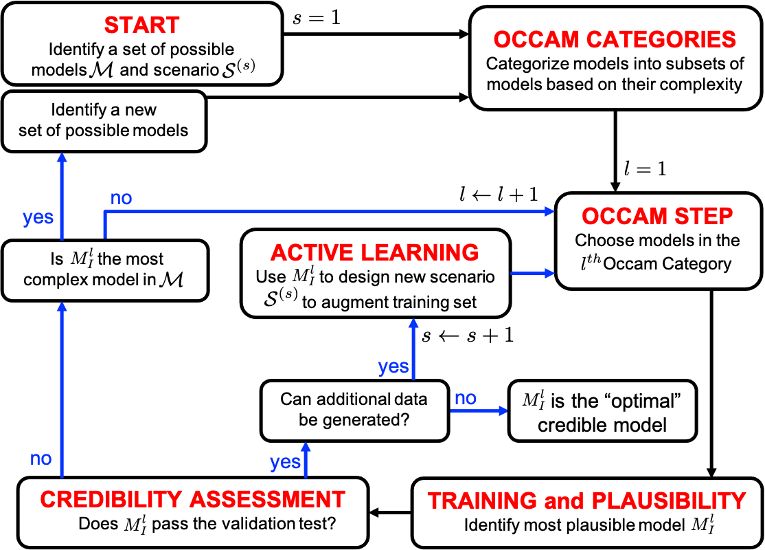
   Figure 1: The Occam Plausibility Algorithm for surrogate models (OPAL-surrogate): Commencing with an initial set of potential models, the models are categorized based on measures of complexity. Starting with the simplest models in the first Occam Category, the most plausible model is determined and undergoes the computationally intensive validation test for credibility assessment. If additional data can be acquired, this validated model guides the design of new scenarios to expand the training set and iteratively re-select new models in response to the updated dataset. The final model that successfully passes the validation test is considered the “best” credible model.

   Solving the possibly non-convex optimization problem using pure machine learning techniques involves leveraging advanced neural architecture search algorithms [26, 27] such as the differential evolution method [28, 29] and software frameworks like Optuna [32] and AutoML [31]. When faced with multiple local maxima due to a small dataset, Bayesian model averaging, e.g., [47], can be employed to combine predictions from various models. However, inspired by [69, 70], our adaptive surrogate modeling takes a distinctive perspective to ensure the BayesNN approximator effectively captures the underlying multiscale structure of the high-fidelity physics-based simulations. To realize this objective, we propose a sequential addition of fully connected layers with sufficiently large widths, guided by the model evidence value, followed by the elimination of irrelevant weights. This strategic approach necessitates an effective network sparsification method to reveal sparsity patterns associated with the inherent multiscale structure encoded in high-fidelity data. One of such methods is described in Section 4.2.

4. Credibility Assessment. Examine the validity of the most plausible model $M_{I}^{l}(\boldsymbol{\phi}^{l}_{I})$, by subjecting it to leave-out cross-validation test. Accordingly, divide the training data $\boldsymbol{D}$ into $N_{v}$ leave-out subsets,

   $$\{\boldsymbol{D}_{LO}^{(n)}\}_{n=1}^{N_{v}}\quad\text{with}\quad\boldsymbol{D}_{LO}^{(n)}=\boldsymbol{D}\setminus\boldsymbol{D}^{(n)}.$$ (35)

   For each subset of data, train $M_{I}^{l}(\boldsymbol{\phi}^{l}_{I})$ with $\boldsymbol{D}^{(n)}$ using the Bayesian inference (22) and (23). Use the posteriors of the network parameters and inference hyper-parameters to evaluate the model output $\boldsymbol{u}_{\boldsymbol{\theta}}(\boldsymbol{x}_{D_{LO}^{(n)}})$ associated with $\boldsymbol{D}_{LO}^{(n)}$. Compare a proper distance measure $\mathbbm{d}(\cdot,\cdot)$ between the model output and the leave-out data set with a given accuracy tolerance $TOL$.

   For $n=1,\cdots,N_{v}$,

   $$\pi_{post}(\boldsymbol{\theta}^{l}_{I}|\boldsymbol{D}^{(n)},\boldsymbol{\sigma}^{l}_{I},\boldsymbol{\xi}^{l}_{I},\hat{\mathcal{M}}^{(l)},\{\mathcal{S}^{(s)}\}_{s=1}^{S})=$$

   $$\frac{\pi_{like}(\boldsymbol{D}^{(n)}|\boldsymbol{\theta}^{l}_{I},\boldsymbol{\sigma}^{l}_{I},\boldsymbol{\xi}^{l}_{I},\hat{\mathcal{M}}^{(l)},\{\mathcal{S}^{(s)}\}_{s=1}^{S})}{\pi_{evid}(\boldsymbol{D}^{(n)}|\boldsymbol{\sigma}^{l}_{I},\boldsymbol{\xi}^{l}_{I},\hat{\mathcal{M}}^{(l)},\{\mathcal{S}^{(s)}\}_{s=1}^{S})}\pi_{pr}(\boldsymbol{\theta}^{l}_{I}|\boldsymbol{\sigma}^{l}_{I},\boldsymbol{\xi}^{l}_{I}),$$

   $$\pi_{post}(\boldsymbol{\sigma}^{l}_{I}|\boldsymbol{D}^{(n)},\boldsymbol{\xi}^{l}_{I},\hat{\mathcal{M}}^{(l)},\{\mathcal{S}^{(s)}\}_{s=1}^{S})=$$

   $$\frac{\pi_{evid}(\boldsymbol{D}^{(n)}|\boldsymbol{\sigma}^{l}_{I},\boldsymbol{\xi}^{l}_{I},\hat{\mathcal{M}}^{(l)},\{\mathcal{S}^{(s)}\}_{s=1}^{S})}{\pi_{evid}(\boldsymbol{D}^{(n)}|\boldsymbol{\xi}^{l}_{I},\hat{\mathcal{M}}^{(l)},\{\mathcal{S}^{(s)}\}_{s=1}^{S})}\pi_{pr}(\boldsymbol{\sigma}^{l}_{I}|\boldsymbol{\xi}^{l}_{I}),$$

   $$\mathbbm{d}^{(n)}\left(\pi(\boldsymbol{u}_{\boldsymbol{D}}(\boldsymbol{x}_{D_{LO}^{(n)}}))\,,\,\pi(\boldsymbol{u}_{\boldsymbol{\theta}}(\boldsymbol{x}_{D_{LO}^{(n)}}))\right)<TOL.$$ (36)

   If the inequality (36)₃ holds for all $N_{v}$, the model $M_{I}^{l}$ is considered as “not invalid” and identified as the best credible surrogate model for the given training data. This designation is made under the recognition that additional data and information could potentially falsify a model initially presumed to be valid. Once the surrogate model is determined, the parameters are updated using the entire training set. This involves substituting $\boldsymbol{D}^{(n)}$ with $\boldsymbol{D}$ in (36)_1,2, and utilizing the inferred network parameters $\pi_{post}(\boldsymbol{\theta}^{l}_{I}|\boldsymbol{D},\boldsymbol{\sigma}^{l}_{I},\boldsymbol{\xi}^{l}_{I},\hat{\mathcal{M}}^{(l)},\{\mathcal{S}^{(s)}\}_{s=1}^{S})$ for making predictions.

5. Scenario Design via Active Learning. If additional computational resources allow for further data generation, the model $M_{I}^{l}(\boldsymbol{\phi}^{l}_{I})$ is utilized to design the next scenario $s\leftarrow s+1$ to augment $\boldsymbol{D}$ with more effective data, following the active learning approach. In cases where surrogate models are utilized for interpolation, this involves leveraging optimal experimental design methods, such as [71, 72, 73], which take a decision-theoretic approach to optimize features of the high-fidelity simulation scenario by maximizing an information gain metric as expected utility. The choice of the utility function depends on the purpose of surrogate modeling and the cost and usefulness of the observational data in a specific problem. However, complications arise in extrapolation when the surrogate model aims to predict unobservable quantities of interest (QoI) beyond the scope of high-fidelity simulation. This poses the formidable challenge of designing a scenario to obtain observational data that reflects the structure of the predicted QoI while ensuring the affordability of the associated high-fidelity simulation [74, 21] and further discussed in Remark 2 below.

6. Iteration and Refinements. If the model $M_{I}^{l}$ is invalid, OPAL returns to the next Occam category $l\leftarrow l+1$ and repeats Steps 3 and 4 until identifying a “not invalid” model and possibly augmenting training data in Step 5. In case all BayesNN models in $\mathcal{M}$ are found to be invalid, it is necessary to enlarge the initial model set.

In the successful execution of OPAL-surrogate, several important considerations merit attention:

Remark 1

While the OPAL-surrogate offers an adaptive strategy for neural network-based surrogate model discovery, it underscores the crucial role of incorporating domain expert knowledge into the modeling process. The effectiveness of this framework hinges on various and often subjective decisions that the modeler must make tailored to a specific problem. These decisions involve defining the initial model set, selecting appropriate complexity measures and effective categorization, establishing the prior distribution for architecture hyper-parameters, setting tolerance and metrics for credibility assessment, and choosing the utility function in scenario design. In the numerical examples presented in Section 5, we will delve into some of these essential features for the implementation of this framework.

Remark 2

A formidable challenge in scientific prediction is the extrapolation beyond the range of available data to predict unobservable QoIs. Section 5 presents a numerical example illustrating this situation, where the surrogate’s objective is to make predictions on a larger domain inaccessible to high-fidelity simulation. The formalization of surrogate modeling, grounded in the concept of a “prediction pyramid” [18, 20], is pivotal in augmenting the reliability of extrapolation predictions. At the base of the prediction pyramid is the pre-training scenario $\mathcal{S}_{c}$, with a lower computational cost of the high-fidelity simulation. It facilitates the generation of a large set of pre-training data $\boldsymbol{D}_{c}$, contributing to establishing a meaningful prior distribution on the network parameters. Ascending the pyramid is the training scenario $\mathcal{S}$, involving more complex high-fidelity simulations that provide training dataset $\boldsymbol{D}$, used to inform and test the surrogate model’s trustworthiness and prediction reliability. At the top of the pyramid is the prediction scenario $\mathcal{S}_{p}$, the most complex scenario where conducting high-fidelity simulation is practically impossible. The surrogate model prediction relies on the extrapolation of training data and the design of a meaningful training scenario that accurately captures the features of the QoIs in the prediction scenario [21, 74].

4.2 Network sparsification strategy

As outlined in Section 4.1, an effective sparsification is needed to ensure the surrogate model captures the inherent multiscale structure within high-fidelity physical simulations. The conventional method involves pruning by setting tentative network parameters to zero, followed by training the new model to accept the pruning based on a performance measure. However, explicitly pruning one parameter at a time becomes computationally prohibitive for large networks [24]. In contrast, we seek to automatically assess the relevance of network parameters, preserving those deemed relevant to enhance the predictive performance of the surrogate model. A suitable category of methods for this purpose is Automatic Relevance Determination (ARD), widely applied in sparse regression [75, 76, 77]. Despite the advantages of ARD over the pruning methods, practical challenges may arise in implementing ARD within BayesNN, as discussed by Mackay and Neal [24, 25]. Notably, dealing with numerous relevance hyperparameters can hinder the calculation of evidence for different models, particularly when handling a large number of network parameters with limited data.

In this work, we advocate exploiting sparsity-enforcing priors to eliminate irrelevant parameters of BayesNN, e.g., [78, 75]. From a Bayesian perspective, such a prior reflects our belief that certain parameters are less likely to be relevant than others. This leads us to anticipate that these parameters will be centered around a specific value, with penalization for deviations from this mode. Employing the maximum entropy principle for constructing prior probability distributions [79], we obtain a Laplace distribution by imposing constraints on both the mean of the network parameters and their absolute deviation (L1 norm) from the mean, expressed as,

$$\pi_{pr}(\boldsymbol{\theta})=\prod_{i=1}^{P}\frac{1}{\beta}\exp\left[-\frac{\left|\theta_{i}-\bar{\theta_{i}}\right|}{\beta}\right],$$ (37)

where $\beta>0$ is the scale parameter. It is worth noting that, Williams [78] justified the use of the Laplace prior by employing a transformation groups approach to prior construction [80]. He exploited a symmetry property inherent in neural network models, asserting the existence of a functionally equivalent network where the weight on a given connection has the same magnitude but opposite sign. This symmetry mandates that the prior for a given weight should depend on its absolute value.

Our proposed network sparsification method involves applying a Laplace prior to the network parameters, followed by magnitude-based thresholding. Parameters with sufficiently small magnitudes, denoted as $|\theta_{i}|<TOL_{\boldsymbol{\theta}}$, are considered irrelevant and subsequently removed from the model. The level of aggressiveness in parameter removal is controlled to maximize the model evidence, achieved by incrementally increasing the threshold $TOL_{\boldsymbol{\theta}}$ until the evidence value of the resulting sparsed network begins to decline. This approach can be regarded as a soft implementation of the sparsification method proposed by Williams [78].

Discovering the category-wise plausible model

We propose the following strategy for implementing Step 3 of OPAL-surrogate across a wide range of possible BayesianNN models. In this context, we characterize fully connected neural network architectures by their depth $D$ (number of layers), width $W$ (number of neurons in each layer), and each layer’s activation function, employing a uniform prior on all architecture hyper-parameters:

1. Within each Occam category, identify a fully connected network architecture with the smallest depth and largest width. Among different choices of activation functions for the layer, select the one that yields the highest evidence $\pi_{evid}(\boldsymbol{D}|\boldsymbol{\xi}_{(\cdot)}^{l},\hat{\mathcal{M}}^{l},\mathcal{S})$.

2. Sequentially add a fully connected layer and select the corresponding activation function based on evidence value.

3. Among all fully connected networks with different layers $M_{F(D,W)}^{l}$, choose the one with the largest model evidence and subject that model to appropriate network sparsification. The resulting network, with eliminated irrelevant neural connections (corresponding weight and bias parameters), is deemed the plausible network $M_{I}^{l}$ in this category.

The proposed strategy combines bottom-up (adding layers) and top-down (removing connections) approaches, ensuring the retention of essential parameters and unveiling the sparsity pattern needed to capture multiscale interactions within a high-fidelity dataset.

5 Numerical Results

This section outlines numerical experiments on the OPAL-surrogate implementation for two high-fidelity physical simulations for problems in solid mechanics and computational fluid dynamics. The first application focuses on the elastic deformation of porous materials through which we explore hierarchical Bayesian inference and the proposed network sparsification method. OPAL-surrogate is then applied to identify the BayesNN surrogate model, ensuring accuracy and reliability in predicting strain energy as QoI and facilitating forward uncertainty quantification for material systems with domain sizes beyond the capacity of high-fidelity physical simulations. The second application focuses on the direct numerical simulation of turbulent combustion flow. Specifically, we apply OPAL-surrogate to determine BayesNN models for the interpolation prediction of combustion dynamics in shear-induced ablation of solid fuels within hybrid rocket motors.

5.1 Elasticity in porous materials with random microstructure

Our first driving application is the deformation of porous silica aerogel, a high-performance insulation material for net-zero buildings, e.g., [35, 81, 82]. The high-fidelity model is characterized by a stochastic partial differential equation (PDE) representing the elastic deformation of the two-phase material. Let $\Omega$ be a bounded domain in $\mathbb{R}^{d}$, $d=1,2,3$, with Lipschitz boundary denoted as $\partial\Omega$. The problem is to determine a stochastic displacement field $\boldsymbol{v}(\omega,\boldsymbol{y})$ and compute strain energy as the QoI from it. Here, $\boldsymbol{y}\in\Omega$ is the spatial points and $\omega$ belongs to the sample set of possible outcomes describing realizations of microstructural patterns of silica aerogel. The governing equation for the high-fidelity model is expressed as follows,

$$\nabla\cdot\boldsymbol{T}(\omega,\boldsymbol{v}) = \boldsymbol{f}(\boldsymbol{y}),\quad\boldsymbol{y}\in\Omega,$$

$$\boldsymbol{T}(\omega,\boldsymbol{v})\boldsymbol{n} = \boldsymbol{t}(\boldsymbol{y}),\quad\boldsymbol{y}\in\Gamma_{N},$$

$$\boldsymbol{v}(\omega,\boldsymbol{y}) = 0,\quad\boldsymbol{y}\in\Gamma_{D},$$ (38)

where $\nabla$ represents the spatial gradient operator, $\boldsymbol{f}$ and $\boldsymbol{t}$ are prescribed source and traction terms, $\Gamma_{N}$ is a subset of $\partial\Omega$ on which Neumann boundary condition is prescribed, and $\Gamma_{D}=\partial\Omega\setminus\Gamma_{N}$ denotes the domain boundary subjected to Dirichlet condition. The Cauchy stress tensor, $\boldsymbol{T}$ is defined by

$$\boldsymbol{T}(\omega,\boldsymbol{v}) = 2\mu_{s}\,\varphi(\omega,\boldsymbol{y})\,\boldsymbol{E}(\boldsymbol{v})+\lambda_{s}\varphi(\omega,\boldsymbol{y})\,{\rm tr}(\boldsymbol{E}(\boldsymbol{v}))\boldsymbol{I},$$

$$\boldsymbol{E}(\boldsymbol{v}) = \frac{1}{2}\left(\nabla\boldsymbol{v}+(\nabla\boldsymbol{v})^{T}\right),$$ (39)

where $\lambda_{s}$ and $\mu_{s}$ are the Lam$\acute{e}$ constants of the solid aerogel phase (equivalent to Young’s modulus $E_{s}$ and poison ratio $\nu_{s}$) and $\varphi(\omega,\boldsymbol{y})$ is the microstructure indicator function, taking $\varphi=0$ for the spatial points inside pores and $\varphi=1$ at the aerogel solid skeleton. Samples of the stochastic microstructure indicator function are derived from a generative model, trained using microstructural images of silica aerogel obtained from a lattice Boltzmann simulation of the foaming process. It efficiently generates $\varphi(\omega,\boldsymbol{y})$ while preserving the same morphological properties across arbitrary domain sizes; for further details, refer to [83]. Thus, the high-fidelity simulation for the elasticity problems involves the finite element solution of the PDE (5.1), employing a uniformly fine mesh to resolve the resolution of microstructure patterns as dictated by $\varphi(\omega,\boldsymbol{y})$. The model output is defined as the scalar strain energy of the material system, determined through the solution of the stochastic high-fidelity simulation as,

$$u_{\boldsymbol{D}}=\int_{\Omega}\boldsymbol{T}(\omega,\boldsymbol{v}):\boldsymbol{E}(\boldsymbol{v})\;d\boldsymbol{x}.$$ (40)

The prediction scenario $\mathcal{S}_{p}$ is illustrated at the top of Figure 2 and involves an aerogel component with a characteristic length of $L=297.5\mu m$. We assume $\boldsymbol{f}=\boldsymbol{0}$ and impose homogeneous Dirichlet boundary conditions on the bottom boundary, Neumann boundary conditions with applied traction $\boldsymbol{t}$ = (70.71, 70.71) $N/m$ at the rightmost boundary, and homogeneous Neumann boundary conditions elsewhere. Given the computational demands associated with resolving microstructure patterns using a fine mesh, performing the high-fidelity simulation in this scenario is deemed computationally prohibitive. The objective of surrogate modeling is to approximate the solution of the high-fidelity simulation in $\mathcal{S}_{p}$ and enable the quantification of uncertainty in the strain energy, i.e., unobservable QoI, stemming from the stochastic microstructure $\varphi(\omega,\boldsymbol{y})$ and uncertainties in elasticity parameters. We thus adhere to the notation of the prediction pyramid, as detailed in Remark 2 in Section 4.1, and consider a hierarchy of scenarios of the high-fidelity simulations for generating data. As illustrated in Figure 2, the pre-training scenario $\mathcal{S}_{c}$ involves small domains subjected to uniaxial loads, facilitating the creation of a pre-training dataset. The training scenario $\mathcal{S}$ comprises larger domains and is designed to capture physical features of the QoI in the prediction scenario, such as stress localization and loading conditions.

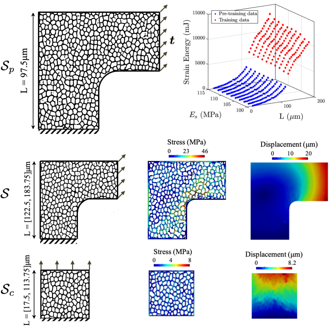
Figure 2: Illustrations of the hierarchy of scenarios and high-fidelity data considered for the surrogate modeling of the elasticity problem: The pre-training scenario $\mathcal{S}_{c}$ consists of smaller domain sizes and under uniaxial loading conditions, while the training scenario $\mathcal{S}$ captures the mechanical features of the target prediction over domain sizes affordable for the high-fidelity model. The prediction scenario $\mathcal{S}_{p}$ involves an aerogel insulation component with a size of $L=297.5\mu m$, and unobservable QoI is the strain energy.

The pre-training dataset $\boldsymbol{D}_{c}$ comprises strain energies computed from 22 equidistant domain sizes within the range of $L=[17.5,113.75]\mu m$, 10 equidistant elastic moduli within $E_{s}=[100,115]$ MPa, and 10 realizations of the aerogel microstructure indicator function $\varphi(\omega,\boldsymbol{y})$. The training set $\boldsymbol{D}$ includes strain energies from high-fidelity simulations obtained at 15 domain sizes within $L=[122.5,183.75]\mu m$, 10 elastic moduli, and 10 microstructure realizations, resulting in a total of 3800 data points in the pre-training and training sets. To assess extrapolation predictions, we consider the leave-out set $\boldsymbol{D}_{LO}$ containing data points with domain sizes $L_{LO}=\{179.4,183.8\}\mu m$. As the validation observables, we take the product of the strain energy and Young’s modulus at a specific domain length $L_{LO}$, evaluated using the high-fidelity simulations and surrogate models, expressed as,

$$\mathcal{Z}_{D}=\int_{E_{s}^{low}}^{E_{s}^{up}}u_{\boldsymbol{D}}|_{L=L_{LO}}\;dE,\quad\quad\mathcal{Z}_{M}=\int_{E_{s}^{low}}^{E_{s}^{up}}u_{\boldsymbol{\theta}}|_{L=L_{LO}}\;dE,$$ (41)

where $E_{s}^{low}=100$ MPa and $E_{s}^{up}=115$ MPa are the range of values for the elastic modulus within the training set. Given the stochastic nature of both observables, we employ two validation measures [84], the normalized Kullback-Leibler divergence by the Shannon entropy,

$$\mathbbm{d}_{DKL}=\frac{\mathcal{D}_{\rm KL}\left(\pi(\mathcal{Z}_{D}),\pi(\mathcal{Z}_{M})\right)}{\mathcal{H}\left(\pi(\mathcal{Z}_{D})\right)},$$ (42)

and discrepancies between cumulative distribution functions,

$$\mathbbm{d}_{CDF}=\int_{-\infty}^{+\infty}|\Phi(\mathcal{Z}_{D})-\Phi(\mathcal{Z}_{M})|d\mathcal{Z}.$$ (43)

5.1.1 Illustrative 1D example

Prior to applying the OPAL-surrogate framework, we conduct a preliminary exploration of the methodologies detailed in Section 3 using a simple 1D example. In this case, the training data $\boldsymbol{D}$ consists of the strain energy calculations with $E_{s}$ = 100 MPa over the domain sizes outlined in the preceding section, exclusion of the pre-training set during inference.

Model plausibility vs. network architecture

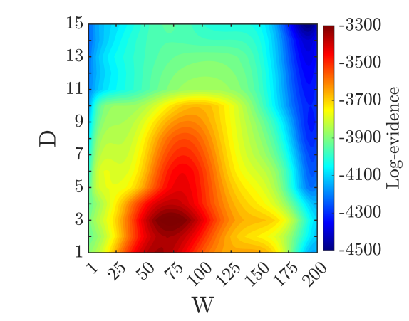
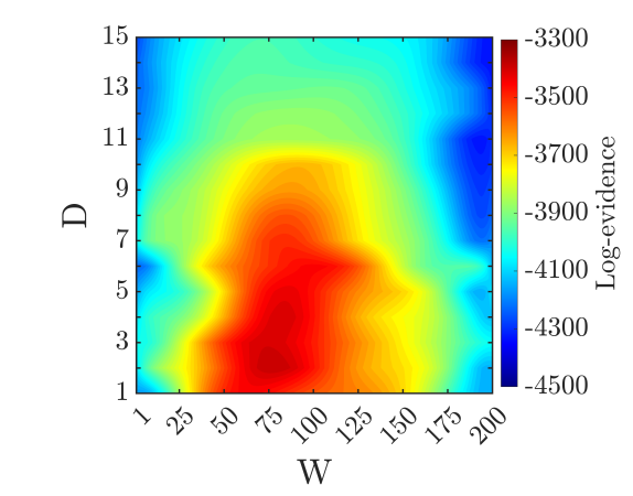
(a)                                                  (b)
 
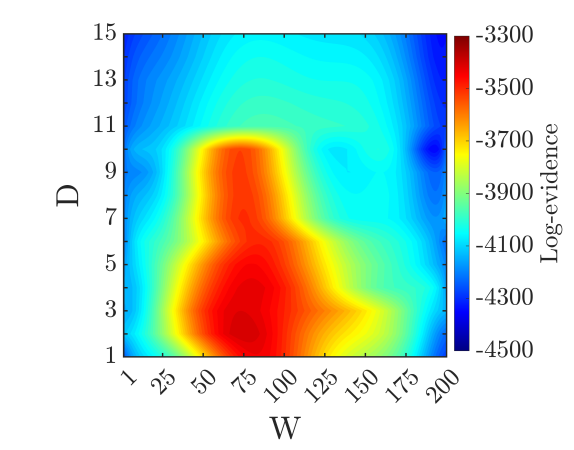
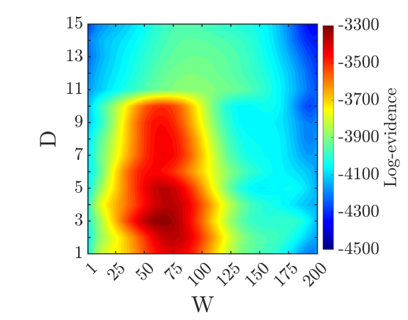
(c)                                                  (d)

Figure 3: Illustrative 1D example: The log-evidence $\ln\pi_{evid}(\boldsymbol{D}|\boldsymbol{\xi}_{i})$, corresponding to posterior model plausibilities $\rho_{i}$ under the uniform prior $\pi_{pr}(\boldsymbol{\xi}_{i})$ assumption, for fully connected BayesNN models with varying number of layers $D$ and neurons in each layer $W$, and activation functions: (a) Tanh, (b) Leaky ReLU, (c) Sigmoid, and (d) ReLU.

Figure 3 illustrates the log-evidence $\ln\pi_{evid}(\boldsymbol{D}|\boldsymbol{\xi}_{i})$ for various fully connected neural networks with different depths $D$ (number of layers), widths $W$ (number of neurons in each layer), and activation functions. Considering uniform prior probabilities $\pi_{pr}(\boldsymbol{\xi}_{i})$ for each model, the log-evidence values are equivalent to the posterior model plausibilities $\rho_{i}$. As depicted in these plots, a specific range of architectural hyperparameters leads to higher plausibilities, implying that the corresponding models have a higher probability of accurately representing the dataset. However, overly simplistic models, characterized by smaller $D$ and $W$, exhibit limited predictive power within the dataset space. Conversely, excessively complex models with larger network parameters can capture a broader range of possible observations with low-confidence predictions within the dataset space. These aspects are clarified in Figure 4, presenting the mean and 95% credible interval (CI) uncertainty in predictions from BayesNN models with Tanh activation functions in comparison to the training data. Models with higher log-evidence (Figure 4(a) and (b)) exhibit more accurate and reliable approximations within and beyond the data range than those with lower log-evidence (Figure 4(c) and (d)).

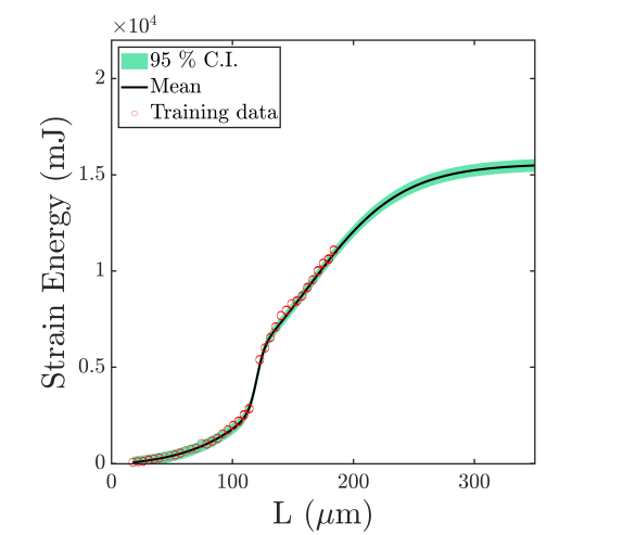
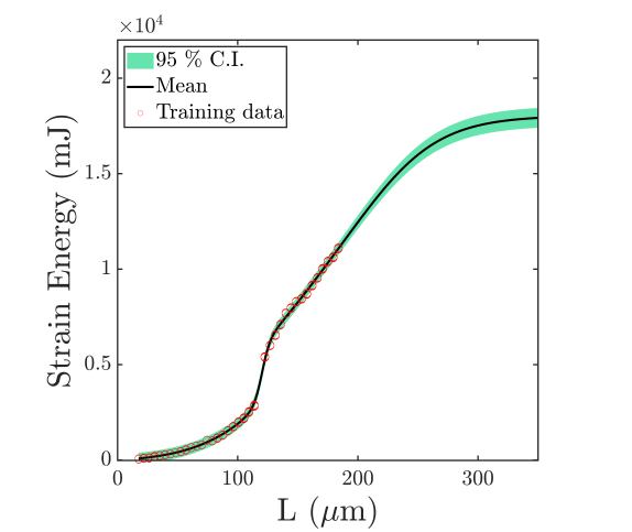
(a)                                                  (b)
 
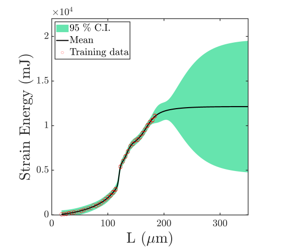
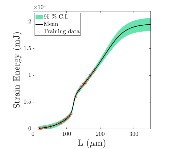
(c)                                                  (d)

Figure 4: Illustrative 1D example: The mean and uncertainty predictions for different fully connected BayesNN models with Tanh activation functions in Figure 3(a) compared to the training data: (a) $D=3$, $W=720$, $\ln\pi_{evid}(\boldsymbol{D}|\boldsymbol{\xi})=-3354$ (highest posterior model plausibility); (b) $D=3$, $W=800$, $\ln\pi_{evid}(\boldsymbol{D}|\boldsymbol{\xi})=-3468$; (c) $D=2$, $W=1450$, $\ln\pi_{evid}(\boldsymbol{D}|\boldsymbol{\xi})=-3877$; (d) $D=1$, $W=1840$, $\ln\pi_{evid}(\boldsymbol{D}|\boldsymbol{\xi})=-3926$.

It’s important to note that model plausibility doesn’t solely represent the prediction credibility, as seen in the faster plateau of the prediction mean in Figure 4(a) compared to (b), and the higher uncertainty bound in Figure 4(c) compared to (d) beyond the training data range. This emphasizes the necessity of validation tests, as discussed in Section 4.1, to rigorously assess surrogate model predictions.

Network sparsification

Figure 5 demonstrates the effectiveness of the sparsification method detailed in Section 4.2 in enhancing model plausibility by eliminating irrelevant network parameters. Gradually increasing $TOL_{\boldsymbol{\theta}}$ initially increases the model evidence, followed by a decline due to excessive sparsification. The reported threshold values correspond to the maximum model evidence. In Figure 5 (a,b), the fully connected network exhibits a plateau in extrapolation with significant uncertainty. Sparsification reduces uncertainty (13.23% in prediction variance) by eliminating irrelevant parameters, albeit with limited enhancement in prediction accuracy. Conversely, Figure 5 (c,d) shows that network sparsification improves accuracy in extrapolation predictions by maintaining the trend in training data for larger values of $L$. While these figures depict two representative cases, additional experiments indicate that the proposed network sparsification generally enhances both accuracy and reliability in BayesNN models.

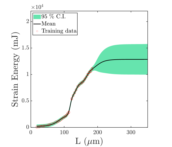
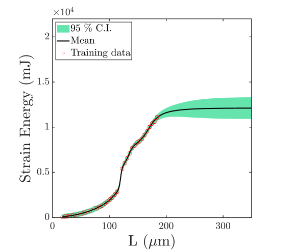
(a)                                                  (b)
 
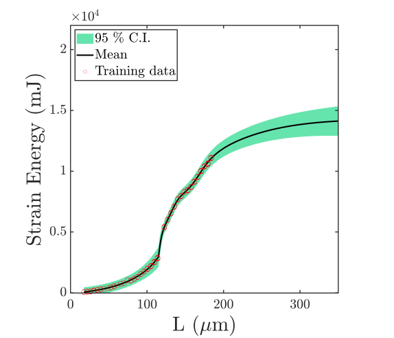
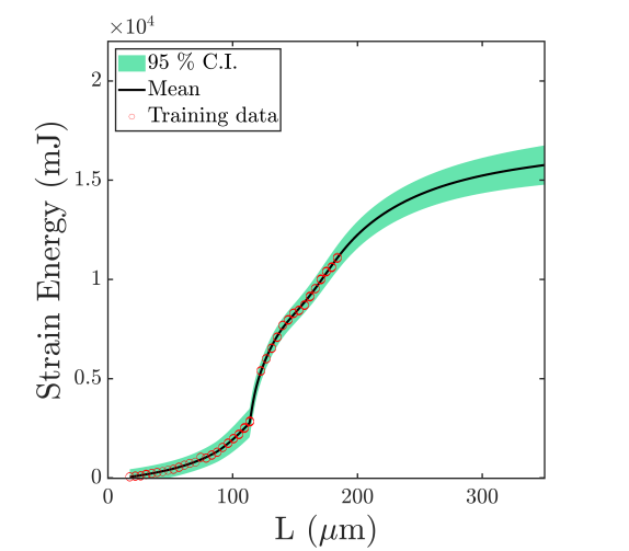
(e)                                                  (f)

Figure 5: Illustrative 1D example: Network sparsification results for the BayesNN models. The mean and uncertainty predictions for (a) the fully connected network with $D=4$, $W=1600$, and $\ln\pi_{evid}(\boldsymbol{D}|\boldsymbol{\xi})=-3821$, and (b) the corresponding sparsified network using $TOL_{\boldsymbol{\theta}}=0.025$, resulting in the elimination of 22% of the parameters and yielding $\ln\pi_{evid}(\boldsymbol{D}|\boldsymbol{\xi})=-3610$. (c) The fully connected network with $D=6$, $W=1700$, and $\ln\pi_{evid}(\boldsymbol{D}|\boldsymbol{\xi})=-3874$, and (d) the corresponding sparsified network using $TOL_{\boldsymbol{\theta}}=0.05$, resulting in the elimination of 32% of the parameters and yielding $\ln\pi_{evid}(\boldsymbol{D}|\boldsymbol{\xi})=-3545$.

5.1.2 OPAL-surrogate demonstration

This section presents the results of identifying the credible surrogate model for predicting the unobservable QoI, the strain energy of the prediction scenario $\mathcal{S}_{p}$, in the elasticity problem, as illustrated in Figure 2. For training the surrogate models and computing the evidence and plausibility, we first infer network parameters using pre-training data $\boldsymbol{D}_{c}$ based on (22) and (23). The resulting posterior serves as the prior for network parameters in hierarchical Bayesian inferences using training data $\boldsymbol{D}$ to evaluate posterior model plausibility.

Determining the initial model set $\mathcal{M}$ and categorization

In defining a sufficiently large model space, we utilize the model evidence (model plausibility) of BayesNNs with a single layer $D=1$, varying widths $W=[1,1200]$, and four activation functions, as depicted in Figure 6. We set the upper limit for width at $W=600$ in the initial model set $\mathcal{M}$, representing a 10% increase over the peak average log-evidences for different functions. Numerical experiments reveal that selecting the upper bound within the range of $W=500$ and $W=800$, minimally impacts the validity and performance of the model identified by OPAL-surrogate. This highlights the effectiveness of the proposed incremental search for initializing OPAL-surrogate with minimal computational overhead. Accordingly, we categorize the BayesNN models with $W=[1,600]$ based on the number of layers, as a measure of model complexity, such that Category 1 encompassing networks with $D=\{1,2\}$, Category 2 including those with $D=\{3,4\}$, and so forth.

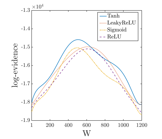
Figure 6: Elasticity problem: The log-evidence (corresponding to model plausibility $\rho$) for BayesNN models with single layer ($D=1$) with different widths and activation functions.

Table 1: Elasticity problem: Identifying the layerwise activation functions based on log-evidence $\pi_{evid}(\boldsymbol{D}|$ $\boldsymbol{\xi}_{(\cdot)}^{l},\boldsymbol{D}_{c},\hat{\mathcal{M}}^{l},\mathcal{S},\mathcal{S}_{c})$. All models are fully connected networks $M^{l}_{F(D,W=600)}$ with depth $D$ and width $W=600$.

Occam	BayesNN	Log-evidence
categories	model	ReLU	Leaky ReLU	Sigmoid	Tanh
$l=1$	$D=1$	-15732	-15045	-15317	-14846
	$D=2$	-15320	-15246	-15314	-14924
$l=2$	$D=3$	-15835	-14834	-15427	-15340
	$D=4$	-15723	-15256	-15417	-15012

Occam Category 1

Tabel 1 shows the values of model evidence $\pi_{evid}$$(\boldsymbol{D}|$ $\boldsymbol{\xi}_{(\cdot)}^{l},\boldsymbol{D}_{c},\hat{\mathcal{M}}^{l},\mathcal{S},\mathcal{S}_{c})$ for fully connected networks $M^{l}_{F(D,W=600)}$ with different activation functions. Accordingly, the Tanh function is selected for the first and second layers. Upon applying sparsification to $M^{1}_{F(D=1,W=600)}$, the plausible model in this category $M^{1}_{I}$ is identified that consists of 564 connections. According to Table 2, the sparsification results in elimination of 6% of the parameters and 0.6% improvement in log-evidence in $M^{1}_{I}$ compared to $M^{1}_{F(D=1,W=600)}$. Figure 7 illustrates the surrogate model predictions of both the fully connected and sparsified networks in comparison to the pre-training and training datasets. The observed increase in model prediction uncertainty at lower $E_{s}$ is attributed to higher uncertainty in high-fidelity simulation data at smaller elastic modulus values captured by the surrogate model.

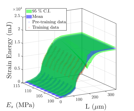
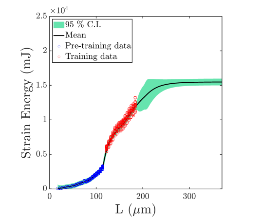
(a)
 
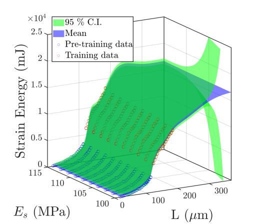
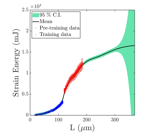
(b)
 
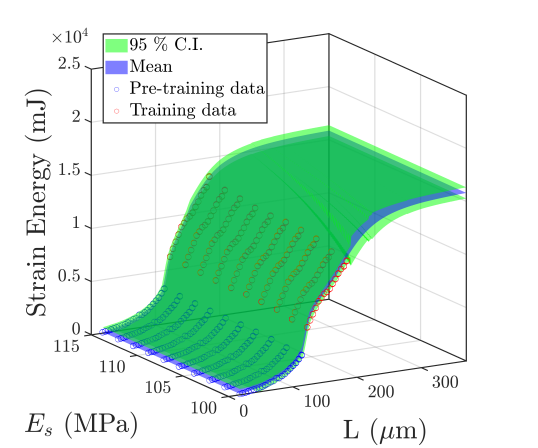
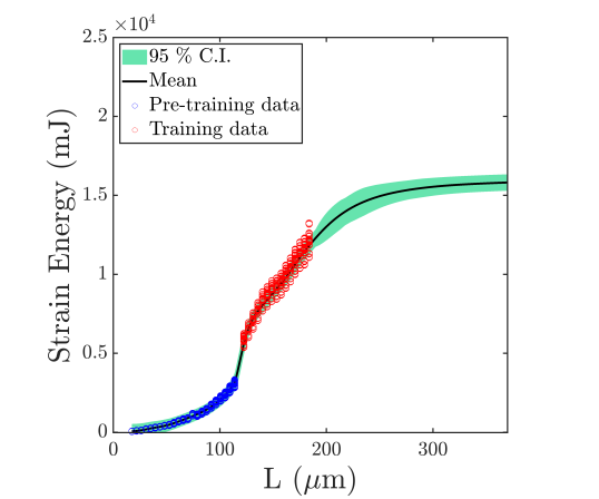
(c)

Figure 7: Elasticity problem: The mean and uncertainty predictions of surrogate models in Category 1 for (a) fully-connected network $M^{1}_{F(D=1,W=600)}$; (b) fully-connected network $M^{1}_{F(D=2,W=600)}$; (c) plausible sparsified network $M^{1}_{I}$ with $D=1$ and 564 connections. The left panels show 3D plots, while the right panels depict the marginalized plots over the $E_{s}$.

Next, we assess the credibility of $M^{1}_{I}$ through a leave-out validation test. The comparison of validation measures for each leave-out data point with the corresponding validation tolerances reveals that $M^{1}_{I}$ fails the validation test and is deemed an invalid model,

$L_{LO}=179.4\mu m$:

$$\mathbbm{d}_{DKL}=0.0112\nleqslant TOL_{DKL}=0.008 \mathbbm{d}_{CDF}=52.31\nleqslant TOL_{CDF}=45,$$ ,

$L_{LO}=183.8\mu m$:

$$\mathbbm{d}_{DKL}=0.0108\nleqslant TOL_{DKL}=0.008 \mathbbm{d}_{CDF}=60.52\nleqslant TOL_{CDF}=45.$$ ,

Occam Category 2

Following the same procedure leads to the selection of the Leaky ReLU activation function for layer 3 and the Tanh function for layer 4. Subsequent sparsification of $M^{2}_{F(D=3,W=600)}$ results in the plausible model within this category, $M^{2}_{I}$, comprising $D=3$ and 619245 connections (approximately 14% parameters reduction upon sparsification). Figure 8 presents the predictions of this surrogate model in comparison to high-fidelity datasets.

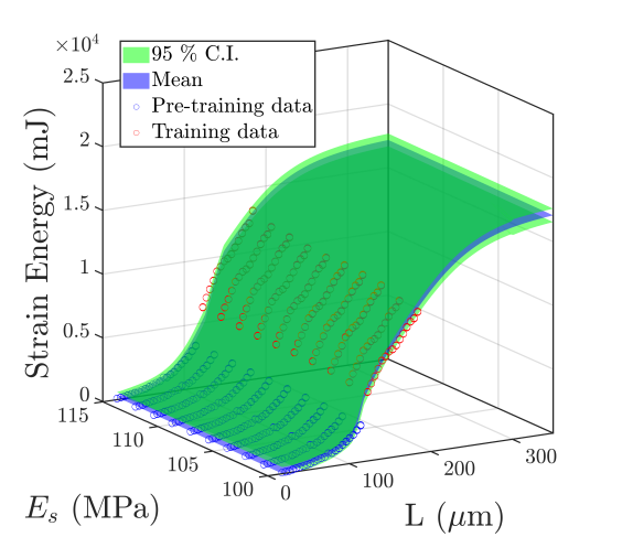
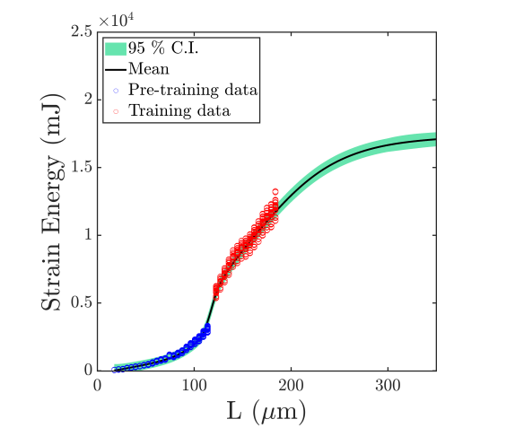
(a)


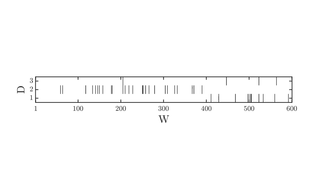
(b)

Figure 8: Elasticity problem: (a) The mean and uncertainty predictions of the plausible sparsified network $M^{2}_{I}$ in Category 2, identified as the “best” surrogate model by OPAL-surrogate.The network consists of 3 layers, 619245 connections, and Tanh, Tanh, Leaky ReLU activation functions for layers 1 to 3, respectively. (b) Visualization of weights pattern for $M^{2}_{F(D=3,W=600)}$ across network depth $D$ and width $W$ in the top panel. The bottom panel illustrates the sparsified pattern of $M^{2}_{I}$, with removed connections marked in black from each hidden layer using $TOL_{\boldsymbol{\theta}}=0.05$.

Importantly, $M^{2}_{I}$ successfully passes the validation test based on both validation metrics,

$L_{LO}=179.4\mu m$:

$$\mathbbm{d}_{DKL}=0.0069\leq TOL_{DKL}=0.008 \mathbbm{d}_{CDF}=40.42\leq TOL_{CDF}=45,$$ ,

$L_{LO}=183.8\mu m$:

$$\mathbbm{d}_{DKL}=0.0061\leq TOL_{DKL}=0.008 \mathbbm{d}_{CDF}=34.55\leq TOL_{CDF}=45,$$ ,

establishing it as the “best” predictive surrogate model for the given pre-training and training data sets. As depicted in Table 2, model $M^{2}_{I}$ demonstrates significantly improved predictive performance compared to $M^{1}_{I}$, as evident from the validation metrics (a 37% reduction in $\mathbbm{d}_{DKL}$ and a 30% decrease in $\mathbbm{d}_{CDF}$), and visually shown in Figure 9.

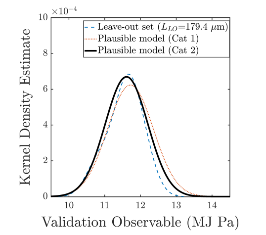
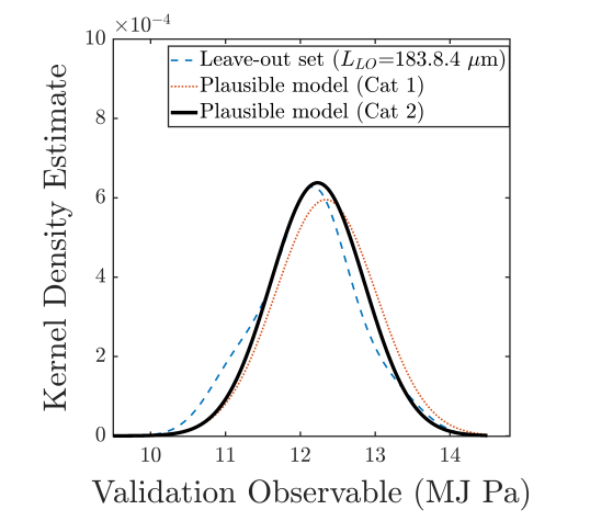
(a)                                                  (b)

Figure 9: Elasticity problem: Comparison of the observables $\mathcal{Z}_{D}$ in (41) corresponding to leave-out validation sets and the predicted $\mathcal{Z}_{M}$ from plausible models $M^{1}_{I}$ and $M^{2}_{I}$ for (a) $L_{LO}=179.4\mu m$; (b) $L_{LO}=183.8\mu m$.

Table 2: Elasticity problem: Results from the implementation of OPAL-surrogate for the identification of the predictive BayesNN surrogate models. $M^{l}_{F(D,W)}$ denotes fully connected networks, and $M^{l}_{I}$ represents the plausible sparsified model in each Occam Category $l$. The values of log-evidence $\pi_{evid}(\boldsymbol{D}|\boldsymbol{\xi}_{(\cdot)}^{l},\boldsymbol{D}_{c},\hat{\mathcal{M}}^{l},\mathcal{S},\mathcal{S}_{c})$ and validation metrics corresponding to leave-out sets $L_{LO}=\{179.4,183.8\}\mu m$ are presented. OPAL-surrogate identifies $M^{2}_{I}$ at Category 2 as the “best” BayesNN surrogate model.

Occam	BayesNN	Activation	$M^{l}_{F(D,W)}$	$M^{l}_{I}$	$\mathbbm{d}_{DKL}$		$\mathbbm{d}_{CDF}$
categories	models	function	log-evid	log-evid	$179.4\mu m$	$183.8\mu m$	$179.4\mu m$	$183.8\mu m$
$l=1$	$D=1$	Tanh	-14846	-14758	0.0112	0.0108	52.31	60.52
	$D=2$	Tanh	-14924
$l=2$	$D=3$	Leaky ReLU	-14834	-14691	0.0073	0.0064	43.62	36.71
	$D=4$	Tanh	-15012
$l=3$	$D=5$	Tanh	-15036	-14882	0.0124	0.0116	85.26	77.42
	$D=6$	Tanh	-15133
$l=4$	$D=7$	LeakyReLU	-15187
	$D=8$	Tanh	-15046	-14962	0.0287	0.0258	153.48	143.21

Exploring higher categories

Although OPAL-surrogate concludes upon identifying the model $M^{2}_{I}$ in Category 2, as depicted in Table 2 and Figure 10, an investigation into the performance of more complex models in higher categories reveals compromised performance. Specifically, models $M^{3}_{I}$ and $M^{4}_{I}$ are deemed invalid based on the specified accuracy tolerance. This highlights the observation that larger networks with increased free parameters do not necessarily translate to improved predictive capabilities.

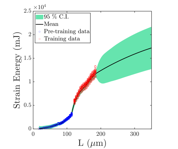
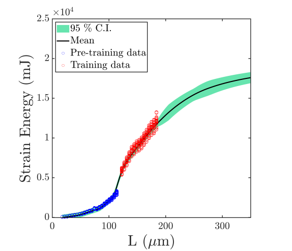
(a)                                                  (b)

Figure 10: Elasticity problem: The mean and uncertainty predictions, marginalized over the $E_{s}$, of surrogate models in Categories 3 and 4: (a) plausible sparsified network $M^{3}_{I}$ with $D=5$ and 1264240 connections; (b) fully-connected network $M^{4}_{F(D=7,W=600)}$. Both panels depict the marginalized plots over the $E_{s}$.

Prediction and forward UQ

Finally, we utilize the surrogate model, $M^{2}_{I}$, to predict and quantify uncertainty in the target QoI (strain energy) in the prediction scenario $\mathcal{S}_{P}$. In Figure 11(a), the surrogate model prediction at $E_{s}=110$ MPa and domain size $L=297.5\mu m$ is compared with one realization of the microstructure in $\mathcal{S}_{P}$, as modeled by high-fidelity simulation. Figure 11(b) presents the probability distributions of the QoI for uncertain elastic modulus of the silica aerogel $E_{s}\sim\mathcal{N}(107.5,112.5)$, as obtained from previous studies [35]. The estimated mean and 95% CI of the QoI for the extrapolation prediction by the BayesNN surrogate model are $\mathbb{E}(QoI)=16615,\quad CI(QoI)=[15565,17665]mJ$. However, considering only the mean of the surrogate model prediction (corresponding to deterministic neural network training), the estimated uncertainty becomes $\mathbb{E}(QoI)=16660,\quad CI(QoI)=[16350,16970]mJ$. These results suggest that while the mean prediction of the surrogate model demonstrates relatively acceptable performance, an evaluation of model prediction uncertainty using BayesNN highlights the intrinsic limitation of neural networks in extrapolation.

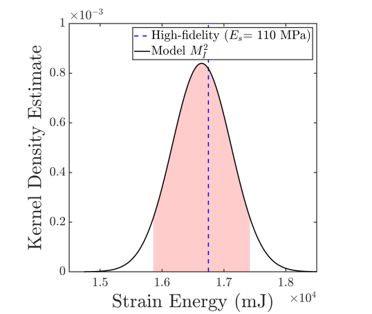
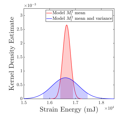
(a)                                                  (b)

Figure 11: Elasticity problem: Prediction of the QoI, strain energy, in the prediction scenario $\mathcal{S}_{P}$, utilizing the BayesNN surrogate model $M^{2}_{I}$, considering: (a) elastic modulus $E_{s}=110$ MPa and in comparison with high-fidelity simulation for one microstructure realization; (b) uncertain elastic modulus $E_{s}\sim\mathcal{N}(107.5,112.5)$ MPa and with and without the inclusion of uncertainty bounds in the model predictions.

5.2 Direct numerical simulations of turbulent combustion

Our second application focuses on the combustion dynamics of shear-induced ablation in solid fuels used in hybrid rocket motors. Specifically, we leverage the Ablative Boundary Layers at the Exascale (ABLATE) software framework [85, 86, 87, 88], which integrates direct numerical simulations of turbulent reacting flows with thermochemical species equations. The focal point of our investigation centers on modeling slab burner experiments according to the setup in [89, 90], designed to study the reacting boundary layer combustion in hybrid rockets and measuring fuel regression rates. Turbulent combustion, occurring over a wide range of time and length scales, involves complex interactions among chemical reactions, flame structures, and the effects of radiation and soot, happening on significantly shorter scales than the flow transport in a combustion chamber. The ABLATE’s Navier-Stokes solver captures these phenomena by simulating the fully compressible and reactive gas phase, including the conservation of mass, momentum, species, and energy balance. The numerical simulations are executed on a grid to ensure adequate representation of turbulence scales, particularly for small Reynolds numbers.

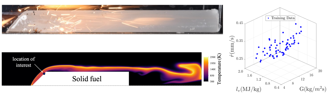
Figure 12: Turbulent combustion problem: The top-left panel illustrates the side profile of the solid fuel in the 2D slab burner experiment [89, 90]. The bottom-left panel displays a representative 2D ABLATE simulation result of the slab burner, highlighting the location on the fuel surface for obtaining fuel regression rate ($\dot{r}$) training data. The right panel shows the training data used for surrogate modeling, comprising an ensemble of $\dot{r}$ for various values of the oxidizer flux ($G$) and latent heat of vaporization ($l_{v}$).

Figure 12 depicts a representative simulation result from a 2D slab burner employed in this study, with Polymethyl methacrylate serving as the solid fuel and $O_{2}$ as the oxidizer in ABLATE simulations. The key output of interest is the fuel regression rate, denoted as $\dot{r}$, representing the rate of fuel recession during combustion and a critical parameter influencing motor thrust and hybrid rocket motor geometry. Given the high computational costs associated with ABLATE simulations, the ultimate aim of the surrogate model is to facilitate Bayesian calibration and validation of ABLATE by utilizing regression rate measurements from slab burner experiments. To this end, we develop a BayesNN surrogate for the fuel regression rate, incorporating two input parameters of ABLATE. The first input is the oxidizer flux $G=[5,20]Kg/m^{2}s$, corresponding to the range of inlet velocities in the slab burner experiment [89, 90], and the second input parameter is the latent heat of vaporization $l_{v}=[6\times 10^{5},11\times 10^{5}]J/Kg$. The training dataset $\boldsymbol{D}$, comprising $N_{D}=64$ simulation ensembles, captures the fuel regression rate $\dot{r}$ at a critical location on the slab boundary (illustrated in Figure 12), with the inputs $G$ and $l_{v}$ sampled using Latin hypercube sampling. For credibility assessment, we consider the leave-out set $\boldsymbol{D}_{LO}$ containing data points within $G_{LO}=[9.89,14.63]Kg/m^{2}s$. The validation observables are,

$$\mathcal{Z}_{D}=\int_{G_{LO}^{low}}^{G_{LO}^{up}}\int_{l_{v}^{low}}^{l_{v}^{up}}u_{\boldsymbol{D}}\;dl_{v}\;dG,\quad\quad\mathcal{Z}_{M}=\int_{G_{LO}^{low}}^{G_{LO}^{up}}\int_{l_{v}^{low}}^{l_{v}^{up}}u_{\boldsymbol{\theta}}\;dl_{v}\;dG,$$ (44)

where $u_{\boldsymbol{D}}$ and $u_{\boldsymbol{\theta}}$ are the fuel regression rate $\dot{r}$, evaluated using the high-fidelity simulations and surrogate models, respectively, and $G_{LO}^{low}=9.89Kg/m^{2}s$, $G_{LO}^{up}=14.63Kg/m^{2}s$, $l_{v}^{low}=6\times 10^{5}J/Kg$, and $l_{v}^{up}=11\times 10^{5}J/Kg$.

OPAL-surrogate demonstration

Following the approach outlined in Section 5.1.2, we set the upper limit for the width at $W=300$ in the initial BayesNN surrogate model set $\mathcal{M}$, guided by Figure 13. Given the smaller dataset, a more strict categorization strategy is employed for models with $W=[1,300]$, with each category corresponding to a distinct width range.

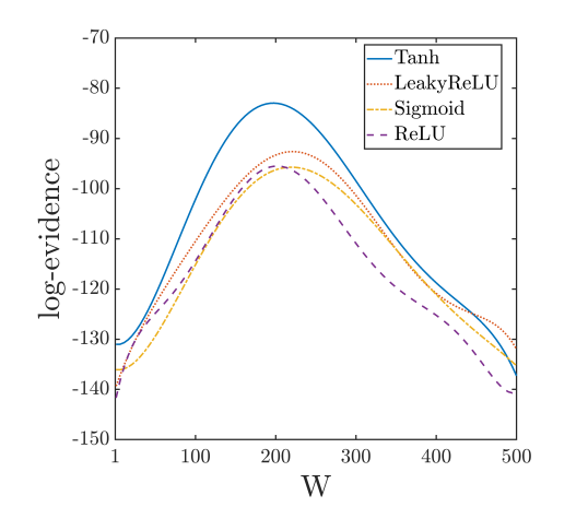
Figure 13: Turbulent combustion problem: The log-evidence for BayesNN models with a single layer ($D=1$) with different widths and activation functions.

Table 3: Turbulent combustion problem: Results from the implementation of OPAL-surrogate for the identification of $M^{2}_{I}$ at Category 2 as the “best” BayesNN surrogate model OPAL-surrogate identifies $M^{2}_{I}$ at Category 2 as the “best” BayesNN surrogate model.

Occam	BayesNN	Activation	$M^{l}_{F(D,W)}$	$M^{l}_{I}$	$\mathbbm{d}_{DKL}$
categories	models	function	log-evid	log-evid
$l=1$	$D=1$	Tanh	-99.5	-95.5	0.0127
$l=2$	$D=2$	Tanh	-94.7	-90.6	0.0084
$l=3$	$D=3$	LeakyReLU	-103.6	-98.7	0.0156

Table 3 presents the results of OPAL-surrogate for the first three categories. Figures 14 and 15(a) illustrate the predictions of both fully connected and sparsified networks in Category 1, comparing them to the training datasets. The plausible model $M^{1}_{I}$ comprises 245 connections, approximately 19% parameter reduction from $M^{1}_{F(D=1,W=300)}$ following sparsification with $TOL_{\boldsymbol{\theta}}=0.075$. However, considering $TOL_{DKL}=0.008$, this model is deemed invalid. Figure 15(a) illustrates the predictions of $M^{1}_{I}$ compared to the leave-out data for credibility assessment.

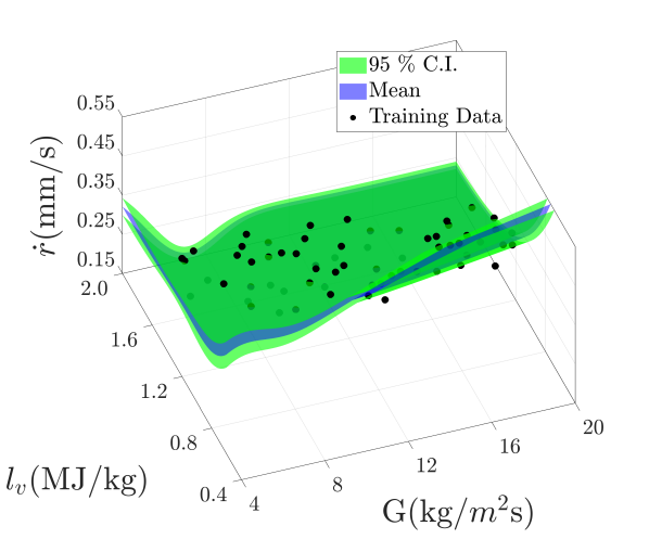
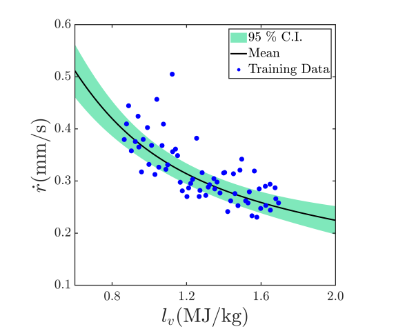
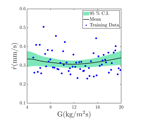
Figure 14: Turbulent combustion problem: The mean and uncertainty predictions of the fully-connected network $M^{1}_{F(D=1,W=300)}$ in Category 1. The top panel shows the 3D plot and the bottom panels display the marginalized plots over the $l_{v}$ and $G$.

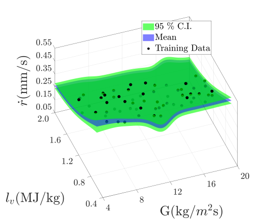
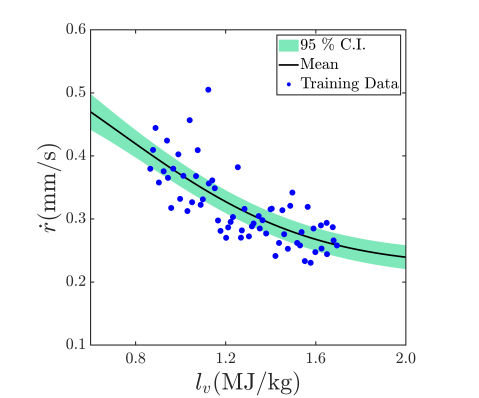
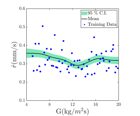
(a)

 
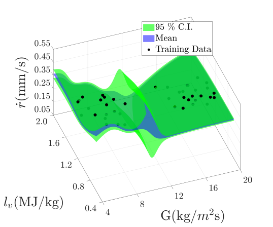
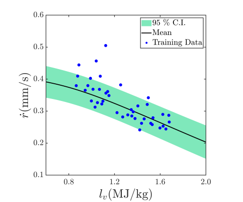
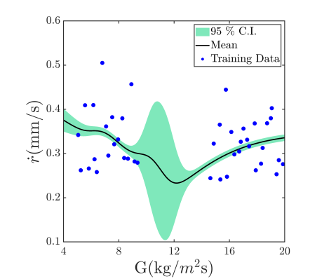
(b)

Figure 15: Turbulent combustion problem: The mean and uncertainty predictions of the plausible sparsified network $M^{1}_{I}$ in Category 1 with $D=1$ and 245 connections in comparison with (a) training data set; (b) leave-out data set. The top panel shows the 3D plot and the bottom panels display the marginalized plots over the $l_{v}$ and $G$.

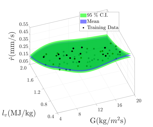
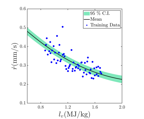
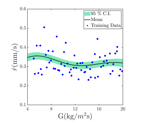
(a)
 
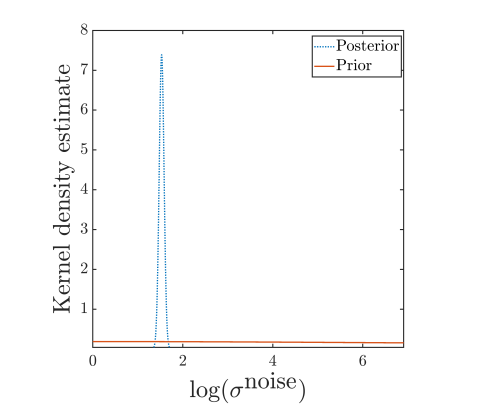
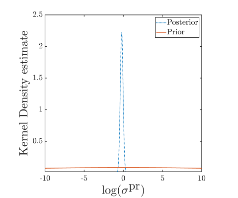
(b)


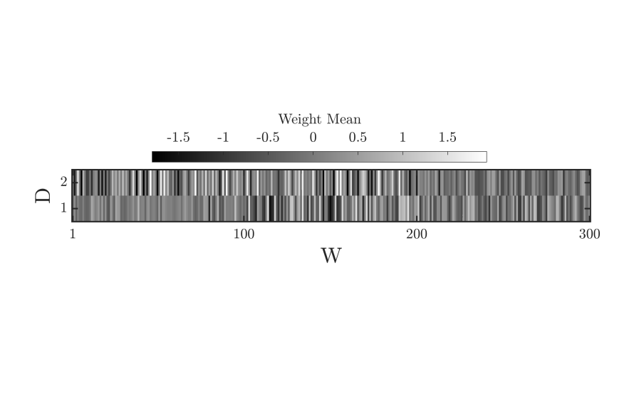
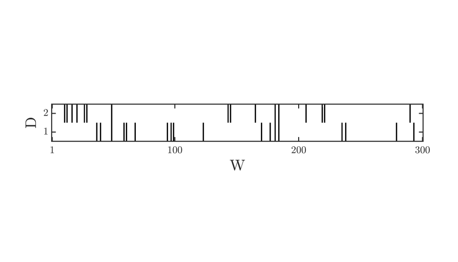
(c)

Figure 16: Turbulent combustion problem: (a) The mean and uncertainty predictions of the plausible sparsified network $M^{2}_{I}$ in Category 2, identified as the “best” surrogate model by OPAL-surrogate. The network consists of 2 layers, 65025 connections, and Tanh activation functions for both layers. (b) Prior and posterior of the inference hyper-parameters. (c) Visualization of weights pattern for $M^{2}_{F(D=2,W=300)}$ across network depth $D$ and width $W$ in the top panel. The bottom panel illustrates the sparsified pattern of $M^{2}_{I}$, with removed connections marked in black from each hidden layer using $TOL_{\boldsymbol{\theta}}=0.12$.

Moving to Category 2, the Tanh activation function is chosen for layer 2. Sparsification of $M^{2}_{F(D=2,W=300)}$ with 90000 connections, results in the plausible model $M^{2}_{I}$ for this category, comprising $D=2$ and 65025 connections, representing approximately 28% reduction in parameters after sparsification with $TOL_{\boldsymbol{\theta}}=0.12$. As shown in Tabel 3, $M^{2}_{I}$ successfully passes the validation test establishing it as the “best” predictive surrogate model. Figure 16 illustrates the predictions of $M^{2}_{I}$ in comparison to the data. The means of the posteriors of the inference hyperparameters shown in this figure are obtained by maximizing the evidence in (3.3), and the posterior variances are approximated using (29). As indicated in Table 3, model $M^{2}_{I}$ demonstrates significantly improved predictive performance compared to $M^{1}_{I}$ and $M^{3}_{I}$ (see Figure 19) in both lower and higher categories. The comparison of validation observables is presented in Figure (18).

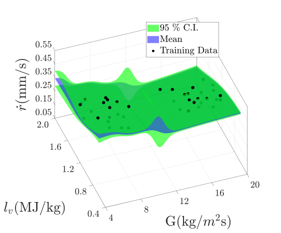
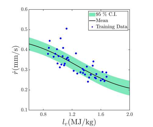
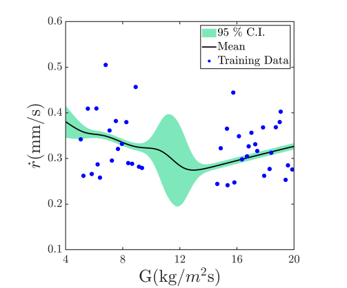
Figure 17: Turbulent combustion problem: The mean and uncertainty predictions of the plausible sparsified network $M^{2}_{I}$ in Category 2 in comparison with the leave-out data. The top panel shows the 3D plot and the bottom panels display the marginalized plots over the $l_{v}$ and $G$.

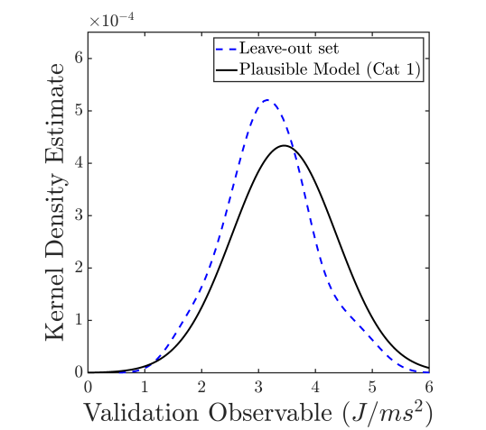
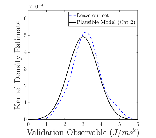
(a)                                                  (b)

Figure 18: Turbulent combustion problem: Comparison of the observables $\mathcal{Z}_{D}$ in (44) corresponding to leave-out validation sets and the predicted $\mathcal{Z}_{M}$ from plausible models $M^{1}_{I}$ and $M^{2}_{I}$.

6 Conclusions

This study introduces OPAL-surrogate, a systematic framework for identifying predictive BayesNN surrogate models within the expansive space of potential models characterized by diverse architectures and hyperparameters. Leveraging hierarchical Bayesian inferences and the concept of model plausibility, OPAL-surrogate efficiently and adaptively adjusts model complexity until satisfying validation criteria. We also stress the significance of well-organized neural network parameters, empowering the surrogate model to effectively capture multiscale interactions encoded in the training data for physics-based simulations. To achieve this, we propose a method involving the sequential addition of fully connected layers with large widths and the elimination of irrelevant weights through an effective network sparsification guided by model evidence.

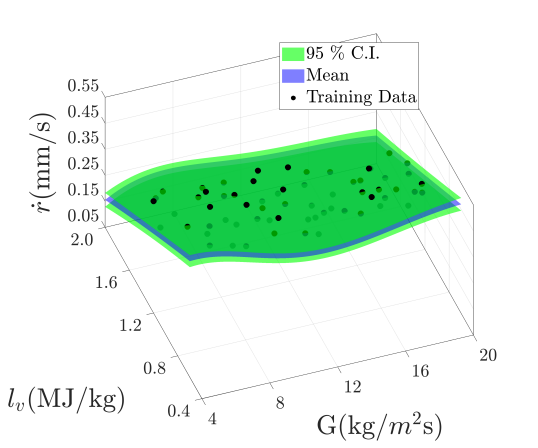
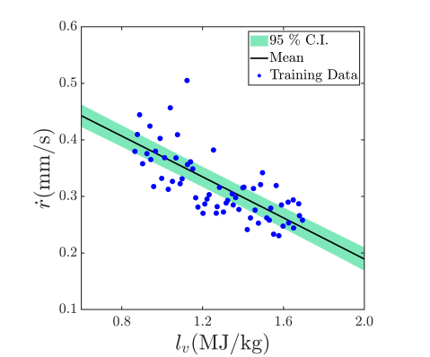
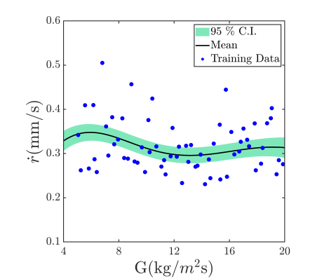
Figure 19: Turbulent combustion problem: The mean and uncertainty predictions of the plausible sparsified network $M^{3}_{I}$ in Category 3 with $D=3$ and 135000 connections in comparison with training data. The top panel shows the 3D plot and the bottom panels display the marginalized plots over the $l_{v}$ and $G$.

Two applications of OPAL-surrogate demonstrate that the identified architecture and hyperparameters of the BayesNN model, achieved through a balanced trade-off between model complexity and validity, result in enhanced accuracy and reliability in predictions. The first example involves surrogate modeling of elastic deformation in porous materials, aiming to facilitate quantifying uncertainty in unobservable QoI for domain sizes where high-fidelity simulation is computationally prohibitive. The results suggest that, despite a substantial training dataset comprising 1500 data points and constructing the prior for network parameters from the pre-training dataset, the extrapolation prediction capability of the identified BayesNN model remains credible only up to 1.5 times the size of the training domain. Beyond this point, the accuracy and reliability of the prediction rapidly decline, highlighting the necessity of imposing physical constraints to enhance the extrapolation abilities of neural networks, e.g., [91, 92, 93]. The second numerical experiment involves a turbulent combustion flow model of a slab burner, where OPAL-surrogate successfully identifies the BayesNN surrogate model for the fuel regression rate based on 64 training data points.

We highlight a fundamental misconception contributing to overconfident predictions – the notion that the complexity of a predictive model must always be limited when training data is scarce. In contrast, the OPAL-surrogate framework relies on Bayesian inference without the constraint of modifying the model and prior based on the data volume. In fact, we argue that there is never enough high-fidelity data from physical simulations for surrogate model construction. Thus, OPAL-surrogate embodies an open-ended inference approach, continuously refining the predictive surrogate model, as that additional data and information could potentially falsify a model initially presumed to be valid. In constructing the initial set of possible models, [24, 94, 95] propose incorporating models we genuinely believe in, along with every conceivable sub-model, ensuring that the model selection strategy can identify the sub-model that best explains the data.

In advancing the surrogate modeling using the proposed framework in this work, several avenues can be explored in future studies. Firstly, more accurate Bayesian solutions may be adopted, recognizing that the posterior distribution is only asymptotically normally distributed as the number of data points approaches infinity, and in neural networks, they might be multi-modal. Despite this, given the Laplace approximation’s high efficiency and scalability compared to other existing algorithms, it may be worthwhile to expand the definition of the BayesNN model, incorporating various solutions with differing complexities into the initial model set. Subsequently, OPAL-surrogate can discern the one that provides valid predictions. This approach is justified by the primary goal of the surrogate model, which is to faithfully approximate the predictive distribution rather than the accuracy of parameter inference. Secondly, there is a need for comprehensive investigations into effective methods for revealing neural network sparsity patterns associated with multiscale physical phenomena. This can involve exploring techniques like probabilistic sparse masks, e.g., [96, 78] and leveraging architecture search algorithms, e.g., [32], with the potential to enhance sparsification efficiency after replacing the performance measure with model evidence. Thirdly, expanding upon [74, 21], a goal-oriented design of training scenarios within Step 5 of OPAL-surrogate could be investigated. This involves employing active subspace methods to generate high-fidelity data that accurately reflects the structure of the prediction QoI. Fourthly, addressing the unresolved challenge of surrogate model-form uncertainty is imperative for achieving improved accuracy and reliability in extrapolation. One potential path involves exploiting the underlying structure of high-fidelity solutions through a-posteriori error estimation and its associated computable uncertainty bounds, e.g., [97, 98, 99, 92, 100, 101]. Lastly, in the future, we aim to enhance the versatility of OPAL-surrogate to accommodate a broader range of possible models, e.g., different classes of neural operators [102, 103, 104, 105, 106, 107, 108, 109]. This expansion could significantly reinforce its capacity to identify the appropriate surrogate model for a given problem.

In conclusion, this study highlights the substantial challenges associated with the discovery and assessing the credibility of neural network-based surrogate models for complex multiscale and multiphysics simulations. The introduced framework aims to tackle some of these challenges by highlighting the crucial interplay between model complexity and rigorous validation. It provides a foundation for future research to enhance its efficacy and extend its applicability across diverse classes of surrogate models.

References

-
[1]
R. K. Tripathy, I. Bilionis, Deep UQ: Learning deep neural network surrogate models for high dimensional uncertainty quantification, Journal of Computational Physics 375 (2018) 565–588.
doi:https://doi.org/10.1016/j.jcp.2018.08.036.
URL https://www.sciencedirect.com/science/article/pii/S0021999118305655 -
[2]
Y. Zhu, N. Zabaras, Bayesian deep convolutional encoder–decoder networks for surrogate modeling and uncertainty quantification, Journal of Computational Physics 366 (2018) 415–447.
doi:https://doi.org/10.1016/j.jcp.2018.04.018.
URL https://www.sciencedirect.com/science/article/pii/S0021999118302341 - [3] G. Georgalis, K. Retfalvi, P. E. Desjardin, A. Patra, Combined data and deep learning model uncertainties: An application to the measurement of solid fuel regression rate, International Journal for Uncertainty Quantification 13 (5) (1 2023). doi:10.1615/int.j.uncertaintyquantification.2023046610.
- [4] Y. Li, Y. Wang, L. Yan, Surrogate modeling for bayesian inverse problems based on physics-informed neural networks, Journal of Computational Physics 475 (2023) 111841.
- [5] L. Cao, K. Wu, J. T. Oden, P. Chen, O. Ghattas, Bayesian model calibration for diblock copolymer thin film self-assembly using power spectrum of microscopy data and machine learning surrogate, Computer Methods in Applied Mechanics and Engineering 417 (2023) 116349.
- [6] D. Luo, T. O’Leary-Roseberry, P. Chen, O. Ghattas, Efficient pde-constrained optimization under high-dimensional uncertainty using derivative-informed neural operators, arXiv preprint arXiv:2305.20053 (2023).
- [7] A. Chattopadhyay, M. Gray, T. Wu, A. B. Lowe, R. He, Oceannet: A principled neural operator-based digital twin for regional oceans, arXiv preprint arXiv:2310.00813 (2023).
- [8] Q. He, M. Perego, A. A. Howard, G. E. Karniadakis, P. Stinis, A hybrid deep neural operator/finite element method for ice-sheet modeling, arXiv preprint arXiv:2301.11402 (2023).
- [9] M. G. Kapteyn, J. V. Pretorius, K. E. Willcox, A probabilistic graphical model foundation for enabling predictive digital twins at scale, Nature Computational Science 1 (5) (2021) 337–347.
- [10] S. Mowlavi, S. Nabi, Optimal control of pdes using physics-informed neural networks, Journal of Computational Physics 473 (2023) 111731.
- [11] T. Zohdi, A digital-twin and machine-learning framework for precise heat and energy management of data-centers, Computational Mechanics 69 (6) (2022) 1501–1516.
- [12] K. Wu, T. O’Leary-Roseberry, P. Chen, O. Ghattas, Large-scale Bayesian optimal experimental design with derivative-informed projected neural network, Journal of Scientific Computing 95 (1) (2023) 30.
- [13] J. Stuckner, M. Piekenbrock, S. M. Arnold, T. M. Ricks, Optimal experimental design with fast neural network surrogate models, Computational Materials Science 200 (2021) 110747.
- [14] A. Arzani, L. Yuan, P. Newell, B. Wang, Interpreting and generalizing deep learning in physics-based problems with functional linear models, arXiv preprint arXiv:2307.04569 (2023).
- [15] L. Yuan, H. S. Park, E. Lejeune, Towards out of distribution generalization for problems in mechanics, Computer Methods in Applied Mechanics and Engineering 400 (2022) 115569.
- [16] W. Samek, G. Montavon, S. Lapuschkin, C. J. Anders, K.-R. Müller, Explaining deep neural networks and beyond: A review of methods and applications, Proceedings of the IEEE 109 (3) (2021) 247–278.
- [17] X. Zhong, B. Gallagher, S. Liu, B. Kailkhura, A. Hiszpanski, T. Y.-J. Han, Explainable machine learning in materials science, npj Computational Materials 8 (1) (2022) 204.
- [18] T. Oden, R. Moser, O. Ghattas, Computer Predictions with Quantified Uncertainty, Part I, SIAM News 43 (9) (2010).
-
[19]
I. Babuška, F. Nobile, R. Tempone, A systematic approach to model validation based on Bayesian updates and prediction related rejection criteria, Computer Methods in Applied Mechanics and Engineering 197 (29) (2008) 2517–2539, validation Challenge Workshop.
doi:https://doi.org/10.1016/j.cma.2007.08.031.
URL https://www.sciencedirect.com/science/article/pii/S0045782507005142 - [20] J. T. Oden, I. Babuška, D. Faghihi, Predictive computational science: Computer predictions in the presence of uncertainty, Encyclopedia of Computational Mechanics Second Edition (2017) 1–26.
- [21] J. Tan, B. Liang, P. K. Singh, K. A. Farrell-Maupin, D. Faghihi, Toward selecting optimal predictive multiscale models, Computer Methods in Applied Mechanics and Engineering 402 (2022) 115517.
- [22] M. Yaseen, X. Wu, Quantification of deep neural network prediction uncertainties for vvuq of machine learning models, Nuclear Science and Engineering 197 (5) (2023) 947–966.
- [23] J. M. Twomey, A. E. Smith, et al., Validation and verification, Artificial neural networks for civil engineers: Fundamentals and applications (1997) 44–64.
- [24] D. J. MacKay, Probable networks and plausible predictions-a review of practical Bayesian methods for supervised neural networks, Network: computation in neural systems 6 (3) (1995) 469.
- [25] R. M. Neal, Bayesian learning for neural networks, Vol. 118, Springer Science & Business Media, 2012.
- [26] T. Elsken, J. H. Metzen, F. Hutter, Neural architecture search: A survey, The Journal of Machine Learning Research 20 (1) (2019) 1997–2017.
- [27] Y. Liu, Y. Sun, B. Xue, M. Zhang, G. G. Yen, K. C. Tan, A survey on evolutionary neural architecture search, IEEE transactions on neural networks and learning systems (2021).
- [28] B. Wang, Y. Sun, B. Xue, M. Zhang, A hybrid differential evolution approach to designing deep convolutional neural networks for image classification, in: AI 2018: Advances in Artificial Intelligence: 31st Australasian Joint Conference, Wellington, New Zealand, December 11-14, 2018, Proceedings 31, Springer, 2018, pp. 237–250.
- [29] A. Ghosh, N. D. Jana, S. Mallik, Z. Zhao, Designing optimal convolutional neural network architecture using differential evolution algorithm, Patterns 3 (9) (2022) 100567.
- [30] H. Mendoza, A. Klein, M. Feurer, J. T. Springenberg, F. Hutter, Towards automatically-tuned neural networks, in: Workshop on automatic machine learning, PMLR, 2016, pp. 58–65.
- [31] F. Hutter, L. Kotthoff, J. Vanschoren (Eds.), Automated Machine Learning - Methods, Systems, Challenges, Springer, 2019.
- [32] T. Akiba, S. Sano, T. Yanase, T. Ohta, M. Koyama, Optuna: A next-generation hyperparameter optimization framework, in: Proceedings of the 25th ACM SIGKDD International Conference on Knowledge Discovery and Data Mining, 2019.
- [33] D. Faghihi, S. Sarkar, M. Naderi, J. E. Rankin, L. Hackel, N. Iyyer, A probabilistic design method for fatigue life of metallic component, ASCE-ASME Journal of Risk and Uncertainty in Engineering Systems, Part B: Mechanical Engineering 4 (3) (2018).
- [34] J. Tan, U. Villa, N. Shamsaei, S. Shao, H. M. Zbib, D. Faghihi, A predictive discrete-continuum multiscale model of plasticity with quantified uncertainty, International Journal of Plasticity 138 (2021) 102935.
- [35] J. Tan, P. Maleki, L. An, M. Di Luigi, U. Villa, C. Zhou, S. Ren, D. Faghihi, A predictive multiphase model of silica aerogels for building envelope insulations, Computational Mechanics 69 (6) (2022) 1457–1479.
- [36] J. T. Oden, E. E. Prudencio, A. Hawkins-Daarud, Selection and assessment of phenomenological models of tumor growth, Mathematical Models and Methods in Applied Sciences 23 (07) (2013) 1309–1338.
- [37] P. K. Jha, L. Cao, J. T. Oden, Bayesian-based predictions of covid-19 evolution in texas using multispecies mixture-theoretic continuum models, Computational Mechanics 66 (5) (2020) 1055–1068.
- [38] B. Liang, J. Tan, L. Lozenski, D. A. Hormuth II, T. E. Yankeelov, U. Villa, D. Faghihi, Bayesian inference of tissue heterogeneity for individualized prediction of glioma growth, IEEE Transactions on Medical Imaging (2023).
- [39] E. A. Lima, D. Faghihi, R. Philley, J. Yang, J. Virostko, C. M. Phillips, T. E. Yankeelov, Bayesian calibration of a stochastic, multiscale agent-based model for predicting in vitro tumor growth, PLoS Computational Biology 17 (11) (2021) e1008845.
- [40] E. Prudencio, P. Bauman, D. Faghihi, K. Ravi-Chandar, J. Oden, A computational framework for dynamic data-driven material damage control, based on Bayesian inference and model selection, International Journal for Numerical Methods in Engineering 102 (3-4) (2015) 379–403.
- [41] K. Farrell, J. T. Oden, D. Faghihi, A Bayesian framework for adaptive selection, calibration, and validation of coarse-grained models of atomistic systems, Journal of Computational Physics 295 (2015) 189–208.
- [42] J. T. Oden, E. A. Lima, R. C. Almeida, Y. Feng, M. N. Rylander, D. Fuentes, D. Faghihi, M. M. Rahman, M. DeWitt, M. Gadde, et al., Toward predictive multiscale modeling of vascular tumor growth, Archives of Computational Methods in Engineering 23 (4) (2016) 735–779.
- [43] D. J. MacKay, Bayesian interpolation, Neural computation 4 (3) (1992) 415–447.
- [44] C. M. Bishop, Bayesian methods for neural networks (1995).
- [45] A. F. Psaros, X. Meng, Z. Zou, L. Guo, G. E. Karniadakis, Uncertainty quantification in scientific machine learning: Methods, metrics, and comparisons, Journal of Computational Physics (2023) 111902.
-
[46]
L. Yang, X. Meng, G. E. Karniadakis, B-pinns: Bayesian physics-informed neural networks for forward and inverse pde problems with noisy data, Journal of Computational Physics 425 (2021) 109913.
doi:https://doi.org/10.1016/j.jcp.2020.109913.
URL https://www.sciencedirect.com/science/article/pii/S0021999120306872 - [47] A. Olivier, M. D. Shields, L. Graham-Brady, Bayesian neural networks for uncertainty quantification in data-driven materials modeling, Computer methods in applied mechanics and engineering 386 (2021) 114079.
-
[48]
K. Linka, A. Schäfer, X. Meng, Z. Zou, G. E. Karniadakis, E. Kuhl, Bayesian physics informed neural networks for real-world nonlinear dynamical systems, Computer Methods in Applied Mechanics and Engineering 402 (2022) 115346, a Special Issue in Honor of the Lifetime Achievements of J. Tinsley Oden.
doi:https://doi.org/10.1016/j.cma.2022.115346.
URL https://www.sciencedirect.com/science/article/pii/S0045782522004327 -
[49]
C. Mora, J. T. Eweis-Labolle, T. Johnson, L. Gadde, R. Bostanabad, Probabilistic neural data fusion for learning from an arbitrary number of multi-fidelity data sets, Computer Methods in Applied Mechanics and Engineering 415 (2023) 116207.
doi:https://doi.org/10.1016/j.cma.2023.116207.
URL https://www.sciencedirect.com/science/article/pii/S0045782523003316 - [50] K. Kontolati, S. Goswami, M. D. Shields, G. E. Karniadakis, On the influence of over-parameterization in manifold based surrogates and deep neural operators, Journal of Computational Physics 479 (2023) 112008.
- [51] X. Meng, H. Babaee, G. E. Karniadakis, Multi-fidelity Bayesian neural networks: Algorithms and applications, Journal of Computational Physics 438 (2021) 110361.
- [52] P. Thiagarajan, P. Khairnar, S. Ghosh, Explanation and use of uncertainty quantified by Bayesian neural network classifiers for breast histopathology images, IEEE Transactions on medical imaging 41 (4) (2021) 815–825.
- [53] R. M. Neal, Bayesian training of backpropagation networks by the hybrid monte carlo method, Tech. rep., Citeseer (1992).
- [54] C. M. Bishop, Neural networks for pattern recognition, Oxford university press, 1995.
- [55] W. Buntine, A. Weigend, Bayesian back-propagation. technical report fia-91-22 (1991).
- [56] H. Ritter, A. Botev, D. Barber, A scalable laplace approximation for neural networks, in: 6th International Conference on Learning Representations, ICLR 2018-Conference Track Proceedings, Vol. 6, International Conference on Representation Learning, 2018.
- [57] M. Humt, Laplace approximation for uncertainty estimation of deep neural networks, Ph.D. thesis, TUM (2019).
- [58] A. Immer, M. Bauer, V. Fortuin, G. Rätsch, K. M. Emtiyaz, Scalable marginal likelihood estimation for model selection in deep learning, in: International Conference on Machine Learning, PMLR, 2021, pp. 4563–4573.
- [59] J. Martens, R. Grosse, Optimizing neural networks with kronecker-factored approximate curvature, in: International conference on machine learning, PMLR, 2015, pp. 2408–2417.
- [60] A. Botev, H. Ritter, D. Barber, Practical gauss-newton optimisation for deep learning, in: International Conference on Machine Learning, PMLR, 2017, pp. 557–565.
- [61] Z. Deng, F. Zhou, J. Zhu, Accelerated linearized laplace approximation for bayesian deep learning, Advances in Neural Information Processing Systems 35 (2022) 2695–2708.
- [62] A. Immer, M. Korzepa, M. Bauer, Improving predictions of bayesian neural nets via local linearization, in: International conference on artificial intelligence and statistics, PMLR, 2021, pp. 703–711.
- [63] K. Qian, A. S. Liao, S. Gu, V. A. Webster-Wood, Y. J. Zhang, Biomimetic iga neuron growth modeling with neurite morphometric features and cnn-based prediction, Computer Methods in Applied Mechanics and Engineering 417 (2023) 116213.
- [64] Y. Yao, A. Vehtari, D. Simpson, A. Gelman, Using stacking to average Bayesian predictive distributions (with discussion) (2018).
- [65] M. Muto, J. L. Beck, Bayesian updating and model class selection for hysteretic structural models using stochastic simulation, Journal of Vibration and Control 14 (1-2) (2008) 7–34.
- [66] C. K. Williams, C. E. Rasmussen, Gaussian processes for machine learning, Vol. 2, MIT press Cambridge, MA, 2006.
- [67] J.-P. Vila, V. Wagner, P. Neveu, Bayesian nonlinear model selection and neural networks: A conjugate prior approach, IEEE Transactions on neural networks 11 (2) (2000) 265–278.
- [68] N. Chitsazan, A. A. Nadiri, F. T.-C. Tsai, Prediction and structural uncertainty analyses of artificial neural networks using hierarchical bayesian model averaging, Journal of Hydrology 528 (2015) 52–62.
- [69] P. Shekhar, A. Patra, A forward–backward greedy approach for sparse multiscale learning, Computer Methods in Applied Mechanics and Engineering 400 (2022) 115420.
- [70] P. Shekhar, A. Patra, Hierarchical approximations for data reduction and learning at multiple scales, Foundations of Data Science 2 (2) (2020) 123–154.
- [71] X. Huan, Y. M. Marzouk, Simulation-based optimal Bayesian experimental design for nonlinear systems, Journal of Computational Physics 232 (1) (2013) 288–317.
- [72] C. Riis, F. Antunes, F. Hüttel, C. Lima Azevedo, F. Pereira, Bayesian active learning with fully bayesian gaussian processes, Advances in Neural Information Processing Systems 35 (2022) 12141–12153.
- [73] R. Dehghannasiri, B.-J. Yoon, E. R. Dougherty, Efficient experimental design for uncertainty reduction in gene regulatory networks, in: BMC bioinformatics, Vol. 16, BioMed Central, 2015, pp. 1–18.
- [74] A. Paquette-Rufiange, S. Prudhomme, M. Laforest, Optimal design of validation experiments for the prediction of quantities of interest, arXiv preprint arXiv:2303.06114 (2023).
- [75] S. H. Rudy, T. P. Sapsis, Sparse methods for automatic relevance determination, Physica D: Nonlinear Phenomena 418 (2021) 132843.
- [76] S. Zhang, G. Lin, Robust data-driven discovery of governing physical laws with error bars, Proceedings of the Royal Society A: Mathematical, Physical and Engineering Sciences 474 (2217) (2018) 20180305.
- [77] R. Fuentes, N. Dervilis, K. Worden, E. J. Cross, Efficient parameter identification and model selection in nonlinear dynamical systems via sparse bayesian learning, in: Journal of Physics: Conference Series, Vol. 1264, IOP Publishing, 2019, p. 012050.
- [78] P. M. Williams, Bayesian regularization and pruning using a laplace prior, Neural computation 7 (1) (1995) 117–143.
- [79] E. T. Jaynes, Probability theory: The logic of science, Cambridge University press, 2003.
- [80] E. T. Jaynes, Prior probabilities, IEEE Transactions on systems science and cybernetics 4 (3) (1968) 227–241.
- [81] A. Sarkar, P. K. Singh, L. Zhu, D. Faghihi, S. Ren, Carbon-sequestration straw cellulose-aerogel gradient thermal insulation material, ACS Applied Engineering Materials (2024).
- [82] L. An, M. Di Luigi, J. Tan, D. Faghihi, S. Ren, Flexible percolation fibrous thermal insulating composite membranes for thermal management, Materials Advances 4 (1) (2023) 284–290.
- [83] S. Bhattacharjee, Integrating scientific machine learning and physics-based models for quantification of uncertainty in thermal properties of silica aerogel, Ph.D. thesis, State University of New York at Buffalo (2023).
- [84] K. A. Maupin, L. P. Swiler, N. W. Porter, Validation metrics for deterministic and probabilistic data, Journal of Verification, Validation and Uncertainty Quantification 3 (3) (2018) 031002.
- [85] K. Budzinski, S. S. Aphale, E. K. Ismael, G. Surina III, P. E. DesJardin, Radiation heat transfer in ablating boundary layer combustion theory used for hybrid rocket motor analysis, Combustion and Flame 217 (2020) 248–261.
- [86] K. Retfalvi, E. K. Ismael, K. L. Budzinski, M. McGurn, P. DesJardin, Direct numerical simulation and measurements of a solid fuel slab burner experiment, in: AIAA SCITECH 2024 Forum, 2024, p. 1183.
- [87] R. Zangeneh, P. DesJardin, J. M. Chen, Scaling boundary-layer profile of turbulent wall flows with mass transfer, in: AIAA SCITECH 2024 Forum, 2024, p. 2196.
- [88] M. McGurn, D. Salac, Ablate ablative boundary layers at the exascale, version 0.12.23, https://ablate.dev (2013).
- [89] G. Georgalis, K. Retfalvi, P. E. DesJardin, A. Patra, Combined data and deep learning model uncertainties: An application to the measurement of solid fuel regression rate, International Journal for Uncertainty Quantification 13 (5) (2023).
- [90] G. Surina III, G. Georgalis, S. S. Aphale, A. Patra, P. E. DesJardin, Measurement of hybrid rocket solid fuel regression rate for a slab burner using deep learning, Acta Astronautica 190 (2022) 160–175.
- [91] M. Raissi, P. Perdikaris, G. E. Karniadakis, Physics-informed neural networks: A deep learning framework for solving forward and inverse problems involving nonlinear partial differential equations, Journal of Computational physics 378 (2019) 686–707.
-
[92]
P. K. Jha, J. T. Oden, Residual-based error corrector operator to enhance accuracy and reliability of neural operator surrogates of nonlinear variational boundary-value problems, Computer Methods in Applied Mechanics and Engineering 419 (2024) 116595.
doi:https://doi.org/10.1016/j.cma.2023.116595.
URL https://www.sciencedirect.com/science/article/pii/S0045782523007193 - [93] A. Li, Y. J. Zhang, Isogeometric analysis-based physics-informed graph neural network for studying traffic jam in neurons, Computer Methods in Applied Mechanics and Engineering 403 (2023) 115757.
- [94] G. E. Box, Robustness in the strategy of scientific model building, Robustness in statistics 1 (1979) 201–236.
- [95] G. E. Box, G. C. Tiao, Bayesian inference in statistical analysis, John Wiley & Sons, 2011.
- [96] X. Zhou, W. Zhang, H. Xu, T. Zhang, Effective sparsification of neural networks with global sparsity constraint, in: Proceedings of the IEEE/CVF Conference on Computer Vision and Pattern Recognition, 2021, pp. 3599–3608.
- [97] J. T. Oden, S. Prudhomme, Estimation of modeling error in computational mechanics, Journal of Computational Physics 182 (2) (2002) 496–515.
- [98] K. S. Vemaganti, J. T. Oden, Estimation of local modeling error and goal-oriented adaptive modeling of heterogeneous materials: Part ii: a computational environment for adaptive modeling of heterogeneous elastic solids, Computer Methods in Applied Mechanics and Engineering 190 (46-47) (2001) 6089–6124.
- [99] J. T. Oden, K. Farrell, D. Faghihi, Estimation of error in observables of coarse-grained models of atomic systems, Advanced Modeling and Simulation in Engineering Sciences 2 (1) (2015) 1–20.
- [100] L. Cao, T. O’Leary-Roseberry, P. K. Jha, J. T. Oden, O. Ghattas, Residual-based error correction for neural operator accelerated infinite-dimensional bayesian inverse problems, Journal of Computational Physics 486 (2023) 112104.
- [101] P. K. Jha, J. T. Oden, Goal-oriented a-posteriori estimation of model error as an aid to parameter estimation, Journal of Computational Physics 470 (2022) 111575.
- [102] T. O’Leary-Roseberry, X. Du, A. Chaudhuri, J. R. Martins, K. Willcox, O. Ghattas, Learning high-dimensional parametric maps via reduced basis adaptive residual networks, Computer Methods in Applied Mechanics and Engineering 402 (2022) 115730.
- [103] T. O’Leary-Roseberry, U. Villa, P. Chen, O. Ghattas, Derivative-informed projected neural networks for high-dimensional parametric maps governed by pdes, Computer Methods in Applied Mechanics and Engineering 388 (2022) 114199.
- [104] T. O’Leary-Roseberry, P. Chen, U. Villa, O. Ghattas, Derivative-informed neural operator: an efficient framework for high-dimensional parametric derivative learning, Journal of Computational Physics 496 (2024) 112555.
- [105] T. O’Leary-Roseberry, U. Villa, hippyflow: Dimension reduced surrogate construction for parametric pde maps in python (2021).
- [106] S. Wang, H. Wang, P. Perdikaris, Learning the solution operator of parametric partial differential equations with physics-informed deeponets, Science advances 7 (40) (2021) eabi8605.
- [107] L. Lu, P. Jin, G. E. Karniadakis, Deeponet: Learning nonlinear operators for identifying differential equations based on the universal approximation theorem of operators, arXiv preprint arXiv:1910.03193 (2019).
- [108] L. Lu, P. Jin, G. Pang, Z. Zhang, G. E. Karniadakis, Learning nonlinear operators via deeponet based on the universal approximation theorem of operators, Nature machine intelligence 3 (3) (2021) 218–229.
- [109] S. Goswami, A. Bora, Y. Yu, G. E. Karniadakis, Physics-informed deep neural operator networks, in: Machine Learning in Modeling and Simulation: Methods and Applications, Springer, 2023, pp. 219–254.