Moments of Clarity:
Streamlining Latent Spaces in Machine Learning using Moment Pooling

Abstract

Many machine learning applications involve learning a latent representation of data, which is often high-dimensional and difficult to directly interpret. In this work, we propose “Moment Pooling”, a natural extension of Deep Sets networks which drastically decrease latent space dimensionality of these networks while maintaining or even improving performance. Moment Pooling generalizes the summation in Deep Sets to arbitrary multivariate moments, which enables the model to achieve a much higher effective latent dimensionality for a fixed learned latent space dimension. We demonstrate Moment Pooling on the collider physics task of quark/gluon jet classification by extending Energy Flow Networks (EFNs) to Moment EFNs. We find that Moment EFNs with latent dimensions as small as 1 perform similarly to ordinary EFNs with higher latent dimension. This small latent dimension allows for the internal representation to be directly visualized and interpreted, which in turn enables the learned internal jet representation to be extracted in closed form.

I Introduction

As modern machine learning (ML) models and their applications continue to grow in size and scope, their internal representations of data become increasingly more complex and difficult to decipher. While there are a variety of ways to interpret what is “learned” in an ML model Chakraborty et al. (2017); Gilpin et al. (2018); Zhang et al. (2021); Molnar et al. (2020); Rudin et al. (2021); Dillon et al. (2021); Bogatskiy et al. (2022a); Gao and Guan (2023); Bogatskiy et al. (2023); Wayland et al. (2024), it is often difficult to draw concrete, first-principles conclusions on how these models internally represent learned data, as the latent space tends to be high-dimensional and complex. This, in turn, makes it more difficult not only to trust ML models when applied outside its original training set, but also to understand what additional domain insights may be driving the improved performance of these models.

ML methods have been gaining interest in collider physics, and have shown to perform remarkably well in a variety of collider physics and jet substructure tasks Denby (1988); Guest et al. (2018); Butter et al. (2018); Albertsson et al. (2018); Qu and Gouskos (2020a); Bourilkov (2020); Gong et al. (2022); Shlomi et al. (2020); Chakraborty et al. (2020); Butter and Plehn (2020); Kagan (2020); Lim and Nojiri (2020); Dreyer and Qu (2021); Karagiorgi et al. (2021); Schwartz (2021); Qu et al. (2022); Baldi et al. (2022); Plehn et al. (2022); Carleo et al. (2019); Badger et al. (2022); Bogatskiy et al. (2022b); Atkinson et al. (2022); Bhardwaj et al. (2024). Recently, the Energy Flow Network (EFN) Komiske et al. (2019a) has emerged as a promising model, performing relatively well on jet tagging Butter et al. (2019) while being more robust than other models with respect to training set simulation choice ATL (2022). EFNs are a generalization of Deep Sets Zaheer et al. (2017), which use a set-based representation of the event, $\mathcal{P}$, to construct observables with the ansatz:

$$\mathcal{O}\left(\mathcal{P}\right)=F\left(\expectationvalue{\Phi^{a}}_{\mathcal{P}}\right),$$ (1)

where $\expectationvalue{\Phi}$ is the expectation value of $\Phi$ over the event $\mathcal{P}$, defined below. The function $\Phi:\mathbb{R}^{d}\xrightarrow{}\mathbb{R}^{L}$, usually parameterized as a dense neural network, is a per-particle $L$-dimensional latent representation of $x$, with the latent dimension indexed by $a=1,...,L$. The function $F$ (another dense neural network) is then a function of this representation, which converts the latent representation into the observable $\mathcal{O}$. The Deep Sets theorem, as discussed in Refs. Zaheer et al. (2017); Komiske et al. (2019a), guarantees that any (infrared and collinear (IRC)-safe) observable can be approximated arbitrarily well for a sufficiently expressive $F$ and $\Phi$, and large enough $L$. However, the theorem makes no guarantees on the complexity of $\Phi$ or $F$, and may require a very large $L$.

In this paper, we introduce Moment Pooling, a natural extension of Deep Sets architectures that significantly reduces the number of latent dimensions $L$ needed while maintaining or improving its performance. The Moment Pooling operation generalizes the expectation value of $\Phi$ in Eq. (1) to higher order multivariate moments:

$$\mathcal{O}_{k}(\mathcal{P})\equiv F\big{(}\expectationvalue{\Phi^{a}}_{\mathcal{P}},\expectationvalue{\Phi^{a_{1}}\Phi^{a_{2}}}_{\mathcal{P}},...\expectationvalue{\Phi^{a_{1}}...\Phi^{a_{k}}}_{\mathcal{P}}\big{)},$$ (2)

where $k$ is the highest order moment considered. This procedure is inspired by histogram pooling  Cranmer et al. (2021), in which the $\Phi$ are histograms binned in $x$. We focus primarily on applying Moment Pooling to EFNs in the collider physics context, where Eq. (2) defines an order $k$ Moment EFN, which reduces to the ordinary EFN when $k=1$. Alternative modifications of EFNs are discussed in Refs. Shen et al. (2023); Bright-Thonney et al. (2023).

We show that for $k>1$, a Moment EFN enables the same or better performance on quark/gluon jet classification as an EFN, but with a much smaller latent dimension $L$, allowing the same machine-learned observables to be constructed using fewer base functions. With fewer latent dimensions, it is much easier to directly visualize the model’s internal representations and therefore easier to directly interpret and find closed-form expressions for the learned observable. As a concrete example, an order $k=4$ Moment EFN with a single latent dimension achieves comparable performance on quark/gluon jet classification to an ordinary EFN with 4 latent dimensions. We are able to directly plot this latent dimension and find that it takes a remarkably simple closed form, the “log angularity” observable, which bears many similarities to jet angularities Berger et al. (2003); Berger and Magnea (2004).

The rest of the paper is organized as follows: In Sec. II, we give an overview of moment pooling and the Moment EFN architecture, show how it naturally arises as a generalization of Deep Sets, and introduce the idea of effective latent dimensions. In Sec. III, we demonstrate how the Moment EFN may be used for quark/gluon discrimination, and how Moment EFNs outperform ordinary EFNs as $L$ and $k$ are varied. In Sec. IV, we analyze the latent spaces of small-$L$ Moment EFNs and attempt to understand them in terms of simple closed-form fits, allowing for analytic observables to be extracted from the model. Finally, in Sec. V, we present our conclusions and outlook. Implementation details of the architecture may be found in App. A. An additional study involving regression on jet angularities, rather than classification, using Moment EFNs may be found in App. B. Additional studies complementing Sec. III, involving top/QCD discrimination and Moment Particle Flow Networks (PFNs) rather than EFNs, may be found in App. C.

II Moment Pooling

We begin with the construction of the Moment Pooling operation. We first define Moment Pooling as an extension of Deep Sets and apply it to EFNs, a form of weighted Deep Sets, to produce Moment EFNs in Sec. II.1. Then, in Sec. II.2, we discuss how Moment Pooling is capable of reducing the latent dimension of EFNs through the concept of effective latent dimensions.

II.1 The Moment Energy Flow Network

The Moment Pooling operation, as given by Eq. (2), is a generalization of Deep Sets-style architectures. The form of Eq. (2) is motivated by the observation that the summation step over the latent representation $\Phi^{a}$ in Deep Sets architectures, generalized to weighted sums in EFNs, can be regarded as taking an expectation value of the $L$-dimensional random variable $\Phi^{a}(x)$ defined over a base space $\mathbb{R}^{d}$, taken over $\mathcal{P}$:

$$\expectationvalue{\Phi^{a}}_{\mathcal{P}}\equiv\sum_{i\in\mathcal{P}}z_{i}\Phi^{a}(x_{i}),$$ (3)

where $z_{i}$ are weights and $x_{i}\in\mathbb{R}^{d}$. In the collider physics context, $z_{i}$ are (normalized) particle energies and $x_{i}=(y_{i},\phi_{i})$ are particle positions, and $\mathcal{P}$ is a probability distribution of energy on detector space, or an energy flow Tkachov (1997); Sveshnikov and Tkachov (1996); Tkachov (2002); Hofman and Maldacena (2008); Ba et al. (2023), over which we can take expectation values.

Applying Eq. (3) to Eq. (1), we find:

$$\mathcal{O}(\mathcal{P}) =F\left(\sum_{i\in\mathcal{P}}z_{i}\Phi^{a}(x_{i})\right),$$ (4)

which is how an EFN is typically written Komiske et al. (2019a). Note that an ordinary Deep Sets network, as presented in Ref. Zaheer et al. (2017), is simply a special case of the EFN where $z_{i}=1$ for all $i$.

Given that EFNs are functions $F$ of the expectation value of $\Phi^{a}$, it is natural to extend them to also include higher-order moments of $\Phi^{a}$, arriving at the Moment Energy Flow Network. More precisely, the Moment EFN of Eq. (2) simply extends $F$ from being a function of only the expectation value of $\Phi^{a}$ to a function of up to $k$ moments of $\Phi^{a}$, which reduces to the ordinary EFN for $k=1$. As an explicit example, the $k=2$ Moment EFN takes the form:

$$\mathcal{O}_{2}(\mathcal{P})=F(\expectationvalue{\Phi^{a}}_{\mathcal{P}},\expectationvalue{\Phi^{a_{1}}\Phi^{a_{2}}}_{\mathcal{P}}),$$ (5)

where $\expectationvalue{\Phi^{a_{1}}\Phi^{a_{2}}}$ is the second moment of $\Phi$, which is:

$$\expectationvalue{\Phi^{a_{1}}\Phi^{a_{2}}}_{\mathcal{P}} =\sum_{i\in\mathcal{P}}z_{i}\Phi^{a_{1}}(x_{i})\Phi^{a_{2}}(x_{i}).$$ (6)

This quantity is related to the covariance between the random variables $\Phi^{a_{1}}$ and $\Phi^{a_{2}}$:

$$\expectationvalue{\Phi^{a_{1}}\Phi^{a_{2}}}_{\mathcal{P}} =\left[\text{Cov}(\Phi,\Phi)\right]^{a_{1}a_{2}}_{\mathcal{P}}+\expectationvalue{\Phi^{a_{1}}}_{\mathcal{P}}\expectationvalue{\Phi^{a_{2}}}_{\mathcal{P}}.$$ (7)

Similarly, the $k=3$ and $k=4$ Moment EFNs contain the skew and kurtosis of $\Phi^{a}$, respectively. In principle, it is also possible to instead define a “Cumulant EFN” with “Cumulant Pooling”, where $F$ is a function of the first $k$ cumulants rather than the first $k$ moments, though we will not pursue this here. In general, keeping only the first $k$ moments can be thought of as an unpixelated generalization of max- or mean-pooling procedure in convolutional neural networks, wherein one “coarse grains” the distribution $\Phi$, hence the term “moment pooling”.

It is important to emphasize that $\Phi^{a}$ remains a function of a single particle, and that the moments are taken over the set of particles, not pairs or $m$-tuples of particles. In other words, $\Phi^{a}(x_{i})$ only provides information about the $i$’th particle, and the moments $\expectationvalue{\prod\Phi^{a}}$ describe only how that information is distributed across an event, not explicit inter-particle correlations. This is in contrast to graph-based approaches, such as ParticleNet Qu and Gouskos (2020a), IRC-safe graph networks Atkinson et al. (2022); Bhardwaj et al. (2024), or Energy Flow Polynomials Komiske et al. (2018a), which explicitly construct inter-particle correlations of the form $h(x_{i},x_{j},x_{k},...)$. As a final point of contrast, for an event with $N$ particles, a graph-based approach with $m$ edges has to consider $\mathcal{O}(N^{m})$ terms, while the Moment EFN still only has $N$ terms in its sum for each moment.

The above discussion has focused on extending EFNs to have multiple moments. However, it is straightforward to drop IRC-safety and generalize to the Particle Flow Network (PFN) Komiske et al. (2019a), or indeed any realization of Deep Sets architectures. This can be accomplished by simply modifying the definition of the expectation value Eq. (3) to remove the energy weighting:

$$\expectationvalue{\Phi}_{\mathcal{P}}^{\text{PFN}}=\sum_{i\in\mathcal{P}}\Phi(p_{i}),$$ (8)

where $\Phi$ is a function of the per-particle information $p$, which can include the particle’s energy, momentum, charge, flavor, and other information. Here, $\mathcal{P}$ can no longer be regarded as the distribution of energy over the detector space, but rather just as an abstract unnormalized distribution of particle information. Example studies involving Moment PFNs rather than Moment EFNs may be found in App. C.

Finally, some notes about our conventions and notation for the rest of the paper: First, we will use the terms “energy” and “$p_{T}$” interchangeably, as nothing we say here depends on this distinction – our studies here focus on the Large Hadron Collider (LHC), where it is typical to speak of transverse momenta rather than energies. Second, although detectors are often cylindrical or spherical and these models can be extended to accommodate this, we will only consider local rectangular patches $\sim\mathbb{R}^{2}$ in the rapidity-azimuth plane. Third, we will always implicitly include the $k=0$ moment, $\expectationvalue{1}_{\mathcal{P}}$, which is the total energy of the event. For normalized events, this contains no information, but we find it convenient to include. When we speak of a $k=1$ Moment EFN, or equivalently an “ordinary” EFN, we are still including the $k=0$ moment, which differs from the conventions of Ref. Komiske et al. (2019a) slightly. Practically speaking, this makes no numeric difference. Finally, we will occasionally find it convenient to speak of $\Phi^{a}$ not as a single $L$-dimensional function of $x$, but as $L$ separate 1-dimensional functions $\Phi$, and suppress the $a$ indices.

II.2 The Effective Latent Dimension

Given that, by the Deep Sets theorem Zaheer et al. (2017), EFNs are already capable of approximating any IRC-safe observable arbitrarily well, why should we bother making them more complicated by adding moments? A Moment EFN is able to approximate the same observable with a much smaller learned latent space dimension than an ordinary EFN, by taking advantage of its large effective latent dimension. The effective latent dimension of an order $k$ Moment EFN with $L$ latent dimensions is the total number of distinct inputs to the function $F$, and is given by:

$$L_{\mathrm{eff}}={{L+k}\choose{k}},$$ (9)

which asymptotically goes as $L_{\mathrm{eff}}\sim\frac{L^{k}}{k!}$ for large $L$.

An order $k$ Moment EFN with $L$ different $\Phi$ functions (indexed by $a$) acts like an ordinary EFN with $L_{\mathrm{eff}}$ different $\Phi^{\prime}$ functions (indexed by $A$), in the sense that if we identify:

$$\Phi^{\prime 0}(x) =1$$

$$\Phi^{\prime A}(x) =\Phi^{a}\text{ for }A=1,...,L$$

$$\Phi^{\prime A}(x) =\Phi^{a_{1}}\Phi^{a_{2}}\text{ for }A=L+1,...,\frac{L^{2}+3L}{2}$$

$$...$$

$$\Phi^{\prime A}(x) =\prod_{i=1}^{k}\Phi^{a_{i}}\text{ for }A={L+k-1\choose k-1},...,{L+k\choose k}-1,$$ (10)

and assign both models exactly the same $F$ network, then the two models are completely identical. The Moment EFN only needs $L$ different learnable functions $\Phi$ to express this, while the ordinary EFN needs $L_{\mathrm{eff}}$ different learnable functions $\Phi^{\prime}$, with $L\ll L_{\mathrm{eff}}$. We can think of a Moment EFN as effectively “compressing” or “encoding” $L_{\mathrm{eff}}$ pieces of information into just $L$ functions, with Eq. (10) being the “decoder”.

Eq. (10) highlights another distinguishing feature of the Moment EFN: explicit nonlinear products. Typically, $\Phi$ is parameterized as a dense neural network, which consists of affine transformations interleaved with nonlinear activation functions. It is difficult for these models to approximate highly nonlinear functions – it is a lot easier for a dense neural network to learn $\Phi(x)=x$ than to learn $\Phi(x)=x^{k}$. Moment EFNs involve an explicit product of $\Phi$ functions, which directly enable functions of the type $x^{k}$ to be easily represented. See App. B for a concrete example of how this multiplication structure can aid in learning jet angularities, which are observables involving nonlinear powers of particle coordinates.

For a fixed $L$, a Moment EFN with greater $k$ is always at least as expressive as Moment EFN with a smaller $k$, and therefore should perform at least as well. This is because $F$ can be chosen to simply ignore the extra effective latent dimensions. Practically speaking, increasing $k$ with $L$ fixed makes the models slightly more complex to train, as there are more parameters to optimize over, so this monotonicity in performance may be imperfect in practice. To mitigate this, we employ a “pre-training” procedure on our models so that extra effective latent dimensions do not damage performance – see App. A for details.

On the other hand, if we fix $L_{\mathrm{eff}}$ and the function $F$, there is a small loss of expressivity when using moments, and therefore not all observables can have their representations efficiently compressed this way. A Moment EFN with $L$ latent dimensions is not quite as expressive as the equivalent ordinary EFN with $L_{\mathrm{eff}}$ latent dimensions, so the identification in Eq. (10) is not always possible. This is because the latent dimensions of an ordinary EFN are completely uncorrelated, whereas the moments of a random variable $\Phi$ are correlated – for example, it is always the case that $\expectationvalue{\Phi^{2}}>\expectationvalue{\Phi}^{2}$. As an explicit counter-example, suppose we were interested in constructing the energy-weighted average position of a jet in detector space: the observable $\mathcal{O}(\mathcal{P})\equiv(y_{\text{avg}},\phi_{\text{avg}})$. This is easy to accomplish with an $L=2$ ordinary EFN, with $\Phi^{\prime}(x_{i})=(y_{i},\phi_{i})$ and trivial $F$. However, this is difficult to accomplish with the equivalent order $k=2$ Moment EFN with $L=1$, even if we allowed $F$ to vary, because $y_{\text{avg}}$ and $\phi_{\text{avg}}$ are independent, whereas any possible $\Phi(x)$ we construct would have $\expectationvalue{\Phi}$ and $\expectationvalue{\Phi^{2}}$ correlated.

To summarize: While one should always expect a higher order Moment EFN with $L$ latent dimensions to more accurately approximate an observable than a lower order Moment EFN with $L$ latent dimensions, it is not guaranteed that a higher order Moment EFN with $L_{\mathrm{eff}}$ effective latent dimensions will outperform a lower order EFN with $L_{\mathrm{eff}}$ effective latent dimensions. When this does happen, this is a statement that the observable being estimated has some simpler structure, which we will see is the case for IRC-safe quark/gluon jet discrimination in Sec. III. Interestingly, this is not the case for top/QCD jet discrimination – see App. C for a concrete example.

As a brief aside, the explicit product structure of Moment EFNs is reminiscent of the self-attention mechanism Bahdanau et al. (2016); Cheng et al. (2016) in transformer models Vaswani et al. (2023); Qu et al. (2022). Schematically, in the $k=2$ product $\Phi^{a_{1}}(x)\Phi^{a_{2}}(x)$ we can think of $\Phi^{a_{1}}(x)$ as telling the network how much to “pay attention” to $\Phi^{a_{2}}(x)$ (and vice-versa). Similarly, the self-attention mechanism in transformers is of the schematic form:

$$\text{softmax}(Q(x)K(x))\cdot V(x),$$ (11)

which, ignoring the softmax (primarily used to interpret the result as a weight), is a cubic product of the form $\Phi^{a_{1}}(x)\Phi^{a_{2}}(x)\Phi^{a_{3}}(x)$.

III Case Study: Quark/Gluon Discrimination

We now apply the Moment EFN to the task of quark/gluon jet tagging Gallicchio and Schwartz (2011); Gras et al. (2017), to show how its performance varies with different choices of $L$ and $k$ compared to the ordinary EFN. Additional details about the model specifications and training procedures can be found in App. A, and similar studies using a Moment PFN instead of a Moment EFN and for discriminating top-initiated jets from QCD jets can be found in App. C.

III.1 Dataset

We use the same quark and gluon jet dataset as described in Ref. Komiske et al. (2019a). This dataset consists of $Z$ plus jet events at $\sqrt{s}=14$ TeV generated using Pythia 8.226 Sjostrand et al. (2006); Sjöstrand et al. (2015) with multiple parton interactions turned on. The $Z$ is forced to decay invisibly to neutrinos, and the remaining particles at then clustered into $R=0.4$ anti-$k_{T}$ Cacciari et al. (2008) (AK4) jets using FastJet 3.3.0 Cacciari et al. (2012). Only jets with transverse momentum $p_{T}\in[500,550]$ GeV and rapidity $|y|<2$ are kept. Each jet is then labeled as a quark or gluon depending on the underlying hard process that generated it. No detector simulation is applied. Each jet is then prepossessed, such that the sum of the particle $p_{T}$’s is normalized to 1 and the $p_{T}$-weighted average position of the jet is $(0,0)$ in the rapidity-azimuth plane. In the following studies, we use 1M total jets to train, and 50k jets each for validation and testing.

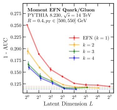
(a)

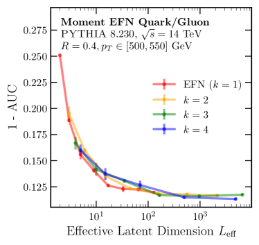
(b)

Figure 1: The performance (AUC) on quark/gluon discrimination of the $k$ Moment EFN as a function of the (a) latent dimension $L$ and (b) effective latent dimension $L_{\mathrm{eff}}$ for different values of $k$. The thin horizontal dashed lines indicate the best value of the AUC achieved. For each model, the spread and mean of the AUC across 3 trainings is shown.

III.2 Performance

Model	AUC	$1/\epsilon_{g}$ at $\epsilon_{q}=0.3$	$1/\epsilon_{g}$ at $\epsilon_{q}=0.5$	Trainable Parameters
$k=1,L=1$ EFN	0.743 $\pm$ 0.001	54.2 $\pm$ 1.7	12.0 $\pm$ 0.1	31106
$k=2,L=1$ Moment EFN	0.802 $\pm$ 0.002	53.9 $\pm$ 3.5	16.7 $\pm$ 0.2	31206
$k=3,L=1$ Moment EFN	0.831 $\pm$ 0.000	52.2 $\pm$ 2.6	18.5 $\pm$ 0.2	31306
$k=4,L=1$ Moment EFN	0.841 $\pm$ 0.004	61.6 $\pm$ 2.8	21.3 $\pm$ 0.1	31406
$k=1,L=4$ EFN	0.843 $\pm$ 0.004	64.0 $\pm$ 2.1	24.5 $\pm$ 1.0	31745
$k=1,L=128$ EFN	0.879 $\pm$ 0.001	69.2 $\pm$ 1.8	31.4 $\pm$ 0.8	89653
$k=2,L=64$ Moment EFN	0.886 $\pm$ 0.001	83.0 $\pm$ 1.3	30.7 $\pm$ 0.6	260085
$k=3,L=32$ Moment EFN	0.886 $\pm$ 0.001	72.6 $\pm$ 2.1	33.6 $\pm$ 1.0	690645
$k=4,L=16$ Moment EFN	0.887 $\pm$ 0.001	81.6 $\pm$ 3.4	32.7 $\pm$ 0.4	517461

Table 1: The AUC and gluon rejection factor at quark efficiencies of 0.3 and 0.5 for the $k=1,2,3$, and $4$ Moment EFNs trained in Sec. III. Here, we show results for the $L=1$ networks, alongside the $k=1,L=4$ ordinary EFN, which achieves comparable results to the $k=4,L=1$ Moment EFN. We also show the highest latent dimension $L$ considered at each order ($L=128,64,32$, and $16$ respectively). For each metric, the model with the best performance is bolded.

For orders $k=1$ through $4$, we train Moment EFNs for a wide range of latent dimensions $L$ from $1$ to $128$ in powers of 2. Due to memory and training time considerations, we consider only up to $L=2^{8-k}$, since otherwise $L_{\mathrm{eff}}$ becomes prohibitively large. For each model, we report its performance using the “area under curve” (AUC) metric across three retrainings. We also report the gluon rejection factor at quark efficiencies of $0.3$ and $0.5$ for the largest $L$ and smallest $L$ models in Table 1 for ease of comparison with other quark/gluon discrimination studies Komiske et al. (2017); ATL (2017); Cheng (2017); Luo et al. (2019); Kasieczka et al. (2019); Komiske et al. (2019b); Lee et al. (2019a, b); Moreno et al. (2020); Qu and Gouskos (2020b); Mikuni and Canelli (2020); Dreyer and Qu (2021); Bogatskiy et al. (2022b); Qu et al. (2022); He and Wang (2023); Dolan et al. (2023). The specific details of the models and training procedure may be found in App. A.

The resulting model performances on the quark/gluon discrimination task, as a function of $L$ and $L_{\mathrm{eff}}$, are shown in Figs. 1a and 1b respectively. From these plots we can make four key observations:

1. At fixed $L$, AUC improves with $k$: As expected, increasing the order of the Moment EFN improves its performance for fixed $L$, since the ansatz is more expressive. This effect is particularly pronounced near $L=1$, with the AUC improving from 0.75 to 0.84 from $k=1$ to $k=4$.

2. Higher $k$ saturates faster: As $k$ increases, the value of $L$ required to saturate performance drops. The ordinary EFN saturates around $L=128$, whereas the order $k=4$ saturates around $L=16$. To achieve peak performance, you don’t need as high an $L$ with a Moment EFN.

3. Peak AUC improves with $k$: The highest AUC achieved by these models improves slightly with $k$, as indicated by the dashed lines in Fig. 1a. In Fig. 1b, we can see that this is primarily driven by the extremely high effective latent dimensions reached by higher $k$ Moment EFNs.

4. $L_{\mathrm{eff}}$ drives performance: The AUC correlates very strongly with $L_{\mathrm{eff}}$, regardless of the order $k$. This suggests that “encoding” and “decoding”, as per Eq. (10), is occurring, and that the quark/gluon discriminant is “compressible” into fewer elementary functions. In particular, if an ordinary EFN requires $L_{\mathrm{eff}}$ latent dimensions to achieve a desired performance in quark/gluon discrimination, an order $k$ Moment EFN would only require $L\sim k!\,L_{\mathrm{eff}}^{1/k}$ latent dimensions to achieve the same performance.

All of these observations point to Moment EFNs being able to achieve the same (or better) performance as ordinary EFNs but with a significantly smaller learned latent space dimension. The quark/gluon discriminator can be efficiently compressed, with the peak classifier going from being composed of $\sim 128$ functions to only $\sim 16$ functions while gaining a slight performance bump in the process. It is also especially remarkable that an order $k=4$ Moment EFN is able to achieve an AUC of 0.84 with just a single latent dimension, equivalent to an ordinary EFN with 4 latent dimensions, and only a few points away from the best possible EFN score of 0.88. We have checked for all studies shown here that going to $k=5$ and beyond does not offer any significant improvement over $k=4$.

Note that these 4 observations are not generically true across different classification tasks: As shown in App. C, the improvement in Observation 1 is not always perfectly monotonic in $k$, and Observation 4 especially is not true for top/QCD jet discrimination – as noted in Sec. II.2, a higher $k$ Moment EFN may be less expressive than a lower $k$ Moment EFN with the same $L_{\mathrm{eff}}$, causing performance to potentially worsen with $k$ for fixed $L_{\mathrm{eff}}$.

IV Opening the Black Box

One practical advantage of the smaller latent dimension afforded by Moment EFNs is that lower dimensional spaces are easier to visualize and interpret. An $L=4$ ordinary EFN involves the complex interplay of 4 independent functions on detector space, whereas the equivalent order $k=4$, $L=1$ Moment EFN achieving the same performance only has a single function to look at (and moreover, we will see that this single function is radially symmetric!). For small $L$, we can even obtain closed form expressions for the latent spaces of Moment EFNs, and due to the effective latent space, we can use this to extend our understanding of ordinary EFNs for larger values of $L$ than we could have otherwise.

The rest of this section proceeds as follows: In Sec. IV.1, we take the order $k=4$, $L=1$ models trained in Sec. III, visualize their internal representations, and find a closed-form expression for their latent spaces, resulting in observables we call “log angularities”. In Sec. IV.2, we show to what extent the $F$ network can also be cast into closed form. Finally, in Sec. IV.3, we briefly discuss $L\geq 2$ models.

IV.1 $L=1$ and Log Angularities

When $L=1$, it is feasible to study exactly what the model learned and extract a single closed-form, one-dimensional observable representing the entire latent space Datta and Larkoski (2018); Komiske et al. (2019a). The order $k=4$, $L=1$ Moment EFN is able to achieve an AUC of 0.84 using a single learned representation, and our goal is to understand and extract this representation. Because of the effective latent space, interpreting the latent space of the order $k=4$, $L=1$ Moment EFN is equivalent to interpreting all four of the latent dimensions of an $L=4$ ordinary EFN. This study is modeled after the study performed in Ref. Komiske et al. (2019a), which constructs two independent observable using an $L=2$ ordinary EFN and achieves an AUC $\sim 0.80$.

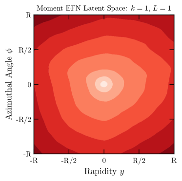
(a)

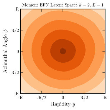
(b)

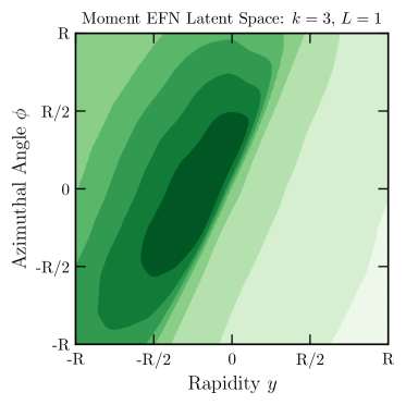
(c)

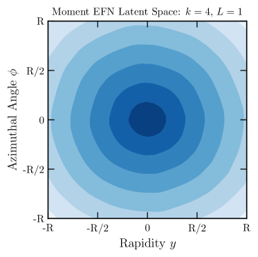
(d)

Figure 2: Examples of learned Moment EFN latent space embeddings $\Phi(x)$, for (a) $k=1$, (b) $k=2$, (c) $k=3$, and (d) $k=4$. Each figure represents the best model of the $L=1$ trainings from Sec. III. The overall normalization is arbitrary. The $k=3$ example features mirror rather than radial symmetry, which can generically occur for $k=2$, $3$, and $4$.

Since $\Phi(x)$ is a function of the rapidity-azimuth plane, we can directly plot the latent spaces of the best $L=1$ networks in 2D following the procedure outlined in Ref. Komiske et al. (2019a), where it is possible to visualize the entire latent space at once. We show examples of this in Fig. 2 for $k=1$ through $4$. We first note that while the $k=1,2$ and $4$ networks learn a radially symmetric latent space, the $k=3$ network does not – it instead exhibits an approximate mirror symmetry. This is not a feature unique to $k=3$, as this mirror symmetric latent space occasionally occurs for $k=2$ and $k=4$ networks as well in some retrainings, though seemingly without loss in performance. Since QCD jets are approximately radially symmetric Ellis et al. (1992); Abe et al. (1993), the fact that this “symmetry breaking” doesn’t affect performance is not surprising, since only radial information is necessary for classification. The precise mechanism that causes this to occur likely is sensitive to the training dynamics of the models.

We now focus our attention to the highest performing models: the order $k=4$ Moment EFNs. In Fig. 3, we show a radial slice of the $k=4,L=1$ latent space (shown fully in Fig. 2d). The radial slice is taken at an azimuthal angle of 0 as a function of the rapidity $y$, though this choice is arbitrary. Even in cases where “symmetry breaking” occurs in the latent space, we find that the radial profile is largely the same up to normalization on any projection not along the mirror symmetry axis. Motivated by the form of the radial profile in Fig. 3, we fit the function:

$$\Phi_{\mathcal{L}}(r)=c_{1}+c_{2}\log(c_{3}+r),$$ (12)

where $r$ is the radial distance in the rapdity-azimuth plane from $(0,0)$, as defined by the energy-weighted average position of the jet.

This function provides an excellent fit to the latent function with $c_{1}=-3.584,c_{2}=-0.847$, and $c_{3}=0.005$. The values of $c_{1}$ and $c_{2}$ are largely unimportant, since they will be subject to affine transformations within the first layer of the $F$ network, and these parameters vary significantly across retrainings. On the other hand, $c_{3}$ is consistently a small number in the range of 0.002 to 0.01, and is embedded in a logarithm which is more nontrivial for $F$ to unravel.

The function $\Phi_{\mathcal{L}}$ has a divergence as $r\to 0$ (i.e. as particles become collinear with the jet center), but this divergence is regulated by the $c_{3}$ parameter. Interestingly, $c_{3}$ is within an $\mathcal{O}(1)$ factor of $\frac{\Lambda_{QCD}}{p_{T}R}\sim 0.001$, suggesting that the nonzero value of $c_{3}$ is due to genuine nonperturbative physics near the jet core learned by the Moment EFN.

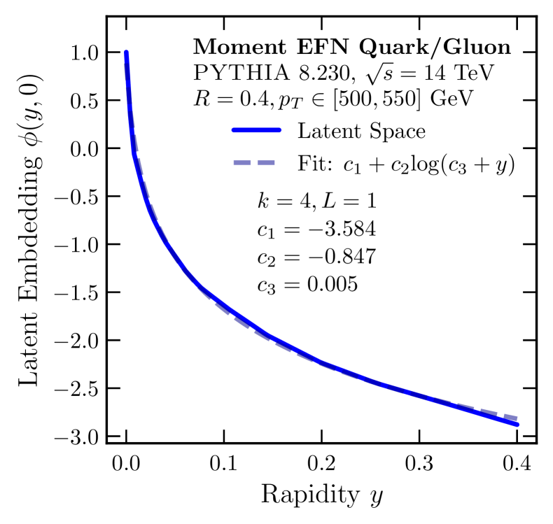
Figure 3: A radial slice of the latent space for the best performing $k=4,L=1$ Moment EFN, as a function of rapidity ($y$). The radial slice is taken at an azimuthal angle of zero. The latent space is shown as a dark blue line, and the logarithmic fit from Eq. (12) is shown as a blue dashed line.

The moments of the function $\Phi_{\mathcal{L}}$ can be used to construct jet shape observables of the form:

$$\mathcal{L}^{(n)}(\mathcal{P}) =\expectationvalue{\Phi_{\mathcal{L}}^{n}}_{\mathcal{P}},$$

$$=\sum_{i\in\mathcal{P}}z_{i}\left(c_{1}+c_{2}\log(c_{3}+r_{i})\right)^{n}.$$ (13)

We call the observables $\mathcal{L}^{(n)}$ log angularities, since they resemble ordinary jet angularities $\lambda^{\beta}(\mathcal{P})=\sum_{i\in\mathcal{P}}z_{i}r_{i}^{\beta}$ for $c_{1}=c_{2}=0$. It is possible to generically set $c_{1}=c_{2}=0$ by taking linear combinations of $\mathcal{L}^{(n)}$ for different $n$, but we elect to keep these parameters as it reduces the amount of total linear transformations our 3 hidden-layer dense networks have to do. These log angularities are interesting observables in their own right, especially in the $c_{3}\to 0$ limit and are closely related to the $\beta\to 0$ limit of ordinary angularities Larkoski et al. (2013); Bright-Thonney et al. (2023), though we save a more in-depth theoretical discussion of log angularities for future work and here focus on their use as quark/gluon taggers.

We can use these analytic observables as inputs to a simple dense neural network classifier of the form:

$$F^{(k)}(\mathcal{L}^{(1)},...,\mathcal{L}^{(k)}).$$ (14)

If the $k=4$ dense neural net classifier has the same performance as the full order $k=4$ Moment EFN, then we can claim not only to have found a fully analytic form of the $k=4$ latent space, but equivalently to have found a fully analytic form of the four different $L=4$ ordinary EFN latent space dimensions.

Model	AUC	$1/\epsilon_{g}$ at $\epsilon_{q}=0.3$	$1/\epsilon_{g}$ at $\epsilon_{q}=0.5$	Trainable Parameters
$k=1$ Log Angularity DNN	0.730 $\pm$ 0.001	50.5 $\pm$ 1.2	8.5 $\pm$ 0.9	$3+20702$
$k=2$ Log Angularity DNN	0.784 $\pm$ 0.001	72.0 $\pm$ 1.7	13.5 $\pm$ 0.8	$3+20802$
$k=3$ Log Angularity DNN	0.816 $\pm$ 0.001	59.9 $\pm$ 1.7	19.4 $\pm$ 1.1	$3+20902$
$k=4$, Log Angularity DNN	0.821 $\pm$ 0.002	55.6 $\pm$ 2.0	18.5 $\pm$ 1.2	$3+21002$
$k=4$, $c_{3}\to 0$ DNN	0.799 $\pm$ 0.001	60.7 $\pm$ 1.8	15.5 $\pm$ 1.0	$2+21002$

Table 2: The same as Table 1, but with dense neural networks on log angularities as defined in Eq. (14). The “$3+$” and “$2+$” in the trainable parameters column refer to the parameters in the log angularity fit.

In Fig. 4, we show ROC curves of the classifier defined by Eq. (14) for $k=1$ through $4$. The $F$ networks used here have precisely the same architecture and training procedure as those used for the Moment EFNs in Sec. III, described in App. A. These results are also summarized in Table 2. We also show, in purple, the $k=4$ DNN classifier taking $c_{3}$ to 0. From this plot, we can make several observations:

1. The $k=4$ dense model is as good as the $k=4$ Moment EFN: We can replace the neural network latent dimension $\Phi(x)$ with the much simpler $\Phi_{\mathcal{L}}(r)$ when $L=1$. Moreover, since the $k=4$, $L=1$ Moment EFN is just as good as the $L=4$ ordinary EFN, the single function $\Phi_{\mathcal{L}}(r)$ and its powers captures the same information as 4 dimensions worth of latent space in an ordinary EFN.

2. The $k=1,2$, and $3$ dense models are not as good as their corresponding order $k$ Moment EFNs: The AUCs of the dense models are slightly lower than the corresponding $L=1$ Moment EFNs in Table 1 for $k<4$. This suggests that while the combination of $\mathcal{L}^{(1)},\mathcal{L}^{(2)},\mathcal{L}^{(3)},\mathcal{L}^{(4)}$ are optimal, individually they are not, and $\mathcal{L}^{(1)}$ by itself is not the most optimal single-variable observable for IRC-safe quark/gluon discrimination.

3. The $c_{3}$ parameter matters: Taking the parameter $c_{3}$ to zero reduces the AUC of the $k=4$ models significantly. Interpreting $c_{3}$ as a nonperturbative parameter regulating a collinear divergence in the logarithm, this loss in performance can be viewed as the learned effect of nonperturbative physics in quark/gluon discrimination.

Thus, at least for $k=4$, we have successfully cast the latent space of not only the Moment EFN, but the equivalent $L=4$ ordinary EFN, into closed form.

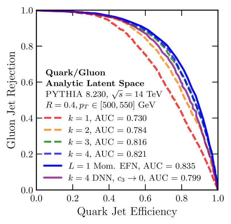
Figure 4: ROC curves showing the performance of the analytic jet shape observables, as defined in Eq. (13), as a quark/gluon classifier. The jet shapes are passed into a dense neural net $F$ as in Eq. (14). The ROC of the original $k=4,L=1$ Moment EFN, from which the fits were derived, is shown in dark blue. Also shown in purple is a variant of the $k=4$ DNN, except where the $c_{3}$ parameter is taken to zero.

IV.2 $L=1$ $F$ Networks

Next, we attempt to go further by attempting to also find closed-form expressions for the dense neural network classifiers $F$, building off of the analysis performed in Sec. IV.1 where we found closed-form expressions for the latent space network $\Phi$. This would result in a fully closed-form quark/gluon jet classifier. However, analyzing $F$ is inherently more difficult than the individual $\Phi$ functions, as for the $k=4$, $L=1$ model of interest, $F$ is a function of 4 inputs. Moreover, we know $F$ must be nontrivial in all 4 inputs, since otherwise there would be no difference between the $L=1$ networks at different values of $k$.

To aid in determining a functional form of $F$, we begin by plotting the output of the dense neural networks (Eq. (14)) considered in Sec. IV.1 as a function of $\mathcal{L}^{(}i)$, for $k=1,\ 2$, and 3. To be explicit, we plot $F^{(1)}(\mathcal{L}^{(1)})$ in Fig. 5a, plot $F^{(2)}(\mathcal{L}^{(1)},\mathcal{L}^{(2)})$ in Fig. 5b, and plot $F^{(3)}(\mathcal{L}^{(1)},\mathcal{L}^{(2)},\mathcal{L}^{(3)})$ in Fig. 5c. We will find it convenient to work with “cumulant” log angularities $\mathcal{L}_{c}$, rather than ordinary log angularities, as this makes the distributions in Fig. 5 and the resulting fits simpler. The cumulant log angularities are defined as:

$$\mathcal{L}_{c}^{(1)} =\mathcal{L}^{(1)},$$ (15)

$$\mathcal{L}_{c}^{(2)} =\mathcal{L}^{(2)}-[\mathcal{L}^{(1)}]^{2},$$ (16)

$$\mathcal{L}_{c}^{(3)} =\mathcal{L}^{(3)}-3\mathcal{L}^{(1)}\mathcal{L}^{(2)}+2[\mathcal{L}^{(1)}]^{3},$$ (17)

$$\mathcal{L}_{c}^{(4)} =\mathcal{L}^{(4)}-4\mathcal{L}^{(1)}\mathcal{L}^{(3)}-3[\mathcal{L}^{(2)}]^{2}$$

$$\quad+12\mathcal{L}^{(2)}[\mathcal{L}^{(1)}]^{2}-6[\mathcal{L}^{(1)}]^{4}.$$ (18)

In all three plots, we see that the DNN output is, for the most part, cleanly divided into distinct regions in $\mathcal{L}_{c}^{(i)}$ space. This motivates using a weighted distance from a learned reference point in $\mathcal{L}_{c}^{(i)}$ space as a classifier, with the ansatz:

$$F^{(k)}(\mathcal{L}^{(1)},...,\mathcal{L}^{(k)})=\sigma\left(w_{0}+\sum_{i=1}^{k}w_{i}\left(\mathcal{L}_{c}^{(i)}-b_{i}\right)^{2}\right),$$ (19)

where $w_{i}$ and $b_{i}$ are parameters to be minimized, and $\sigma$ is the sigmoid function. The number of parameters in this classifier is naively $4+2k$, with 3 from the log angularity fit, 1 from $w_{0}$, and $2k$ from $w_{i}$ and $b_{i}$. However, because any monotonic function of a classifier is an equally good classifier, this can be reduced to $2+2k$ by removing $w_{0}$ and an overall scale from the $w_{i}$’s.

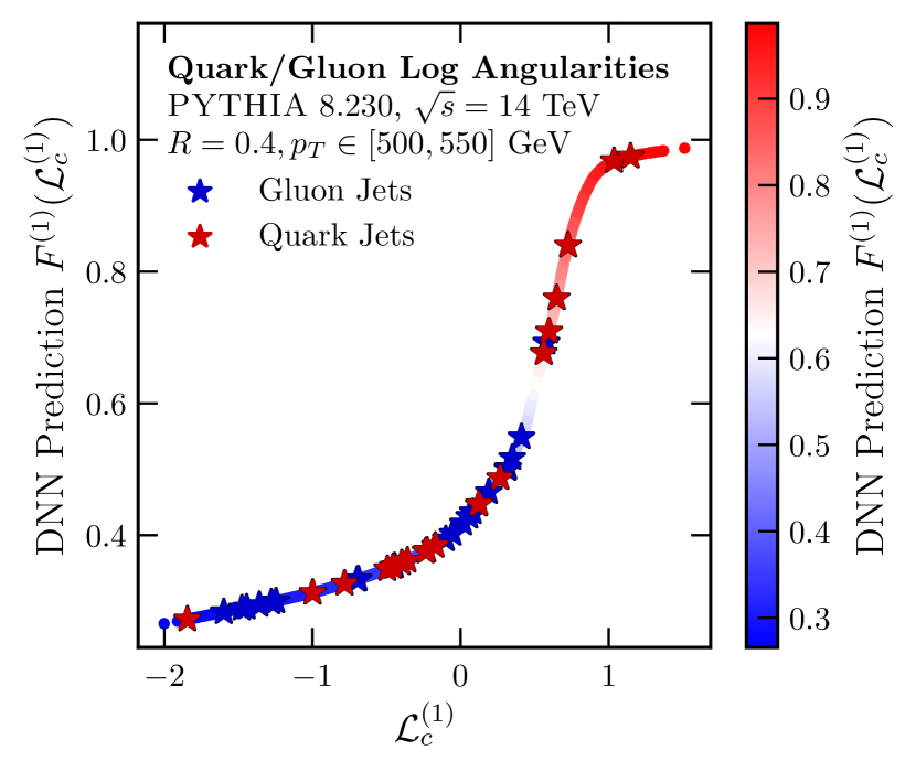
(a)

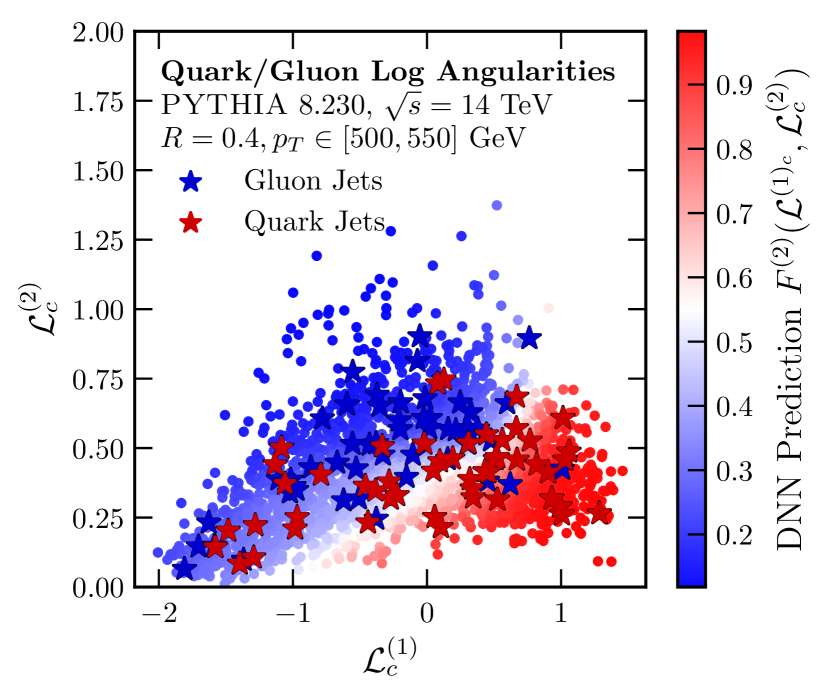
(b)

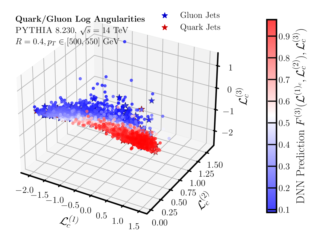
(c)

Figure 5: The distribution of the dense neural network output (a) $F^{(1)}$, (b) $F^{(2)}$, and (c) $F^{(3)}$ as a function of the first, first two, and first three (cumulant) log angularities respectively. The true quark/gluon label for several jets are indicated with colored stars.

Model	AUC	$1/\epsilon_{g}$ at $\epsilon_{q}=0.3$	$1/\epsilon_{g}$ at $\epsilon_{q}=0.5$	Trainable Parameters
$k=1$ Log Angularity Closed Form	0.725 $\pm$ 0.001	36.2 $\pm$ 0.2	7.0 $\pm$ 0.0	$3+1$
$k=2$ Log Angularity Closed Form	0.780 $\pm$ 0.002	57.4 $\pm$ 0.2	10.6 $\pm$ 0.1	$3+3$
$k=3$ Log Angularity Closed Form	0.781 $\pm$ 0.002	57.8 $\pm$ 2.8	12.1 $\pm$ 0.1	$3+5$
$k=4$ Log Angularity Closed Form	0.793 $\pm$ 0.002	54.6 $\pm$ 1.7	12.7 $\pm$ 0.4	$3+7$

Table 3: The same as Table 1, but with the closed-form expressions defined in Eq. (19). The “$3+$” in the trainable parameters column refers to the parameters in the log angularity fit.

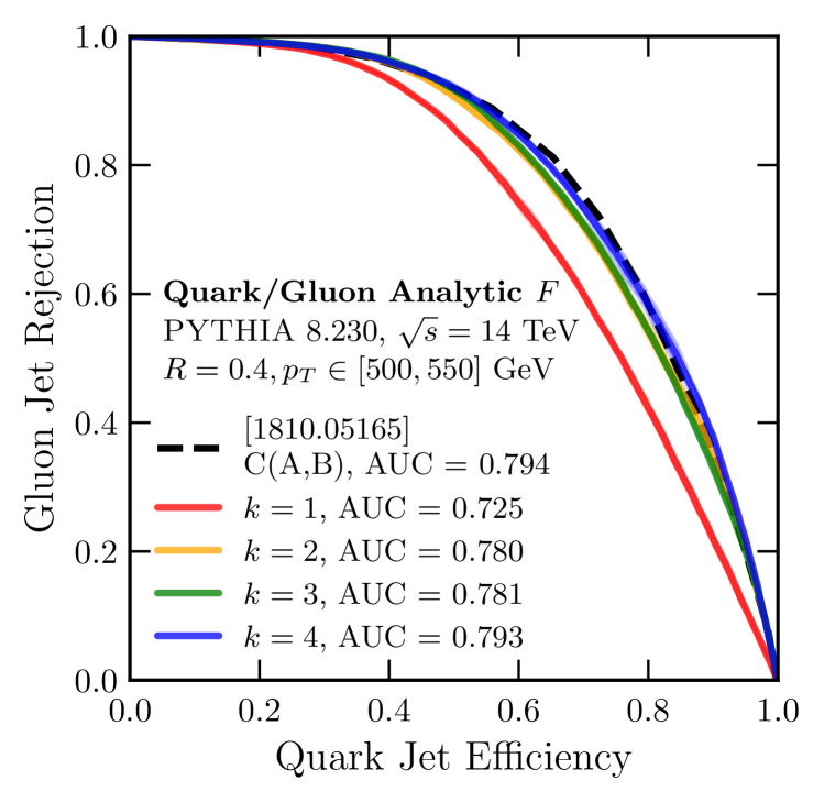
Figure 6: ROC curves showing the performance of the closed form observables, as defined in Eq. (19), as a quark/gluon classifier. For comparison, we also show the ROC curve of the observable $C(A,B)$, a closed-form observable based on fits to an $L=2$ EFN as defined in Ref. Komiske et al. (2019a).

In Fig. 6, we show ROC curves corresponding to the observables defined in Eq. (19). We also summarize these results in Table 3. For $k>1$, the performance saturates around an AUC of $0.78-0.79$, which is roughly the performance of an $L=2$ EFN. Unlike the case where $F$ was a dense network, however, the performance does not improve significantly beyond $k=2$ – moreover, these results are largely uncharged for various modifications to the functional form of Eq. (19), including extending to up to degree $4$ polynomials in $\mathcal{L}$ and $\mathcal{L}_{c}$ and even up to degree $4$ rational polynomials. This suggests that the contributions of higher-order moments beyond the first two are more complex and unable to be easily parameterized – that is, while it is easy to encode the latent space information into a smaller $L$ via Eq. (10), the decoding of the effective latent space in $F$ is nontrivial.

For comparison, we also show the ROC curve of the observable $C(A,B)$, an observable with a similar functional form defined in Ref. Komiske et al. (2019a) based off of fits to an $L=2$ ordinary EFN. This observable also saturates at roughly the same AUC. Thus, while we have succeeded in developing a fully closed-form solution suitable for up to $k=2$, equivalent to 2 latent dimensions of an ordinary EFN, finding a closed form expression for $F$ beyond 2 effective latent dimensions is nontrivial.

IV.3 Beyond $L=1$

Finally, we briefly look at Moment EFNs with $L>1$ to see if we can attempt to gain some insight into them, just like the $L=1$ Moment EFNs. Unlike the case with $L=1$ Moment EFNs, the analysis of $L>1$ models is much more difficult, both due to the higher dimension and because the product structure allows radial symmetry to be more easily broken, even for $L=2$.

In order to visualize the latent spaces for $L>1$, we follow the procedure outlined in Ref. Komiske et al. (2019a). We can overlay all $L$ learned $\Phi$ functions of each model at once by drawing the $45\%-55\%$ contours of each $\Phi$ function. In these plots, the overall normalization and sign of the $\Phi$ functions is unimportant, as the $F$ network easily learn to rescale its inputs via simple linear transformations. As an example, in Fig. 7, we show the $L=128,64,32,$ and $16$ (the highest $L$ considered for each $k$) dimensional latent spaces of the highest performing models for the order $k=1,2,3,$ and $4$ Moment EFNs, respectively. Like the EFN, the Moment EFN is able to pick up on the collinear singularity of QCD, as filters closer to the center are more closely resolved. Note that while on the whole, the entire ensemble of contours appears to be radially symmetric, the individual contours are not – this in contrast with the $L=1$ Moment EFNs, where the $\Phi$ functions were genuinely radially symmetric (or at the very least, broken to mirror symmetric).

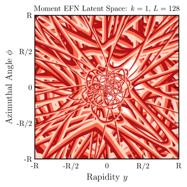
(a)

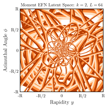
(b)

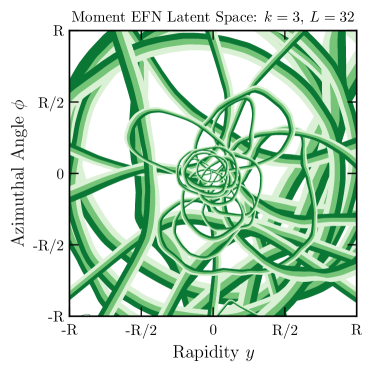
(c)

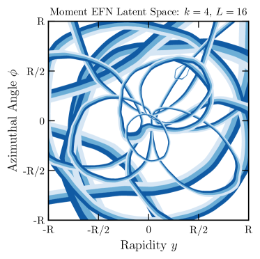
(d)

Figure 7: The contours of the learned Moment EFN latent space embeddings $\Phi$, for (a) $k=1$, (b) $k=2$, (c) $k=3$, and (d) $k=4$. Each figure represents the best model for the highest value of $L$ considered for each $k$: 128, 64, 32, and 16 respectively. Each curve represents the $45\%-55\%$ contours of each of the $L$ different $\Phi$ functions. The overall normalization is arbitrary.

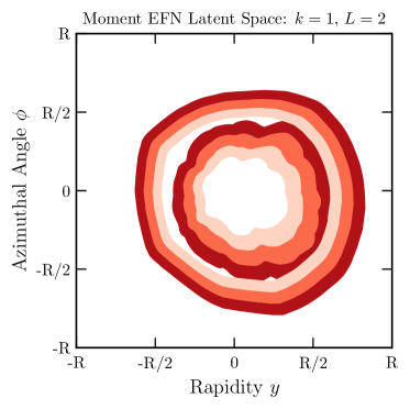
(a)

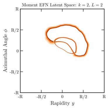
(b)

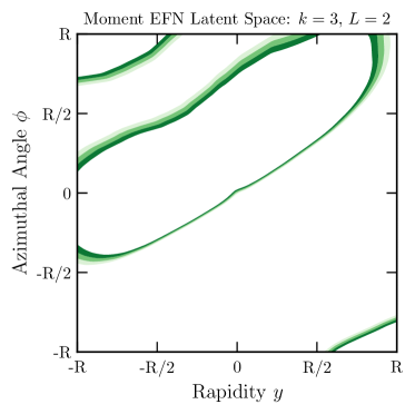
(c)

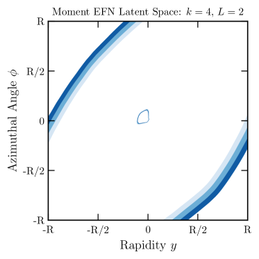
(d)

Figure 8: The contours of the learned $L=2$ Moment EFN latent space embeddings $\Phi$, for (a) $k=1$, (b) $k=2$, (c) $k=3$, and (d) $k=4$. Each curve represents the $45\%-55\%$ contours of each of the 2 different $\Phi$ functions. The overall normalization is arbitrary.

After $L=1$ from Fig. 2, the next most natural thing to study are the $L=2$ latent spaces, which we show in Fig. 8. Not only is $L=2$ less radially symmetric than $L=1$ in general, we also notice the $k>1,L=2$ Moment EFNs exhibit less radial symmetry than the $L=2$ ordinary EFN. With product structures, it is easier to form nontrivial representations of the rotation group that later combine to form the trivial representation. As an example, the functions $\Phi^{1}(x)=x^{(1)}$ and $\Phi^{2}(x)=x^{(2)}$ are themselves not radially symmetric, but the $k=2$ moment combination $F(\Phi)=(\Phi^{1})^{2}+(\Phi^{2})^{2}$ is. Nevertheless, some models occasionally still seem to retain some approximate radial symmetry, as is the case for the order $k=4$ model in Fig. 8d.

We now move to analyze and fit the radial projections of the order $k=4,L=2$ Moment EFN in hopes of finding closed-form expressions for the (now two) latent dimensions, exactly as was done in Sec. IV.1. This model has $L_{\mathrm{eff}}=15$, which is roughly equivalent to an ordinary EFN with 14 latent dimensions – in principle, fitting these two functions should therefore enable us to extract the same information as 14 latent dimensions worth of information in an ordinary EFN by taking moments. These radial projections are shown in Fig. 9. One of the two latent dimensions takes the form of a log angularity, as defined in Eq. (13), and the $c_{3}$ parameter is also in the expected range. We will call the associated jet shape observable $\mathcal{L}^{\prime}$, with the prime indicative of the slightly different values of the fit parameters $c_{i}$. For the second latent dimension, we fit the form:

$$\Phi_{\mathcal{E}}(r)=d_{1}+d_{2}\exp(-r^{2}/d_{3}^{2}),$$ (20)

motivated both by the form of the plot and the use of a similar form in the analysis of the $L=2$ EFN in Ref. Komiske et al. (2019a). Just as with log angularities, we can define moment-based jet shape observables based off this fit, which we will denote $\mathcal{E}^{(n)}$, and associated cumulants $\mathcal{E}^{(n)}_{c}$. We can also define mixed moments $\mathcal{M}^{(mn)}$ of the form $\mathcal{M}^{(mn)}\equiv\expectationvalue{\Phi_{\mathcal{L}^{\prime}}^{m}\Phi_{\mathcal{E}}^{n}}$.

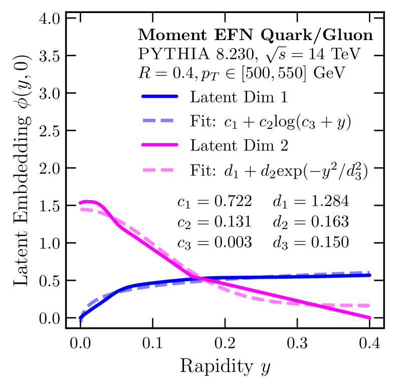
Figure 9: The same as Fig. 3, but for the best performing $k=4,L=2$ Moment EFN. The two latent dimensions are shown in blue and pink.

We can use the observables $\mathcal{L}^{\prime(n)}$ and $\mathcal{E}^{(n)}$ as inputs to dense neural networks $F$ as a measure of how well the latent spaces are approximated by these fits. Here, the dense network $F^{(k)}$ takes in all $L_{\mathrm{eff}}(k)$ multivariate moments of the two observables – for instance, the $k=2$ dense network has the form $F^{(2)}({\mathcal{L}^{\prime}}^{(1)},\mathcal{E}^{(1)},{\mathcal{L}^{\prime}}^{(2)},\mathcal{E}^{(2)},\mathcal{M}^{1,1})$. We show the performance of these networks in Fig. 10a. We see here that unlike the $L=1$ analysis performed in Sec. IV.1, the two observables here are not enough to reproduce the full $L=2$, $k=4$ Moment EFN – in fact, they are only about as good as the $L=1$, $k=4$ result at best. This means that the fits are not enough to capture the full latent space, suggesting that non radially symmetric information is important.

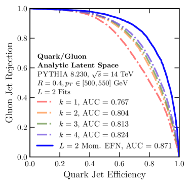
(a)

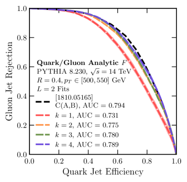
(b)

Figure 10: (a) The same as Fig. 4, but with the $L=2$ fits and dense networks. (b) The same as Fig. 6, but for the closed-form $F$ defined using $L=2$ in Eq. (21).

Finally, as was done in Sec. IV.2, we may attempt to build closed-form taggers from these fits. To accommodate the second observable, we extend the form of our fit to:

$$F^{(k)}(\mathcal{L}^{(i)},\mathcal{E}^{(i)})=\sigma\bigg{(} w_{0}+\sum_{i=1}^{k}w^{\mathcal{L}^{\prime}}_{i}\left(\mathcal{L}_{c}^{(i)}-b_{i}^{\mathcal{L}^{\prime}}\right)^{2}$$

$$+\sum_{i=1}^{k}w^{\mathcal{E}}_{i}\left(\mathcal{E}_{c}^{(i)}-b_{i}^{\mathcal{E}}\right)\bigg{)}.$$ (21)

For simplicity, we have not considered mixed moments between the two observables. We show the performance of these taggers in Fig. 10b. The observables here are no better than the $L=1$ analytic observables shown in Fig. 6 – in fact, they are slightly worse, due to the extra numerical cost of optimizing additional parameters. That us, unlike the EFN observable $C(A,B)$, the additional parameterization power granted by an additional latent dimension in a Moment EFN is more complex than can be captured by a simple functional dependence.

V Conclusions and Outlook

In this paper, we presented an extension of the Deep Sets framework in the form of Moment Pooling. Moment Pooling arises when the summation operation in Deep Sets is generalized to arbitrary multivariate moments. We have shown an implementation of Moment Pooling in Moment EFNs, a particular Deep Sets framework useful in particle physics. For a fixed number of latent dimensions $L$, an order $k$ Moment EFN is able to reach a much higher effective latent dimension by recycling the same $L$ functions in product structures, and conversely, a Moment EFN is capable of reducing the $L$ required to achieve the same performance as an ordinary EFN.

We find that Moment EFNs are able to achieve the same (or better) performance as ordinary EFNs for quark/gluon discrimination, but with significantly fewer latent dimensions. In particular, an order $k=4$ Moment EFN with only 16 latent dimensions is able to achieve slightly better performance than an EFN with 128 latent dimensions, indicative of “data compression” and structure in the quark/gluon discrimination task. Similarly, an order $k=4$ Moment EFN with only a single latent dimension is able to achieve an AUC of 0.84, equivalent to an ordinary EFN with 4 latent dimensions. By analyzing the latent space of this model, we are able to find a simple, closed-form expression in the form of the log angularity shape observable, whose moments contain the same information as 4 latent dimensions of an ordinary EFN. However, we find that analyzing the $F$ network in closed-form is difficult, and that simple parameterizations cannot go beyond the performance of up to an $L=2$ model, which suggests some complexity in the way the information in log angularities is decoded.

We conclude by discussing possible avenues of further study. One can ask if the latent space structure granted by the moment architecture helps in learning richer jet representations – that is, if the latent representation is a genuine representation of a jet from which multiple attributes and observables can be estimated, not just a quark/gluon discriminant. The latent spaces of EFNs are highly degenerate, and as we have seen, the 4 latent dimensions of an $L=4$ EFN may be replaced by 4 moments of log angularities without any loss of performance on quark/gluon tagging. Second, we have only considered moments, in the sense that we have restricted our architecture to only have terms of the form $\sum_{i\in\mathcal{P}}z_{i}(\Phi^{1}(x_{i}))^{w_{1}}(\Phi^{2}(x_{i}))^{w_{2}}...(\Phi^{L}(x_{i}))^{w_{L}}$, for pre-determined positive integers $w_{l}$ such that $\sum_{l}w_{l}\leq k$. One could imagine generalizing this even further, for example by letting the powers $w_{l}$ be real and negative, or even learned.

The Moment Pooling operation and Moment EFN are a step towards generalizing existing models while adding to their interpretability. We look forward to further developments in the direction of flexible models with interpretable internal representations.

Code and Data

The general Moment EFN, along with several variations (including cumulant-based models and Moment PFNs), is available at https://github.com/athiso/moment. The code used to perform all the analyses and make all the figures featured in this paper is available at https://github.com/rikab/MomentAnalysis in the form of Jupyter notebooks Kluyver et al. (2016).

Appendix A Model and Training Specifications

In this appendix, we provide details for the models and training procedures used in Sec. III and App. C. All models are implemented as modified versions of the EFN/PFN models in the EnergyFlow Python package Komiske et al. (2019a), built with Keras Chollet (2017) using the TensorFlow Abadi et al. (2016) backend. Each training is performed using an NVIDIA A100.

The key difference between the Moment EFN and the ordinary EFN is the addition of the MomentPooling layer between the $\Phi$ and $F$ functions. The MomentPooling layer is a deterministic function $\mathbb{R}^{L}\xrightarrow[]{}\mathbb{R}^{L_{\mathrm{eff}}}$, where $L_{\mathrm{eff}}$ depends on both $L$ and the order $k$, that maps the $L$-component $\Phi$ to the list of all multivariate moments up to order $k$, taken over the event $\mathcal{P}$:

$$\Phi^{a}\mapsto\left(\expectationvalue{\Phi^{a}}_{\mathcal{P}},\expectationvalue{\Phi^{a_{1}}\Phi^{a_{2}}}_{\mathcal{P}},...\expectationvalue{\Phi^{a_{1}}...\Phi^{a_{k}}}_{\mathcal{P}}\right).$$ (22)

Implementation-wise, the MomentPooling layer takes in a TensorFlow tensor of shape $(N_{\text{batch}},N_{\text{particles}},L)$, where $N_{\text{batch}}$ is the number of events to be computed in parallel, $N_{\text{particles}}$ is the maximum number of particles per event, and $L$ is the latent dimension – this tensor is obtained as the output of the $\Phi$ network. The moments are then computed recursively: We first define the $k=0$ moment tensor, a tensor of shape $(N_{\text{batch}},N_{\text{particles}},1)$ with every entry equal to 1. Given the $k$’th moment tensor, which is of shape $(N_{\text{batch}},N_{\text{particles}},L_{\mathrm{eff}}(k))$, the $k+1$’th moment tensor is obtained by performing the outer product of the original input tensor, to obtain a new tensor of shape $(N_{\text{batch}},N_{\text{particles}},L_{\mathrm{eff}}(k),L)$. Note that this outer product will contain redundant moments, since the order of indices does not matter – thus, we only perform the outer product on the indices corresponding to the upper triangular part of the $k+1$-dimensional hypercube with $L$ indices per dimension. The tensor is then flattened and concatenated to the $k$’th moment tensor to form the $k+1$’th moment tensor of shape $(N_{\text{batch}},N_{\text{particles}},L_{\mathrm{eff}}(k+1))$. At the end of the recursive procedure, we perform the $z$-weighted sum over the $N_{\text{particles}}$ dimension, so that the final output has shape $(N_{\text{batch}},L_{\mathrm{eff}}(k))$. This recursive procedure allows for some computations to be reused when computing higher-order moments, simplifying the TensorFlow computational graphs and saving time on backpropagation versus recomputing all moments from scratch.

Following Ref. Komiske et al. (2019a), all of our models consist of a $\Phi$ network with three layers of sizes $100$, $100,$ and $L$ respectively (with $L$ being the latent dimension), and an $F$ network with four layers of size $100,100,100,$ and $1$ respectively. For both networks, the final layer is the output layer. In between $\Phi$ and $F$ is the MomentPooling layer. We use LeakyReLU Maas (2013) with $\alpha=0.3$ for all activation functions, except for the final layer of $F$, where we use a sigmoid function for the classifier output.

To aid our models in learning efficient representations, especially for $k>1$, we use a “pre-training” procedure. This procedure helps to ensure that each additional moment added is used to learn “new” information that helps the model and to mitigate the effect of more nontrivial training for higher order $k$ Moment EFNs. To train an order $k$ Moment EFN, first, we first train order $k-1$ Moment EFN with the exact same value of $L$ and the same hyperparameters for the $\Phi$ and $F$ networks, using the training procedure defined below. Then, we initialize an order $k$ network whose $\Phi$ and $F$ weights are identical to the order $k-1$ model’s weights, except for the weights attached to the MomentPooling layer, as the size of this layer has changed. The weights connecting the first $L_{\mathrm{eff}}(k-1)$ outputs of the MomentPooling layer to the first $F$ layer are the same as the $k-1$ network weights. Finally, the order $k$ model can be trained. This pretraining procedure is recursive: to train the order $k-1$ model, we initialize its weights from an order $k-2$ model, and so on. The weights of the $k=1$ models, plus all other undetermined weights (namely the rest of the weights connecting the MomentPooling layer to the first $F$ layer) are initialized using the default He-uniform He et al. (2015) distribution. To ensure that any improvements are not the result of having more epochs to train, in our comparative studies lower $k$ models have the training procedure described below applied to them multiple times so that all models train for the same total number of epochs.

Each model is trained for 50 epochs with a batch size of 512 – we allow for early stopping with a patience parameter of 8, though early stopping never occurred in any of our trainings. We use 1M total jets for training, 50k for validation, and 50k for testing. We train to minimize the binary crossentropy loss using the Adam optimizer Kingma and Ba (2017) with a learning rate of $0.001$. The training times of each network per epoch on an NVIDIA A100 are shown in Table 4. Each model is re-initialized and re-trained 3 times, the ROC curves and AUC saved for each of the trainings. Note that we do not train models with both larger $k$ and larger $L$, as the training time and memory requirements become excessive.

Latent Dim. $L$	EFN	$k=2$	$k=3$	$k=4$
$2^{0}$	2s	3s	3s	4s
$2^{1}$	3s	3s	3s	4s
$2^{2}$	3s	3s	4s	5s
$2^{3}$	3s	4s	6s	11s
$2^{4}$	3s	6s	16s	66s
$2^{5}$	4s	13s	91s
$2^{6}$	4s	38s
$2^{7}$	5s

Table 4: The time per epoch, in seconds, for the $k=1$ through $4$ Moment EFNs to train on the quark/gluon discrimination dataset.

Appendix B Regression with Jet Angularities

In this appendix, we demonstrate the improved performance and reduced complexity of Moment EFNs in regression tasks by exploring their relationship to jet angularities Berger et al. (2003); Berger and Magnea (2004).

Jet angularities are well-studied QCD observables that quantify the radial distribution of energy within a jet. The product structure of the Moment EFN is especially suited for angularities, since a jet angularity can be thought of as an energy-weighted radial moment. For a jet $\mathcal{P}$, the $\beta$-angularity of the jet, $\lambda^{(\beta)}$, is defined as:

$$\lambda^{(\beta)}(\mathcal{P})\equiv\sum_{i\in\mathcal{P}}z_{i}|x_{i}|^{\beta},$$ (23)

where $x_{i}=(y_{i},\phi_{i})$ are the particle coordinates defined from an appropriately defined jet center $x_{0}$, which we will take to be the energy-weighted average position of the jet.

In the language of moments, jet angularities take a very natural form:

$$\lambda^{(\beta)}(\mathcal{P})=\expectationvalue{|x_{i}|^{\beta}}.$$ (24)

If $\beta$ is an even integer, then $\lambda^{(\beta)}$ can be expressed using a completely linear Moment EFN with $k=\beta$ and $L=2$:

$$\Phi^{1}(x_{i}) =y_{i},\quad\Phi^{2}(x_{i})=\phi_{i},$$ (25)

$$F(\expectationvalue{\Phi}_{\mathcal{P}}) =\sum_{a_{1}=1}^{2}...\sum_{a_{\beta/2}=1}^{2}\expectationvalue{\left(\Phi^{a_{1}}\right)^{2}...\left(\Phi^{a_{\beta/2}}\right)^{2}}_{\mathcal{P}},$$ (26)

where $a=1,2$ corresponds to the two dimensions of $x$. In particular, for $\beta=2$, this becomes:

$$F(\expectationvalue{\Phi}_{\mathcal{P}}) =\expectationvalue{y^{2}}+\expectationvalue{\phi^{2}}.$$ (27)

The $\beta=2$ angularity is especially nice, as it relates to the jet mass:

$$\lambda^{(2)}\approx\frac{m_{J}^{2}}{(\sum E_{i})^{2}}.$$ (28)

The fact that angularities can be represented as a linear function of moments is significant, as dense neural networks, especially those using variants of ReLU, are at their core are piecewise-linear approximators. The nonlinear part of the angularities, namely the $|x|^{\beta}$ function, is encoded in the pre-specified moment functions, leaving only a purely linear function to learn. Thus, one would expect a strictly linear Moment EFN to learn even integer $\beta$ angularities exactly (that is, with a mean squared error loss of zero) for $k\geq\beta$, and in general that $k>1$ Moment EFNs outperform $k=1$ EFNs on generic regression tasks.

To illustrate the improved performance of the Moment EFN on regression tasks, we train $L=2$ Moment EFNs from $k=1$ through $4$ to learn the angularity $\lambda^{(\beta)}$, for values of $\beta\in[0,4]$. The Moment EFNs are strictly linear: The functions $\Phi$ and $F$ are strictly linear functions from $\mathbb{R}^{2}\xrightarrow{}\mathbb{R}^{L}$ and $\mathbb{R}^{L_{\mathrm{eff}}}\xrightarrow{}\mathbb{R}$, respectively, with no hidden layers, activation functions, or even layer biases. We use the exact same quark/gluon dataset described above in Sec. III.1 for this study, though we ignore the quark/gluon label. On each jet, we compute the $\beta$-angularity as defined in Eq. (23), for $\beta$ from $0$ to $4$ in increments of $\Delta\beta=\frac{1}{6}$. The models are trained to minimize the mean-squared error (MSE) over the training set.

In Fig. 11, we plot the average MSE of each model, taken over the three retrainings, on the test set as a function of $\beta$. First, we note that the $k>1$ models are consistently better than the $k=1$ model for $\beta>0$. Second, there are large downward spikes in the loss: at $\beta=0$ for all models; at $\beta=2$ for $k=2$, $3$, and $4$; and at $\beta=4$ for $k=4$. The first two spikes are especially close to zero, with an MSE loss of $\sim 10^{-12}$ approaching floating point precision. This is precisely the behavior expected by Eq. (26), as the linear model is able to achieve an exact (up to machine precision) fit for even integer $\beta$ with $k\geq\beta$.

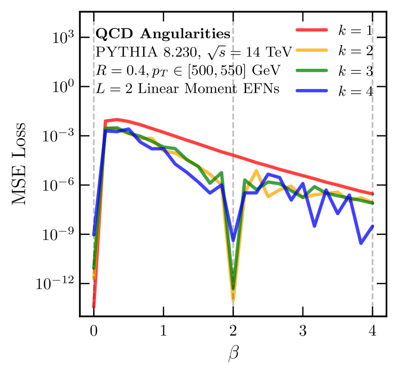
Figure 11: The (average) MSE loss of the $k$ Moment EFN trained to regress the jet angularity $\lambda^{(\beta)}$ as a function of $\beta$. Each line is the average of the MSE across three retrainings.

Appendix C Additional Collider Classification Studies

In this appendix, we present additional studies to supplement Sec. III, both by replacing the EFN in the moment architecture with a PFN, and by replacing the quark/gluon discrimination task with a top/QCD jet discrimination task.

The Moment PFN models are identical to those described in App. A, except $\Phi$ is now a function of the particle $(z_{i},x_{i})$ rather than just $x_{i}$, and $\Phi$ is no longer weighted by $z$. Importantly, this changes the definition of the moment pooling operation, since, as shown in Eq. (8) moments are not energy-weighted.

For our top/QCD dataset, we use the same top-tagging set as in Refs. Butter et al. (2018, 2019), commonly used as a benchmark in tagger studies. This set consists of a top quark jet signal and a mixed light quark and gluon jet background, generated in Pythia 8.2.15 Sjostrand et al. (2006); Sjöstrand et al. (2015) at 14 TeV, and passed through the Delphes 3.3.2 de Favereau et al. (2014) ATLAS detector simulation. The jets are clustered using the anti-$k_{T}$ algorithm Cacciari et al. (2008) with $R=0.8$, and satisfy $p_{T}\in[550,650]$ GeV and $|y|\leq 2$. We do not perform any additional preprocessing here – in particular, we do not rotate the jets in the rapidity-azimuth plane for these studies.

In Figs. 12–14, we show the AUC as a function of latent dimension and effective latent dimension for quark/gluon tagging with Moment PFNs, top tagging with Moment EFNs, and top tagging with Moment PFNs respectively. These figures are meant to complement Figs. 1a and 1b for quark/gluon tagging with Moment EFNs. We also summarize the results of these classifiers in Tables 5–7 for ease of comparison with other studies using the same datasets.

We first observe that $k\geq 2$ architectures perform the same or better as their $k=1$ counterparts for a given value of $L$, though this improvement is not always monotonic. Second, unlike the quark/gluon Moment EFNs, performance per effective latent dimension is not independent of $k$. For the quark/gluon Moment PFNs, the performance per effective latent dimension tends to increase with $k$, but for the top/QCD Moment EFNs and Moment PFNs, the performance per effective latent dimension tends to decrease with $k$. This would seem to imply that the top/QCD discriminant is not “compressible”, in that its latent space cannot be easily factorized into products of just a few functions, and that many independent functions are genuinely required.

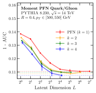
(a)

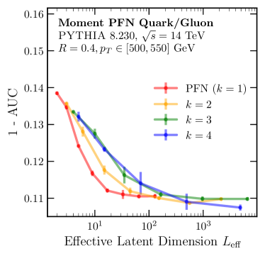
(b)

Figure 12: The same as Figs. 1a and 1b, but with a Moment PFN rather than a Moment EFN.

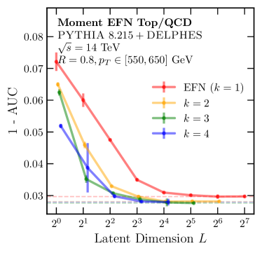
(a)

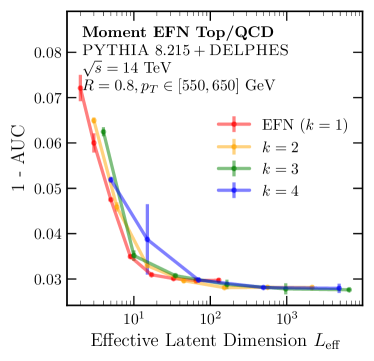
(b)

Figure 13: The same as Figs. 1a and 1b, but with the top/QCD dataset rather than the quark/gluon dataset.

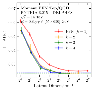
(a)

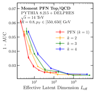
(b)

Figure 14: The same as Figs. 1a and 1b, but with a Moment PFN rather than a Moment EFN and the top/QCD dataset rather than the quark/gluon dataset.

Model	AUC	$1/\epsilon_{g}$ at $\epsilon_{q}=0.3$	$1/\epsilon_{g}$ at $\epsilon_{q}=0.5$	Trainable Parameters
$k=1,L=1$ PFN	0.862 $\pm$ 0.000	50.8 $\pm$ 1.0	19.4 $\pm$ 0.2	31206
$k=2,L=1$ Moment PFN	0.864 $\pm$ 0.001	55.7 $\pm$ 0.9	20.3 $\pm$ 0.1	31306
$k=3,L=1$ Moment PFN	0.866 $\pm$ 0.001	60.9 $\pm$ 2.3	21.3 $\pm$ 0.5	31406
$k=4,L=1$ Moment PFN	0.867 $\pm$ 0.002	62.8 $\pm$ 1.2	22.0 $\pm$ 0.2	31506
$k=1,L=128$ PFN	0.889 $\pm$ 0.002	76.9 $\pm$ 0.6	31.6 $\pm$ 0.5	89753
$k=2,L=64$ Moment PFN	0.890 $\pm$ 0.001	83.0 $\pm$ 1.3	32.2 $\pm$ 1.4	260185
$k=3,L=32$ Moment PFN	0.890 $\pm$ 0.000	76.4 $\pm$ 2.7	33.2 $\pm$ 0.4	690745
$k=4,L=16$ Moment PFN	0.893 $\pm$ 0.001	78.4 $\pm$ 4.0	34.1 $\pm$ 0.8	517561

Table 5: The same as Table 1, but with a Moment PFN rather than a Moment EFN.

Model	AUC	$1/\epsilon_{QCD}$ at $\epsilon_{top}=0.3$	$1/\epsilon_{QCD}$ at $\epsilon_{top}=0.5$	Trainable Parameters
$k=1,L=1$ EFN	0.922 $\pm$ 0.002	29.5 $\pm$ 0.7	16.8 $\pm$ 0.3	31106
$k=2,L=1$ Moment EFN	0.930 $\pm$ 0.002	37.6 $\pm$ 0.6	20.2 $\pm$ 0.4	31206
$k=3,L=1$ Moment EFN	0.933 $\pm$ 0.001	41.2 $\pm$ 2.3	20.6 $\pm$ 0.6	31306
$k=4,L=1$ Moment EFN	0.946 $\pm$ 0.001	70.3 $\pm$ 5.8	29.1 $\pm$ 1.1	31406
$k=1,L=128$ EFN	0.970 $\pm$ 0.000	465.0 $\pm$ 40.0	108.8 $\pm$ 2.4	89653
$k=2,L=64$ Moment EFN	0.972 $\pm$ 0.001	407.9 $\pm$ 16.7	131.0 $\pm$ 3.5	260085
$k=3,L=32$ Moment EFN	0.974 $\pm$ 0.000	416.1 $\pm$ 40.0	138.4 $\pm$ 11.7	690645
$k=4,L=16$ Moment EFN	0.972 $\pm$ 0.001	579.3 $\pm$ 118.4	132.2 $\pm$ 8.2	517461

Table 6: The same as Table 1, but with the top/QCD dataset rather than the quark/gluon dataset.

Model	AUC	$1/\epsilon_{QCD}$ at $\epsilon_{top}=0.3$	$1/\epsilon_{QCD}$ at $\epsilon_{top}=0.5$	Trainable Parameters
$k=1,L=1$ PFN	0.937 $\pm$ 0.001	43.3 $\pm$ 0.5	25.1 $\pm$ 0.1	31206
$k=2,L=1$ Moment PFN	0.944 $\pm$ 0.000	59.8 $\pm$ 0.7	29.0 $\pm$ 0.2	31306
$k=3,L=1$ Moment PFN	0.944 $\pm$ 0.001	62.8 $\pm$ 1.3	29.1 $\pm$ 0.9	31406
$k=4,L=1$ Moment PFN	0.944 $\pm$ 0.000	62.2 $\pm$ 0.4	30.4 $\pm$ 0.9	31506
$k=1,L=128$ PFN	0.975 $\pm$ 0.001	351.8 $\pm$ 12.5	138.8 $\pm$ 7.0	89753
$k=2,L=64$ Moment PFN	0.976 $\pm$ 0.001	303.2 $\pm$ 26.9	156.4 $\pm$ 11.1	260185
$k=3,L=32$ Moment PFN	0.975 $\pm$ 0.000	321.2 $\pm$ 0.0	136.1 $\pm$ 6.2	690745
$k=4,L=16$ Moment PFN	0.976 $\pm$ 0.001	351.8 $\pm$ 12.5	146.0 $\pm$ 17.0	517561

Table 7: The same as Table 1, but with a Moment PFN rather than a Moment EFN and the top/QCD dataset rather than the quark/gluon dataset.

References

- Chakraborty et al. (2017) Supriyo Chakraborty, Richard Tomsett, Ramya Raghavendra, Daniel Harborne, Moustafa Alzantot, Federico Cerutti, Mani Srivastava, Alun Preece, Simon Julier, Raghuveer M. Rao, Troy D. Kelley, Dave Braines, Murat Sensoy, Christopher J. Willis, and Prudhvi Gurram, “Interpretability of deep learning models: A survey of results,” in 2017 IEEE SmartWorld, Ubiquitous Intelligence & Computing, Advanced & Trusted Computed, Scalable Computing & Communications, Cloud & Big Data Computing, Internet of People and Smart City Innovation (SmartWorld/SCALCOM/UIC/ATC/CBDCom/IOP/SCI) (2017) pp. 1–6.
- Gilpin et al. (2018) Leilani H. Gilpin, David Bau, Ben Z. Yuan, Ayesha Bajwa, Michael Specter, and Lalana Kagal, “Explaining explanations: An overview of interpretability of machine learning,” (2018).
- Zhang et al. (2021) Yu Zhang, Peter Tino, Ales Leonardis, and Ke Tang, “A survey on neural network interpretability,” IEEE Transactions on Emerging Topics in Computational Intelligence 5, 726–742 (2021).
- Molnar et al. (2020) Christoph Molnar, Giuseppe Casalicchio, and Bernd Bischl, “Interpretable machine learning – a brief history, state-of-the-art and challenges,” in Communications in Computer and Information Science (Springer International Publishing, 2020) p. 417–431.
- Rudin et al. (2021) Cynthia Rudin, Chaofan Chen, Zhi Chen, Haiyang Huang, Lesia Semenova, and Chudi Zhong, “Interpretable machine learning: Fundamental principles and 10 grand challenges,” (2021), arXiv:2103.11251 [cs.LG] .
- Dillon et al. (2021) Barry M. Dillon, Gregor Kasieczka, Hans Olischlager, Tilman Plehn, Peter Sorrenson, and Lorenz Vogel, “Symmetries, Safety, and Self-Supervision,” (2021), arXiv:2108.04253 [hep-ph] .
- Bogatskiy et al. (2022a) Alexander Bogatskiy et al., “Symmetry Group Equivariant Architectures for Physics,” in 2022 Snowmass Summer Study (2022) arXiv:2203.06153 [cs.LG] .
- Gao and Guan (2023) Lei Gao and Ling Guan, “Interpretability of machine learning: Recent advances and future prospects,” (2023), arXiv:2305.00537 [cs.MM] .
- Bogatskiy et al. (2023) Alexander Bogatskiy, Timothy Hoffman, David W. Miller, Jan T. Offermann, and Xiaoyang Liu, “Explainable Equivariant Neural Networks for Particle Physics: PELICAN,” (2023), arXiv:2307.16506 [hep-ph] .
- Wayland et al. (2024) Jeremy Wayland, Corinna Coupette, and Bastian Rieck, “Mapping the multiverse of latent representations,” (2024), arXiv:2402.01514 [cs.LG] .
- Denby (1988) Bruce H. Denby, “Neural Networks and Cellular Automata in Experimental High-energy Physics,” Comput. Phys. Commun. 49, 429–448 (1988).
- Guest et al. (2018) Dan Guest, Kyle Cranmer, and Daniel Whiteson, “Deep Learning and its Application to LHC Physics,” (2018), 10.1146/annurev-nucl-101917-021019, arXiv:1806.11484 [hep-ex] .
- Butter et al. (2018) Anja Butter, Gregor Kasieczka, Tilman Plehn, and Michael Russell, “Deep-learned Top Tagging with a Lorentz Layer,” SciPost Phys. 5, 028 (2018), arXiv:1707.08966 [hep-ph] .
- Albertsson et al. (2018) Kim Albertsson et al., “Machine Learning in High Energy Physics Community White Paper,” (2018), 10.1088/1742-6596/1085/2/022008, arXiv:1807.02876 [physics.comp-ph] .
- Qu and Gouskos (2020a) Huilin Qu and Loukas Gouskos, “Jet tagging via particle clouds,” Phys. Rev. D 101, 056019 (2020a).
- Bourilkov (2020) Dimitri Bourilkov, “Machine and Deep Learning Applications in Particle Physics,” Int. J. Mod. Phys. A 34, 1930019 (2020), arXiv:1912.08245 [physics.data-an] .
- Gong et al. (2022) Shiqi Gong, Qi Meng, Jue Zhang, Huilin Qu, Congqiao Li, Sitian Qian, Weitao Du, Zhi-Ming Ma, and Tie-Yan Liu, “An Efficient Lorentz Equivariant Graph Neural Network for Jet Tagging,” (2022), arXiv:2201.08187 [hep-ph] .
- Shlomi et al. (2020) Jonathan Shlomi, Peter Battaglia, and Jean-Roch Vlimant, “Graph Neural Networks in Particle Physics,” (2020), 10.1088/2632-2153/abbf9a, arXiv:2007.13681 [hep-ex] .
- Chakraborty et al. (2020) Amit Chakraborty, Sung Hak Lim, Mihoko M. Nojiri, and Michihisa Takeuchi, “Neural Network-based Top Tagger with Two-Point Energy Correlations and Geometry of Soft Emissions,” (2020), 10.1007/JHEP07(2020)111, arXiv:2003.11787 [hep-ph] .
- Butter and Plehn (2020) Anja Butter and Tilman Plehn, “Generative Networks for LHC events,” (2020), arXiv:2008.08558 [hep-ph] .
- Kagan (2020) Michael Kagan, “Image-Based Jet Analysis,” (2020), arXiv:2012.09719 [physics.data-an] .
- Lim and Nojiri (2020) Sung Hak Lim and Mihoko M. Nojiri, “Morphology for Jet Classification,” (2020), arXiv:2010.13469 [hep-ph] .
- Dreyer and Qu (2021) Frédéric A. Dreyer and Huilin Qu, “Jet tagging in the Lund plane with graph networks,” JHEP 03, 052 (2021), arXiv:2012.08526 [hep-ph] .
- Karagiorgi et al. (2021) Georgia Karagiorgi, Gregor Kasieczka, Scott Kravitz, Benjamin Nachman, and David Shih, “Machine Learning in the Search for New Fundamental Physics,” (2021), arXiv:2112.03769 [hep-ph] .
- Schwartz (2021) Matthew D. Schwartz, “Modern Machine Learning and Particle Physics,” (2021), arXiv:2103.12226 [hep-ph] .
- Qu et al. (2022) Huilin Qu, Congqiao Li, and Sitian Qian, “Particle Transformer for Jet Tagging,” (2022), arXiv:2202.03772 [hep-ph] .
- Baldi et al. (2022) Pierre Baldi, Peter Sadowski, and Daniel Whiteson, “Deep Learning From Four Vectors,” (2022), arXiv:2203.03067 [hep-ex] .
- Plehn et al. (2022) Tilman Plehn, Anja Butter, Barry Dillon, and Claudius Krause, “Modern Machine Learning for LHC Physicists,” (2022), arXiv:2211.01421 [hep-ph] .
- Carleo et al. (2019) Giuseppe Carleo, Ignacio Cirac, Kyle Cranmer, Laurent Daudet, Maria Schuld, Naftali Tishby, Leslie Vogt-Maranto, and Lenka Zdeborová, “Machine learning and the physical sciences,” Rev. Mod. Phys. 91, 045002 (2019).
- Badger et al. (2022) Simon Badger et al., “Machine Learning and LHC Event Generation,” (2022), arXiv:2203.07460 [hep-ph] .
- Bogatskiy et al. (2022b) Alexander Bogatskiy, Timothy Hoffman, David W. Miller, and Jan T. Offermann, “PELICAN: Permutation Equivariant and Lorentz Invariant or Covariant Aggregator Network for Particle Physics,” (2022b), arXiv:2211.00454 [hep-ph] .
- Atkinson et al. (2022) Oliver Atkinson, Akanksha Bhardwaj, Christoph Englert, Partha Konar, Vishal S. Ngairangbam, and Michael Spannowsky, “IRC-Safe Graph Autoencoder for Unsupervised Anomaly Detection,” Front. Artif. Intell. 5, 943135 (2022), arXiv:2204.12231 [hep-ph] .
- Bhardwaj et al. (2024) Akanksha Bhardwaj, Christoph Englert, Wrishik Naskar, Vishal S. Ngairangbam, and Michael Spannowsky, “Equivariant, Safe and Sensitive – Graph Networks for New Physics,” (2024), arXiv:2402.12449 [hep-ph] .
- Komiske et al. (2019a) Patrick T. Komiske, Eric M. Metodiev, and Jesse Thaler, “Energy Flow Networks: Deep Sets for Particle Jets,” JHEP 01, 121 (2019a), arXiv:1810.05165 [hep-ph] .
- Butter et al. (2019) Anja Butter et al., “The Machine Learning Landscape of Top Taggers,” SciPost Phys. 7, 014 (2019), arXiv:1902.09914 [hep-ph] .
- ATL (2022) “Constituent-Based Top-Quark Tagging with the ATLAS Detector,” (2022).
- Zaheer et al. (2017) Manzil Zaheer, Satwik Kottur, Siamak Ravanbakhsh, Barnabas Poczos, Ruslan Salakhutdinov, and Alexander Smola, “Deep sets,” (2017).
- Cranmer et al. (2021) Miles Cranmer, , Christina Kreisch, Alice Pisani, Francisco Villaescusa-Navarro, David N. Spergel, and Shirley Ho, “Histogram pooling operators: An alternative for deep sets,” (2021).
- Shen et al. (2023) Wei Shen, Daohan Wang, and Jin Min Yang, “Hierarchical high-point Energy Flow Network for jet tagging,” JHEP 09, 135 (2023), arXiv:2308.08300 [hep-ph] .
- Bright-Thonney et al. (2023) Samuel Bright-Thonney, Benjamin Nachman, and Jesse Thaler, “Safe but Incalculable: Energy-weighting is not all you need,” (2023), arXiv:2311.07652 [hep-ph] .
- Berger et al. (2003) Carola F. Berger, Tibor Kucs, and George F. Sterman, “Event shape / energy flow correlations,” Phys. Rev. D 68, 014012 (2003), arXiv:hep-ph/0303051 .
- Berger and Magnea (2004) Carola F. Berger and Lorenzo Magnea, “Scaling of power corrections for angularities from dressed gluon exponentiation,” Phys. Rev. D 70, 094010 (2004), arXiv:hep-ph/0407024 .
- Tkachov (1997) Fyodor V. Tkachov, “Measuring multi - jet structure of hadronic energy flow or What is a jet?” Int. J. Mod. Phys. A 12, 5411–5529 (1997), arXiv:hep-ph/9601308 .
- Sveshnikov and Tkachov (1996) N. A. Sveshnikov and F. V. Tkachov, “Jets and quantum field theory,” Phys. Lett. B 382, 403–408 (1996), arXiv:hep-ph/9512370 .
- Tkachov (2002) Fyodor V. Tkachov, “A Theory of jet definition,” Int. J. Mod. Phys. A 17, 2783–2884 (2002), arXiv:hep-ph/9901444 .
- Hofman and Maldacena (2008) Diego M. Hofman and Juan Maldacena, “Conformal collider physics: Energy and charge correlations,” JHEP 05, 012 (2008), arXiv:0803.1467 [hep-th] .
- Ba et al. (2023) Demba Ba, Akshunna S. Dogra, Rikab Gambhir, Abiy Tasissa, and Jesse Thaler, “SHAPER: can you hear the shape of a jet?” JHEP 06, 195 (2023), arXiv:2302.12266 [hep-ph] .
- Komiske et al. (2018a) Patrick T. Komiske, Eric M. Metodiev, and Jesse Thaler, “Energy flow polynomials: A complete linear basis for jet substructure,” JHEP 04, 013 (2018a), arXiv:1712.07124 [hep-ph] .
- Bahdanau et al. (2016) Dzmitry Bahdanau, Kyunghyun Cho, and Yoshua Bengio, “Neural machine translation by jointly learning to align and translate,” (2016), arXiv:1409.0473 [cs.CL] .
- Cheng et al. (2016) Jianpeng Cheng, Li Dong, and Mirella Lapata, “Long short-term memory-networks for machine reading,” (2016), arXiv:1601.06733 [cs.CL] .
- Vaswani et al. (2023) Ashish Vaswani, Noam Shazeer, Niki Parmar, Jakob Uszkoreit, Llion Jones, Aidan N. Gomez, Lukasz Kaiser, and Illia Polosukhin, “Attention is all you need,” (2023), arXiv:1706.03762 [cs.CL] .
- Gallicchio and Schwartz (2011) Jason Gallicchio and Matthew D. Schwartz, “Quark and Gluon Tagging at the LHC,” Phys. Rev. Lett. 107, 172001 (2011), arXiv:1106.3076 [hep-ph] .
- Gras et al. (2017) Philippe Gras, Stefan Höche, Deepak Kar, Andrew Larkoski, Leif Lönnblad, Simon Plätzer, Andrzej Siódmok, Peter Skands, Gregory Soyez, and Jesse Thaler, “Systematics of quark/gluon tagging,” JHEP 07, 091 (2017), arXiv:1704.03878 [hep-ph] .
- Sjostrand et al. (2006) Torbjorn Sjostrand, Stephen Mrenna, and Peter Z. Skands, “PYTHIA 6.4 Physics and Manual,” JHEP 05, 026 (2006), arXiv:hep-ph/0603175 .
- Sjöstrand et al. (2015) Torbjörn Sjöstrand, Stefan Ask, Jesper R. Christiansen, Richard Corke, Nishita Desai, Philip Ilten, Stephen Mrenna, Stefan Prestel, Christine O. Rasmussen, and Peter Z. Skands, “An introduction to PYTHIA 8.2,” Comput. Phys. Commun. 191, 159–177 (2015), arXiv:1410.3012 [hep-ph] .
- Cacciari et al. (2008) Matteo Cacciari, Gavin P. Salam, and Gregory Soyez, “The anti- jet clustering algorithm,” JHEP 04, 063 (2008), arXiv:0802.1189 [hep-ph] .
- Cacciari et al. (2012) Matteo Cacciari, Gavin P. Salam, and Gregory Soyez, “FastJet User Manual,” Eur. Phys. J. C 72, 1896 (2012), arXiv:1111.6097 [hep-ph] .
- Metodiev and Thaler (2018) Eric M. Metodiev and Jesse Thaler, “Jet Topics: Disentangling Quarks and Gluons at Colliders,” Phys. Rev. Lett. 120, 241602 (2018), arXiv:1802.00008 [hep-ph] .
- Komiske et al. (2018b) Patrick T. Komiske, Eric M. Metodiev, and Jesse Thaler, “An operational definition of quark and gluon jets,” JHEP 11, 059 (2018b), arXiv:1809.01140 [hep-ph] .
- Komiske et al. (2017) Patrick T. Komiske, Eric M. Metodiev, and Matthew D. Schwartz, “Deep learning in color: towards automated quark/gluon jet discrimination,” JHEP 01, 110 (2017), arXiv:1612.01551 [hep-ph] .
- ATL (2017) Quark versus Gluon Jet Tagging Using Jet Images with the ATLAS Detector, Tech. Rep. ATL-PHYS-PUB-2017-017 (CERN, Geneva, 2017).
- Cheng (2017) Taoli Cheng, “Recursive Neural Networks in Quark/Gluon Tagging,” (2017), 10.1007/s41781-018-0007-y, arXiv:1711.02633 [hep-ph] .
- Luo et al. (2019) Hui Luo, Ming-Xing Luo, Kai Wang, Tao Xu, and Guohuai Zhu, “Quark jet versus gluon jet: fully-connected neural networks with high-level features,” Sci. China Phys. Mech. Astron. 62, 991011 (2019), arXiv:1712.03634 [hep-ph] .
- Kasieczka et al. (2019) Gregor Kasieczka, Nicholas Kiefer, Tilman Plehn, and Jennifer M. Thompson, “Quark-Gluon Tagging: Machine Learning vs Detector,” SciPost Phys. 6, 069 (2019), arXiv:1812.09223 [hep-ph] .
- Komiske et al. (2019b) Patrick T. Komiske, Eric M. Metodiev, and Jesse Thaler, “Energy Flow Networks: Deep Sets for Particle Jets,” JHEP 01, 121 (2019b), arXiv:1810.05165 [hep-ph] .
- Lee et al. (2019a) Jason Sang Hun Lee, Inkyu Park, Ian James Watson, and Seungjin Yang, “Quark-Gluon Jet Discrimination Using Convolutional Neural Networks,” J. Korean Phys. Soc. 74, 219–223 (2019a), arXiv:2012.02531 [hep-ex] .
- Lee et al. (2019b) Jason Sang Hun Lee, Sang Man Lee, Yunjae Lee, Inkyu Park, Ian James Watson, and Seungjin Yang, “Quark Gluon Jet Discrimination with Weakly Supervised Learning,” J. Korean Phys. Soc. 75, 652–659 (2019b), arXiv:2012.02540 [hep-ph] .
- Moreno et al. (2020) Eric A. Moreno, Olmo Cerri, Javier M. Duarte, Harvey B. Newman, Thong Q. Nguyen, Avikar Periwal, Maurizio Pierini, Aidana Serikova, Maria Spiropulu, and Jean-Roch Vlimant, “JEDI-net: a jet identification algorithm based on interaction networks,” Eur. Phys. J. C 80, 58 (2020), arXiv:1908.05318 [hep-ex] .
- Qu and Gouskos (2020b) Huilin Qu and Loukas Gouskos, “ParticleNet: Jet Tagging via Particle Clouds,” Phys. Rev. D 101, 056019 (2020b), arXiv:1902.08570 [hep-ph] .
- Mikuni and Canelli (2020) Vinicius Mikuni and Florencia Canelli, “ABCNet: An attention-based method for particle tagging,” Eur. Phys. J. Plus 135, 463 (2020), arXiv:2001.05311 [physics.data-an] .
- He and Wang (2023) Minxuan He and Daohan Wang, “Quark/Gluon Discrimination and Top Tagging with Dual Attention Transformer,” (2023), arXiv:2307.04723 [hep-ph] .
- Dolan et al. (2023) Matthew J. Dolan, John Gargalionis, and Ayodele Ore, “Quark-versus-gluon tagging in CMS Open Data with CWoLa and TopicFlow,” (2023), arXiv:2312.03434 [hep-ph] .
- Datta and Larkoski (2018) Kaustuv Datta and Andrew J. Larkoski, “Novel Jet Observables from Machine Learning,” JHEP 03, 086 (2018), arXiv:1710.01305 [hep-ph] .
- Ellis et al. (1992) Stephen D. Ellis, Zoltan Kunszt, and Davison E. Soper, “Jets at hadron colliders at order A Look inside,” Phys. Rev. Lett. 69, 3615–3618 (1992), arXiv:hep-ph/9208249 .
- Abe et al. (1993) F. Abe et al. (CDF), “A Measurement of jet shapes in collisions at TeV,” Phys. Rev. Lett. 70, 713–717 (1993).
- Larkoski et al. (2013) Andrew J. Larkoski, Gavin P. Salam, and Jesse Thaler, “Energy Correlation Functions for Jet Substructure,” JHEP 06, 108 (2013), arXiv:1305.0007 [hep-ph] .
- Maas (2013) Andrew L. Maas, “Rectifier nonlinearities improve neural network acoustic models,” (2013).
- Kluyver et al. (2016) Thomas Kluyver, Benjamin Ragan-Kelley, Fernando Pérez, Brian Granger, Matthias Bussonnier, Jonathan Frederic, Kyle Kelley, Jessica Hamrick, Jason Grout, Sylvain Corlay, Paul Ivanov, Damián Avila, Safia Abdalla, and Carol Willing, “Jupyter notebooks – a publishing format for reproducible computational workflows,” in Positioning and Power in Academic Publishing: Players, Agents and Agendas, edited by F. Loizides and B. Schmidt (IOS Press, 2016) pp. 87 – 90.
- Chollet (2017) Fraciois Chollet, “Keras,” GitHub repository (2017).
- Abadi et al. (2016) Martín Abadi, Paul Barham, Jianmin Chen, Zhifeng Chen, Andy Davis, Jeffrey Dean, Matthieu Devin, Sanjay Ghemawat, Geoffrey Irving, Michael Isard, et al., “Tensorflow: A system for large-scale machine learning.” in OSDI, Vol. 16 (2016) pp. 265–283.
- Lu (2020) Lu Lu, “Dying ReLU and initialization: Theory and numerical examples,” Communications in Computational Physics 28, 1671–1706 (2020).
- He et al. (2015) Kaiming He, Xiangyu Zhang, Shaoqing Ren, and Jian Sun, “Delving deep into rectifiers: Surpassing human-level performance on imagenet classification,” (2015), arXiv:1502.01852 [cs.CV] .
- Kingma and Ba (2017) Diederik P. Kingma and Jimmy Ba, “Adam: A method for stochastic optimization,” (2017), arXiv:1412.6980 [cs.LG] .
- de Favereau et al. (2014) J. de Favereau, C. Delaere, P. Demin, A. Giammanco, V. Lemaître, A. Mertens, and M. Selvaggi (DELPHES 3), “DELPHES 3, A modular framework for fast simulation of a generic collider experiment,” JHEP 02, 057 (2014), arXiv:1307.6346 [hep-ex] .