FocusMAE: Gallbladder Cancer Detection from Ultrasound Videos with
Focused Masked Autoencoders

Abstract

In recent years, automated Gallbladder Cancer (GBC) detection has gained the attention of researchers. Current state-of-the-art (SOTA) methodologies relying on ultrasound sonography (US) images exhibit limited generalization, emphasizing the need for transformative approaches. We observe that individual US frames may lack sufficient information to capture disease manifestation. This study advocates for a paradigm shift towards video-based GBC detection, leveraging the inherent advantages of spatiotemporal representations. Employing the Masked Autoencoder (MAE) for representation learning, we address shortcomings in conventional image-based methods. We propose a novel design called FocusMAE to systematically bias the selection of masking tokens from high-information regions, fostering a more refined representation of malignancy. Additionally, we contribute the most extensive US video dataset for GBC detection. We also note that, this is the first study on US video-based GBC detection. We validate the proposed methods on the curated dataset, and report a new SOTA accuracy of 96.4% for the GBC detection problem, against an accuracy of 84% by current Image-based SOTA – GBCNet and RadFormer, and 94.7% by Video-based SOTA – AdaMAE. We further demonstrate the generality of the proposed FocusMAE on a public CT-based Covid detection dataset, reporting an improvement in accuracy by 3.3% over current baselines. Project page with source code, trained models, and data is available at: https://gbc-iitd.github.io/focusmae.

(a)

(b)

Figure 1: (a) Masking strategy of FocusMAE in comparison to existing random patch [14], frame [51], tube [46] masking. Our approach selects more tokens from the semantically meaningful regions with a small number of background tokens for masking. (b) Inflating the masking probability of the tokens which spatially lie within the object region (gray region) by $\pi$ increases the accuracy. However, excessive masking of the object region degrades performance. Blue line: accuracy of the original random masking.

1 Introduction

Gallbladder Cancer (GBC). Lately, automated GBC detection has drawn an increased interest from the researchers [5, 6, 10, 31]. GBC is difficult to detect at an early stage [27], and surgical resection becomes infeasible for most patients as the disease gets detected at a late stage. As a result, the disease shows bleak survival statistics. The 5-year survival rate for patients with advanced GBC is only 5%, and the mean survival time is six months [40, 24]. Hence, early detection of GBC is crucial for timely intervention and improving the survival rate [26].

Ultrasound (US) for GBC Detection. US has been the preferred non-invasive diagnostic imaging modality owing to its low cost, accessibility, and non-ionization. Often, it is the sole imaging performed on patients with abdominal diseases in low-resource countries. However, unlike benign afflictions like stone or polyp, identifying signs of malignancy from routine US is challenging for radiologists [23, 22]. GBC may advance silently if it remains undetected. Thus, it is imperative to identify GBC from US at an early stage.

Automated Detection of GBC. Detecting GBC from US images using Deep Neural Networks (DNNs) is challenging. US images often have low quality due to sensor issues, causing biases in DNNs and making it hard to pinpoint the gallbladder (GB) region accurately [5]. The handheld nature of the probe also means the views are not aligned, adding to the challenge. Malignant cases, unlike non-malignant ones with clear anatomy, are difficult to detect due to the lack of a distinct GB boundary or shape and the presence of masses. While there are recent efforts to circumvent the challenges of US for accurate GBC detection [5, 6, 8], these techniques are primarily image-based. Due to the challenges discussed earlier, single images may lack unambiguous features for malignancy detection. We also observe in our experiments that the image-centric methods do not generalize well to unseen datasets. In response, we argue in favor of a paradigm shift to video-based GBC detection from US. Notably, video-based GBC detection from US has not been attempted in the literature.

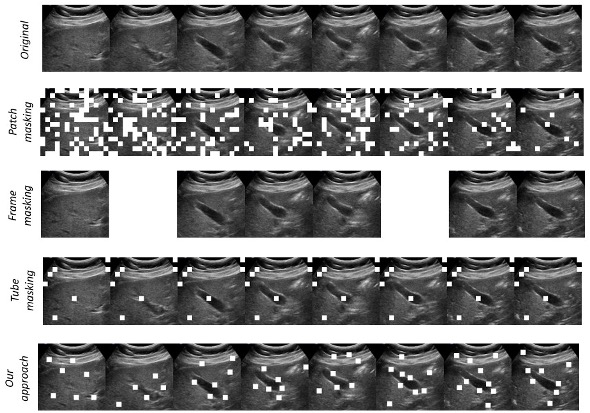
Masked Autoencoders (MAEs). Recently, MAEs [14, 46, 4, 28, 49] have emerged as a promising representation learning technique for vision-related tasks. The idea behind MAE is to mask certain parts (also called tokens) of the input and then try to reconstruct the masked parts from the visible parts as a pretraining task. Usually, a Vision Transformer (ViT) [13] generates the embedding of the tokens. Mask sampling strategy plays a significant role in effectively learning using MAEs [46, 14]. Currently, a random masking strategy is adopted in most MAE approaches [46, 49, 14]. For random masking in videos, patch masking [14], frame masking [51, 38], or tube-based masking (dropping tokens at the same spatial location across a few consecutive frames) [46] are popularly used. Tube-based masking strategy is considered to be better at preventing information leakage arising from redundancy in the time dimension. However, studies suggest that a single masking strategy may not fit all datasets due to the diversity of scenes, acquisition conditions, and high/ low spatiotemporal information regions in videos [4]. For example, Video-MAE [46] achieves the best action classification on the SSv2 dataset [16] with random tube masking. For Kinetics-400, MAE-ST attains the best performance through random patch masking. Fig. 1(a) shows examples of different masking strategies.

Our Proposal. In US videos, GB and malignant regions typically occupy a tiny portion. Notice that these are high information regions as opposed to non-GB portions of the frames, which are low information regions. Thus, random masking (uniform distribution) is not conducive to learning effective representations of malignancy. Few recent approaches suggest using an adaptive mask sampling strategy for more meaningful semantic representation [4, 28]. MGMAE [28] suggests using object motions to guide the mask sampling. AdaMAE [4] exploits a policy gradient optimization strategy by maximizing the expected token reconstruction error in order to boost the sampling probability of the tokens belonging to the objects. Since the organs are mostly stationary in US videos or CT volumes, the motion-guided strategy is not applicable to our case. On the other hand, our experiments show that AdaMAE does not perform significantly better than VideoMAE. By focusing solely on reconstruction error, the model may underrepresent crucial features or patterns within the data. In contrast, we adopt a simple strategy, FocusMAE, in sampling effective masks in the MAE pipeline. We identify candidate high-information regions, and bias the sampling strategy with these region-priors to sample the masking tokens from these focused candidate regions. By using a stronger masking on the high information regions, and reconstructing these tokens, FocusMAE learns a more refined representation.

Contributions. The key contributions of this work are:

1. We posit that existing SOTA techniques for GBC detection in US images exhibit suboptimal accuracy and generalization performance. Consequently, we advocate for a paradigm shift toward video-based GBC detection for US. Also, the problem of US video-centric detection of GBC with machine learning was not previously attempted in literature. We provide the first solution to the problem and present a strong baseline.

2. Even though video-based GBC classification shows improvement over image-based methods in terms of accuracy, specificity, and sensitivity, we observe that the random masking in MAE presents opportunities for further improvement. Notably, the spatiotemporal regions indicative of malignancy typically constitute a small portion of the video. The random selection of masked tokens introduces redundant background information, necessitating a more systematic approach. To address the issue, we propose a novel design, FocusMAE, to systematically bias the masking token selection from the semantically meaningful candidate regions. As a result, the network is compelled to learn a more refined representation of GB malignancy while reconstructing the masked tokens. We report an accuracy of 96.4% using our approach as against 84% by the current SOTA of GBCNet [5] and Radformer [6].

3. Our idea of focused masking is generic, and we validate the generality of the method by applying it to a public CT-based Covid identification task [1]. We report an accuracy gain of 2.2% by our method over the SOTA [47].

4. Concurrently, we curate the most extensive US video dataset available for GBC detection. We establish the dataset by adding 27 US video samples exhibiting GBC to the publicly available GBUSV dataset. The dataset will be made available to the community.

2 Related Work

Deep Learning for GB related Diseases. Several studies have leveraged DNNs to detect various GB conditions, including calculi, cholecystitis, and polyps, using diagnostic images. For instance, [35] applied YOLOv3 to identify the GB and stones in CT images. [11] focused on GB segmentation and employed an AdaBoost classifier for polyp diagnosis. Meanwhile, [30] concentrated on classifying neoplastic polyps in cropped gallbladder ultrasound (USG) images, utilizing an InceptionV3 model. [29] employed ResNet50 to diagnose polypoidal lesions through endoscopic US.

DNNs for GBC Detection. Despite numerous studies on DNNs for gallbladder-related diseases, only a few have explored AI-based detection of GBC [19]. Chang et. al[10] employed a UNet-based denoising to enhance the image quality of Low-Dose CT scans for characterizing GBC. In contrast, Basu et. al[5] introduced a CNN architecture called MS-SoP and a Gaussian blurring-based curriculum for efficient GBC detection in US images. Gupta et. al[20] further studied the performance of MS-SoP in classifying different sub-types of GBC on a large prospective patient cohort. Basu et. al[8] later utilized unsupervised contrastive learning to learn malignancy representations. On the other hand, [6] exploits a transformer-based dual-branch architecture for accurate and explainable GBC detection. [21] investigates application of transformers for differentiation of GBC with xanthogranulomatous cholecystitis. [7] further proposes DETR-based weakly supervised GBC detection. Gupta et. al[18] proposes a calibration metric and loss to calibrate the GBC detection models on small dataset. Despite the above studies, we observe a notable gap in the literature regarding models for video-based GBC detection from US videos. This gap in research motivates the current work.

Video-based Classification and Recognition. Transformers have seen an influx over CNNs due to their superior performance. Transformers with combined spatiotemporal attention [3], hierarchical spatiotemporal attention [34], and separable spatial and temporal attention [33, 9] are popular for video-based recognition or classification.

Masked Autoencoder for Videos. MAEs have gained popularity for self-supervised video representation learning (SSL). [14, 46] extend the MAE from image to video domain. [15] used a combined image and video-based MAE pipeline. On the other hand, [39] introduced running cell masking to reduce cost. Another study [49] recommended masking decoder tokens as well. [4] recommends an adaptive masking strategy instead of random masking. Some studies look for priors like motion trajectory [28, 37, 43]. [32] recommends using semantic parts guided MAE. [17] introduces the usage of both spatial and spatiotemporal attention along with variable token masking ratio.

Figure 2: Overview of the proposed FocusMAE pipeline. Our design proposes guiding the masking tokens with the localization of the candidate focus regions containing high-information. The systematic biasing with focused high-information region priors helps to build a more meaningful reconstruction task for disease representation learning.

3 Proposed Method

3.1 Object Priors in MAE

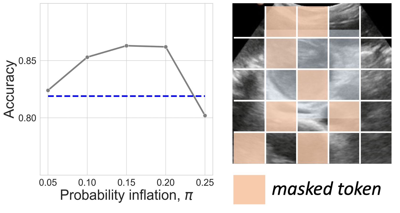
Visual data often demonstrate sparser semantically meaningful information distribution dominated by the foreground objects. Current MAE techniques predominantly use random masking, which may result in sub-optimal results as the information may not be uniformly distributed. For the US videos, GBC often occupies a very humble portion of the frames. Random masking mostly biases the networks to learn representations of redundant backgrounds containing other organs or abdominal cavities. To alleviate the issue, we advocate exploiting the object location priors with high information density to enhance the representation learning in MAE. We show in Fig. 1(b) the preliminary evidence of potential advantages of boosting the masking token probability with object localization priors. We selected a random validation split containing about 20% of our GB US Video dataset. We used the malignant ROI boxes provided in the dataset to specify object locations. We manually increased the masking probability of patches within the bounding box region for the data samples, and used them for self-supervised pretraining. We varied the probability boosting values, denoted by $\pi$, representing the increased probability for patches within the bounding box compared to those in the background. Our experiment reveals that an increase in the masking probability for patches within the bounding box, as opposed to random masking, leads to a noticeable enhancement in results. However, highly inflating masking probability for patches within the bounding box may compromise the integrity of the pretext task and result in performance degradation. These findings underscore the importance of recognizing that distinct image patches contribute differently to the learning of visual representations. Furthermore, the emphasis on reconstructing foreground objects with a balanced approach is crucial for optimal performance.

3.2 FocusMAE Architecture

Video Sub-sampling. Video data contains temporal redundancy as the consecutive frames see a very high overlap in content. We sub-sample the videos to reduce the temporal redundancy. Assuming a video containing $F$ frames, we first sub-sample $\frac{F}{4}$ frames with a stride of $4$. Although the viewpoint in US frames can change very quickly, in our observation of the data, the changes within the frames at a distance equivalent to a stride of 4 from each other are insignificant. Each frame has a size of $3\times H\times W$, $H$, and $W$ stands for the height and width of the frame having three channels (RGB). We further divide these sub-sampled frames for a video into clips – each clip containing 16 frames. We then randomly sample four clips to use during the pretraining phase. Before passing to the pretraining pipeline, the frames are resized to $224\times 224$.

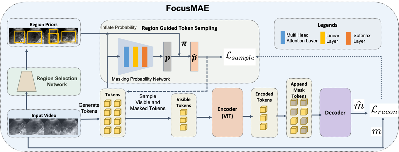
Token Generation. We first divide a video $V$ of size $T\times 3\times H\times W$ into non-overlapping cubic tokens of size $2\times 3\times 16\times 16$. $T$ is the number of frames (temporal dimension), $H$ and $W$ are the height and width of the frames. Each frame has RGB channels. We use a 3D convolution of kernel size = $(2,3,16,16)$, stride $(2,16,16)$, and $d$ output channels. Using this 3d convolution layer, we generate a total of $N=\frac{T}{2}\times\frac{H}{16}\times\frac{W}{16}$ tokens, each of dimension $d$ ($d=384$ in our design) for every video. Next, we add the positional information to the tokens using the fixed 3D periodic positional encoding scheme introduced in [48].

Generating Object Localization Priors. We utilize deep object detection networks as the region proposal network (RPN) to identify the potential GB region within a frame. The predicted bounding boxes are used as potential candidate regions containing the objects (malignancy). We used the public GBCU [5] dataset for training the object detectors. The GBCU dataset provides US images with regions-of-interest marked with bounding boxes. The training focuses on two classes: background and the GB region. We lower the confidence threshold of the predicted boxes to generate multiple candidate regions. These regions are used as priors in a masking token sampler to boost the masking probability of the tokens. If a token’s spatial central point falls within the region prior, then its masking probability is inflated. To define a candidate region for an entire clip, we take the union of the candidate regions for each frame within the clip.

Masked Token Sampling with Region Priors. To generate the masking probabilities for the tokens, we follow [4] and use an auxiliary network consisting of Multi-Head Attention (MHA) with a Linear and a Softmax ($\sigma$) layer following it. Given the embedded tokens $x\in\mathbb{R}^{N\times d}$, the probability scores $p\in\mathbb{R}^{N}$ over all tokens is generated as follows:

$$z=\text{MHA}(x);\quad z\in\mathbb{R}^{N\times d}$$ (1)

$$p=\sigma(\text{Linear}(z));\quad p\in\mathbb{R}^{N}$$ (2)

Region priors then boost the probability score as follows:

$$\hat{p}_{i}=p_{i}+\pi_{i}$$ (3)

If the $i$-th token spatially lies within the candidate regions, then we inflate the masking probability of the token by $\pi_{i}\in(0,\delta)$, where $\delta$ is a small fraction less than $0.25$. We then select without replacement a set of visible token indices $\mathcal{V}\in\{1,\ldots,N\}$ with the probability $(1-\hat{p}_{i})$ for the $i$-th token. The set of masked token indices is given by $\mathcal{M}=\{1,\ldots,N\}\setminus\mathcal{V}$. The number of sampled visible tokens $N_{v}$ is computed based on a pre-defined masking ratio $\rho\in(0,1)$ and equals $(1-\rho)N$.

Encoder. For computational efficiency, only the visible (non-masked) tokens are passed to the encoder. The number of visible tokens is $N_{v}=(1-\rho)N$. We employed a vanilla ViT architecture with space-time attention [9]. The ViT encoder has a depth of 12 layers with 6 heads in each layer. The embedding dimension is 384.

Decoder. The encoded visible tokens are appended with the masked tokens before passing to the decoder. The masked patches are learnable tokens that the decoder learns to reconstruct, guided by the MSE loss between the values of these tokens and their reconstructions. Usually, the decoder in an MAE is a shallow and narrow ViT. However, our experiments indicate that increasing the decoder depth can help in performance gain. We keep the decoder depth to 10 after grid searching for optimal depth. The decoder reconstructs the original video cube of size $\frac{T}{2}\times\frac{H}{16}\times\frac{W}{16}$ from the encoded and masked tokens.

3.3 Training

Masking Reconstruction Loss. We have used the Mean Squared Error loss (MSE) between the predicted and ground-truth RGB values of the masked tokens as the objective function to pretrain the MAE. The loss function is given as:

$$\mathcal{L}_{recon}=\frac{1}{|\mathcal{M}|}\sum_{i\in\mathcal{M}}||\hat{m}_{i}-m_{i}||_{2}$$ (4)

Here $\hat{m}$ and $m$ denote the predicted token and the normalized ground-truth RGB values of the token. $|\mathcal{M}|=\rho N$ refers to the number of masked tokens.

Token Sampling Loss. We use a token sampling loss, $\mathcal{L}_{sample}$, to train the sampling network that generates the sampling probability. We adapt the sampling loss proposed by AdaMAE [4] and use maximization of the average reconstruction error to define the loss. The formulation of such a formulation is motivated by the expected reward maximization of the REINFORCE algorithm in RL. Here, the visible token sampling process is the action, the MAE is the environment, and the masked token reconstruction error is the return. The reconstruction error is high in the high information regions as compared to the low information background regions. Thus, maximizing the expected reconstruction error would result in the network predicting a higher probability score for a high information region. The loss formulation is as follows:

$$\mathcal{L}_{sample}=-\sum_{i\in\mathcal{M}}\big{(}\log{\hat{p}_{i}}\cdot||\hat{m}_{i}-m_{i}||_{2}\big{)}$$ (5)

One key difference with the loss in AdaMAE is that the token probability in our formulation is augmented by the region priors, while AdaMAE uses a token probability for a distribution over the entire image. Thus, we obtain a more refined version of the adaptive token sampling. The log probability tackles the underflow and floating point errors. The gradient flow in the sampling network is kept independent from the ViT encoder and decoder of the main MAE.

Group	Method	Backbone	Acc.	Spec.	Sens.
Human Experts	Radiologist A	–	0.786$\pm$0.134	1.000$\pm$0.000	0.672$\pm$0.201
	Radiologist B	–	0.874$\pm$0.088	1.000$\pm$0.000	0.811$\pm$0.126
Image-based	ResNet50 [25]	CNN	0.711$\pm$0.091	0.822$\pm$0.102	0.672$\pm$0.147
	InceptionV3 [44]	CNN	0.734$\pm$0.089	0.953$\pm$0.072	0.647$\pm$0.107
	Faster-RCNN [41]	CNN	0.757$\pm$0.058	0.687$\pm$0.056	0.808$\pm$0.091
	EfficientDet [45]	CNN	0.789$\pm$0.084	0.761$\pm$0.099	0.828$\pm$0.061
	ViT [13]	Transformer	0.796$\pm$0.068	0.751$\pm$0.128	0.820$\pm$0.076
	DEIT [47]	Transformer	0.829$\pm$0.034	0.787$\pm$0.154	0.845$\pm$0.058
	PVTv2 [50]	Transformer	0.831$\pm$0.041	0.857$\pm$0.167	0.834$\pm$0.068
	GBCNet [5]	CNN	0.840$\pm$0.105	0.843$\pm$0.204	0.843$\pm$0.072
	US-UCL [8]	CNN	0.808$\pm$0.127	0.871$\pm$0.217	0.776$\pm$0.109
	RadFormer (SOTA) [6]	Transformer	0.840$\pm$0.105	0.776$\pm$0.162	0.877$\pm$0.088
Video-based	Video-Swin [34]	Transformer	0.925$\pm$0.053	1.000$\pm$0.000	0.903$\pm$0.085
	TimeSformer [9]	Transformer	0.920$\pm$0.058	0.967$\pm$0.067	0.909$\pm$0.058
	VidTr [33]	Transformer	0.924$\pm$0.038	1.000$\pm$0.000	0.800$\pm$0.072
	VideoMAEv2 [49]	Transformer	0.942$\pm$0.066	0.937$\pm$0.078	0.940$\pm$0.120
	AdaMAE [4]	Transformer	0.947$\pm$0.053	0.952$\pm$0.066	0.913$\pm$0.116
	FocusMAE (Ours)	Transformer	0.964$\pm$0.047	0.910$\pm$0.117	1.000$\pm$0.000

Table 1: The 5-fold cross-validation (Mean$\pm$SD) accuracy, specificity, and sensitivity of baselines and FocusMAE in detecting GBC from the US. FocusMAE achieves the best accuracy and perfect sensitivity, which is much desired for GBC detection. We also report how the expert radiologists perform in detecting GBC from the video dataset. The radiologists were blinded from accessing any patient-related data or clinical/ histopathological findings. The radiologists classified each video using the Gallbladder Reporting and Data Standard (GB-RADS) [22]. Our model outperforms human radiologists in detecting GBC from US videos. Recall that our ground truth labels are biopsy-proven. The performance of the expert radiologists in our study is comparable to literature [20].

Figure 3: Sample video sequences from our US video dataset used for GBC detection, and the public COVID-CT-MD dataset [1]. We show samples of both malignant and benign (non-malignant) sequences for GBC data. For the covid data, we show sample sequences for both Covid and non-Covid categories.

4 Dataset

4.1 Curated US Video Dataset for GBC Detection

Video Data Collection and Curation. We utilized both the public Gallbladder US video dataset (GBUSV) [8] and an additional set of US videos collected by our team of radiologists. The GBUSV dataset comprises 64 Gallbladder US videos, with 32 labeled as benign and another 32 labeled as malignant. To augment our dataset for the video-based gbc detection task, we incorporated 27 additional US videos specifically depicting Gallbladder malignancy.

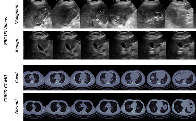
We obtained video samples from patients referred to PGIMER, Chandigarh for abdominal US examinations targeting suspected Gallbladder pathologies. Each patient provided informed written consent during recruitment, and we ensure patient privacy by fully anonymizing the data . Patients were fasting for a minimum of 6 hours to ensure adequate distention of the gb. Our team of radiologists employed a 1-5 MHz curved array transducer (C-1-5D, Logiq S8, GE Healthcare) for the scanning process. The scanning protocol covers the entire gallbladder (including fundus, body, and neck) and any associated lesions or pathologies. We cropped the video frames from the center to safeguard patient privacy and annotations. The processed frames have a size of 360x480 pixels. Fig. 3 shows sample sequences from the dataset.

Annotation. The video labels in GBUSV are already provided. For our additional videos, we relied on the biopsy reports for labeling. Additionally, two radiologists with 2 and 10 years of expertise in abdominal ultrasound (US), were consulted to draw bounding boxes covering the entire GB and the adjacent liver parenchyma in one frame in each video.

Dataset Statistics. The dataset comprises 59 malignant and 32 non-malignant videos, collected from 41 malignant and 32 benign patients, respectively. In total, the dataset encompasses 21,955 frames, with 18,406 frames attributed to videos labeled as malignant.

Dataset Splits. We report the 5-fold cross-validation metrics over the complete dataset for key experiments. The cross-validation splits were conducted on a patient-wise basis, ensuring that all videos of a particular patient appeared exclusively in either the training or the validation split during cross-validation.

4.2 Public CT Dataset for Covid Detection

We use the publicly available COVID-CT-MD dataset [1] to assess the generality of our proposed method across different modalities and diseases. The COVID-CT-MD dataset contains lung CT scans of 169 (108 male and 61 female) confirmed positive COVID-19 cases, 76 (40 male and 36 female) normal cases and 60 (35 male and 25 female) Community-Acquired Pneumonia cases. All samples are annotated at the patient, lobe, and slice levels by three different radiologists. The authors used a Siemens SOMATOM Scope scanner to obtain the scans with the output size of the reconstructed images set to $512\times 512$ pixels. Additionally, the dataset also contains clinical data, including the patient’s age, gender, weight, symptoms, surgery history, follow-up and RT-PCR test reports. However, during our experiments, we did not use the clinical data. We used a stratified random 80:20 split to get the training and validation data.

5 Implementation and Evaluation

Pretraining. We implemented our experiments using PyTorch [36]. We used Kinetics-400 pretrained weights for MAE weight initialization. Although there is a domain gap in natural and medical image data, studies show that pretraining on natural image data improves network performance on medical imaging tasks [2, 12]. We used the video sub-sampling scheme discussed in Sec. 3.2. We apply random-resize cropping, random horizontal flipping, and random scaling as part of the data augmentations for pretraining. We chose ViT-S as the backbone. We use patch size of $2\times 3\times 16\times 16$, resulting in $\frac{16}{2}\times\frac{3}{3}\times\frac{224}{16}\times\frac{224}{16}=1568$ tokens for an input video of size $16\times 3\times 224\times 224$. The pretraining phase is trained with an AdamW optimizer with LR $0.0001$, layer decay $0.75$, and weight decay $0.05$, for minimizing the MSE loss over 300 epochs. The batch size was 2. Warm-up was done for 3 epochs with LR $0.001$.

Fine-tuning. For sub-sampling the videos during fine-tuning, a denser sample rate of 3 was used. We used 16 frames to constitute a clip. From each video, we sampled 5 clips uniformly. During inference, we predict the labels for each of the clips. If any of the clips is predicted as malignant, the entire video is labelled as malignant. We minimized a soft-target cross entropy loss using an AdamW optimizer with LR $1e-5$, layer decay $0.75$, and weight decay $0.05$ for 30 epochs. We used a batch size of 4.

We have used a machine with an Intel Xeon Gold 5218@2.30GHz dual-core processor and 8 Nvidia Tesla V100 32GB GPUs for our experiments.

Evaluation Metrics. We used video-level accuracy, specificity (true negative rate), and sensitivity (true positive rate/ recall) for assessing the video-based GBC identification.

Group	Method	Acc.	Spec.	Sens.
Image-based	ResNet50 [25]	0.721	0.739	0.711
	InceptionV3 [44]	0.672	0.739	0.632
	ViT [13]	0.770	0.783	0.763
	DEIT [47]	0.770	0.696	0.816
Video-based	TimeSformer [9]	0.700	0.739	0.474
	VideoMAE [49]	0.852	0.956	0.789
	FocusMAE (Ours)	0.885	0.895	0.869

Table 2: The performance comparison in terms of accuracy, specificity, and sensitivity of baselines and FocusMAE for detecting COVID from CT [1]. CT-slices are analogous to the video frames, and thus, video-based detection methods are applicable to CT modality as well. Our proposed method consistently outperforms the SOTA baselines on the COVID detection task, establishing the generality and applicability of our method across two different medical imaging modalities – US and CT.

Figure 4: Visual demonstration of the benefit of using the FocusMAE method. (a) Original frames from a US video sequence exhibiting GB malignancy. ROI is drawn in red. (b) Candidate regions as prior (in yellow). (c) Masking by FocusMAE. (d), (e) Attention visualization for the downstream malignancy detection for VideoMAE and FocusMAE, respectively. For FocusMAE, the attention is well guided to the key regions containing the malignancy, as opposed to VideoMAE. (f) CT Slices of a sample Covid patient. (g) Attention visualization of FocusMAE.

6 Experiments and Results

6.1 Efficacy of FocusMAE over SOTA Baselines

We explore the GBC classification performance on US videos for five SOTA video classification methods, namely Video-Swin [34], TimeSformer [9], VidTr [33], VideoMAEv2 [49], and AdaMAE [4].

In addition, we have also explored three SOTA techniques [5, 8, 6] that are specialized for GBC detection on US images. Apart from these specialized models, we analyze the performances of popular image-centric CNN-based classifiers [25, 44] and detectors [41, 45]. We also look into three popular Transformer-based classifiers – ViT [13], DEiT [47], and PvT [50] for GBC detection.

Using Image-based Methods for Video Classification. We use the same video sub-sampling scheme used during the fine-tuning phase (ref. Sec. 5) of the FocusMAE to get the frames and clips. We then use the image-centric methods to predict the labels for each frame in the clips. If the majority of the frames in a clip are predicted as malignant, then the clip is predicted as malignant. If any clip within a video is predicted as malignant, the overall video is categorized as malignant. The image-based methods were pretrained on the public GBCU [5] dataset.

Quantitative Analysis. We show the 5-fold cross-validation performance in terms of accuracy, specificity, and sensitivity for the baselines and the proposed FocusMAE in Tab. 1. Clearly, the video-based techniques trump the image-centric SOTA methods of GBC detection, supporting our recommendation of a paradigm shift to video-based classification for the problem. Additionally, we see the effectiveness of the FocusMAE in detecting GBC.

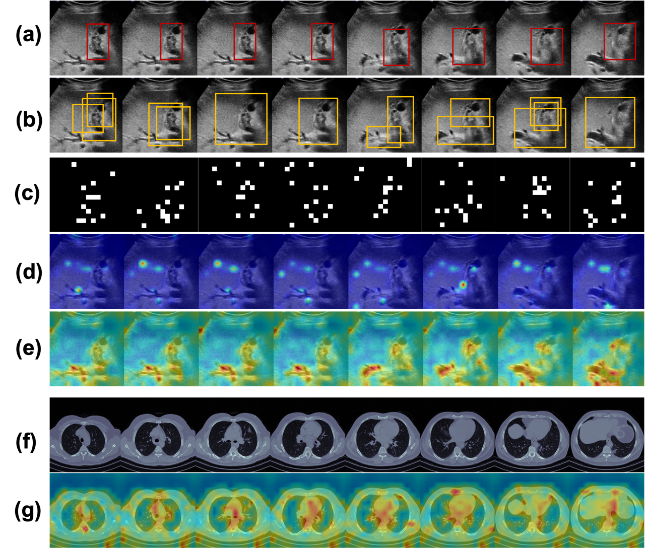
Qualitative Analysis. We show the qualitative analysis in Fig. 4. The random masking by VideoMAE does not adequately mask the high-information malignant region. In contrast, the region prior guided FocusMAE generates stronger masking for learning the malignant representation by biasing the masking towards the malignancy localization region. We visualize the attention rollout during the downstream task. Clearly, FocusMAE’s attention regions highlight semantically more meaningful areas, such as the gallbladder boundary and anatomical structures, compared to VideoMAE.

6.2 Generality of the Proposed Method

We explored the generality of the proposed FocusMAE method on the task of Covid detection from a publicly available CT dataset [1]. Tab. 2 shows that FocusMAE achieves much better accuracy, specificity, and sensitivity, indicating the superiority of the disease representation learning capability of FocusMAE. The applicability of FocusMAE on two distinct tasks - 1) GBC detection from US videos, and 2) Covid detection from CT - establishes the generality of the method across two diagnostic modalities, and diseases.

(a)

(b)

(c)

(d)

Figure 5: Ablation study. We report the mean scores over 5-fold cross-validation for GBC detection. (a) Effect of varying the masking ratio ($\rho$) on accuracy. (b) Effect of varying the reconstruction loss - L1 vs. MSE - for SSL pretraining. Training with MSE yields 2.1% better accuracy. (c) Performance for different backbones. (d) Effect of varying the decoder depth.

Figure 6: Visuals of candidate regions. Red – malignant regions identified by radiologists. Yellow – candidate object localization generated by the RPN.

6.3 Ablation Study

We performed the ablation study on the FocusMAE with the ViT backbone on the US Video dataset.

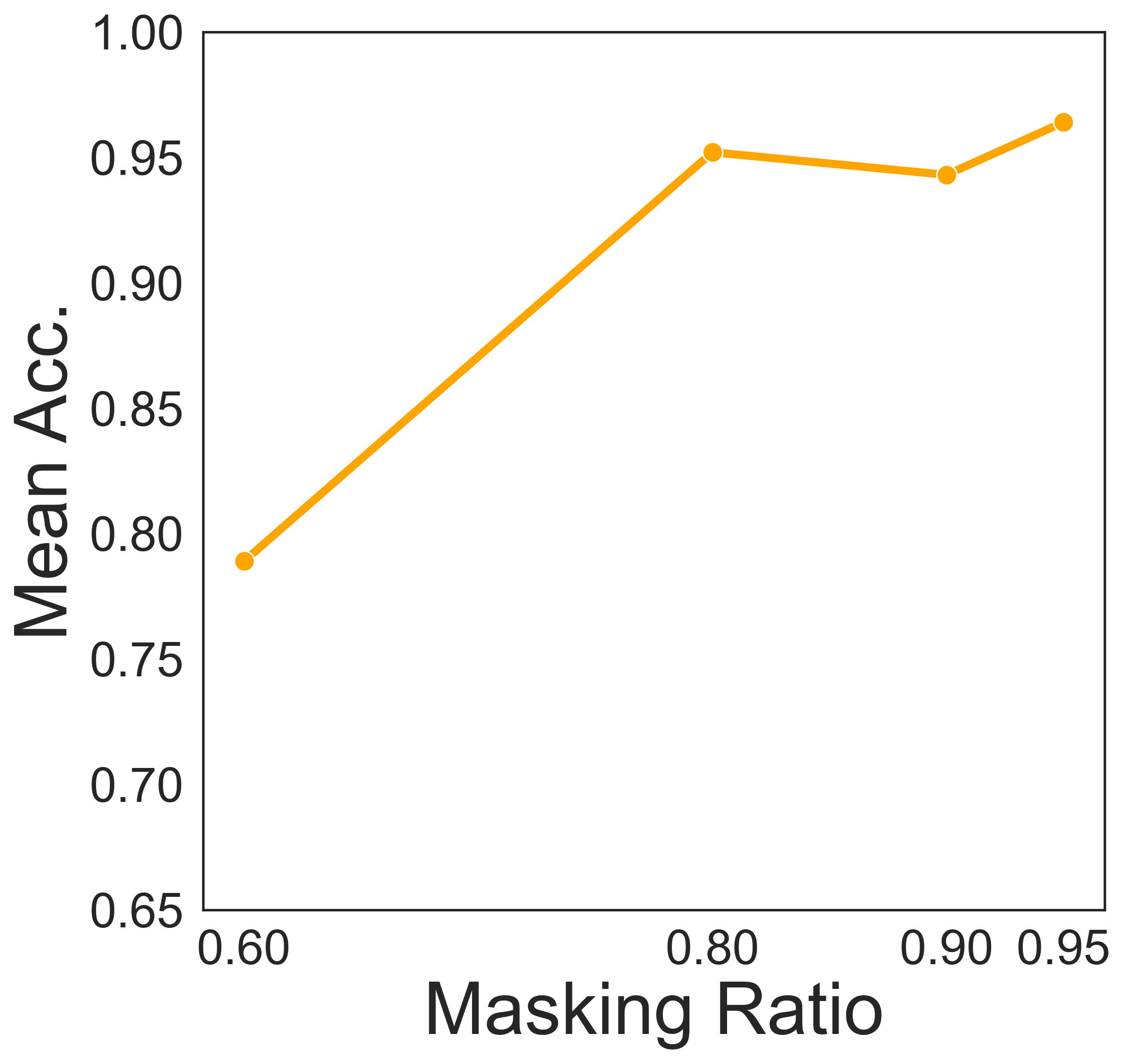
Masking Ratio. Fig. 5(a) shows how the masking ratio $\rho$ influences the performance of FocusMAE. For FocusMAE, 95% masking ratio achieves the best accuracy of 96.4%. VideoMAE uses a 90% masking ratio with random tube-based masking. The region-prior guided approach helps FocusMAE to sample more informative tokens with lower redundancy than VideoMAE.

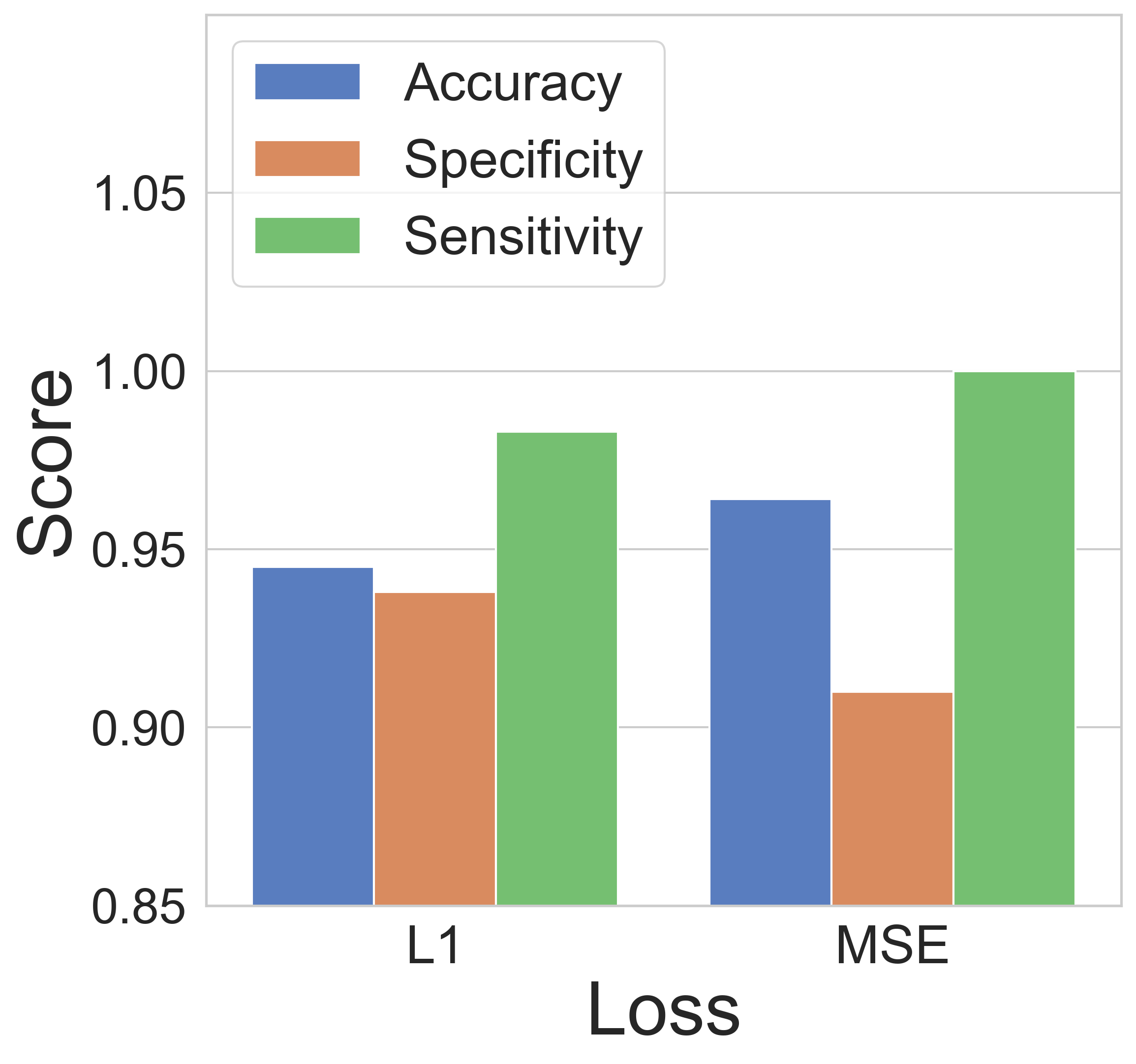
Reconstruction Loss. We examined the effect of varying the reconstruction loss function in our study. We experimented with two variants: Mean Absolute Error or L1-loss, and Mean Squared Error (MSE). The results, shown in Fig. 5(b), indicate that using MSE loss during pretraining produces slightly better performance in terms of accuracy. Models trained with MSE loss demonstrated 2.1% higher mean accuracy compared to those trained with L1 loss.

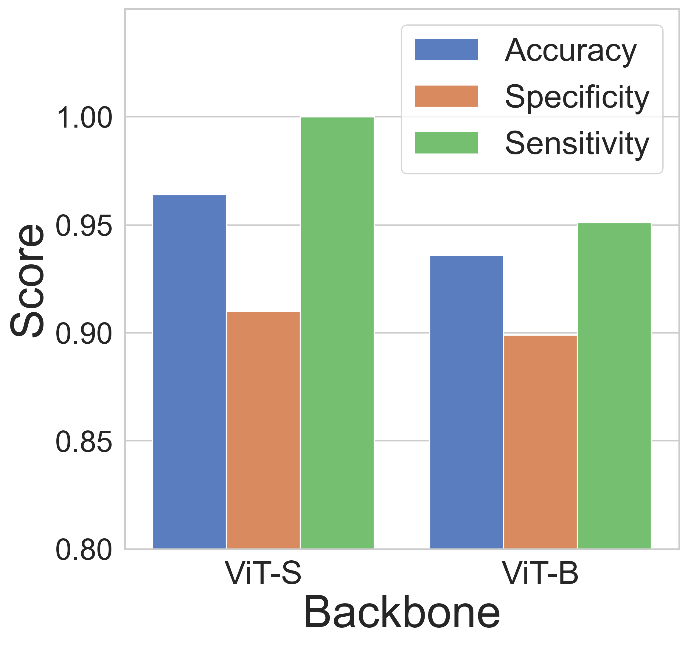
Encoder Backbone. Fig. 5(c) demonstrates the effect of ViT variants on the token encoding task. We experimented with ViT-S and ViT-B. We observe that larger backbones do not perform well for our data, indicating potential over-fitting.

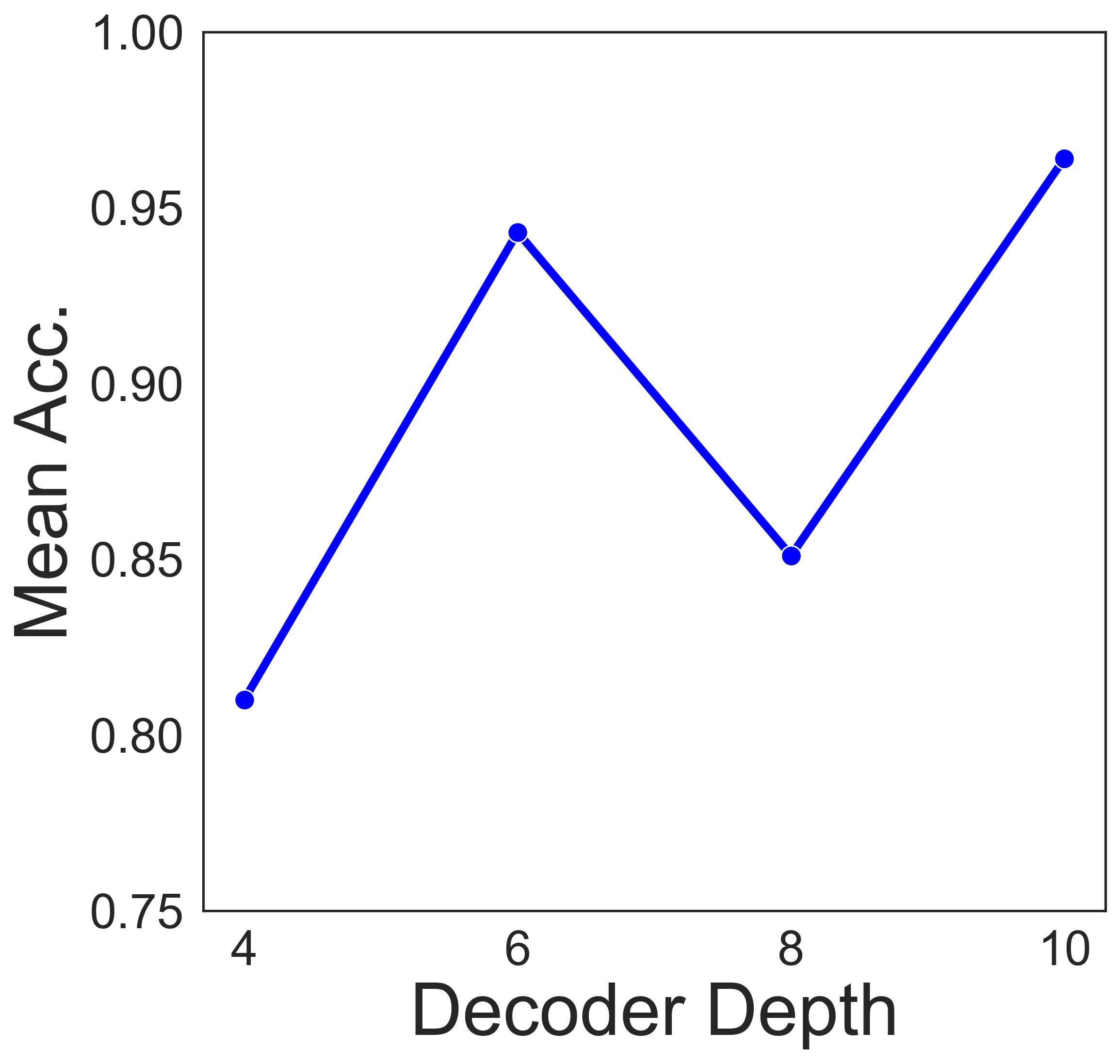
Decoder Depth. We experiment with the number of decoder blocks and present the result in Fig. 5(d). We see performance gain when the decoder depth is varied from 4 to 6. However, there is a drop in performance when the decoder depth is increased to 8. The observation is consistent with [46, 4]. Interestingly, when we increased the depth further, we saw an increase in accuracy, which indicates that the decoder can benefit from increasing the depth and need not necessarily be a shallow network.

6.4 Analysis on Candidate Region Selection

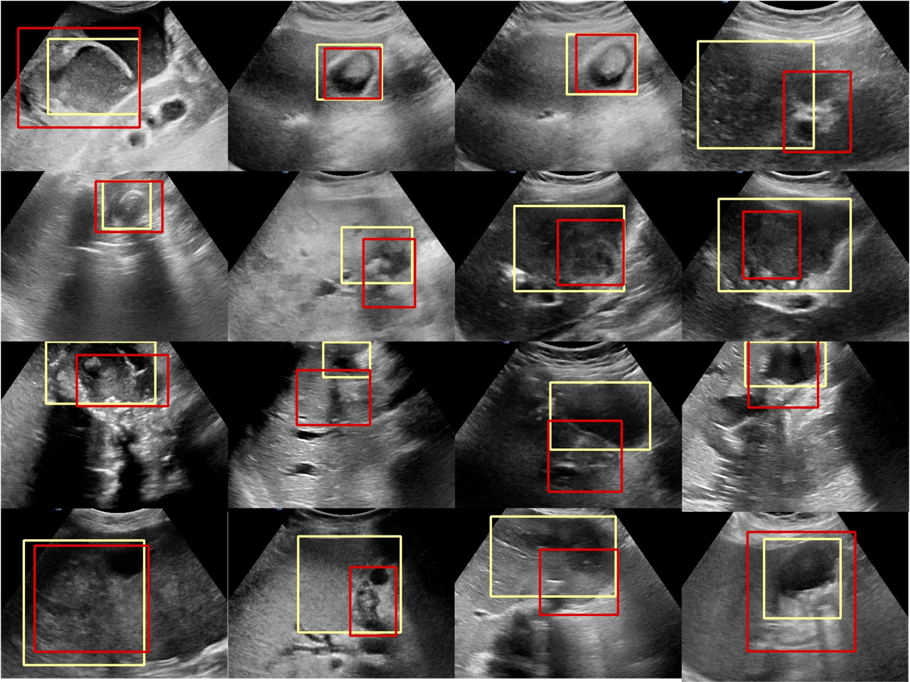
Fig. 6 shows sample object region localization of the RPN. We adopted a FasterRCNN-based RPN for generating the candidate regions for using as priors in FocusMAE. The RPN achieves mIoU of 0.712 with a recall rate of 0.994.

7 Conclusion

This study addresses the limitations of current US image-based GBC detection techniques, emphasizing the need for a paradigm shift towards US video-based approaches. Our novel design, named FocusMAE, strategically biases masking token selection from high-information regions and learns quality representations of GB malignancy. FocusMAE achieves state-of-the-art results on US video-based GBC detection. We hope that our work will spark interest in the challenging problem of GBC detection from US videos. Moreover, we showcase the generality of FocusMAE by applying it successfully to a public lung CT-based Covid detection task, demonstrating its applicability across two modalities and diseases. This suggests that FocusMAE could find broader use-cases in future, marking it a promising step towards versatile diagnostic solutions.

Acknowledgments. Authors thank Dr. Shravya Singh and Dr. Ruby Siddiqui for data annotation, and Dr. Pratyaksha Rana for reading the cases. This work was partially supported by the CSE Research Acceleration Fund of IIT Delhi.

Supplementary Material

Appendix A Region Selection Network

We have experimented with multiple deep detectors to localize the candidate regions. We haven’t used the bounding box annotations in the video for training the candidate region networks. Instead, we used the public GBCU dataset to pretrain the detectors for localizing the malignancy. We then lowered the threshold to generate multiple candidate regions for the video frames used in the FocusMAE experiments.

To calculate precision and recall in the GB localization phase, following the recommendation of [42], we determine a predicted region as a true positive if its center falls within the bounding box of the ground truth region. Conversely, if the center is outside the bounding box, we categorize the prediction as a false positive attributed to localization error. Tab. S1 shows the mIoU and the recall for the different candidate region detectors.

Fig. S1 shows sample object region localization of the RPN. We adopted a FasterRCNN-based RPN for generating the candidate regions for using as priors in FocusMAE as the detector achieves the best recall rate.

Model	mIoU	Precision	Recall
Faster-RCNN	0.712	0.952	0.994
YOLO	0.767	0.979	0.962
CentripetalNet	0.614	0.947	0.909
Reppoints	0.682	0.942	0.997
DETR	0.724	0.962	0.988

Table S1: Comparison of the candidate region selection models.

Figure S1: Sample candidate bounding boxes generated by the region selection network.

Appendix B Region Selection Network Implementation

We adopted the Faster-RCNN [41] model for candidate region selection. A frozen Resnet50 Feature Pyramid backbone is used. The input size was $800\times 1333\times 3$. We used a SGD optimizer with LR = 0.005, momentum = 0.9, and weight decay = 0.0005. We used a batch size of 16 and trained for 60 epochs on the GBCU dataset.

Appendix C Visualization

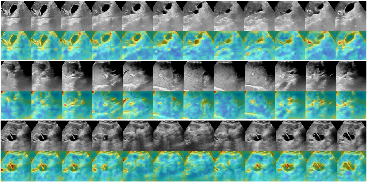
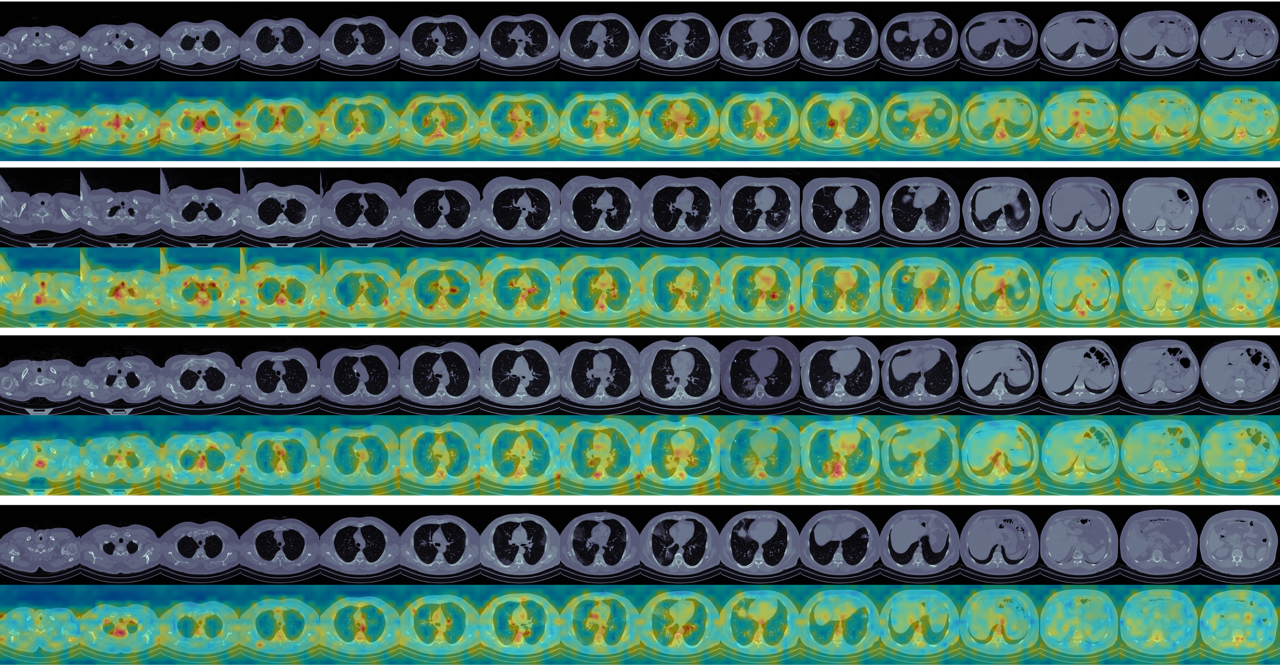
Fig. S2 and Fig. S3 show the attention visuals for the proposed FocusMAE method on additional data samples. Evidently, FocusMAE is able to attend the salient regions for disease detection.

Figure S2: Attention visuals for FocusMAE for the GBC detection task on the US videos. We show three different maligant video samples. For each video sample, the upper row shows the sequence with the original frames, and the lower row shows the attention on the frames.

Figure S3: Attention visuals for FocusMAE for COVID detection from CT images. We show four COVID CT samples. For each sample, the upper row shows the sequence with the original CT slices, and the lower row shows the attention on these slices.

Model	Description	Input Size	Optimizer	Batch size	Epochs/ Steps
VideoMAEv2 [49]	Vision transformer (ViT) backbone, with random masked auto-encoders. Masking in both encoder and decoders. All attention-based layers were trainable. ViT base model used for inference.	$3\times 16\times 224\times 224$	AdamW, LR = 7e-5, momentum = 0.999 ,weight decay = 0.1	4	30 epochs
TimeSformer [9]	Vision transformer based space time atention. Divided space-time attention configuration used. ViT base model used for inference.	$3\times 8\times 224\times 224$	SGD, LR = 0.005, weight decay=1e-4, momentum=0.9	8	25 epochs
VideoSwin [34]	Pretrained on ImageNet-1K. SwinTransformer3D based backbone. All layers were trainable	$3\times 8\times 224\times 224$	SGD, LR = 0.01, weight decay=1e-4, momentum=0.9	4	30 epochs
AdaMAE [4]	Vision transformer (ViT) backbone, with adaptively masked auto-encoders. The model embedding size provided by the authors is 768; we have pre-trained the 384 version to allow for a better fit to our data. Masking in only encoders. All attention-based layers were trainable. ViT base model used for inference	$3\times 16\times 224\times 224$	AdamW, LR = 1e-6, weight decay=0.9, momentum=0.99	2	10 epochs
VidTr [33]	Transformer-based video classification with separable attention. ViT-B backbone. All layers were trainable.	$3\times 16\times 224\times 224$	SGD, LR = 3e-4, weight decay=1e-5, momentum=0.9	2	40 epochs

Table S2: Implementation details for the different video-based baseline networks used for US video-based classification of Gallbladder Cancer. All details are for finetuning on the GB US video dataset. Pretraining details for VideoMAE and AdaMAE are already discussed.

Appendix D Baseline Implementation Details

Tab. S2 lists the configurations of all baseline models used in this study. We trained our models on 4 Nvidia Tesla V100 32GB GPUs. The table includes a brief description of the model, input sizes, optimizer parameters, other relevant hyper-parameters such as learning rate, weight decay, momentum, batch size, and the number of training epochs for the network.

For VideoMAEv2 pretraining, we used a Vision transformer (ViT) backbone, with random masked auto-encoders. Masking was done in both encoder and decoders. All attention-based layers were trainable. We used the ViT-S model. The input size was $3\times 16\times 224\times 224$. We initiated the ViT weights with the Kinetics-pretrained VideoMAE weights. We have optimized the MSE loss for original and reconstructed masked patches on the GBC US Video dataset using an AdamW optimizer with LR = 1e-4 and momentum = 0.95. We used a batch size of 32 and trained for 1200 epochs.

AdaMAE pretraining was an adoption of the VideoMAE pretraining procedure. We used the ViT-S backbone, with adaptively masked auto-encoders. We have pre-trained the model with embedding dimension 384 to allow for a better fit to our data. We have used masking in only encoders. All attention-based layers were trainable. Similar to VideoMAE, we initialized the weights with the Kinetics preained AdaMAE weights. We used the MSE loss and used an AdamW optimizer with LR = 1e-4 and momentum = 0.95. The input sizes are $3\times 16\times 224\times 224$. We used batch size of 8 and pretrained for 500 epochs.

Appendix E Clip-level Statistics

We have a total of 484 clips sub-sampled from the 91 videos at the fine-tuning stage. Out of these, 320 clips were from the malignant videos, and contain the malignant label as per the positive biopsy reports. All clips of a malignant video is given the malignant label. Radiologists identified 199 clips out of these 320 to be malignant. At a frame-level, radiologists identified 3212 frames exhibiting signs of malignancy.

References

- [1] Parnian Afshar, Shahin Heidarian, Nastaran Enshaei, Farnoosh Naderkhani, Moezedin Javad Rafiee, Anastasia Oikonomou, Faranak Babaki Fard, Kaveh Samimi, Konstantinos N Plataniotis, and Arash Mohammadi. Covid-ct-md, covid-19 computed tomography scan dataset applicable in machine learning and deep learning. Scientific Data, 8(1):121, 2021.
- [2] Laith Alzubaidi, Mohammed A Fadhel, Omran Al-Shamma, Jinglan Zhang, J Santamaría, Ye Duan, and Sameer R Oleiwi. Towards a better understanding of transfer learning for medical imaging: a case study. Applied Sciences, 10(13):4523, 2020.
- [3] Anurag Arnab, Mostafa Dehghani, Georg Heigold, Chen Sun, Mario Lučić, and Cordelia Schmid. Vivit: A video vision transformer. In Proceedings of the IEEE/CVF international conference on computer vision, pages 6836–6846, 2021.
- [4] Wele Gedara Chaminda Bandara, Naman Patel, Ali Gholami, Mehdi Nikkhah, Motilal Agrawal, and Vishal M Patel. Adamae: Adaptive masking for efficient spatiotemporal learning with masked autoencoders. In Proceedings of the IEEE/CVF Conference on Computer Vision and Pattern Recognition, pages 14507–14517, 2023.
- [5] Soumen Basu, Mayank Gupta, Pratyaksha Rana, Pankaj Gupta, and Chetan Arora. Surpassing the human accuracy: Detecting gallbladder cancer from usg images with curriculum learning. In CVPR, pages 20886–20896, 2022.
- [6] Soumen Basu, Mayank Gupta, Pratyaksha Rana, Pankaj Gupta, and Chetan Arora. Radformer: Transformers with global–local attention for interpretable and accurate gallbladder cancer detection. Medical Image Analysis, 83:102676, 2023.
- [7] Soumen Basu, Ashish Papanai, Mayank Gupta, Pankaj Gupta, and Chetan Arora. Gall bladder cancer detection from us images with only image level labels. In International Conference on Medical Image Computing and Computer-Assisted Intervention, pages 206–215. Springer, 2023.
- [8] Soumen Basu, Somanshu Singla, Mayank Gupta, Pratyaksha Rana, Pankaj Gupta, and Chetan Arora. Unsupervised contrastive learning of image representations from ultrasound videos with hard negative mining. In MICCAI, pages 423–433. Springer, 2022.
- [9] Gedas Bertasius, Heng Wang, and Lorenzo Torresani. Is space-time attention all you need for video understanding? In ICML, volume 2, page 4, 2021.
- [10] Yigang Chang, Qian Wu, Limin Chi, and Huaying Huo. Ct manifestations of gallbladder carcinoma based on neural network. Neural Computing and Applications, pages 1–6, 2022.
- [11] Tao Chen, Shaoxiong Tu, Haolu Wang, Xuesong Liu, Fenghua Li, Wang Jin, Xiaowen Liang, Xiaoqun Zhang, and Jian Wang. Computer-aided diagnosis of gallbladder polyps based on high resolution ultrasonography. Computer methods and programs in biomedicine, 185:105118, 2020.
- [12] Phillip M Cheng and Harshawn S Malhi. Transfer learning with convolutional neural networks for classification of abdominal ultrasound images. Journal of digital imaging, 30(2):234–243, 2017.
- [13] Alexey Dosovitskiy, Lucas Beyer, Alexander Kolesnikov, Dirk Weissenborn, Xiaohua Zhai, Thomas Unterthiner, Mostafa Dehghani, Matthias Minderer, Georg Heigold, Sylvain Gelly, et al. An image is worth 16x16 words: Transformers for image recognition at scale. arXiv preprint arXiv:2010.11929, 2020.
- [14] Christoph Feichtenhofer, Yanghao Li, Kaiming He, et al. Masked autoencoders as spatiotemporal learners. Advances in neural information processing systems, 35:35946–35958, 2022.
- [15] Rohit Girdhar, Alaaeldin El-Nouby, Mannat Singh, Kalyan Vasudev Alwala, Armand Joulin, and Ishan Misra. Omnimae: Single model masked pretraining on images and videos. In Proceedings of the IEEE/CVF Conference on Computer Vision and Pattern Recognition, pages 10406–10417, 2023.
- [16] Raghav Goyal, Samira Ebrahimi Kahou, Vincent Michalski, Joanna Materzynska, Susanne Westphal, Heuna Kim, Valentin Haenel, Ingo Fruend, Peter Yianilos, Moritz Mueller-Freitag, et al. The” something something” video database for learning and evaluating visual common sense. In Proceedings of the IEEE international conference on computer vision, pages 5842–5850, 2017.
- [17] Agrim Gupta, Stephen Tian, Yunzhi Zhang, Jiajun Wu, Roberto Martín-Martín, and Li Fei-Fei. Maskvit: Masked visual pre-training for video prediction. arXiv preprint arXiv:2206.11894, 2022.
- [18] Mayank Gupta, Soumen Basu, and Chetan Arora. How reliable are the metrics used for assessing reliability in medical imaging? In International Conference on Medical Image Computing and Computer-Assisted Intervention, pages 149–158. Springer, 2023.
- [19] Pankaj Gupta, Soumen Basu, and Chetan Arora. Applications of artificial intelligence in biliary tract cancers. Indian Journal of Gastroenterology, pages 1–12, 2024.
- [20] Pankaj Gupta, Soumen Basu, Pratyaksha Rana, Usha Dutta, Raghuraman Soundararajan, Daneshwari Kalage, Manika Chhabra, Shravya Singh, Thakur Deen Yadav, Vikas Gupta, et al. Deep-learning enabled ultrasound based detection of gallbladder cancer in northern india: a prospective diagnostic study. The Lancet Regional Health-Southeast Asia, 2023.
- [21] Pankaj Gupta, Soumen Basu, Thakur Deen Yadav, Lileswar Kaman, Santosh Irrinki, Harjeet Singh, Gaurav Prakash, Parikshaa Gupta, Ritambhra Nada, Usha Dutta, et al. Deep-learning models for differentiation of xanthogranulomatous cholecystitis and gallbladder cancer on ultrasound. Indian Journal of Gastroenterology, pages 1–8, 2023.
- [22] Pankaj Gupta, Usha Dutta, Pratyaksha Rana, Manphool Singhal, Ajay Gulati, Naveen Kalra, Raghuraman Soundararajan, Daneshwari Kalage, Manika Chhabra, Vishal Sharma, et al. Gallbladder reporting and data system (gb-rads) for risk stratification of gallbladder wall thickening on ultrasonography: an international expert consensus. Abdominal Radiology, pages 1–12, 2021.
- [23] Pankaj Gupta, Yashi Marodia, Akash Bansal, Naveen Kalra, Praveen Kumar-M, Vishal Sharma, Usha Dutta, and Manavjit Singh Sandhu. Imaging-based algorithmic approach to gallbladder wall thickening. World journal of gastroenterology, 26(40):6163, 2020.
- [24] Pankaj Gupta, Kesha Meghashyam, Yashi Marodia, Vikas Gupta, Rajender Basher, Chandan Krushna Das, Thakur Deen Yadav, Santhosh Irrinki, Ritambhra Nada, and Usha Dutta. Locally advanced gallbladder cancer: a review of the criteria and role of imaging. Abdominal Radiology, 46(3):998–1007, 2021.
- [25] Kaiming He, Xiangyu Zhang, Shaoqing Ren, and Jian Sun. Deep residual learning for image recognition. In CVPR, pages 770–778, 2016.
- [26] Eun Kyung Hong, Kun Kuk Kim, Jung Nam Lee, Woon Kee Lee, Min Chung, Yeon Suk Kim, and Yeon Ho Park. Surgical outcome and prognostic factors in patients with gallbladder carcinoma. Annals of Hepato-Biliary-Pancreatic Surgery, 18(4):129–137, 2014.
- [27] NNAM Howlader, AM Noone, M Krapcho, D Miller, K Bishop, CL Kosary, M Yu, J Ruhl, Z Tatalovich, A Mariotto, et al. Seer cancer statistics review, 1975-2014, national cancer institute. Bethesda, MD, pages 1–12, 2017.
- [28] Bingkun Huang, Zhiyu Zhao, Guozhen Zhang, Yu Qiao, and Limin Wang. Mgmae: Motion guided masking for video masked autoencoding. In Proceedings of the IEEE/CVF International Conference on Computer Vision, pages 13493–13504, 2023.
- [29] Sung Ill Jang, Young Jae Kim, Eui Joo Kim, Huapyong Kang, Seung Jin Shon, Yu Jin Seol, Dong Ki Lee, Kwang Gi Kim, and Jae Hee Cho. Diagnostic performance of endoscopic ultrasound-artificial intelligence using deep learning analysis of gallbladder polypoid lesions. Journal of Gastroenterology and Hepatology, 36(12):3548–3555, 2021.
- [30] Younbeom Jeong, Jung Hoon Kim, Hee-Dong Chae, Sae-Jin Park, Jae Seok Bae, Ijin Joo, and Joon Koo Han. Deep learning-based decision support system for the diagnosis of neoplastic gallbladder polyps on ultrasonography: preliminary results. Scientific Reports, 10(1):1–10, 2020.
- [31] Masahiko Kinoshita, Daiju Ueda, Toshimasa Matsumoto, Hiroji Shinkawa, Akira Yamamoto, Masatsugu Shiba, Takuma Okada, Naoki Tani, Shogo Tanaka, Kenjiro Kimura, et al. Deep learning model based on contrast-enhanced computed tomography imaging to predict postoperative early recurrence after the curative resection of a solitary hepatocellular carcinoma. Cancers, 15(7):2140, 2023.
- [32] Gang Li, Heliang Zheng, Daqing Liu, Chaoyue Wang, Bing Su, and Changwen Zheng. Semmae: Semantic-guided masking for learning masked autoencoders. arXiv preprint arXiv:2206.10207, 2022.
- [33] Xinyu Li, Yanyi Zhang, Chunhui Liu, Bing Shuai, Yi Zhu, Biagio Brattoli, Hao Chen, Ivan Marsic, and Joseph Tighe. Vidtr: Video transformer without convolutions. arXiv e-prints, pages arXiv–2104, 2021.
- [34] Ze Liu, Jia Ning, Yue Cao, Yixuan Wei, Zheng Zhang, Stephen Lin, and Han Hu. Video swin transformer. In Proceedings of the IEEE/CVF conference on computer vision and pattern recognition, pages 3202–3211, 2022.
- [35] Shanchen Pang, Tong Ding, Sibo Qiao, Fan Meng, Shuo Wang, Pibao Li, and Xun Wang. A novel yolov3-arch model for identifying cholelithiasis and classifying gallstones on ct images. PloS one, 14(6):e0217647, 2019.
- [36] Adam Paszke, Sam Gross, Francisco Massa, Adam Lerer, James Bradbury, Gregory Chanan, Trevor Killeen, Zeming Lin, Natalia Gimelshein, Luca Antiga, et al. Pytorch: An imperative style, high-performance deep learning library. Advances in neural information processing systems, 32, 2019.
- [37] Mandela Patrick, Dylan Campbell, Yuki Asano, Ishan Misra, Florian Metze, Christoph Feichtenhofer, Andrea Vedaldi, and Joao F Henriques. Keeping your eye on the ball: Trajectory attention in video transformers. Advances in neural information processing systems, 34:12493–12506, 2021.
- [38] Rui Qian, Tianjian Meng, Boqing Gong, Ming-Hsuan Yang, Huisheng Wang, Serge Belongie, and Yin Cui. Spatiotemporal contrastive video representation learning. In Proceedings of the IEEE/CVF Conference on Computer Vision and Pattern Recognition, pages 6964–6974, 2021.
- [39] Zhiwu Qing, Shiwei Zhang, Ziyuan Huang, Xiang Wang, Yuehuan Wang, Yiliang Lv, Changxin Gao, and Nong Sang. Mar: Masked autoencoders for efficient action recognition. IEEE Transactions on Multimedia, 2023.
- [40] Giorgia Randi, Silvia Franceschi, and Carlo La Vecchia. Gallbladder cancer worldwide: geographical distribution and risk factors. International journal of cancer, 118(7):1591–1602, 2006.
- [41] Shaoqing Ren, Kaiming He, Ross Girshick, and Jian Sun. Faster r-cnn: Towards real-time object detection with region proposal networks. In C. Cortes, N. D. Lawrence, D. D. Lee, M. Sugiyama, and R. Garnett, editors, Advances in Neural Information Processing Systems 28, pages 91–99. Curran Associates, Inc., 2015.
- [42] Dezső Ribli, Anna Horváth, Zsuzsa Unger, Péter Pollner, and István Csabai. Detecting and classifying lesions in mammograms with deep learning. Scientific reports, 8(1):1–7, 2018.
- [43] Xinyu Sun, Peihao Chen, Liangwei Chen, Changhao Li, Thomas H. Li, Mingkui Tan, and Chuang Gan. Masked motion encoding for self-supervised video representation learning. In Proceedings of the IEEE/CVF Conference on Computer Vision and Pattern Recognition (CVPR), pages 2235–2245, June 2023.
- [44] Christian Szegedy, Vincent Vanhoucke, Sergey Ioffe, Jon Shlens, and Zbigniew Wojna. Rethinking the inception architecture for computer vision. In Proceedings of the IEEE conference on computer vision and pattern recognition, pages 2818–2826, 2016.
- [45] Mingxing Tan, Ruoming Pang, and Quoc V Le. Efficientdet: Scalable and efficient object detection. In Proc. IEEE CVPR, pages 10781–10790, 2020.
- [46] Zhan Tong, Yibing Song, Jue Wang, and Limin Wang. Videomae: Masked autoencoders are data-efficient learners for self-supervised video pre-training. Advances in neural information processing systems, 35:10078–10093, 2022.
- [47] Hugo Touvron, Matthieu Cord, Matthijs Douze, Francisco Massa, Alexandre Sablayrolles, and Hervé Jégou. Training data-efficient image transformers & distillation through attention. In ICML, pages 10347–10357. PMLR, 2021.
- [48] Ashish Vaswani, Noam Shazeer, Niki Parmar, Jakob Uszkoreit, Llion Jones, Aidan N Gomez, Łukasz Kaiser, and Illia Polosukhin. Attention is all you need. Advances in neural information processing systems, 30, 2017.
- [49] Limin Wang, Bingkun Huang, Zhiyu Zhao, Zhan Tong, Yinan He, Yi Wang, Yali Wang, and Yu Qiao. Videomae v2: Scaling video masked autoencoders with dual masking. In Proceedings of the IEEE/CVF Conference on Computer Vision and Pattern Recognition, pages 14549–14560, 2023.
- [50] Wenhai Wang, Enze Xie, Xiang Li, Deng-Ping Fan, Kaitao Song, Ding Liang, Tong Lu, Ping Luo, and Ling Shao. Pvtv2: Improved baselines with pyramid vision transformer, 2021.
- [51] Chen Wei, Haoqi Fan, Saining Xie, Chao-Yuan Wu, Alan Yuille, and Christoph Feichtenhofer. Masked feature prediction for self-supervised visual pre-training. In Proceedings of the IEEE/CVF Conference on Computer Vision and Pattern Recognition, pages 14668–14678, 2022.