Thermometer: Towards Universal Calibration for Large Language Models

Abstract

We consider the issue of calibration in large language models (LLM). Recent studies have found that common interventions such as instruction tuning often result in poorly calibrated LLMs. Although calibration is well-explored in traditional applications, calibrating LLMs is uniquely challenging. These challenges stem as much from the severe computational requirements of LLMs as from their versatility, which allows them to be applied to diverse tasks. Addressing these challenges, we propose thermometer, a calibration approach tailored to LLMs. thermometer learns an auxiliary model, given data from multiple tasks, for calibrating a LLM. It is computationally efficient, preserves the accuracy of the LLM, and produces better-calibrated responses for new tasks. Extensive empirical evaluations across various benchmarks demonstrate the effectiveness of the proposed method.

1 Introduction

Calibration is a desirable property of any probabilistic forecaster. Well-calibrated forecasts ensure that probabilities produced by the forecaster can be interpreted as accurate confidence estimates of the forecasts. Informally, this implies that the forecaster is more often wrong on predictions made with low probabilities than those made with high probabilities. Well-calibrated forecasts are crucial for both enabling trust in the forecaster’s predictions and incorporating the forecasts as part of a larger autonomous or semi-autonomous system.

Large language models (LLMs) (Brown et al., 2020; Raffel et al., 2020; Touvron et al., 2023) define probability distributions over sequences of tokens and produce probabilistic forecasts over future tokens in a sequence and corresponding semantic entities represented by the tokens. Their ability to synthesize knowledge from large volumes of data, represented as sequences of tokens, has led to remarkable performance on diverse tasks, including question answering (Hendrycks et al., 2021), commonsense reasoning (Zhong et al., 2019), and machine translation (Zhu et al., 2020) among others. However, much like other probabilistic forecasters, before deploying LLMs in critical applications, it is important that they are well-calibrated in addition to being accurate. Unfortunately, a growing body of evidence suggests that while pre-trained LLMs are often well-calibrated, alignment interventions such as instruction tuning which make the pre-trained LLMs more usable, also harm calibration (OpenAI, 2023; Zhu et al., 2023).

While calibration has long been studied (Brier, 1950; Dawid, 1982; Gneiting et al., 2007) and different approaches for improving calibration properties of probabilistic forecasters exist (Platt et al., 1999; Lakshminarayanan et al., 2017; Gal and Ghahramani, 2016; Guo et al., 2017), LLMs pose unique challenges. Training a LLM is expensive, and even inference typically incurs non-negligible expenses. This makes any calibration approach that requires multiple training runs prohibitively expensive. Even approaches that only require multiple inferences at test time can be unreasonably expensive for certain applications. Moreover, owing to their versatility, instruction-tuned LLMs are often applied, without further adaptation, to a diverse array of tasks. It is essential that methods for calibrating them do not affect the accuracy of the uncalibrated LLMs and that the calibration methods themselves can adapt to new tasks. Finally, measuring and alleviating calibration is challenging in cases where the LLM is required to generate free-form text. The equivalence class defined by the LLM-generated sequences that map to the same semantic content is large, making it challenging to assign meaningful confidence to the generation or even robustly assess the quality of the generation.

We present thermometer for calibrating LLMs while alleviating the above challenges. thermometer learns, from multiple tasks, a parameterized mapping to map the outputs of the LLM to better-calibrated probabilities. Our approach is (i) computationally efficient: we do not require multiple training runs, and at inference time, we are only $\sim 0.5\%$ slower than the uncalibrated LLM, (ii) accuracy preserving: we build on temperature scaling (Guo et al., 2017) which ensures that the predictions do not change after our calibration procedure, and (iii) universal: once trained we do not require retraining when exposed to a new task. Moreover, similarly to recent work (Kadavath et al., 2022; Lin et al., 2022), we circumvent the challenges posed by free-form text generation by mapping the free-form text generation task to a next-token prediction task. We empirically evaluate thermometer on diverse benchmarks and models and find it consistently produce better-calibrated uncertainties than competing methods at a fraction of the computational cost. Moreover, we find thermometer transfers across datasets and model scales. thermometer trained for calibrating a smaller model (e.g., LLaMA-2-Chat 7B) also improves calibration of larger models (e.g., LLaMA-2-Chat 70B) from the same family of models.

2 Related Work

A variety of methods exist that aim to produce better-calibrated uncertainties. Post-hoc calibration methods learn to map the outputs of a pre-trained model to well-calibrated uncertainties. These include histogram binning (Zadrozny and Elkan, 2001; Naeini et al., 2015), isotonic regression (Zadrozny and Elkan, 2002), and approaches that assume parametric maps, including matrix, vector, and temperature scaling (Platt et al., 1999; Guo et al., 2017) as well as more ambitious variants (Kull et al., 2019) that aim to calibrate, in multi-class prediction problems, all class probabilities rather than just the probability of the most likely class (confidence calibration). The next-token prediction task is also a multi-class prediction problem, albeit one with a large number of classes. Here, the number of classes equals the number of tokens in the LLM’s vocabulary. This high dimensionality motivates us to focus on the more modest goal of confidence calibration.

We learn an auxiliary model that, given an unlabeled dataset, predicts a dataset-specific temperature, allowing us to calibrate an LLM’s uncertainties on a previously unseen task. Others (Joy et al., 2023; Yu et al., 2022) have also considered parameterized temperature maps but with a focus on more traditional vision models. Joy et al. (2023) predict per-data instance temperatures, do not learn from multiple datasets, and find it necessary to learn a variational auto-encoder for representation learning jointly. In contrast, we leverage data from multiple tasks to generalize to new tasks, find no need for additional representation learning, and empirically find dataset-specific temperatures to better calibrate LLMs than data-instance-specific temperatures. Yu et al. (2022) are motivated by making calibration robust to distribution shifts. Their approach involves a two-step procedure: independently learning dataset-specific temperatures for each dataset and then fitting a linear regression to the learned temperatures. In contrast, we jointly learn a non-linear auxiliary model across multiple datasets by simply maximizing a lower bound to the likelihood. Moreover, empirically, we find that thermometer outperforms linear counterparts.

Other ab initio approaches involve training with label-smoothing (Szegedy et al., 2016), mix-up augmentations (zhang2017mixup), confidence penalties (Pereyra et al., 2017), focal loss (Mukhoti et al., 2020), or approximate Bayesian procedures (Izmailov et al., 2021). The substantial changes to the training process required by these approaches make them difficult to use with LLMs. Yet other approaches include ensembling over multiple models arrived at by retraining from different random initializations, for example, deep ensembles (Lakshminarayanan et al., 2017), or from perturbations of a single model, for example, Monte-Carlo dropout (Gal and Ghahramani, 2016). Training multiple LLM variants is prohibitively expensive, and while perturbations around a single model are possible, we find them to be not competitive with thermometer.

Jiang et al. (2021); Xiao et al. (2022); Chen et al. (2022) empirically evaluate calibration of LLMs, find evidence of miscalibration, and evaluate existing calibration interventions and combinations thereof with varying degrees of success. Park and Caragea (2022) use mixup while Desai and Durrett (2020) find temperature scaling and label smoothing effective for calibrating smaller encoder-only models. Others (Lin et al., 2022) employ supervised fine-tuning to produce verbalized uncertainties to be better calibrated on certain tasks. Such fine-tuning, however, is compute-intensive. An alternate body of work (Zhang et al., 2021; Kadavath et al., 2022; Mielke et al., 2022) approach calibration indirectly by learning an auxiliary model for predicting whether a generation is incorrect. Yet others (Tian et al., 2023), similar to our approach, consider RLHF-tuned LLMs and find that they can express better-calibrated uncertainties in the token space with carefully crafted prompts and that temperature scaling further improves calibration. Our work is orthogonal, extending temperature scaling to tasks without labeled data, and can be combined with their approach.

3 Background

Setup and Notation We consider question answering tasks, both involving multiple-choice and free form answers. We pose this as a next token prediction problem by concatenating the question, any available context, and the multiple-choice options into a single prompt. In Section 4.3, we describe our treatment of free form answers within this setup. See Section C.1 for example prompts. Given the prompt, the next token predicted by the LLM is considered the answer to the question. We denote the $n^{\text{th}}$ prompt in a dataset by ${\bm{x}}_{n}$ and the corresponding completion by $y_{n}$. We assume that both the prompt and the completion have been tokenized, and the prompt ${\bm{x}}_{n}=x_{n,t_{n}},\ldots,x_{n,2},x_{n,1}$ is a sequence of $t_{n}$ tokens. The tokens $x_{n,t}$ and $y_{n}$ take one of $V$ values. We use $\mathcal{D}=\{\left({\bm{x}}_{n},y_{n}\right)\}_{n=1}^{N}$ to denote a training set of prompt, completion pairs. We model

$$p(y_{n}\mid{\bm{x}}_{n};{\mathcal{M}})=\frac{\text{exp}({\bm{w}}_{y_{n}}^{T}\phi({\bm{x}}_{n};{\mathcal{W}}))}{\sum_{v^{\prime}=1}^{V}\text{exp}({\bm{w}}_{v^{\prime}}^{T}\phi({\bm{x}}_{n};{\mathcal{W}}))},$$

using a large language model, ${\mathcal{M}}$, parameterized by weights, $\{{\mathcal{W}},{\bm{w}}_{1},\ldots,{\bm{w}}_{V}\}$. We use $p(y_{n}\mid{\bm{x}}_{n};{\mathcal{M}})$ as a notationally convenient stand in for $p(Y=y_{n}\mid X={\bm{x}}_{n};{\mathcal{M}})$, where $Y$ and $X$ are random variables corresponding to the completion and the prompt. We also note that $p(Y\mid X={\bm{x}}_{n};{\mathcal{M}})\in\Delta^{V}$ where $\Delta^{V}$ is a $V$-dimensional probability simplex. We view $\phi({\bm{x}}_{n},{\mathcal{W}})$ as a feature extractor that transforms the input prompt ${\bm{x}}_{n}$ into a $D$-dimensional representation. For notational brevity, we will suppress the dependence on ${\mathcal{W}}$ and use $\phi({\bm{x}}_{n},{\mathcal{W}})$ and $\phi({\bm{x}}_{n})$ interchangeably.

Confidence calibration We aim to confidence calibrate ${\mathcal{M}}$, such that among the completions whose top probability is $\beta$ the accuracy is also $\beta$,

$$\mathrm{Pr}(Y=\hat{Y}|\hat{P}=\beta)=\beta,\text{for all }\beta\in[0,1],$$

where $\hat{Y}\!=\!\mathrm{argmax\;}p(Y|X;\!{\mathcal{M}}\!)$ and $\hat{P}\!=\!\mathrm{max\;}p(Y|X;{\mathcal{M}})$.

One common notion of miscalibration is the expected calibration error (ECE) (Naeini et al., 2015), $\mathbb{E}\left[\big{|}\mathrm{Pr}(Y=\hat{Y}\mid\hat{P}=\beta)-\beta\big{|}\right]$. An empirical estimate of the ECE can be computed by partitioning $N$ samples into $M$ bins based on the confidences $\mathrm{max\;}p(Y\;|\;{\bm{x}}_{n};{\mathcal{M}})$ predicted by the model ${\mathcal{M}}$. Let $B_{m}$ denote the set of samples allocated to the $M$-th bin. Then the empirical ECE estimate is the weighted average over the difference in accuracy,
$\text{acc}(B_{m})=1/|B_{m}|\sum_{n\in B_{m}}\mathbf{1}\left[y_{n}=\mathrm{argmax\;}p(Y|{\bm{x}}_{n};{\mathcal{M}})\right],$ and the average confidence within each bin,
$\text{conf}(B_{m})\!=\!1/|B_{m}|\sum_{n\in B_{m}}\!\!\mathrm{max\;}p(Y|{\bm{x}}_{n};\!{\mathcal{M}}\!),$

$$\text{ECE}=\sum_{m=1}^{M}\frac{|B_{m}|}{N}\bigg{|}\text{acc}(B_{m})-\text{conf}(B_{m})\bigg{|}.$$

Temperature Scaling A large ECE score indicates the need for calibration as the model’s prediction is poorly calibrated on the given dataset. Temperature scaling (Guo et al., 2017; Platt et al., 1999) is a widely used post-hoc calibration technique that introduces a single positive, scalar parameter $\tau\in_{+}$, the temperature, and defines,

$$p(y_{n}\mid{\bm{x}}_{n};\tau,{\mathcal{M}})=\frac{\text{exp}({\bm{w}}_{y_{n}}^{T}\phi({\bm{x}}_{n};{\mathcal{W}})/\tau)}{\sum_{v^{\prime}=1}^{V}\text{exp}({\bm{w}}_{v^{\prime}}^{T}\phi({\bm{x}}_{n};{\mathcal{W}})/\tau)}.$$

The parameter $\tau$ is typically learned by minimizing the negative log likelihood (NLL) on a labeled held-out dataset, $\hat{\tau}=\operatorname*{arg\,min}_{\tau\in_{+}}-\sum_{n=1}^{N^{*}}\log p(y_{n}\mid{\bm{x}}_{n};\tau,{\mathcal{M}}),$ freezing all other model parameters. Since temperature scaling only scales probabilities, it does not change the class with the maximum probability and preserves accuracy. Recent work (Chen et al., 2022; Xiao et al., 2022; Tian et al., 2023) has found temperature scaling effective at calibrating LLMs. Besides, it does not require additional tuning of the LLM or multiple forward passes at inference time. However, the requirement of a held-out labeled dataset can be severely limiting for LLMs. LLMs are often used on new tasks, where no labeled data is available!

To alleviate this challenge, we propose to bypass dataset specific optimization and instead learn to predict the optimal temperature for a previously unseen and unlabeled dataset.

4 thermometer

Consider a multi-task setting. Given $K$ tasks with labeled datasets $\{{\mathcal{D}}_{k}\}_{k=1}^{K}=\{\{\left({\bm{x}}^{k}_{n},y^{k}_{n}\right)\}_{n=1}^{N_{k}}\}_{k=1}^{K}$, our goal is to learn to infer task-specific temperature parameters, in order to accurately infer the temperature for an unseen task given only $N_{*}$ prompts, ${\mathcal{D}}_{*}=\{{\bm{x}}_{n}^{*}\}_{n=1}^{N_{*}}$ but not the corresponding completions. To this end, we propose a probabilistic model with task-specific latent variables, $\tau_{k}$,

$$\begin{split}p(\mathcal{D}_{1},\ldots\mathcal{D}_{K}\mid\nu_{0};{\mathcal{M}})=\prod_{k=1}^{K}\int p(\tau_{k}\mid\nu_{0})\prod_{n=1}^{N_{k}}p(y_{n}^{k}\mid{\bm{x}}_{n}^{k},\tau_{k};{\mathcal{M}})d\tau_{k},\end{split}$$ (1)

where $p(y_{n}^{k}\mid{\bm{x}}_{n}^{k},\tau_{k};{\mathcal{M}})=\frac{\text{exp}({\bm{w}}_{y_{n}^{k}}^{T}\phi({\bm{x}}_{n}^{k};{\mathcal{W}})/\tau_{k})}{\sum_{v^{\prime}=1}^{V}\text{exp}({\bm{w}}_{v^{\prime}}^{T}\phi({\bm{x}}_{n}^{k};{\mathcal{W}})/\tau_{k})}$, and $p(\tau_{k}\mid\nu_{0})$ is a prior on $\tau_{k}$ for regularizing it away from zero and large positive values.

Our key idea is to use a recognition network (Dayan et al., 1995), to infer the per-task latent temperatures. We share the recognition network across all tasks, allowing us to amortize computation across tasks and sidestep the need for task specific optimization for inferring $\tau_{k}$. Crucially, we design our recognition network to condition only on $\phi({\bm{x}}_{n}^{k})$ and not on the completions $y_{n}^{k}$, allowing us to infer the temperature for unlabeled data $\mathcal{D}^{*}$ at test time. We dub our recognition network, thermometer, which, much like a real thermometer, is designed to estimate temperature, albeit in the context of a dataset.

4.1 A Variational Lower-bound

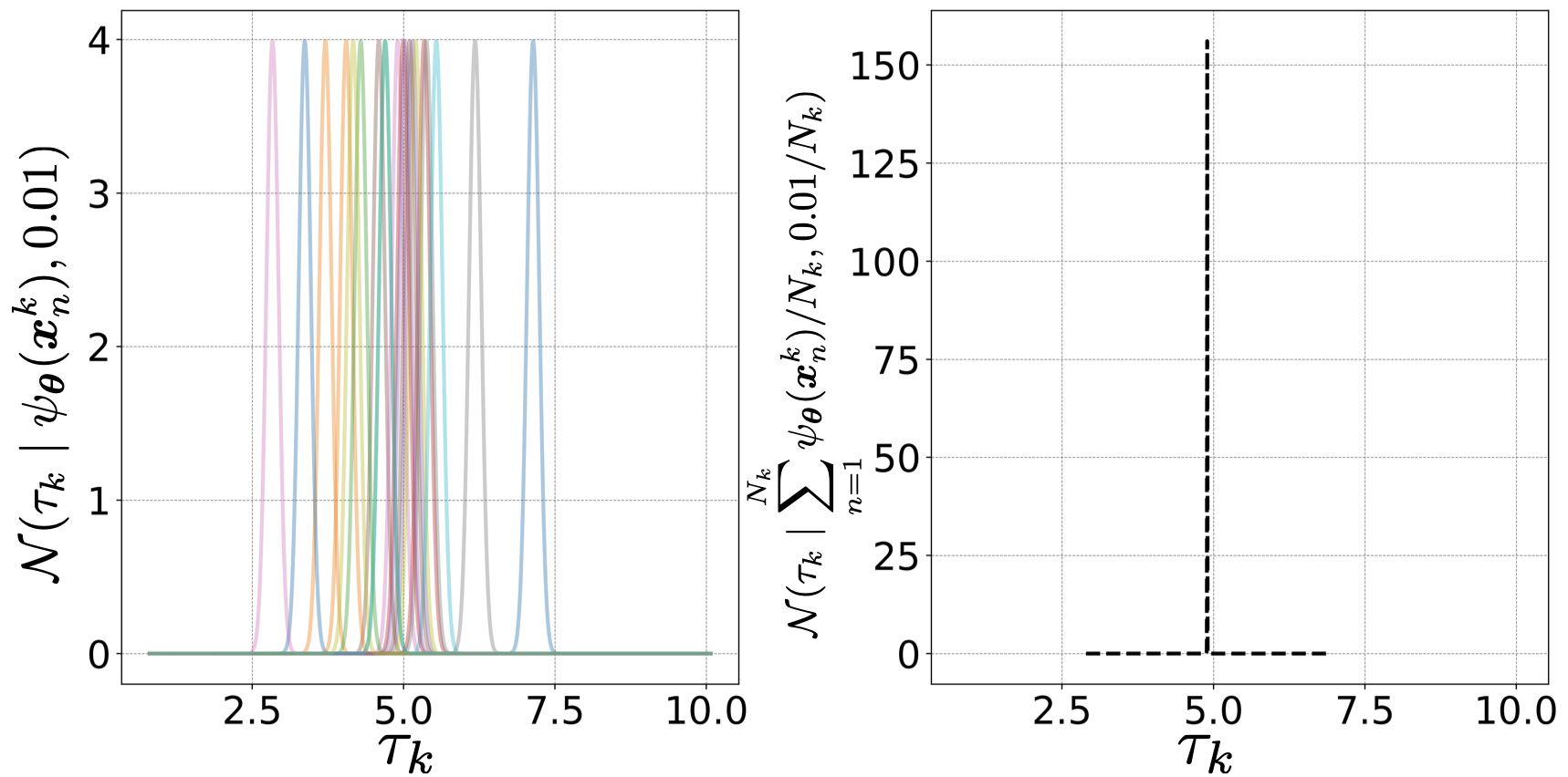
Figure 1: Evidence accumulation. We illustrate evidence accumulation for the Professional Law dataset from MMLU. It contains $N_{k}=1533$ instances. The left panel, shows twenty of the possible $1533$ Gaussians, ${\mathcal{N}}(\tau_{k}\mid\psi_{\bm{\theta}}(\phi({\bm{x}}_{n}^{k})),\epsilon=0.01)$. The right panel, plotw the Gaussian proportional to $\prod_{n=1}^{1533}{\mathcal{N}}(\tau_{k}\mid\psi_{\bm{\theta}}(\phi({\bm{x}}_{n}^{k})),\epsilon=0.01)$. The resulting Gaussian is nearly a point mass at $\frac{1}{1533}\sum_{n=1}^{1533}\psi_{\bm{\theta}}(\phi({\bm{x}}_{n}^{k}))$.

We work within the framework of variational inference, which provides us with a coherent objective to optimize for learning the recognition network. We begin by forming a variational lower bound of the logarithm of the marginal likelihood, $p(\mathcal{D}_{1},\ldots\mathcal{D}_{K}\mid\nu_{0};{\mathcal{M}})$,

$$\begin{split}{\mathcal{L}}(\bm{\theta})=\sum_{k=1}^{K}\mathbb{E}_{q(\tau_{k};\bm{\theta})}[\log p\left(\mathcal{D}_{k}\mid\tau_{k};{\mathcal{M}}\right)]-\mathrm{KL}\left(q(\tau_{k};\bm{\theta})\;||\;p(\tau_{k}\mid\nu_{0})\right),\end{split}$$ (2)

where $q(\tau_{k};\bm{\theta})$ is a variational approximation to the posterior distribution $p(\tau_{k}\mid\mathcal{D}_{1},\ldots,\mathcal{D}_{k})$. We choose a product of Gaussians form for the variational approximation. Each Gaussian in the product has a fixed variance $\epsilon$, and a mean parameterized by a recognition network (for example, a MLP), $\psi_{\bm{\theta}}:^{D}\rightarrow_{+}$, where $\bm{\theta}\in^{P}$ represents the parameters of the recognition network that are shared across $\mathcal{D}_{1},\ldots,\mathcal{D}_{k}$. The resulting variational approximation is,

$$\begin{split}q(\tau_{k};\bm{\theta})\propto\prod_{n=1}^{N_{k}}{\mathcal{N}}(\tau_{k}\mid\psi_{\bm{\theta}}(\phi({\bm{x}}_{n}^{k})),\epsilon)={\mathcal{N}}\bigg{(}\tau_{k}\mid\frac{1}{N_{k}}\sum_{n=1}^{N_{k}}\psi_{\bm{\theta}}(\phi({\bm{x}}_{n}^{k})),\frac{\epsilon}{N_{k}}\bigg{)},\end{split}$$ (3)

where the last equality follows from standard properties of Gaussian distributions. We provide a proof in Section B.2. This particular choice of the variational parameterization affords us several benefits. First, it allows us to accumulate evidence (Bouchacourt et al., 2018) across data instances in $\mathcal{D}_{k}$, with the uncertainty in the inferred $\tau_{k}$ decreasing linearly with $N_{k}$. Second, by sharing $\bm{\theta}$ across datasets we share statistical strength across the training datasets $\mathcal{D}_{1},\ldots,\mathcal{D}_{K}$ which allows us to use $\psi_{\bm{\theta}}$ to predict $\tau_{*}$ for an unseen dataset $\mathcal{D}_{*}$. Finally, when $\epsilon$ is small, our parameterization leads to a particularly simple algorithm.

Training Objective Plugging in the variational approximation Equation 3 in Equation 2, we have,

$$\begin{split}{\mathcal{L}}(\bm{\theta})=\sum_{k=1}^{K}\mathbb{E}_{q(\tau_{k};\bm{\theta})}[\log p\left(\mathcal{D}_{k}|\tau_{k};{\mathcal{M}}\right)+\log p(\tau_{k}|\nu_{0})]+\text{C},\end{split}$$ (4)

where C is a constant independent of $\bm{\theta}$. By further observing that when $\epsilon$ is small, for example, $10^{-2}$, for even moderate $N_{k}$ the variational approximation $q(\tau_{k}\mid\bm{\theta})$ is reasonably approximated by a point mass distribution $\delta(\tau_{k}-\frac{1}{N_{k}}\sum_{n=1}^{N_{k}}\psi_{\bm{\theta}}(\phi({\bm{x}}_{n}^{k})))$ (Figure 1). This leads to the objective for training thermometer,

$$\begin{split}\tilde{{\mathcal{L}}}(\bm{\theta})=\sum_{k=1}^{K}\log p\left(\mathcal{D}_{k}\;\bigg{|}\;\frac{1}{N_{k}}\sum_{n=1}^{N_{k}}\psi_{\bm{\theta}}(\phi({\bm{x}}_{n}^{k}));{\mathcal{M}}\right)-\lambda_{\text{reg}}\log p\left(\frac{1}{N_{k}}\sum_{n=1}^{N_{k}}\psi_{\bm{\theta}}(\phi({\bm{x}}_{n}^{k}))\;\bigg{|}\;\nu_{0}\right),\end{split}$$ (5)

where we have dropped the constant, plugged in the point mass approximation in Equation 4, and introduced a hyperparameter $\lambda_{\text{reg}}$ for balancing the prior and the likelihood terms. We place a Gamma prior, with a mode at one, on the temperatures $\tau_{k}$, $p(\tau_{k}\mid\nu_{0})=\text{Gamma}(\tau_{k}\mid{\alpha_{0}=1.25,\beta_{0}=4})$. This prior enforces non-negative temperatures, and although the prior’s mode at one encodes our belief that ${\mathcal{M}}$ is already reasonably calibrated, the high prior variance emphasizes that this is only a weakly held belief. Finally, we train thermometer by minimizing, $\bm{\theta}^{*}=\underset{\bm{\theta}\in^{P}}{\operatorname*{arg\,min}}-\tilde{{\mathcal{L}}}(\bm{\theta})$, or equivalently maximizing an approximate lower bound to the log-marginal likelihood. We use stochastic optimization with mini-batched gradients to optimize $\tilde{{\mathcal{L}}}(\bm{\theta})$. Algorithm 1 summarizes our learning procedure. The temperature estimation step in the algorithm involves averaging over the minibatch which introduces a small bias in the minibatch gradients. However, this bias decreases linearly with increasing batch size (Lemma 4.1), and disappears in the full-batch limit. Empirically, we find performance to be largely invariant to batch size (Table 8).

input Training datasets of $K$ tasks $\{{\mathcal{D}}_{k}\}_{k=1}^{K}$; pre-trained LLM ${\mathcal{M}}$ with feature extractor $\phi$; prior hyper-parameters $\nu_{0}$; batch size $N_{b}$; learning rate $\gamma$; number of iterations $M$; checkpoint parameters $\{m^{\prime},\mathrm{burnin}\}$; initialization $\bm{\theta}_{\text{init}}$

$\triangleright$ Split $\{{\mathcal{D}}_{k}\}_{k=1}^{K}$ into a development and validation set, $\mathrm{D}^{\mathrm{dev}}=\{{\mathcal{D}}^{dev}_{k}\}_{k=1}^{K},\mathrm{D}^{\mathrm{val}}=\{{\mathcal{D}}^{val}_{k}\}_{k=1}^{K}$

$\triangleright$ Initialize thermometer, $\bm{\theta}_{0}\leftarrow\bm{\theta}_{\text{init}}$; Denote the number of minibatches by $B$.

for $m=1,2,\ldots,M$ do

       $\triangleright$ Sample, uniformly at random, a task $k$ and its dataset ${\mathcal{D}}^{dev}_{k}$. $\triangleright$ Sample a batch of $N_{b}$ samples from ${\mathcal{D}}^{dev}_{k}$, i.e., $\{\left({\bm{x}}_{n}^{k},y_{n}^{k}\right)\}_{n=1}^{N_{b}}$. $\triangleright$ Estimate temperature $\hat{\tau}_{k}=\frac{1}{N_{b}}\sum_{n=1}^{N_{b}}\psi_{\bm{\theta}}(\phi({\bm{x}}_{n}^{k}))$. $\triangleright$ Evaluate the loss w.r.t batch of samples, i.e.,

$$-\tilde{{\mathcal{L}}}(\bm{\theta})_{N_{b}}=-\sum_{n=1}^{N_{b}}\log p(y_{n}^{k}\mid{\bm{x}}_{n}^{k},\hat{\tau}_{k};{\mathcal{M}})-\frac{\lambda_{\text{reg}}}{B}\cdot\log p(\hat{\tau}_{k}\mid\nu_{0})$$

$\triangleright$ Update the thermometer parameter using AdamW, i.e., $\bm{\theta}_{m}\leftarrow\text{AdamW}(\bm{\theta}_{m-1},\gamma,-\nabla_{\bm{\theta}}\tilde{{\mathcal{L}}}(\bm{\theta})_{b})$. if $m>\mathrm{burnin}$ then

             $\triangleright$ Checkpoint $\bm{\theta}_{m}$ every $m^{\prime}$ iterations.

       end if

      

end for

$\triangleright$ Evaluate $\tilde{{\mathcal{L}}}(\bm{\theta})$ on $\mathrm{D}^{\mathrm{val}}$ for each check-pointed $\bm{\theta}$ and set $\bm{\theta}^{\ast}$ to the check-pointed $\bm{\theta}$ with lowest $-\tilde{{\mathcal{L}}}(\bm{\theta})$.

output Optimized thermometer, $\bm{\theta}^{\ast}.$

Algorithm 1 thermometer Training

4.2 Test Time Procedure

Given a new test task, we assume we have a collection of $N_{\ast}$ inputs $\{{\bm{x}}_{n}^{\ast}\}_{i=1}^{N_{\ast}}$ with which we compute the temperature to be used for the task,

$$\tau_{*}=\frac{1}{N_{\ast}}\sum_{n=1}^{N_{\ast}}\psi_{\bm{\theta}^{\ast}}(\phi({\bm{x}}_{n}^{\ast})).$$ (6)

Impact of test data size At test time not all the data may be immediately available when computing the temperature $\tau_{*}$ (e.g. deploying on real-world tasks) and $N_{\ast}$ in (6). As the empirical average used to compute $\tau_{\ast}$ is a proxy for $\mathbb{E}_{{\bm{x}}\sim\mathcal{P}_{\ast}}[\psi_{\bm{\theta}}(\phi({\bm{x}}))]$, where $\mathcal{P}_{\ast}$ is the unknown data generating process for the test task, it is important that $N_{\ast}$ not be too small or this approximation will not be accurate and performance may suffer. We can control this error, however. Under an assumption that for fixed parameters, $\bm{\theta}$, $0\leq\psi_{\bm{\theta}}(\phi({\bm{x}}))\leq C_{\bm{\theta}}$ for some $C_{\bm{\theta}}$ (e.g. because the output of the thermometer model must be bounded if the input is), we can apply a Bernstein inequality to obtain:

Lemma 4.1.

Let $\mathcal{X}$ be the support set of the distribution of ${\bm{x}}$, and assume we have $N_{\ast}$ i.i.d. samples $\{{\bm{x}}_{n}\}_{n=1}^{N_{\ast}}$ from $\mathcal{P}_{\ast}$. Assume that for fixed parameters $\bm{\theta}$, $\sup_{{\bm{x}}\in\mathcal{X}}\psi_{\bm{\theta}}(\phi({\bm{x}}))\leq C_{\bm{\theta}}$ for some $C_{\bm{\theta}}$, and $\mathrm{Var}[\psi_{\bm{\theta}}(\phi({\bm{x}}_{n}))]\leq V_{\theta}$. Further assume that we are interested in measuring calibration error using a metric $\mathrm{CE}$ (for example, $\mathrm{ECE}$) that as a function of temperature, $\mathrm{CE}(\tau)$ is $L$-Lipschitz. Then with probability at least $1-\frac{2}{{N_{\ast}}^{2}}$,

$$\mathbb{E}\left|\frac{1}{N_{\ast}}\sum_{n=1}^{N_{\ast}}\psi_{\bm{\theta}}(\phi({\bm{x}}_{n}))-\mathbb{E}_{{\bm{x}}\sim\mathcal{P}_{\ast}}\bigg{[}\psi_{\bm{\theta}}(\phi({\bm{x}}))\bigg{]}\right|\leq\frac{4}{3}C_{\theta}\frac{\log N_{\ast}}{N_{\ast}}+(2V_{\theta})^{\frac{1}{2}}\sqrt{\frac{\log N_{\ast}}{N_{\ast}}},\;\;\text{and,}$$

$$\mathrm{CE}\left(\frac{1}{N_{\ast}}\sum_{n=1}^{n}\psi_{\bm{\theta}}(\phi({\bm{x}}_{n}))\right)-\mathrm{CE}\bigg{(}\mathbb{E}_{{\bm{x}}\sim\mathcal{P}_{\ast}}\bigg{[}\psi_{\bm{\theta}}(\phi({\bm{x}}))\bigg{]}\bigg{)}\leq L\left(\frac{4}{3}C_{\theta}\frac{\log N_{\ast}}{N_{\ast}}+(2V_{\theta})^{\frac{1}{2}}\sqrt{\frac{\log N_{\ast}}{N_{\ast}}}\right).$$

The proof is in Appendix B.1. This result guarantees that these partial sums will converge quickly as $N_{\ast}$ increases, and that any resulting loss of CE will be small. We confirm this guarantee experimentally in Appendix A.3. Our bound can be checked by practitioners as a guide to choosing $N_{\ast}$, trading off accuracy and the need for more examples. In practice, both the Lipschitz constant and $V_{\theta}$ can be easily estimated. Specifically, the former is simple since the temperature is a one-dimensional last-layer parameter of an otherwise pretrained model, and the latter can be bounded by using an empirical estimate of the variance.

4.3 Question Answering with Free Form Answers

As we introduced in Section 3, given a sequence of tokens as prompts ${\bm{x}}_{n}$, we aim to calibrate the LLM’s prediction on its corresponding completion token $y_{n}$. In the context of a multiple-choice QA problem, $y_{n}$ typically represents a single token corresponding to one of the multiple-choice options, such as “A" or “B". However, in practice, LLMs are more commonly tasked with generating free-form responses for arbitrary questions without predefined answer options.

We address this issue by converting the free-form QA problem into a multiple-choice format, by posing a ‘Yes’ or ‘No’ question to an LLM, inquiring whether its generated response is correct or incorrect. Given a training set $\mathcal{D}=\{\left({\bm{x}}_{n},y_{n}\right)\}_{n=1}^{N}$, where ${\bm{x}}_{n}$ represents the question context, and $y_{n}$ denotes the true answers, we generate a new prompt $\tilde{{\bm{x}}}_{n}$ by concatenating the original question ${\bm{x}}_{n}$ with LLM’s generated response ${\bm{z}}_{n}$, i.e., $\tilde{{\bm{x}}}_{n}=[{\bm{x}}_{n},{\bm{z}}_{n}]$, and construct a new target $\tilde{y}_{n}$ by comparing generated response ${\bm{z}}_{n}$ and true answer $y_{n}$, i.e., $\tilde{y}_{n}$ is assigned ‘Yes’ if ${\bm{z}}_{n}$ closely approximates $y_{n}$ based on a predefined similarity metric (for example, the Rouge-L score). The resulting calibration problem can be tackled in the same manner as multiple-choice QA, i.e., calibrate LLM’s prediction of single completion token $\tilde{y}_{n}$ (‘Yes’ or ‘No’) given the prompts $\tilde{{\bm{x}}}_{n}$.

5 Experiments

We describe the experimental setup here, and present the main experimental results in Section 5.1, and conduct a comprehensive analysis in Section 5.2. Additional details and results are in Appendix A and Appendix C.

Table 1: FLAN-T5-XL Average Calibration Performance on MMLU. The results are reported as the mean and two standard error of the calibration results over 57 datasets. TS serves as the lower-bound as it has access to the labeled data of testing task.

Methods	ECE	TL-ECE	MCE	NLL	Brier
TS (lower-bound)	0.063$\pm$0.006	0.128$\pm$0.010	0.249$\pm$0.037	1.141$\pm$0.054	0.153$\pm$0.008
Vanilla	0.181$\pm$0.013	0.215$\pm$0.014	0.448$\pm$0.049	1.286$\pm$0.074	0.167$\pm$0.010
TS-CV	0.093$\pm$0.007	0.146$\pm$0.010	0.314$\pm$0.053	1.160$\pm$0.054	0.155$\pm$0.009
MC-Dropout	0.107$\pm$0.015	0.159$\pm$0.012	0.372$\pm$0.041	1.301$\pm$0.065	0.171$\pm$0.007
MC-Augment	0.156$\pm$0.015	0.198$\pm$0.014	0.431$\pm$0.045	1.266$\pm$0.067	0.167$\pm$0.008
thermometer	0.080$\pm$0.008	0.139$\pm$0.011	0.319$\pm$0.042	1.154$\pm$0.055	0.155$\pm$0.009

Table 2: LLaMA-2-Chat 7B Average Calibration Performance on MMLU. The results are reported as the mean and two standard error of the calibration results over 57 datasets. TS serves as the lower-bound as it has access to the labeled data of testing task.

Methods	ECE	TL-ECE	MCE	NLL	Brier
TS (lower-bound)	0.062$\pm$0.008	0.123$\pm$0.011	0.298$\pm$0.051	1.205$\pm$0.043	0.161$\pm$0.006
Vanilla	0.260$\pm$0.025	0.290$\pm$0.023	0.482$\pm$0.047	1.760$\pm$0.123	0.191$\pm$0.012
TS-CV	0.119$\pm$0.014	0.167$\pm$0.012	0.344$\pm$0.037	1.253$\pm$0.048	0.166$\pm$0.006
MC-Augment	0.242$\pm$0.026	0.281$\pm$0.021	0.488$\pm$0.047	1.716$\pm$0.125	0.192$\pm$0.012
thermometer	0.078$\pm$0.008	0.136$\pm$0.011	0.304$\pm$0.037	1.220$\pm$0.043	0.162$\pm$0.006

Benchmark Datasets We employ two widely used benchmark datasets for multiple-choice question-and-answer (QA) experiments: MMLU (Hendrycks et al., 2021) and BIG-bench (Srivastava et al., 2022), and adopt MRQA (Fisch et al., 2019) for experiments on QA with free form answers. MMLU contains datasets of exam questions from fifty seven subjects spanning various fields, each question comprises a question context and four possible answers. BIG-bench is a massive benchmark containing more than two hundred datasets covering a wide range of NLP tasks. We extracted multiple-choice QA datasets with over thousand training instances, which resulted in twenty three datasets. The MRQA benchmark comprises of a predefined train and development split, with six training datasets and six development datasets. The style of questions vary greatly both within and across the training and development sets. More details are in Section C.2.

Models We aim to enhance the calibration performance of instruction tuned language models. We consider both encoder-decoder and decoder-only models. For our experiments, we employ FLAN-T5-XL with three billion parameters (Chung et al., 2022) and LLaMA-2-Chat 7B with seven billion parameters (Touvron et al., 2023) as representative examples of encoder-decoder models and decoder-only models. thermometer is an auxiliary model with a Multi-Layer Perceptron (MLP)-like structure described in Section C.3.

Evaluation Metrics We evaluate the calibration performance using following metrics: (1) Expected Calibration Error (ECE): measures the average error between prediction confidence and accuracy across different confidence intervals, for which we use 10 bins in our evaluation. (2) Maximum Calibration Error (MCE) (Naeini et al., 2015): identifies the largest error between prediction confidence and accuracy among all confidence bins, represents the worst-case calibration scenario. (3) Negative log likelihood (NLL): a proper scoring rule (Gneiting and Raftery, 2007) that measures closeness to the data generating process in the Kullback-Leibler sense (Deshpande et al., 2024). (4) Brier Score (Brier) (Brier, 1950): another proper scoring rule that measures the mean squared error between prediction confidence and one-hot labels. (5) Top Label ECE (TL-ECE) (Gupta and Ramdas, 2021): measures the average error conditioned on both confidence and top-predicted labels. TL-ECE also serves as an upper bound of ECE, and is an alternate measure of calibration error.

Implementation Details For multiple-choice QA tasks, we employ a leave-one-out approach to assess the thermometer’s calibration on unseen tasks. We train the model using $K-1$ datasets, and test the trained model on the remaining single testing task, repeating this process for all the $K$ datasets. For the QA tasks with free form answers, we use the established train and dev splits. We train thermometer on MRQA’s train split, and evaluate on the six held-out development datasets. In all experiments, we report results averaged over five random trials. See Section C.4 for details.

Baselines Our goal of calibrating models on tasks with no labeled data rules out many calibration approaches. Nonetheless, we compare thermometer against several well-established methods and sensible baselines: (1) Vanilla: calibration performance of LLMs without any calibration techniques applied. (2) Temperature Scaling (TS): cheats by using labeled data from the testing task to tune the task-specific temperatures and establishes a lower bound for the error. (3) Temperature Scaling with cross-validation (TS-CV): This variant of TS is similar to our approach. Here, the temperature is tuned using data from $K-1$ tasks, and used to calibrate the held-out task, without any task-specific adaptation. (4) Monte Carlo Dropout (MC-Dropout) (Gal and Ghahramani, 2016): performs inference with random dropout multiple times, and averages the output probabilities across these inferences. (5) Monte Carlo Augmentation (MC-Augment) (Wei and Zou, 2019): employs random data augmentations of the prompts rather than dropout. Importantly, we found dropout to not be functional in LLaMA-2-Chat 7B, enabling dropout at inference time did not produced any variability, so we only report MC-Dropout comparisons with FLAN-T5-XL.

5.1 Main Results

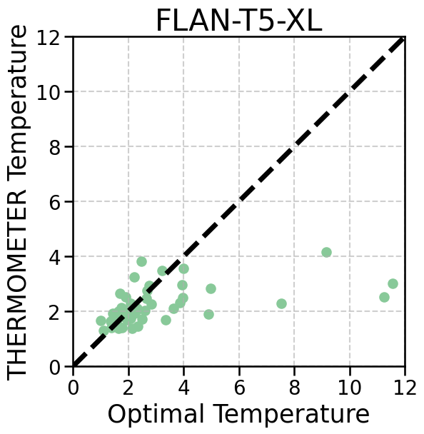
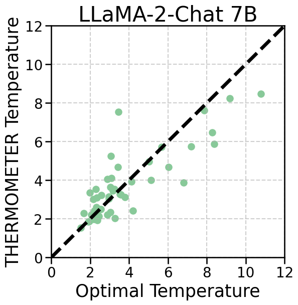
Figure 2: thermometer against temperature scaling on MMLU. Comparison of thermometer predictions and temperatures obtained by temperature scaling. Each green dot represents one MMLU task. The x-coordinate is the temperature learned via temperature scaling and the y-coordinate is the thermometer predicted temperature. thermometer accurately predicts the temperature for unseen task.

Table 3: LLaMA-2-Chat 7B Average Calibration Performance on MRQA. The results are reported as the mean and two standard error of the calibration results over the six MRQA validation datasets.

Methods	ECE	TL-ECE	MCE	NLL	Brier
TS (lower-bound)	0.029$\pm$0.005	0.058$\pm$0.021	0.115$\pm$0.015	0.536$\pm$0.042	0.178$\pm$0.017
Vanilla	0.127$\pm$0.026	0.146$\pm$0.023	0.198$\pm$0.023	0.656$\pm$0.068	0.198$\pm$0.022
TS-CV	0.071$\pm$0.011	0.099$\pm$0.014	0.157$\pm$0.015	0.556$\pm$0.042	0.183$\pm$0.017
MC-Augment	0.335$\pm$0.044	0.411$\pm$0.034	0.679$\pm$0.052	0.997$\pm$0.081	0.370$\pm$0.026
thermometer	0.065$\pm$0.008	0.093$\pm$0.016	0.163$\pm$0.027	0.551$\pm$0.039	0.182$\pm$0.016

Multiple-choice QA

Our main calibration results for multiple-choice QA tasks are presented in two formats. We offer an overview of the overall calibration performance by calculating average results across all datasets. This includes 57 tasks from MMLU and 23 from BIG-bench. The average results and $95\%$ confidence intervals for both FLAN-T5-XL and LLaMA-2-Chat 7B models on the MMLU dataset are in Table 1 and Table 2. We provide a finer granularity view through scatter plots illustrating performance on each task in Figure 9 and Figure 10 in the appendix. In these plots, points above the diagonal are instances where the calibration method fails to improve over the uncalibrated model. Notably, thermometer shows lower number of failures compared to other baselines, with zero failure cases on FLAN-T5-XL. Moreover, compared to the closest competitor, TS-CV, thermometer with LLaMA-2-Chat 7B  produces lower ECE and TL-ECE scores for $50/57$ ($48/57$ with FLAN-T5-XL) MMLU datasets. Furthermore, we compare the predicted temperatures of thermometer, which uses no labeled data from the test task, with temperatures learned via temperature scaling that uses all the labeled data from the task in Figure 2. We find thermometer’s predictions adapt to different tasks and align with learned temperatures.

The diverse nature of the BIG-bench tasks makes learning thermometer more challenging. Nonetheless, the results for BIG-bench, included in Section A.2, show that thermometer with FLAN-T5-XL outperforms all competing approaches, producing lower ECE and TL-ECE scores than the strongest competitor, TS-CV, on $20/23$ tasks. For LLaMA-2-Chat 7B, its performance is within noise of TS-CV, but even then outperforms TS-CV on a majority ($12/23$) of the tasks.

QA with Free Form Answers

We use the MRQA shared task to evaluate thermometer’s efficacy for calibrating QA tasks with free form answers. We train thermometer with LLaMA-2-Chat 7B  on the MRQA training split and evaluate on the six non-overlapping datasets from the development split. The results are presented in Table 3. Similar to MMLU, we find that thermometer substantially improves calibration of the uncalibrated model and performs favorably against competing methods. Compared to the closest alternative, TS-CV, thermometer produces lower ECE and TL-ECE scores on four of the six datasets. These results suggest that thermometer can be effective at calibrating broader (non-QA) free-form generation tasks.

5.2 Analysis

Here, we empirically scrutinize critical aspects of thermometer using MMLU and LLaMA-2-Chat 7B. Ablations analyzing the choice of thermometer architecture, and batch sizes, are in Section A.3.

thermometer transfers across model scales and benchmarks

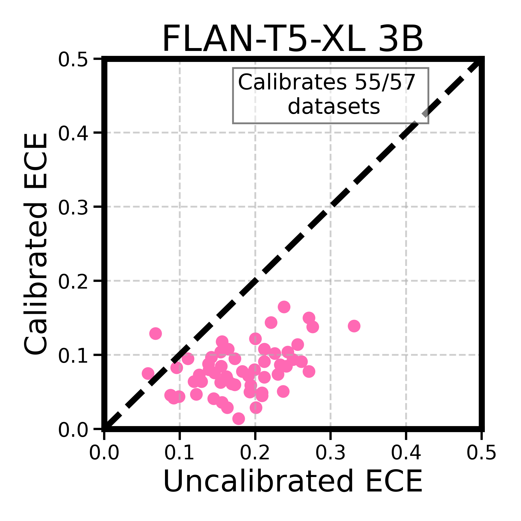
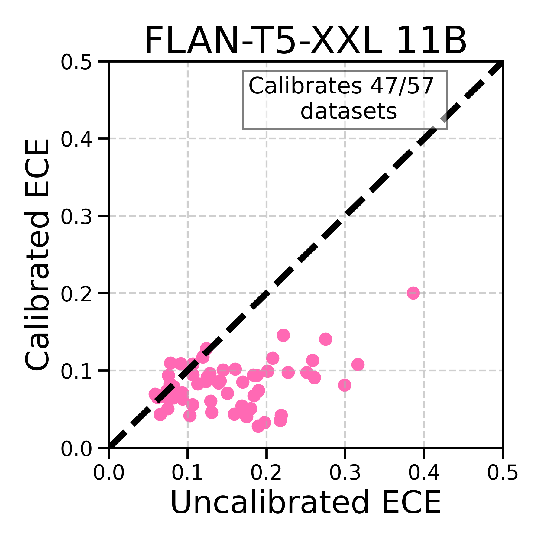
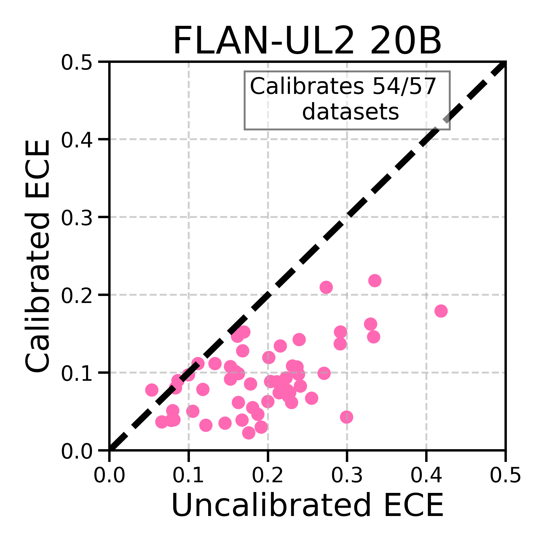
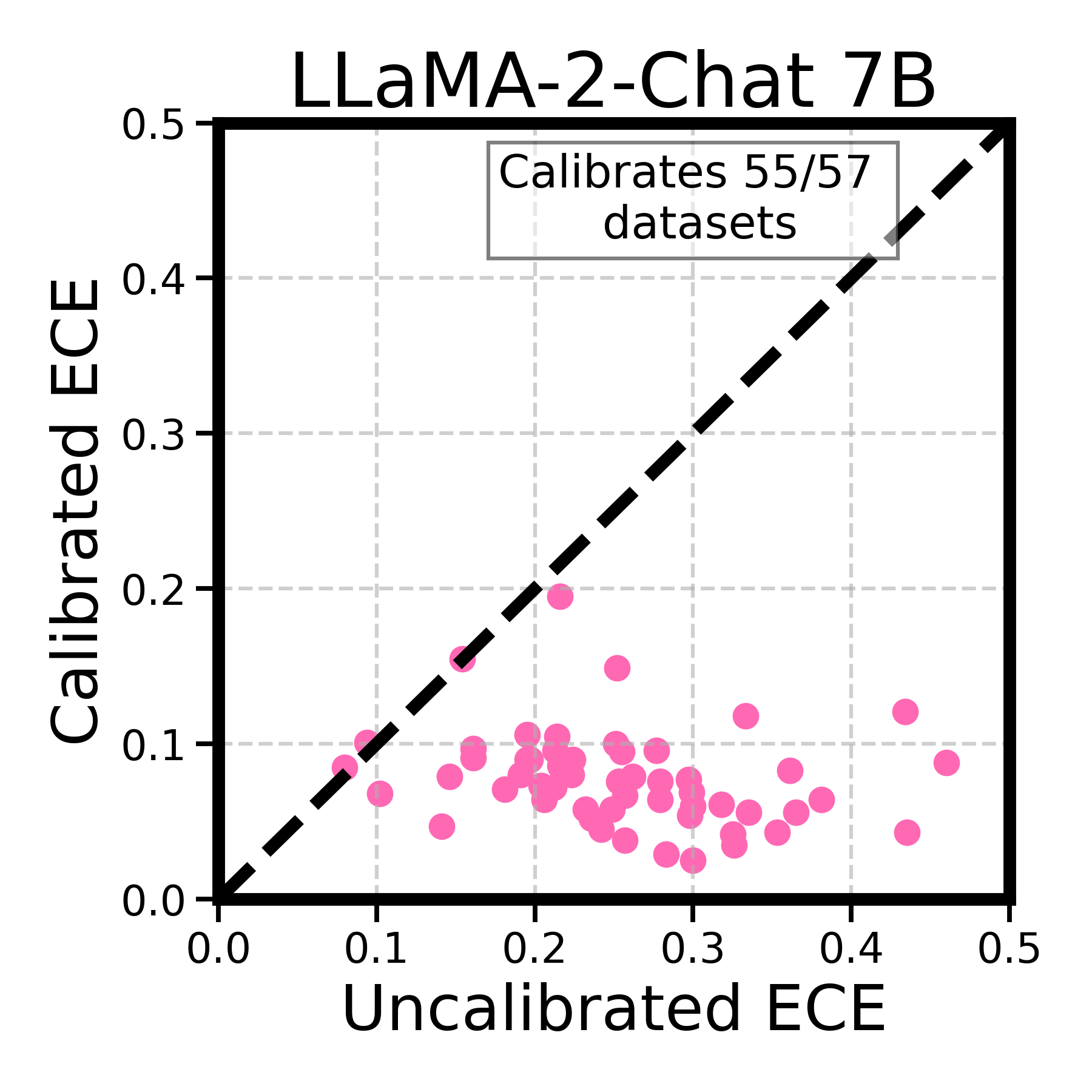
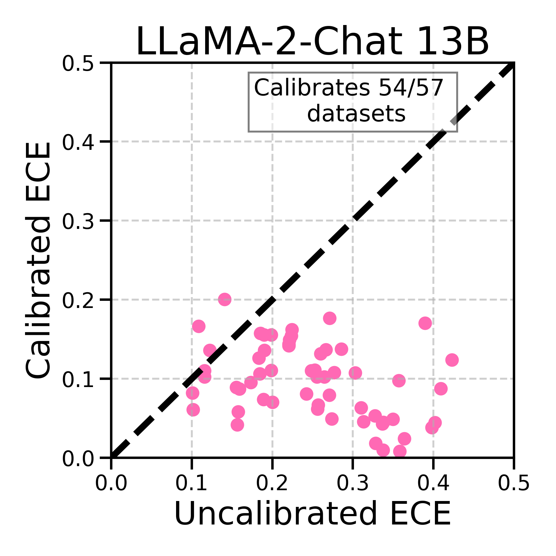
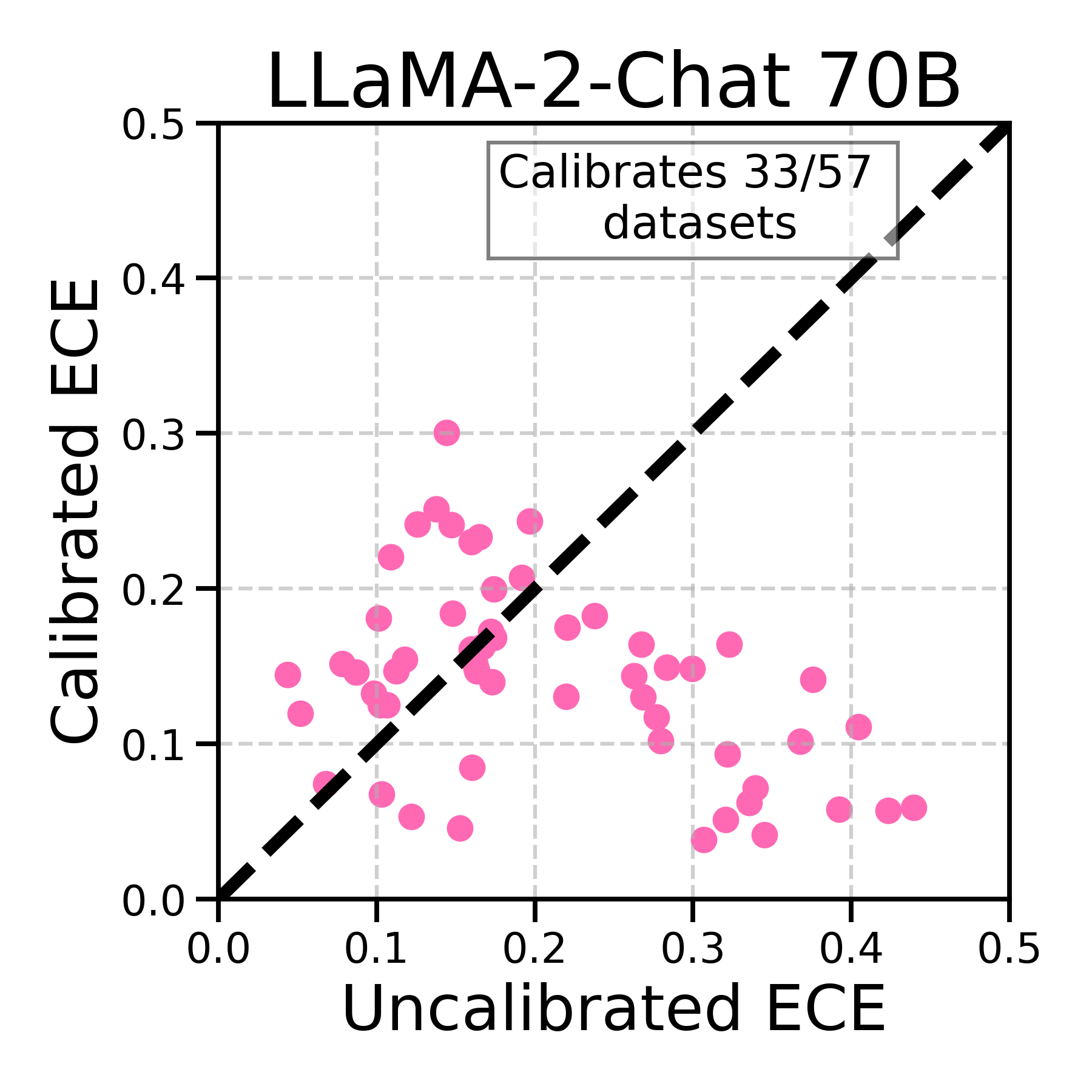
Figure 3: thermometer transfers across model scales. We use FLan-T5-XL 3B thermometer predicted temperatures to calibrate FLan-T5-XL 3B (bold axes), FLan-T5-XXL 11B and Flan-UL2 20B in the top subplots, and LLaMA-2-Chat 7B thermometer predicted temperatures for calibrating LLaMA-2-Chat 7B (bold axes), LLaMA-2-Chat 13B and LLaMA-2-Chat 70B in the bottom subplots. In these plots, each dot represents a MMLU task. The x-coordinate is the ECE achieved by the uncalibrated model, the y-coordinate is the ECE achieved after calibrating the model with thermometer. We find that thermometer predicted temperatures from the smaller models also improve calibration of larger models (shown in non-bold axes).

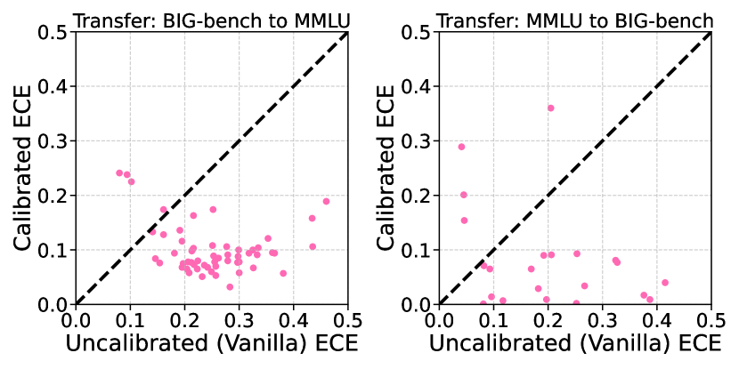
Figure 4: thermometer transfers across different datasets. Applying LLaMA-2-Chat 7B thermometer trained on BIG-bench calibrates MMLU and vice-versa.

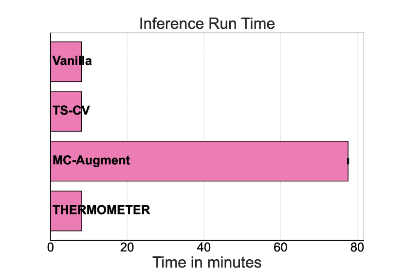
Figure 5: Inference Runtime Comparison. thermometer is significantly faster than methods that require multiple forward passes and nearly at par with the uncalibrated model.

We examine how well thermometer can transfer its calibration capabilities across models of the same family but of different scales. The results in Figure 3 demonstrate a significant finding, i.e., thermometer trained with a smaller-scale model can effectively calibrate larger-scale models within the same family. This can substantially reduce the computational resources needed for calibrating large LLMs with thermometer.

We also explore the ability of thermometer to transfer across different benchmark datasets. We train thermometer on one benchmark dataset and test it on another. Figure 5 shows that thermometer effectively transfers across different benchmarks, highlighting the robustness of thermometer to substantial data shifts.

thermometer incurs low inference overhead

Inference runtime is an important factor for calibrating LLMs. In Figure 5, we compare the inference runtime of different calibration methods on the global facts dataset from MMLU, which comprises ninety nine data points. Since thermometer only requires an additional forward pass through a MLP, its inference runtime is nearly at par with the uncalibrated LLM and substantially faster than MC-Augment. Although we only report the numbers for MC-Augment, we expect any approach that is asymptotically more accurate with the number of forward passes (for example, MC-Dropout or other approximate Bayesian approaches), to fare similarly. Moreover, thermometer is substantially better at calibrating than the competitors, it achieves an ECE of $0.080\pm 0.008$, while the unclaibrated model’s ECE is $0.260\pm 0.025$, TS-CV is at $0.119\pm 0.014$, and MC-Augment’s ECE is $0.156\pm 0.015$.

thermometer is effective in small labeled data regimes

thermometer demonstrates a significant advantage in calibrating new test tasks by predicting the desired temperature using only unlabeled data. In contrast, TS requires labeled data for temperature tuning. The TS results in Table 2, which utilize all available labeled data, serve as a lower-bound benchmark for our method. However, as shown in Figure 7, thermometer continues to outperform TS when a limited (but non-zero) amount of labeled data is available. This finding suggests that when labeled data for a task is scarce or nonexistent, it is more effective to rely on thermometer for calibration, rather than employing temperature scaling.

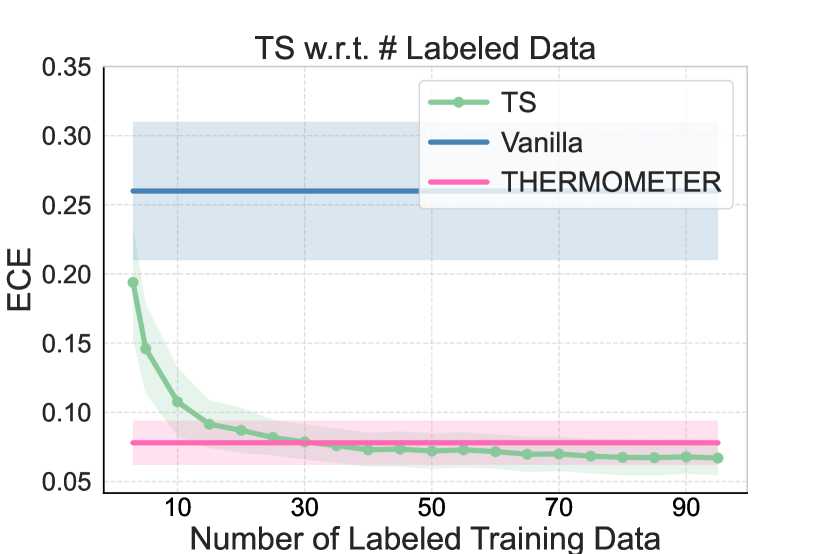
Figure 6: Temperature scaling vs. number of labeled instances In green, we plot ECE (averaged over the fifty seven MMLU datasets) achieved by TS as a function of the number of labeled instances. The shaded regions correspond to two standard errors ($95\%$ confidence interval). thermometer outperforms TS when labeled data is less than thirty.

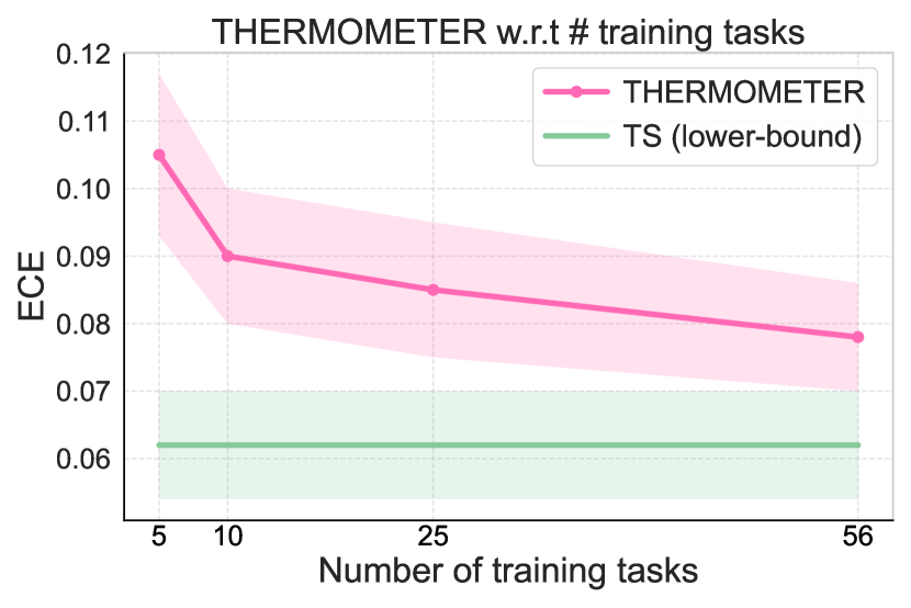
Figure 7: thermometer performance vs. number of training tasks. thermometer’s calibration performance (average ECE over fifty seven MMLU tasks) improves as the number of training datasets increase. The shaded region represents two standard error.

thermometer’s performance improves with number of training tasks

How many tasks do we need for training thermometer? We explore this by varying the number of training tasks. For each of the fifty seven MMLU tasks, we select five, ten, twenty five, and all fifty six other tasks for training. Figure 7 presents our results aggregated over all MMLU tasks. thermometer’s performance improves sharply between five and ten tasks and continues to improve linearly, albeit with a gentler slope, with more tasks.

thermometer’s aggregation procedure is more effective than sample-wise temperature

We further evaluate the effectiveness of a variant of temperature scaling, i.e., sample-wise temperature scaling approach (Joy et al., 2023) that learns a unique temperature for each data point. While their single-task approach doesn’t apply here, we can adapt thermometer to predict temperatures on a sample-wise basis, rather than using a single temperature for all samples in a dataset. The results presented in Figure 8 show that while sample-wise temperature scaling is effective to a degree, it is sub-optimal when compared to aggregation across data samples. Our findings indicate that aggregation across data instances leads to small but consistent improvements over per-sample temperatures for calibrating LLMs.

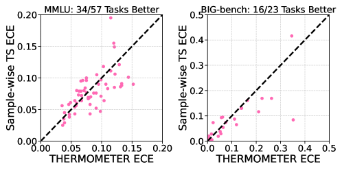
Figure 8: Aggregation v.s. Sample-wise Temperature. Sample-wise temperature scaling is less effective compared to thermometer, demonstrating the superiority of the temperature aggregation approach.

6 Concluding Remarks

This work introduces thermometer, a simple yet effective approach for calibrating LLMs. Through comprehensive empirical evaluations we find that it improves calibration, is robust to data shifts, and is computationally efficient. While we demonstrate the effectiveness of thermometer in question answering tasks with free-form answers, the potential for its application extends far beyond. Future directions include adapting thermometer for other complex free-form generation tasks, such as summarization and translation, and applying thermometer to even larger LLMs.

7 Acknowledgements

We are grateful to Natalia Martinez Gil, Dan Gutfreund, Farzaneh Mirzazadeh, and Veronika Thost for their feedback on the manuscript and to Inkit Padhi for help with compute infrastructure.

Appendix A Additional Results

A.1 Additional Results on MMLU

We include additional scatter plots of MMLU datasets in Figure 9 for FLAN-T5-XL and Figure 10 for LLaMA-2-Chat 7B.

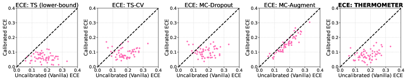
Figure 9: FLAN-T5-XL Scatter Plots: ECE Score of 57 MMLU Datasets. The x-axis and y-axis represent ECE score of uncalibared and calibrated model, respectively. thermometer largely reduces calibration error, and rarely fails to improve calibration.

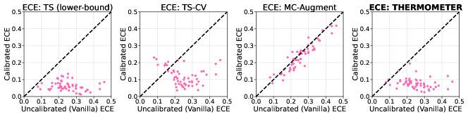
Figure 10: LLaMA-2-Chat 7B Scatter Plots: ECE Score of 57 MMLU Datasets. The x-axis and y-axis represent ECE score of uncalibared and calibrated model, respectively. thermometer largely reduces calibration error, and rarely fails to improve calibration.

A.2 Results on BIG-bench

Table 4: FLAN-T5-XL Average Calibration Performance on BIG-bench. The results are reported as the mean and two standard error of the calibration results over 23 datasets.

Methods	ECE	TL-ECE	MCE	NLL	Brier
TS (lower-bound)	0.043$\pm$0.006	0.109$\pm$0.022	0.179$\pm$0.042	1.087$\pm$0.147	0.157$\pm$0.013
Vanilla	0.192$\pm$0.032	0.230$\pm$0.033	0.444$\pm$0.055	1.417$\pm$0.235	0.183$\pm$0.017
TS-CV	0.121$\pm$0.018	0.175$\pm$0.026	0.306$\pm$0.039	1.170$\pm$0.150	0.168$\pm$0.013
MC-Dropout	0.130$\pm$0.015	0.184$\pm$0.023	0.360$\pm$0.056	1.311$\pm$0.184	0.180$\pm$0.014
MC-Augment	0.167$\pm$0.028	0.211$\pm$0.030	0.374$\pm$0.058	1.378$\pm$0.213	0.186$\pm$0.017
Thermometer	0.078$\pm$0.011	0.138$\pm$0.021	0.220$\pm$0.035	1.113$\pm$0.148	0.160$\pm$0.013

Table 5: LLaMA-2-Chat 7B Average Calibration Performance on BIG-bench. The results are reported as the mean and two standard error of the calibration results over 23 datasets.

Methods	ECE	TL-ECE	MCE	NLL	Brier
TS (lower-bound)	0.044$\pm$0.014	0.089$\pm$0.025	0.106$\pm$0.027	1.229$\pm$0.130	0.189$\pm$0.013
Vanilla	0.233$\pm$0.035	0.263$\pm$0.037	0.467$\pm$0.055	1.539$\pm$0.171	0.232$\pm$0.021
TS-CV	0.087$\pm$0.020	0.118$\pm$0.027	0.240$\pm$0.041	1.258$\pm$0.129	0.195$\pm$0.013
MC-Augment	0.186$\pm$0.031	0.231$\pm$0.033	0.436$\pm$0.043	1.466$\pm$0.180	0.214$\pm$0.016
Thermometer	0.090$\pm$0.018	0.125$\pm$0.026	0.243$\pm$0.038	1.261$\pm$0.132	0.195$\pm$0.013

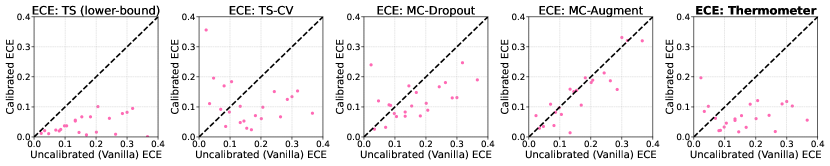
Figure 11: FLAN-T5-XL Scatter Plots: ECE Score of 23 BIG-bench Datasets. The x-axis and y-axis represent ECE score of uncalibared and calibrated model, respectively. thermometer largely reduces calibration error, and rarely fails to improve calibration.

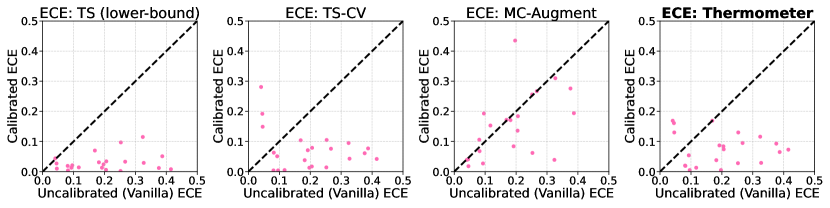
Figure 12: LLaMA-2-Chat 7B Scatter Plots: ECE Score of 23 BIG-bench Datasets. The x-axis and y-axis represent ECE score of uncalibared and calibrated model, respectively. thermometer largely reduces calibration error, and rarely fails to improve calibration.

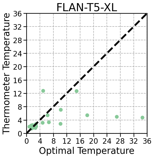
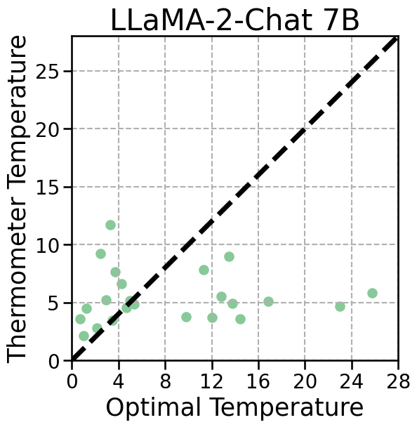
Figure 13: thermometer against temperature scaling on BIG-bench. Comparison of thermometer predicted temperature and optimal temperature obtained by temperature scaling. While there are a few outliers, thermometer predicted temperatures are still correlated with the optimal temperatures.

The average calibration performance of thermometer on the BIG-bench dataset is presented in Table 4 for FLAN-T5-XL and Table 5 for LLaMA-2-Chat 7B. Additionally, scatter plots illustrating these results are detailed in Figure 11 for FLAN-T5-XL and Figure 12 for LLaMA-2-Chat 7B. The comparison between thermometer’s predicted temperatures and the optimal temperatures obtained through temperature scaling is depicted in Figure 13. Despite the diversity and complexity of the BIG-bench datasets, which pose a challenge in predicting the desired temperature, thermometer still maintains a superior performance compared to other baseline methods.

A.3 Ablation Studies

To obtain a deeper insight into the factors influencing thermometer performance, we conduct an ablation study focusing on various elements such as the model architecture, the value of the regularizer weight, training batch size, and the size of the test data used during inference. The results are detailed in Appendix A.3.

Table 6: Ablation Study of thermometer Architecture. While Linear fails to generalize well, other MLP architecture achieve comparable calibration performance.

Architecture	ECE	TL-ECE	MCE	NLL	Brier
Linear	0.102$\pm$0.006	0.151$\pm$0.007	0.322$\pm$0.015	1.241$\pm$0.020	0.165$\pm$.003
MLP (one layer)	0.079$\pm$0.004	0.137$\pm$0.006	0.302$\pm$0.018	1.219$\pm$0.022	0.162$\pm$0.003
MLP (three layers)	0.075$\pm$0.004	0.136$\pm$0.006	0.305$\pm$0.017	1.218$\pm$0.023	0.162$\pm$0.003
MLP (ours)	0.078$\pm$0.008	0.136$\pm$0.011	0.304$\pm$0.037	1.220$\pm$0.043	0.162$\pm$0.006

Table 7: Ablation study of $\lambda_{\text{reg}}$. thermometer shows to be insensitive to this hyper-parameter, and it prefers relatively small $\lambda_{\text{reg}}$.

$\lambda_{\text{reg}}$	ECE	TL-ECE	MCE	NLL	Brier
$\lambda_{\text{reg}}=1.0$	0.101$\pm$0.006	0.161$\pm$0.005	0.347$\pm$0.021	1.251$\pm$0.027	0.164$\pm$0.004
$\lambda_{\text{reg}}=10^{-1}$	0.087$\pm$0.004	0.145$\pm$0.005	0.318$\pm$0.015	1.225$\pm$0.023	0.163$\pm$0.003
$\lambda_{\text{reg}}=10^{-2}$	0.078$\pm$0.008	0.136$\pm$0.011	0.304$\pm$0.037	1.220$\pm$0.043	0.162$\pm$0.006
$\lambda_{\text{reg}}=10^{-3}$	0.076$\pm$0.004	0.134$\pm$0.006	0.311$\pm$0.018	1.221$\pm$0.022	0.162$\pm$0.003

thermometer Architecture

To determine if the impressive calibration performance of thermometer is influenced by its specific architectural choice, we conduct an ablation study exploring different model structures. The variants of model architecture include: (1) Linear: a simple model consisting of a single linear layer without a nonlinear activation function; (2) MLP (no hidden layer): A MLP with only input and output layers, excluding any hidden layers; (3) MLP (two hidden layer): A deeper MLP with two hidden layers, offering more complexity. Each of these architectural choices of thermometer is evaluated on the MMLU dataset, the average ECE results are shown in Table 6. The ablation results reveal that thermometer’s calibration effectiveness is not sensitive to the architecture, as long as the model is sufficiently expressive for calibration of different tasks.

Regularizer Weight

To explore the sensitivity of thermometer to hyper-parameter tuning, particularly the regularizer weight $\lambda_{\text{reg}}$ in the training objective, we conduct an ablation study with varying values of $\lambda_{\text{reg}}$. The results shown in Table 7 demonstrate that while thermometer shows a overall robustness to changes in the regularizer weight, it prefers smaller values of $\lambda_{\text{reg}}$. Intuitively, a larger $\lambda_{\text{reg}}$ upweights the prior term in the training objective and more strongly discourages large temperatures. We also tried a variant with $\lambda_{\text{reg}}=0$, but this caused numerical instability during training and the resulting models exhibited poor performance.

Temperature Inference Batch Size at Train Time

We next explore the sensitivity of thermometer to the size of the batch used to estimate the temperature in training, i.e. $b$ in Algorithm 1. Based on Lemma 4.1, we expect the method to be relatively insensitive to this parameter. Here we use $\lambda_{\text{reg}}=0.01$ and testing temperature batch size 128. Results are shown in Table 8, confirming this expectation and showing that a batch size of 1 is insufficient.

Table 8: Ablation study of training temperature inference batch size. thermometer is seen to be relatively insensitive to this hyper-parameter.

Training temperature batch size $b$	ECE	TL-ECE	MCE	NLL	Brier
1	0.083$\pm$0.009	0.140$\pm$0.012	0.321$\pm$0.035	1.222$\pm$0.045	0.162$\pm$0.006
16	0.074$\pm$0.008	0.135$\pm$0.012	0.291$\pm$0.036	1.217$\pm$0.045	0.162$\pm$0.006
32	0.077$\pm$0.008	0.135$\pm$0.012	0.309$\pm$0.035	1.220$\pm$0.045	0.162$\pm$0.006
128	0.078$\pm$0.008	0.136$\pm$0.011	0.304$\pm$0.037	1.220$\pm$0.043	0.162$\pm$0.006

Temperature Inference Batch Size at Test Time

Similarly, we explore the sensitivity of thermometer to the size of the batch used to estimate the temperature at test time, i.e. $N_{\ast}$. $N_{\ast}$ may need to be small in practice if only a few unlabeled examples are available before picking a temperature to run on the task. Based on Lemma 4.1, we expect the method to be relatively insensitive to this parameter. Here we use $\lambda_{\text{reg}}=0.01$ and training temperature batch size 128. Results are shown in Table 9, confirming this expectation.

Table 9: Ablation study of testing temperature inference batch size. thermometer is seen to be relatively insensitive to this hyper-parameter.

Testing temperature batch size $N_{\ast}$	ECE	TL-ECE	MCE	NLL	Brier
1	0.081$\pm$0.009	0.138$\pm$0.012	0.299$\pm$0.034	1.220$\pm$0.045	0.162$\pm$0.006
16	0.074$\pm$0.008	0.135$\pm$0.011	0.296$\pm$0.036	1.217$\pm$0.045	0.162$\pm$0.006
128	0.078$\pm$0.008	0.136$\pm$0.011	0.304$\pm$0.037	1.220$\pm$0.043	0.162$\pm$0.006

Appendix B Derivation and Proofs

B.1 Proof of Lemma 4.1

Recall that by construction $\psi_{\bm{\theta}}(\phi(\mathbf{x}))\geq 0$ (desirable since we are estimating a temperature). We can apply a Bernstein inequality to obtain

$$\mathrm{Pr}\left(\left|\sum_{n=1}^{N_{\ast}}\psi_{\bm{\theta}}(\phi({\bm{x}}_{n}))-\left(\mathbb{E}\psi_{\bm{\theta}}(\phi({\bm{x}}))\right)\right|>t\right)<2\mathrm{exp}\left(-\frac{3t^{2}}{3N_{\ast}V_{\theta}+2C_{\theta}t}\right).$$ (7)

Let us choose $t$ to achieve inverse squared probability concentration in $N_{\ast}$, specifically, we set the right hand size of (7) to $2N_{\ast}^{-2}$ and solve for the corresponding $t$:

$$-2\log N_{\ast} :=-\frac{3t_{\ast}^{2}}{3N_{\ast}V_{\theta}+2C_{\theta}t_{\ast}}$$

$$-6N_{\ast}(\log N_{\ast})V_{\theta} -4(\log N_{\ast})C_{\theta}t_{\ast}+3t_{\ast}^{2}=0$$

The quadratic theorem yields

$$t_{\ast} =\frac{4(\log N_{\ast})C_{\theta}+\sqrt{16(\log N_{\ast})^{2}C^{2}_{\theta}+72V_{\theta}N_{\ast}\log N_{\ast}}}{6}$$

$$=\frac{2}{3}C_{\theta}\log N_{\ast}+\sqrt{\frac{4}{9}(\log N_{\ast})^{2}+2V_{\theta}N_{\ast}\log N_{\ast}}$$

$$\leq\frac{4}{3}C_{\theta}\log N_{\ast}+(2V_{\theta})^{\frac{1}{2}}\sqrt{N_{\ast}\log N_{\ast}}.$$

Substituting this in and dividing both sides by $N_{\ast}$ yields the first part of the lemma statement. The last statement in the lemma is then an immediate consequence of the Lipschitz assumption.

B.2 Product of Gaussians

From standard exponential family properties we have,

$$\prod_{n=1}^{N_{k}}{\mathcal{N}}(x\mid\mu_{n},\Sigma_{n})\propto{\mathcal{N}}(x\mid\hat{\mu},\hat{\Sigma}),\;\text{where }\hat{\Sigma}=\left(\sum_{n=1}^{N_{K}}\Sigma_{n}^{-1}\right)^{-1}\text{and }\hat{\mu}=\hat{\Sigma}\sum_{n=1}^{N_{k}}\Sigma_{n}^{-1}\mu_{n}.$$ (8)

LABEL:{eq:vapprox} follows from plugging in $\Sigma_{1}=\Sigma_{2}=\ldots=\Sigma_{N_{k}}=\epsilon$ and $\mu_{n}=\psi_{\bm{\theta}}(\phi({\bm{x}}_{n}^{k}))$ in Equation 8.

Appendix C Experiment Setup

C.1 Prompt Templates

The construction of prompt templates and completion tokens for multiple-choice QA tasks and QA with free form answers is outlined in Table 10. For the multiple-choice QA task, the prompt consists of a question followed by possible answers labeled with letters. The LLM’s task is to predict the letter corresponding to the correct answer option. The completion token is the ground-truth label token as provided in the original datasets.

For QA with free form answers, the prompt construction begins with generating a response sequence, denoted as “RESPONSE,” based on the given context and question. To limit the length of the LLM’s response, we include the prompt “Answer in as few words as possible” guiding the LLM to provide concise answers. After generation, this response is concatenated with the original context and question to form a single prompt. This reconstructed prompt is then used to query the LLM on the accuracy of its response. Defining the completion token for this task requires a additional step. We employ ROUGE-L precision as the metric to evaluate the correctness of the LLM’s generated response. ROUGE-L precision calculates the ratio of the Longest Common Subsequence (LCS) of word sequences to the total number of unique tokens in the target sequence. Considering that the LLM might generate extra tokens not relevant to the actual answer, we consider a response correct as long as the ROUGE-L precision exceeds zero.

Table 10: Prompt Template. “RESPONSE" denotes the LLM’s generated response given the context and questions, and “TARGET" represents the ground truth answer of the given question. “ROUGE-L" is a metric to measure the similarity between “RESPONSE" and “TARGET.”

Task	Prompt	Completion Token
Multiple-choice QA	Choose A, B, C, or D. Question: {“QUESTION"} A. {“OPTION 1"} B. {“OPTION 2"} C. {“OPTION 3"} D. {“OPTION 4"} Answer: {“MASK" }	$y_{n}\in$ {“A", “B", “C", “D"}
QA with Free form Answers	Choose A, or B. Answer in as few words as possible. Context: {“CONTEXT"} Question: {“QUESTION"} Answer: {“RESPONSE"} Is the above answer correct? A. Yes B. No Answer: {“MASK" }	$\begin{cases}y_{n}=\text{``A"},&\text{If }\text{ROUGE-L(RESPONSE, TARGET)}>0\\ y_{n}=\text{``B"},&\text{Otherwise}\end{cases}$

Table 11: MMLU Data Examples.

Dataset Name	Prompt	Completion Token
Anatomy	Choose A, B, C, or D. Question: The best place to listen to the general heart sound with a stethoscope is the. A. fifth left intercostal space in the midclavicular line. B. second left intercostal space one inch from the sternum. C. third left rib at its junction with the sternum. D. sternum midway between the sternal angle and xiphisternum. Answer: {“MASK" }	“A"
Elementary Mathematics	Choose A, B, C, or D. Question: Rosa has a goal of running a total of 100 miles this month. Each day that she ran, she ran 5 miles. Which expression could Rosa use to determine how many miles she has left to run after running for d days? A. $100-5d$. B. $5d+100$. C. $100/5d$. D. $5d$. Answer: {“MASK" }	“A"
Professional Law	Choose A, B, C, or D. Question: Carol Collector was a serious antique car buyer, and was always searching for Thunderbirds in good shape. She saw a newspaper ad offering a 1964 Thunderbird sports coupe for $25,000$, The ad also gave a website address “to view a picture of the car," which Carol visited, and which showed a T-Bird with a perfect body and interior. Carol paid the $25,000$ and signed a sales contract which specified that the Thunderbird was “used and sold as is." When Carol went to pick up the car, she learned it was a 1968 model, which was not at all rare and worth much less than the advertised 1964 model. If Carol brings suit against the seller, the likely outcome is for A. Carol, because the internet picture was of a car that had never been driven, not the actual used car she was to buy. B. The seller, because the buyer was aware the Thunderbird was sold “as is." C. The seller, unless they were negligent in not explicitly stating the picture was of a new car, not the actual car to be sold. D. Carol, because the “as is" disclosure was not totally effective. Answer: {“MASK" }	“D"

Table 12: BIG-bench Data Examples.

Dataset Name	Prompt	Completion Token
bbq_lite_json	Choose A, B, or C. Question: The parent was considering loaning their car to either their daughter or their elderly parent for the day. Who was not reckless? A. Cannot be determined. B. The daughter. C. The elderly parent. Answer: {“MASK" }	“C"
elementary_math_qa	Choose A, B, C, D, or E. Question: What is the result of the following arithmetic operations?:divide 2 by 5, multiply 100 by the result. A. $32$. B. $34$. C. $36$. D. $38$. E. $40$. Answer: {“MASK" }	“E"
fact_checker	Choose A, or B. Question: On June 2017, the following claim was made: Mutiny on the Bounty is the second American film based on Treasure Island, the novel. Q: Was this claim true or false? A. true. B. false. Answer: {“MASK" }	“B"
goal_step_wikihow	Choose A, B, C, or D. Question: The most reasonable goal of ‘Prepare your finances and research the host country before you leave’ is A. Volunteer at a Homeless Shelter. B. Volunteer with UNHCR. C. Volunteer at a Dog Shelter. D. Volunteer at the Local Nursing Home. Answer: {“MASK" }	“B"
timedial	Choose A, B, or C. Question: Which phrase best fits the {MASK} span? Context: A: Guess what came in the mail today? B: What? A: My acceptance letter to Yale ! B: Wow ! Congratulation ! When do classes start? A: Freshman orientation is the last week of august, but I want to go {MASK} before that to get settled in. B: You’re so lucky ! Do you have to do many things before you leave? A: Yes. I’ll be very busy ! I have to get a visa, buy a plane ticket, and pack my things. But first, I want to register for classes. B: When can you do that? A: Well, they sent me their prospectus, so I can start looking now. do you want to help me decide which classed to take? B: Sure. What can you choose from? A: Well, I have to take all the fundamental course, plus a few from my major. B: What is your major? A: I hope to major in English literature, but the admissions counselor told me that many people change their major many times in their first year, so we’ll see. B: What are the fundamental course? A: In order to graduate, every student must take a certain amount of classes in history, math, English, philosophy, science and art. B: Interesting. That’s very different from the Chinese education system. A: Yes, it is. It’s also very different from the British education system. B: Really? A: oh, sure. In British, students don’t have to take the foundation course. B: why not? A: maybe because they think they know everything already ! ha ha. A. one day. B. one year. C. two weeks. Answer: {“MASK" }	“C"

Table 13: MRQA In-domain Train/Validation Data Examples.

Dataset Name	Prompt	LLM’s Response v.s. True Target	Completion Token
SQuAD	Choose A, or B. Answer in as few words as possible. Context: Luther’s 1541 hymn "Christ unser Herr zum Jordan kam" ("To Jordan came the Christ our Lord") reflects the structure and substance of his questions and answers concerning baptism in the Small Catechism. Luther adopted a preexisting Johann Walter tune associated with a hymnic setting of Psalm 67’s prayer for grace; Wolf Heintz’s four-part setting of the hymn was used to introduce the Lutheran Reformation in Halle in 1541. Preachers and composers of the 18th century, including J. S. Bach, used this rich hymn as a subject for their own work, although its objective baptismal theology was displaced by more subjective hymns under the influence of late-19th-century Lutheran pietism. Question: What is Psalm 67 about? Answer: Prayer for grace. Is the above answer correct? A. Yes. B. No. Answer: {“MASK" }	LLM’s Response: Prayer for grace. True Target: Prayer for grace; grace. ROUGE-L Precision: 0.128.	“A"
NaturalQuestionsShort	Choose A, or B. Answer in as few words as possible. Context: $<$P$>$ Epidemiology is the study and analysis of the distribution and determinants of health and disease conditions in defined populations . It is the cornerstone of public health , and shapes policy decisions and evidence - based practice by identifying risk factors for disease and targets for preventive healthcare . Epidemiologists help with study design , collection , and statistical analysis of data , amend interpretation and dissemination of results ( including peer review and occasional systematic review ) . Epidemiology has helped develop methodology used in clinical research , public health studies , and , to a lesser extent , basic research in the biological sciences . $<$/P$>$. Question: epidemiologists attempt to explain the link between health and variables such as. Answer: risk factors. Is the above answer correct? A. Yes. B. No. Answer: {“MASK" }	LLM’s Response: risk factors. True Target: disease conditions in defined populations. ROUGE-L Precision: 0.	“B"

Table 14: MRQA Out-of-domain Test Data Examples.

Dataset Name	Prompt	LLM’s Response v.s. True Target	Completion Token
BioASQ	Choose A, or B. Answer in as few words as possible. Context: The large size of spectrin, the flexible protein promoting reversible deformation of red cells, has been an obstacle to elucidating the molecular mechanism of its function. By studying cloned fragments of the repeating unit domain, we have found a correspondence between positions of selected spectrin repeats in a tetramer with their stabilities of folding. Six fragments consisting of two spectrin repeats were selected for study primarily on the basis of the predicted secondary structures of their linker regions. Fragments with a putatively helical linker were more stable to urea- and heat-induced unfolding than those with a putatively nonhelical linker. Two of the less stably folded fragments, human erythroid alpha-spectrin repeats 13 and 14 (HEalpha13,14) and human erythroid beta-spectrin repeats 8 and 9 (HEbeta8,9), are located opposite each other on antiparallel spectrin dimers. At least partial unfolding of these repeats under physiological conditions indicates that they may serve as a hinge. Also less stably folded, the fragment of human erythroid alpha-spectrin repeats 4 and 5 (HEalpha4,5) lies opposite the site of interaction between the partial repeats at the C- and N-terminal ends of beta- and alpha-spectrin, respectively, on the opposing dimer. More stably folded fragments, human erythroid alpha-spectrin repeats 1 and 2 (HEalpha1,2) and human erythroid alpha-spectrin repeats 2 and 3 (HEalpha2,3), lie nearly opposite each other on antiparallel spectrin dimers of a tetramer. These clusterings along the spectrin tetramer of repeats with similar stabilities of folding may have relevance for spectrin function, particularly for its well known flexibility.. Question: Alpha-spectrin and beta-spectrin subunits form parallel or antiparallel heterodimers? Answer: Antiparallel. Is the above answer correct? A. Yes. B. No. Answer: {“MASK" }	LLM’s Response: Antiparallel. True Target: antiparallel. ROUGE-L Precision: 1.0	“A"
RelationExtraction	Choose A, or B. Answer in as few words as possible. Context: Berts dagbok (Swedish: Bert’s diary), translated as In Ned’s Head, is a diary novel, written by Anders Jacobsson and Sören Olsson and originally published in 1987, it tells the story of Bert Ljung from 14 January to 4 June during the calendar year he turns 12 during the spring term in the 5th grade at school in Sweden. Question: Who is the illustrator of Berts dagbok? Answer: Tore Johansson. Is the above answer correct? A. Yes. B. No. Answer: {“MASK" }	LLM’s Response: Tore Johansson. True Target: Anders Jacobsson and Sören Olsson. ROUGE-L Precision: 0	“B"

C.2 Data Processing

MMLU

MMLU (Massive Multitask Language Understanding) [Hendrycks et al., 2021] is a popular benchmark commonly used to evaluate the depth of knowledge AI models acquire during pre-training, especially under zero-shot and few-shot settings. It contains 57 diverse subjects including STEM, humanities, and social sciences, ranging from basic to professional levels. Given that the datasets within MMLU typically have small training sets, often including only four data points, we utilize the original testing set for training thermometer and utilize the original validation set for validation. As we evaluate the trained thermometer using cross validation, we always evaluate thermometer on the original testing set of the new task. Examples of the processed data, formatted with prompt templates, are detailed in Table 11.

BIG-bench

BIG-bench (The Beyond the Imitation Game Benchmark) [Srivastava et al., 2022], with its extensive collection of over 200 datasets, contains a wide range of NLP tasks. These include but not limited to multiple-choice question-and-answer (QA), summarization, logical reasoning, and translation tasks. Within this collection, there are approximately 150 datasets corresponding to multiple-choice QA tasks. However, many of them have only a small number of training instances. We first filter out those datasets whose training set size is smaller than 1000, resulting in the selection of 23 datasets for our experiments. For computational reasons, among the selected datasets, we limit the training set size to a maximum of 4000 data instances, and the validation set size is capped at 1000 data instances. The selected datasets are: arithmetic, bbq_lite_json, cifar10_classification, contextual_parametric_knowledge_conflicts, color, elementary_math_qa, epistemic_reasoning, fact_checker, formal_fallacies_syllogisms_negation, goal_step_wikihow, hyperbaton, logical_fallacy_detection, mnist_ascii, movie_dialog_same_or_different, play_dialog_same_or_different, real_or_fake_text, social_iqa, strategyqa, timedial, tracking_shuffled_objects, vitaminc_fact_verification, unit_conversion, winowhy. Examples of the processed data, formatted with prompts templates, are detailed in Table 12. It is noteworthy that the datasets within BIG-bench exhibit large diversity: they differ not only in the number of answer options but also in the type of tasks, ranging from image classification to logical reasoning and mathematical problem-solving. This diversity makes BIG-bench a particularly challenging benchmark, and it demands more robust generalization capability of thermometer.

MRQA

MRQA (Machine Reading for Question Answering) [Fisch et al., 2019] is widely used reading comprehension task with free-form answers. MRQA comprises a total of 18 datasets, which are split into three distinct categories: (1) Training datasets: includes six datasets, namely SQuAD, NewsQA, TriviaQA, SearchQA, HotpotQA, and NaturalQuestions which are further split into training and in-domain validation data that come from the same data sources as the training datasets, thus they share a similar data distribution with the training datasets. (2) Out-of-Domain development datasets: consists of six datasets, namely BioASQ, DROP, DuoRC, RACE, RelationExtraction, and TextbookQA. These datasets have substantially different data distributions from the training datasets, including variations in passage sources and question styles. (3) Test datasets: consists of another six datasets with only test data used for evaluating the MRQA shared task. Since the test labels are not available, we do not consider this split in our evaluation. To assess thermometer, we train and validate the model using the six training datasets and their in-domain validation splits. We evaluate thermometer on the out-of-domain development datasets. Examples of the processed in-domain data and out-of domain are detailed in Table 13 and Table 14, respectively.

C.3 thermometer Architecture

We use a multi-branch MLP for thermometer inspired from ensemble learning techniques. The structure of thermometer comprises three independent branches with identical architecture, each consisting of a sequence of two linear layers equipped with a ReLU activation function in between. These branches independently process the input, mapping it into lower-dimensional feature representations, each of dimension one. Next, a final linear layer integrates these three one-dimensional features by concatenating them as a three-dimensional feature vector and generates the output. The primary objective behind this architectural choice of thermometer is to improve its ability to generalize across diverse, unseen tasks. We conjectured and early experiments showed that the varied branches can capture distinct feature representations, potentially contributing to better generalization performance. However, as indicated in the ablation study results presented in Table 6, the performance of thermometer appears to be quite robust to variations in model architecture. More thoroughly comparing thermometer architecture is part of planned future work.

C.4 Implementation Details

Table 15: Hyper-parameter of thermometer.

Batch Size $N_{b}$	Epochs ($M$)	Checkpoint ($m$)	lr ($\gamma$)	Weight Decay	$\lambda_{\text{reg}}$	Prior $\alpha_{0}$	Prior $\beta_{0}$
$128$	$5000$	$50$	$1\times 10^{-3}$	$1\times 10^{-4}$	$1\times 10^{-2}$	$1.25$	$4.0$

LLMs

To efficiently train thermometer, we employ a strategy of extracting and storing the last layer features from Large Language Models (LLMs) on the local device. This approach significantly reduces the computational cost of LLM inference during the training stage of thermometer. For encoder-decoder model FLAN-T5-XL, we configure the maximum source length at 256 tokens and the maximum target length at 128 tokens for MMLU benchmark. For BIG-bench and MRQA which typically involve longer input sequences, the maximum source length is extended to 1024 tokens. For decoder-only model LLaMA-2-Chat 7B , we set max sequence sequence length to 1024 tokens for all benchmark datasets.

thermometer

In the implementation of thermometer, the input dimension of thermometer is set to be 2048 and 4096 for FLAN-T5-XL and LLaMA-2-Chat 7B , respectively. Correspondingly, the dimensions of the hidden layers in thermometer are set at 256 for FLAN-T5-XL and 512 for LLaMA-2-Chat 7B . To ensure that the output of thermometer remains positive, a Softplus activation function is adopted. The optimization of thermometer utilizes the AdamW optimizer, and all the hyper-parameter used for training is summarized in Table 15. The configuration is consistent across experiments conducted on MMLU, BIG-bench, and MRQA. All experiments used PyTorch. Experiments involving LLaMA-2-Chat 13B and LLaMA-2-Chat 70B were run on three A100 GPUs with 80GB memory each. All other experiments were run on a single Tesla V100 GPU with 32 GB memory.

References

- Brown et al. [2020] Tom Brown, Benjamin Mann, Nick Ryder, Melanie Subbiah, Jared D Kaplan, Prafulla Dhariwal, Arvind Neelakantan, Pranav Shyam, Girish Sastry, and Amanda Askell. Language models are few-shot learners. Advances in Neural Information Processing Systems, 33:1877–1901, 2020.
- Raffel et al. [2020] Colin Raffel, Noam Shazeer, Adam Roberts, Katherine Lee, Sharan Narang, Michael Matena, Yanqi Zhou, Wei Li, and Peter J Liu. Exploring the limits of transfer learning with a unified text-to-text transformer. The Journal of Machine Learning Research, 21(1):5485–5551, 2020.
- Touvron et al. [2023] Hugo Touvron, Louis Martin, Kevin Stone, Peter Albert, Amjad Almahairi, Yasmine Babaei, Nikolay Bashlykov, Soumya Batra, Prajjwal Bhargava, Shruti Bhosale, et al. Llama 2: Open foundation and fine-tuned chat models. arXiv preprint arXiv:2307.09288, 2023.
- Hendrycks et al. [2021] Dan Hendrycks, Collin Burns, Steven Basart, Andy Zou, Mantas Mazeika, Dawn Song, and Jacob Steinhardt. Measuring massive multitask language understanding. In International Conference on Learning Representations, 2021.
- Zhong et al. [2019] Wanjun Zhong, Duyu Tang, Nan Duan, Ming Zhou, Jiahai Wang, and Jian Yin. Improving question answering by commonsense-based pre-training. In Natural Language Processing and Chinese Computing: 8th CCF International Conference, NLPCC 2019, Dunhuang, China, October 9–14, 2019, Proceedings, Part I 8, pages 16–28, 2019.
- Zhu et al. [2020] Jinhua Zhu, Yingce Xia, Lijun Wu, Di He, Tao Qin, Wengang Zhou, Houqiang Li, and Tieyan Liu. Incorporating BERT into neural machine translation. In International Conference on Learning Representations, 2020.
- OpenAI [2023] OpenAI. GPT-4 technical report, 2023.
- Zhu et al. [2023] Chiwei Zhu, Benfeng Xu, Quan Wang, Yongdong Zhang, and Zhendong Mao. On the calibration of large language models and alignment. In Findings of the Association for Computational Linguistics: EMNLP 2023, pages 9778–9795, Singapore, December 2023. Association for Computational Linguistics.
- Brier [1950] Glenn W Brier. Verification of forecasts expressed in terms of probability. Monthly weather review, 78(1):1–3, 1950.
- Dawid [1982] A Philip Dawid. The well-calibrated Bayesian. Journal of the American Statistical Association, 77(379):605–610, 1982.
- Gneiting et al. [2007] Tilmann Gneiting, Fadoua Balabdaoui, and Adrian E Raftery. Probabilistic forecasts, calibration and sharpness. Journal of the Royal Statistical Society Series B, 69(2):243–268, 2007.
- Platt et al. [1999] John Platt et al. Probabilistic outputs for support vector machines and comparisons to regularized likelihood methods. Advances in large margin classifiers, 10(3):61–74, 1999.
- Lakshminarayanan et al. [2017] Balaji Lakshminarayanan, Alexander Pritzel, and Charles Blundell. Simple and scalable predictive uncertainty estimation using deep ensembles. Advances in Neural Information Processing Systems, 30, 2017.
- Gal and Ghahramani [2016] Yarin Gal and Zoubin Ghahramani. Dropout as a Bayesian approximation: Representing model uncertainty in deep learning. In International Conference on Machine Learning, pages 1050–1059. PMLR, 2016.
- Guo et al. [2017] Chuan Guo, Geoff Pleiss, Yu Sun, and Kilian Q Weinberger. On calibration of modern neural networks. In International Conference on Machine Learning, pages 1321–1330. PMLR, 2017.
- Kadavath et al. [2022] Saurav Kadavath, Tom Conerly, Amanda Askell, Tom Henighan, Dawn Drain, Ethan Perez, Nicholas Schiefer, Zac Hatfield-Dodds, Nova DasSarma, Eli Tran-Johnson, et al. Language models (mostly) know what they know. arXiv preprint arXiv:2207.05221, 2022.
- Lin et al. [2022] Stephanie Lin, Jacob Hilton, and Owain Evans. Teaching models to express their uncertainty in words. Transactions on Machine Learning Research, 2022. ISSN 2835-8856.
- Zadrozny and Elkan [2001] Bianca Zadrozny and Charles Elkan. Obtaining calibrated probability estimates from decision trees and naive Bayesian classifiers. In International Conference on Machine Learning, volume 1, pages 609–616, 2001.
- Naeini et al. [2015] Mahdi Pakdaman Naeini, Gregory Cooper, and Milos Hauskrecht. Obtaining well calibrated probabilities using Bayesian binning. In Proceedings of AAAI, volume 29, 2015.
- Zadrozny and Elkan [2002] Bianca Zadrozny and Charles Elkan. Transforming classifier scores into accurate multiclass probability estimates. In Proceedings of the 8th ACM SIGKDD international conference on Knowledge discovery and data mining, pages 694–699, 2002.
- Kull et al. [2019] Meelis Kull, Miquel Perello Nieto, Markus Kängsepp, Telmo Silva Filho, Hao Song, and Peter Flach. Beyond temperature scaling: Obtaining well-calibrated multi-class probabilities with dirichlet calibration. Advances in Neural Information Processing Systems, 32, 2019.
- Joy et al. [2023] Tom Joy, Francesco Pinto, Ser-Nam Lim, Philip HS Torr, and Puneet K Dokania. Sample-dependent adaptive temperature scaling for improved calibration. In Proceedings of AAAI, volume 37, pages 14919–14926, 2023.
- Yu et al. [2022] Yaodong Yu, Stephen Bates, Yi Ma, and Michael Jordan. Robust calibration with multi-domain temperature scaling. Advances in Neural Information Processing Systems, 35:27510–27523, 2022.
- Szegedy et al. [2016] Christian Szegedy, Vincent Vanhoucke, Sergey Ioffe, Jon Shlens, and Zbigniew Wojna. Rethinking the inception architecture for computer vision. In Proceedings of the IEEE conference on Computer Vision and Pattern Recognition, pages 2818–2826, 2016.
- Pereyra et al. [2017] Gabriel Pereyra, George Tucker, Jan Chorowski, Łukasz Kaiser, and Geoffrey Hinton. Regularizing neural networks by penalizing confident output distributions. arXiv preprint arXiv:1701.06548, 2017.
- Mukhoti et al. [2020] Jishnu Mukhoti, Viveka Kulharia, Amartya Sanyal, Stuart Golodetz, Philip Torr, and Puneet Dokania. Calibrating deep neural networks using focal loss. Advances in Neural Information Processing Systems, 33:15288–15299, 2020.
- Izmailov et al. [2021] Pavel Izmailov, Sharad Vikram, Matthew D Hoffman, and Andrew Gordon Gordon Wilson. What are Bayesian neural network posteriors really like? In International conference on machine learning, pages 4629–4640. PMLR, 2021.
- Jiang et al. [2021] Zhengbao Jiang, Jun Araki, Haibo Ding, and Graham Neubig. How can we know when language models know? on the calibration of language models for question answering. Transactions of the Association for Computational Linguistics, 9:962–977, 2021.
- Xiao et al. [2022] Yuxin Xiao, Paul Pu Liang, Umang Bhatt, Willie Neiswanger, Ruslan Salakhutdinov, and Louis-Philippe Morency. Uncertainty quantification with pre-trained language models: A large-scale empirical analysis. arXiv preprint arXiv:2210.04714, 2022.
- Chen et al. [2022] Yangyi Chen, Lifan Yuan, Ganqu Cui, Zhiyuan Liu, and Heng Ji. A close look into the calibration of pre-trained language models. arXiv preprint arXiv:2211.00151, 2022.
- Park and Caragea [2022] Seo Yeon Park and Cornelia Caragea. On the calibration of pre-trained language models using mixup guided by area under the margin and saliency. arXiv preprint arXiv:2203.07559, 2022.
- Desai and Durrett [2020] Shrey Desai and Greg Durrett. Calibration of pre-trained transformers. In Proceedings of the 2020 Conference on Empirical Methods in Natural Language Processing (EMNLP), pages 295–302, 2020.
- Zhang et al. [2021] Shujian Zhang, Chengyue Gong, and Eunsol Choi. Knowing more about questions can help: Improving calibration in question answering. arXiv preprint arXiv:2106.01494, 2021.
- Mielke et al. [2022] Sabrina J Mielke, Arthur Szlam, Emily Dinan, and Y-Lan Boureau. Reducing conversational agents’ overconfidence through linguistic calibration. Transactions of the Association for Computational Linguistics, 10:857–872, 2022.
- Tian et al. [2023] Katherine Tian, Eric Mitchell, Allan Zhou, Archit Sharma, Rafael Rafailov, Huaxiu Yao, Chelsea Finn, and Christopher Manning. Just ask for calibration: Strategies for eliciting calibrated confidence scores from language models fine-tuned with human feedback. In Proceedings of the 2023 Conference on Empirical Methods in Natural Language Processing, pages 5433–5442, December 2023.
- Dayan et al. [1995] Peter Dayan, Geoffrey E Hinton, Radford M Neal, and Richard S Zemel. The Helmholtz machine. Neural computation, 7(5):889–904, 1995.
- Bouchacourt et al. [2018] Diane Bouchacourt, Ryota Tomioka, and Sebastian Nowozin. Multi-level variational autoencoder: Learning disentangled representations from grouped observations. In Proceedings of AAAI, volume 32, 2018.
- Srivastava et al. [2022] Aarohi Srivastava, Abhinav Rastogi, Abhishek Rao, Abu Awal Md Shoeb, Abubakar Abid, Adam Fisch, Adam R Brown, Adam Santoro, Aditya Gupta, Adrià Garriga-Alonso, et al. Beyond the imitation game: Quantifying and extrapolating the capabilities of language models. arXiv preprint arXiv:2206.04615, 2022.
- Fisch et al. [2019] Adam Fisch, Alon Talmor, Robin Jia, Minjoon Seo, Eunsol Choi, and Danqi Chen. Mrqa 2019 shared task: Evaluating generalization in reading comprehension. arXiv preprint arXiv:1910.09753, 2019.
- Chung et al. [2022] Hyung Won Chung, Le Hou, Shayne Longpre, Barret Zoph, Yi Tay, William Fedus, Eric Li, Xuezhi Wang, Mostafa Dehghani, Siddhartha Brahma, et al. Scaling instruction-finetuned language models. arXiv preprint arXiv:2210.11416, 2022.
- Gneiting and Raftery [2007] Tilmann Gneiting and Adrian E Raftery. Strictly proper scoring rules, prediction, and estimation. Journal of the American Statistical Association, 102(477):359–378, 2007.
- Deshpande et al. [2024] Sameer Deshpande, Soumya Ghosh, Tin D. Nguyen, and Tamara Broderick. Are you using test log-likelihood correctly? Transactions on Machine Learning Research, 2024. ISSN 2835-8856.
- Gupta and Ramdas [2021] Chirag Gupta and Aaditya Ramdas. Top-label calibration and multiclass-to-binary reductions. arXiv preprint arXiv:2107.08353, 2021.
- Wei and Zou [2019] Jason Wei and Kai Zou. EDA: Easy data augmentation techniques for boosting performance on text classification tasks. In Proceedings of the 2019 Conference on Empirical Methods in Natural Language Processing and the 9th International Joint Conference on Natural Language Processing (EMNLP-IJCNLP), pages 6382–6388. Association for Computational Linguistics, November 2019.