Solutions of tetrahedron equation from quantum cluster algebra associated with symmetric butterfly quiver

Abstract.

We construct a new solution to the tetrahedron equation by further pursuing the quantum cluster algebra approach in our previous works. The key ingredients include a symmetric butterfly quiver attached to the wiring diagrams for the longest element of type $A$ Weyl groups and the implementation of quantum $Y$-variables through the $q$-Weyl algebra. The solution consists of four products of quantum dilogarithms, incorporating a total of seven parameters. By exploring both the coordinate and momentum representations, along with their modular double counterparts, our solution encompasses various known three-dimensional (3D) $R$-matrices. These include those obtained by Kapranov-Voevodsky (’94) utilizing the quantized coordinate ring, Bazhanov-Mangazeev-Sergeev (’10) from a quantum geometry perspective, Kuniba-Matsuike-Yoneyama (’23) linked with the quantized six-vertex model, and Inoue-Kuniba-Terashima (’23) associated with the Fock-Goncharov quiver. The 3D $R$-matrix presented in this paper offers a unified perspective on these existing solutions, coalescing them within the framework of quantum cluster algebra.

1. Introduction

The tetrahedron equation [21] is a generalization of the Yang-Baxter equation [1] to three-dimensional systems. A fundamental form of the equation in the so-called vertex formulation reads

$$R_{124}R_{135}R_{236}R_{456}=R_{456}R_{236}R_{135}R_{124},$$

where $R$ is a linear operator on $V^{\otimes 3}$ for some vector space $V$, and the indices specify the tensor components in $V^{\otimes 6}$ on which it acts non-trivially.

In this paper we construct a new solution to the tetrahedron equation by an approach based on quantum cluster algebras [5, 6]. This method, initiated in [20] and further developed in [10, 11], commences with the Weyl group of type $A$ and employing wiring diagrams to represent reduced expressions of the longest element in a standard format. One introduces a specific quiver and the corresponding quantum cluster algebra linked to these wiring diagrams. The pivotal element of the approach is the cluster transformation $\hat{R}$ serving as a counterpart of the cubic Coxeter relation. It acts on quantum $Y$-variables through a sequence of mutations and permutations. From the consideration about the embedding $A_{2}\hookrightarrow A_{3}$, $\hat{R}$ is shown to satisfy the tetrahedron equation. Apart from the monomial part, $\hat{R}$ is described as an adjoint action of quantum dilogarithms. The next key step is to devise a realization of the quantum $Y$-variables in terms of a direct product of $q$-Weyl algebras which is an exponential version of the algebra of canonical coordinates $u_{i}$ and momenta $w_{i}$ with relations ${\mathrm{e}}^{u_{i}}{\mathrm{e}}^{w_{j}}=q^{\delta_{ij}}{\mathrm{e}}^{w_{j}}{\mathrm{e}}^{u_{i}}$, ${\mathrm{e}}^{u_{i}}{\mathrm{e}}^{u_{j}}={\mathrm{e}}^{u_{j}}{\mathrm{e}}^{u_{i}}$ and ${\mathrm{e}}^{w_{i}}{\mathrm{e}}^{w_{j}}={\mathrm{e}}^{w_{j}}{\mathrm{e}}^{w_{i}}$. It allows for the cluster transformation, including its monomial part, to be fully expressed in the adjoint form $\hat{R}=\mathrm{Ad}(R)$. It is this $R$ which has many interesting features connected to existing solutions. The operator $R$ can be endowed with several “spectral parameters” and satisfies the tetrahedron equation on its own including these parameters.

We execute the above program for the symmetric butterfly (SB) quiver, which is a symmetrized version of the butterfly quiver introduced in [20]. The vertices of an SB quiver are placed both on the vertices of the wiring diagram and within its domains. This contrasts with the Fock-Goncharov (FG) and the square quivers studied in [10] and [20, 11], respectively. In the former, vertices are assigned to the domains of the wiring diagrams, while in the latter, they are assigned to the edges.

Apart from $q={\mathrm{e}}^{\hbar}$, our $R$-matrix $R=R_{123}$ involves parameters $C_{1}$, …, $C_{8}$ subject to $C_{5}+C_{6}=C_{7}+C_{8}$. Up to normalization, it is given by

$$\begin{split}R&=\Psi_{q}({\mathrm{e}}^{2C_{7}+u_{1}+u_{3}+w_{1}-w_{2}+w_{3}})^{-1}\Psi_{q}({\mathrm{e}}^{2C_{5}+u_{1}-u_{3}+w_{1}-w_{2}+w_{3}})^{-1}\\ &\quad\times P\Psi_{q}({\mathrm{e}}^{2C_{2}+2C_{3}-2C_{6}+2C_{8}+u_{1}-u_{3}+w_{1}-w_{2}+w_{3}})\Psi_{q}({\mathrm{e}}^{2C_{2}+2C_{3}+u_{1}+u_{3}+w_{1}-w_{2}+w_{3}}),\\ P&={\mathrm{e}}^{\tfrac{1}{\hbar}(u_{3}-u_{2})w_{1}}{\mathrm{e}}^{\tfrac{1}{\hbar}\lambda_{0}(-w_{1}-w_{2}+w_{3})}{\mathrm{e}}^{\tfrac{1}{\hbar}(\lambda_{1}u_{1}+\lambda_{2}u_{2}+\lambda_{3}u_{3})}\rho_{23},\end{split}$$ (1.1)

where $\Psi_{q}$ is the quantum dilogarithm (2.6), $\lambda_{i}$’s are linear combinations of $C_{1}$, …, $C_{8}$ in (5.3), and $\rho_{23}$ is the permutation $(u_{2},w_{2})\leftrightarrow(u_{3},w_{3})$.

The result (1.1) is universal within the current approach based on the SB quiver. In fact, one can project it onto various representations of the canonical variables. Our final result for the matrix elements $\langle\mathbf{n}|R|\mathbf{n}^{\prime}\rangle$ (up to normalization) with bases labeled by $\mathbf{n}=(n_{1},n_{2},n_{3})$ and $\mathbf{n}^{\prime}=(n^{\prime}_{1},n^{\prime}_{2},n^{\prime}_{3})\in{\mathbb{Z}}^{3}$ reads

$$\begin{split}\langle\mathbf{n}|R|\mathbf{n}^{\prime}\rangle&=\delta^{n_{1}+n_{2}}_{n^{\prime}_{1}+n^{\prime}_{2}}\delta^{n_{2}+n_{3}}_{n^{\prime}_{2}+n^{\prime}_{3}}{\mathrm{e}}^{\lambda_{1}n^{\prime}_{1}+\lambda_{2}n^{\prime}_{3}+\lambda_{3}n^{\prime}_{2}}({\mathrm{e}}^{2C_{5}}q^{n_{1}+g_{3}})^{n_{3}+g_{3}}q^{n^{\prime}_{2}+g_{2}}\\ &\quad\times\oint\frac{dz}{2\pi iz^{n^{\prime}_{2}+g_{2}+1}}\frac{(-z{\mathrm{e}}^{-2C_{8}}q^{2+n^{\prime}_{1}+n^{\prime}_{3}};q^{2})_{\infty}(-z{\mathrm{e}}^{-2C_{7}}q^{-n_{1}-n_{3}};q^{2})_{\infty}}{(-z{\mathrm{e}}^{-2C_{6}}q^{n^{\prime}_{1}-n^{\prime}_{3}};q^{2})_{\infty}(-z{\mathrm{e}}^{-2C_{5}}q^{n^{\prime}_{3}-n^{\prime}_{1}};q^{2})_{\infty}}\end{split}$$ (1.2)

in the coordinate representation of the $q$-Weyl algebras where $u_{i}$ is diagonal (Theorem 5.1), and

$$\begin{split}\langle\mathbf{n}|R|\mathbf{n}^{\prime}\rangle&=q^{\psi_{0}}(-{\mathrm{e}}^{-2C_{7}})^{\frac{m_{1}}{2}}({\mathrm{e}}^{2C_{8}-2C_{3}})^{\frac{m_{2}}{2}}({\mathrm{e}}^{-C_{1}-C_{2}-2C_{3}-C_{4}})^{\frac{m_{3}}{2}}({\mathrm{e}}^{C_{1}-C_{2}-2C_{3}-C_{4}})^{\frac{m_{4}}{2}}\\ &\quad\times\frac{({\mathrm{e}}^{2C_{3}};q^{2})_{\frac{m_{1}}{2}}({\mathrm{e}}^{-2C_{2}-2C_{8}};q^{2})_{\frac{m_{2}}{2}}({\mathrm{e}}^{2C_{1}-2C_{3}+2C_{5}};q^{2})_{\frac{m_{3}}{2}}({\mathrm{e}}^{-2C_{1}-2C_{3}+2C_{6}};q^{2})_{\frac{m_{4}}{2}}}{({\mathrm{e}}^{-4C_{3}+2C_{5}+2C_{6}};q^{2})_{\frac{m_{3}+m_{4}}{2}}}\end{split}$$ (1.3)

in the momentum representation where $w_{i}$ is diagonal (Theorem 5.4). Here $(g_{1},g_{2},g_{3})=\tfrac{1}{\hbar}(C_{7}-C_{6},-C_{4},C_{7}-C_{5})$, $m_{i}$ and $\psi_{0}$ are linear and quadratic forms of $\mathbf{n}$ and $\mathbf{n}^{\prime}$ as given in (5.39) and (5.40).

Let us write (1.2) and (1.3) as $R^{n_{1},n_{2},n_{3}}_{n^{\prime}_{1},n^{\prime}_{2},n^{\prime}_{3}}$ and $S^{n_{1},n_{2},n_{3}}_{n^{\prime}_{1},n^{\prime}_{2},n^{\prime}_{3}}$, respectively. We have also evaluated the matrix elements in the modular double setting with the corresponding results $\mathcal{R}^{n_{1},n_{2},n_{3}}_{n^{\prime}_{1},n^{\prime}_{2},n^{\prime}_{3}}$ (Theorem 6.1) and $\mathcal{S}^{n_{1},n_{2},n_{3}}_{n^{\prime}_{1},n^{\prime}_{2},n^{\prime}_{3}}$ (Theorem 6.3). They are expressed in terms of the non-compact quantum dilogarithm (6.2). When the parameters are specialized appropriately, our $R$-matrices yield those obtained in [12] as the intertwiner of the quantized coordinate ring of $SL_{3}$ (see also [3, 15]), in [2] from a quantum geometry consideration, in [16] from a quantized six-vertex model, and in [10] from the quantum cluster algebra associated with the FG quiver. These results are summarized in Table 1.1.

	$\begin{matrix}\text{relevant quantum}\\ \text{dilogarithm}\end{matrix}$	coordinate rep.	momentum rep.	$\begin{matrix}\text{specialization adapted}\\ \text{to the FG quiver}\end{matrix}$
$q$-dilog $R$	$\Psi_{q}$	$R^{n_{1},n_{2},n_{3}}_{n^{\prime}_{1},n^{\prime}_{2},n^{\prime}_{3}}$, Th. 5.1	$S^{n_{1},n_{2},n_{3}}_{n^{\prime}_{1},n^{\prime}_{2},n^{\prime}_{3}}$, Th. 5.4
(5.4)	(2.6)	[12, 3], Rem. 5.3	[16], Rem. 5.5	[10], Th. 8.2
modular $\mathcal{R}$	$\Phi_{\mathfrak{b}}$	$\mathcal{R}^{n_{1},n_{2},n_{3}}_{n^{\prime}_{1},n^{\prime}_{2},n^{\prime}_{3}}$, Th. 6.1	$\mathcal{S}^{n_{1},n_{2},n_{3}}_{n^{\prime}_{1},n^{\prime}_{2},n^{\prime}_{3}}$, Th. 6.3
(6.9)	(6.2)	[2], Rem. 7.3	[16], Rem. 6.4	[10], Prop. 8.4

Table 1.1. $R$-matrices in this paper. Relations to those in the literature and the relevant remarks or statements are given in the second line within each box.

In [11], the $R$-matrix in [18] was reproduced in a parallel story based on the square quiver. Along with the current results obtained from the SB quiver, the quantum cluster algebra approach has successfully captured most of the significant solutions of the tetrahedron equation known to date for a generic $q$. Additionally, this approach has been extended to the 3D reflection equations [9, 15], as previously demonstrated with the FG quiver in [10]. In this paper we assume that $q$ is generic throughout. We hope to explore the $q$ root-of-unity case elsewhere.

The layout of the paper is as follows. In Section 2 we recall basic facts about quantum cluster algebras necessary in this paper. In Section 3 we introduce the SB quiver and study the cluster transformation $\hat{R}$. In Section 4 we realize the quantum $Y$-variables by $q$-Weyl algebras and extract $R$ such that $\hat{R}=\mathrm{Ad}(R)$. The contents of Sections 3 and 4 are parallel with [11]. The matrix elements of $R$ are calculated in Sections 5 and 6. In Section 7 we explain that the $R$-matrix in this paper satisfies the so-called $RLLL=LLLR$ relation for the $L$-operator which can be regarded as a quantized six-vertex model [16, 2]. It implies that the matrix elements obey linear recursion relations. In Section 8 we explain that the $R$-matrix for the FG quiver previously obtained in [10] arises as a special limit of the $R$-matrix in this paper. Appendix A is a supplement to Section 3.4. Appendix B provides another formula for $R$ corresponding to a different choice of signs labeling the decomposition of mutations into monomial and automorphism parts. Appendix C contains integral formulas for non-compact quantum dilogarithm. Appendix D is a list of explicit forms of the $RLLL=LLLR$ relations.

2. Quantum cluster algebra

2.1. Mutation

Let us recall the definition of quantum cluster mutation following [4]. For a finite set $I$, set $B=(b_{ij})_{i,j\in I}$ with $b_{ij}=-b_{ji}\in{\mathbb{Z}}/2$. We call $B$ the exchange matrix. In this article we will only encounter skew-symmetric exchange matrices with $b_{ij}\in\{\pm 1,\pm\frac{1}{2},0\}$. An exchange matrix will be depicted as a quiver. It is an oriented graph with vertices labeled with the elements of $I$ and a solid arrow (resp. dotted arrow) from $i$ to $j$ when $b_{ij}=1$ (resp. $b_{ij}=\frac{1}{2}$).

Let $\mathcal{Y}(B)$ be a skew field generated by $q$-commuting variables $Y=(Y_{i})_{i\in I}$ under the relations

$$Y_{i}Y_{j}=q^{2b_{ij}}Y_{j}Y_{i}.$$ (2.1)

The data $(B,Y)$ will be called a quantum $y$-seed and $Y_{i}$ a (quantum) $Y$-variable. We assume that the parameter $q$ is generic throughout. For $(B,Y)$ and $k\in I$, the mutation $\mu_{k}$ transforms $(B,Y)$ to $(B^{\prime},Y^{\prime}):=\mu_{k}(B,Y)$ where

$$b_{ij}^{\prime}=\begin{cases}-b_{ij}&i=k\text{ or }j=k,\\ \displaystyle{b_{ij}+\frac{|b_{ik}|b_{kj}+b_{ik}|b_{kj}|}{2}}&\text{otherwise},\end{cases}$$ (2.2)

$$Y_{i}^{\prime}=\begin{cases}Y_{k}^{-1}&i=k,\\ \displaystyle{Y_{i}\prod_{j=1}^{|b_{ik}|}(1+q^{2j-1}Y_{k}^{-\mathrm{sgn}(b_{ik})})^{-\mathrm{sgn}(b_{ik})}}&i\neq k.\end{cases}$$ (2.3)

The mutations are involutive, $\mu_{k}\mu_{k}=\mathrm{id.}$, and commutative, $\mu_{k}\mu_{j}=\mu_{j}\mu_{k}$ if $b_{jk}=b_{kj}=0$. The mutation $\mu_{k}$ induces an isomorphism of skew fields $\mu_{k}^{\ast}\colon\mathcal{Y}(B^{\prime})\to\mathcal{Y}(B)$, where $\mathcal{Y}(B^{\prime})$ is a skew field generated by the variables $Y^{\prime}=(Y^{\prime}_{i})_{i\in I}$ under the relations $Y^{\prime}_{i}Y^{\prime}_{j}=q^{2b^{\prime}_{ij}}Y^{\prime}_{j}Y^{\prime}_{i}$.

The map $\mu_{k}^{\ast}$ is decomposed into two parts, a monomial part and an automorphism part [5], in two ways [14]. To explain it, let us introduce an isomorphism $\tau_{k,\varepsilon}$ of the skew fields for $\varepsilon\in\{+,-\}$ by

$$\tau_{k,{\varepsilon}}:~{}\mathcal{Y}(B^{\prime})\to\mathcal{Y}(B);\quad Y^{\prime}_{i}\mapsto\begin{cases}Y_{k}^{-1}&i=k,\\ q^{-b_{ik}[{\varepsilon}b_{ik}]_{+}}Y_{i}Y_{k}^{[{\varepsilon}b_{ik}]_{+}}&i\neq k,\end{cases}$$ (2.4)

where $[a]_{+}:=\max[0,a]$. The adjoint action $\mathrm{Ad}_{k,{\varepsilon}}$ on $\mathcal{Y}(B)$ is defined by

$$\mathrm{Ad}_{k,+}:=\mathrm{Ad}(\Psi_{q}(Y_{k})),\quad\mathrm{Ad}_{k,-}:=\mathrm{Ad}(\Psi_{q}(Y_{k}^{-1})^{-1}),$$ (2.5)

where $\mathrm{Ad}(Y)(X)=YXY^{-1}$. The symbol $\Psi_{q}(Y)$ appearing here denotes the quantum dilogarithm

$$\Psi_{q}(Y)=\frac{1}{(-qY;q^{2})_{\infty}},\quad(z;q)_{\infty}=\prod_{n=0}^{\infty}(1-zq^{n}).$$ (2.6)

One has the expansions

$$\Psi_{q}(Y)=\sum_{n=0}^{\infty}\frac{(-qY)^{n}}{(q^{2};q^{2})_{n}},\qquad\Psi_{q}(Y)^{-1}=\sum_{n=0}^{\infty}\frac{q^{n^{2}}Y^{n}}{(q^{2};q^{2})_{n}},$$ (2.7)

where $(z;q^{2})_{n}=(z;q^{2})_{\infty}/(zq^{2n};q^{2})_{\infty}$ for any $n$. Basic properties of the quantum dilogarithm are

$$\Psi_{q}(q^{2}U)\Psi_{q}(U)^{-1}=1+qU,$$ (2.8)

$$\Psi_{q}(U)\Psi_{q}(W)=\Psi_{q}(W)\Psi_{q}(q^{-1}UW)\Psi_{q}(U)~{}~{}\text{ if }UW=q^{2}WU,$$ (2.9)

where the second one is called the pentagon identity.

Now the decomposition of $\mu^{\ast}_{k}$ in two ways mentioned in the above is given as

$$\mu_{k}^{\ast}=\mathrm{Ad}_{k,+}\circ\tau_{k,+}=\mathrm{Ad}_{k,-}\circ\tau_{k,-}.$$ (2.10)

Namely, one has the following diagram for both choices ${\varepsilon}=+,-$:

Example 2.1.

Let $I=\{1,2\}$ and the 2-by-2 exchange matrix be given by $B=\begin{pmatrix}0&1\\ -1&0\end{pmatrix}$, which implies $Y_{1}Y_{2}=q^{2}Y_{2}Y_{1}$. Consider the mutation $\mu_{2}(B,Y)=(B^{\prime},Y^{\prime})$, where $Y=(Y_{1},Y_{2})$ and $Y^{\prime}=(Y^{\prime}_{1},Y^{\prime}_{2})$. Then $B^{\prime}=-B$ from (2.2) and $Y^{\prime}_{1}=Y_{1}(1+qY^{-1}_{2})^{-1}$ from (2.3). On the other hand, the same result is obtained also in the form $Y^{\prime}_{1}\rightarrow Y_{1}(1+qY^{-1}_{2})^{-1}$ in two ways according to (2.10) as follows:

$$Y^{\prime}_{1} \overset{\tau_{2,+}}{\longrightarrow}q^{-1}Y_{1}Y_{2}\overset{\mathrm{Ad}_{2,+}}{\longrightarrow}q^{-1}\Psi_{q}(Y_{2})Y_{1}Y_{2}\Psi_{q}(Y_{2})^{-1}=q^{-1}Y_{1}\Psi_{q}(q^{-2}Y_{2})\Psi_{q}(Y_{2})^{-1}Y_{2}=q^{-1}Y_{1}(1+q^{-1}Y_{2})^{-1}Y_{2},$$

$$Y^{\prime}_{1} \overset{\tau_{2,-}}{\longrightarrow}Y_{1}\overset{\mathrm{Ad}_{2,-}}{\longrightarrow}\Psi_{q}(Y_{2}^{-1})^{-1}Y_{1}\Psi_{q}(Y_{2}^{-1})=Y_{1}\Psi_{q}(q^{2}Y_{2}^{-1})^{-1}\Psi_{q}(Y_{2}^{-1})=Y_{1}(1+qY^{-1}_{2})^{-1}.$$

For later use, we introduce the quantum torus algebra $\mathcal{T}(B)$ associated to $B$. It is the $\mathbb{Q}(q)$-algebra generated by non-commutative variables ${\mathsf{Y}}^{\alpha}$ ($\alpha\in{\mathbb{Z}}^{I}$) satisfying the relations

$$q^{\langle\alpha,\beta\rangle}{\mathsf{Y}}^{\alpha}{\mathsf{Y}}^{\beta}={\mathsf{Y}}^{\alpha+\beta},$$ (2.11)

where $\langle~{}~{},~{}~{}\rangle$ is a skew-symmetric form defined by $\langle\alpha,\beta\rangle=-\langle\beta,\alpha\rangle=-\alpha\cdot B\beta$. Let $e_{i}$ be the standard unit vector of ${\mathbb{Z}}^{I}$. We write ${\mathsf{Y}}^{e_{i}}$ simply as ${\mathsf{Y}}_{i}$. Then ${\mathsf{Y}}_{i}{\mathsf{Y}}_{j}=q^{2b_{ij}}{\mathsf{Y}}_{j}{\mathsf{Y}}_{i}$ holds. We identify ${\mathsf{Y}}_{i}$ with $Y_{i}$, which is consistent with (2.1).

Let $\mathcal{FT}(B)$ be the fractional field of $\mathcal{T}(B)$. The mutations $\mu_{k}^{\ast}$ and their decompositions induce the morphisms for the fractional fields of the quantum torus algebras naturally. In particular, the monomial part (2.4) of $\mu_{k}^{\ast}$ is written as

$$\tau_{k,{\varepsilon}}:\mathcal{FT}(B^{\prime})\to\mathcal{FT}(B);~{}\;{\mathsf{Y}}^{\prime}_{i}\mapsto\begin{cases}{\mathsf{Y}}_{k}^{-1}&i=k,\\ {\mathsf{Y}}^{e_{i}+e_{k}[{\varepsilon}b_{ik}]_{+}}&i\neq k\end{cases}$$ (2.12)

under the identification ${\mathsf{Y}}_{i}=Y_{i}$, ${\mathsf{Y}}^{\prime}_{i}=Y^{\prime}_{i}$. Hence $\mathcal{FT}(B)$ (resp. $\mathcal{FT}(B^{\prime})$) is identified with $\mathcal{Y}(B)$ (resp. $\mathcal{Y}(B^{\prime})$).

2.2. Tropical $y$-variables and tropical sign

Let $\mathbb{P}(u)=\mathbb{P}_{\mathrm{trop}}(u_{1},u_{2},\dotsc,u_{p}):=\{\prod_{i=1}^{p}u_{i}^{a_{i}};~{}a_{i}\in{\mathbb{Z}}\}$ be the tropical semifield of rank $p$, endowed with the addition $\oplus$ and multiplication $\cdot$ defined by

$$\prod_{i=1}^{p}u_{i}^{a_{i}}\oplus\prod_{i=1}^{p}u_{i}^{b_{i}}=\prod_{i=1}^{p}u_{i}^{\min(a_{i},b_{i})},\qquad\prod_{i=1}^{p}u_{i}^{a_{i}}\cdot\prod_{i=1}^{p}u_{i}^{b_{i}}=\prod_{i=1}^{p}u_{i}^{a_{i}+b_{i}}.$$

For $s=\prod_{i\in I}u_{i}^{a_{i}}\in\mathbb{P}(u)$, we write $s=u^{\alpha}$ with $\alpha=(a_{i})_{i\in I}\in{\mathbb{Z}}^{I}$. We say that $s$ is positive if $\alpha\in({\mathbb{Z}}_{\geq 0})^{I}$ and negative if $\alpha\in({\mathbb{Z}}_{\leq 0})^{I}$.

For a quiver $Q$ whose vertex set is $I$, let $\mathbb{P}(u)$ be a tropical semifield of rank $|I|$. The data of the form $(B,y)$ with $B$ being the exchange matrix of $Q$ and $y=(y_{i})_{i\in I}\in\mathbb{P}(u)^{I}$ is called a tropical $y$-seed. For $k\in I$, the mutation $\mu_{k}(B,y)=:(B^{\prime},y^{\prime})$ is defined by (2.2) and

$$y_{i}^{\prime}=\begin{cases}y_{k}^{-1}&i=k,\\ y_{i}(1\oplus y_{k}^{-\mathrm{sgn}(b_{ik})})^{-b_{ik}}&i\neq k.\end{cases}$$ (2.13)

For a tropical $y$-variable $y_{i}^{\prime}=u^{\alpha^{\prime}}$, the vector $\alpha^{\prime}\in{\mathbb{Z}}^{I}$ is called the $c$-vector of $y_{i}^{\prime}$. The following theorem states the sign coherence of the $c$-vectors.

Theorem 2.2 ([7, 8]).

Let $(B^{\prime},y^{\prime})=\mu_{i_{L}}\dotsm\mu_{i_{2}}\mu_{i_{1}}(B,u)$ be a tropical $y$-seed with $y^{\prime}=(y^{\prime}_{i})_{i\in I}$. For any sequence $(i_{1},\dotsc,i_{L})\in I^{L}$, each $y^{\prime}_{i}\in\mathbb{P}(u)$ is either positive or negative.

Based on Theorem 2.2, for any tropical $y$-seed $(B^{\prime},y^{\prime})$ with $y^{\prime}=(y^{\prime}_{i})_{i\in I}$ obtained from $(B,u)$ by applying mutations, we define the tropical sign ${\varepsilon}_{i}^{\prime}$ of $y_{i}^{\prime}$ to be $+1$ (resp. $-1$) if $y_{i}^{\prime}$ is positive (resp. $y_{i}$ is negative). We also write ${\varepsilon}_{i}^{\prime}=\pm$ for ${\varepsilon}_{i}^{\prime}=\pm 1$ for simplicity.

Remark 2.3.

For the mutation $\mu_{k}(B,y)=(B^{\prime},y^{\prime})$ of a tropical $y$-seed, let $c_{i}$, $c_{i}^{\prime}$, $c_{k}$ be the $c$-vectors of $y_{i}$, $y_{i}^{\prime}$, $y_{k}$, respectively, and let ${\varepsilon}_{k}$ be the tropical sign of $y_{k}$. Then the tropical mutation (2.13) is expressed in terms of $c$-vectors as

$$c_{i}^{\prime}=\begin{cases}-c_{k}&i=k,\\ c_{i}+c_{k}[{\varepsilon}_{k}b_{ik}]_{+}&i\neq k.\end{cases}$$ (2.14)

This coincides with the transformation of quantum torus (2.12) on ${\mathbb{Z}}^{I}$ (i.e. the power of (2.12)) when ${\varepsilon}={\varepsilon}_{k}$.

2.3. Sequence of mutations

Let us describe the quantum $Y$-variables associated with the sequence of mutations $\mu_{i_{l}}\mu_{i_{l-1}}\dotsm\mu_{i_{2}}\mu_{i_{1}}$:

$$(B^{(1)},Y^{(1)})\stackrel{{\scriptstyle\mu_{i_{1}}}}{{\longleftrightarrow}}(B^{(2)},Y^{(2)})\stackrel{{\scriptstyle\mu_{i_{2}}}}{{\longleftrightarrow}}\dotsb\stackrel{{\scriptstyle\mu_{i_{l}}}}{{\longleftrightarrow}}(B^{(l+1)},Y^{(l+1)}).$$ (2.15)

For $t=1$, …, $l+1$, let ${\mathsf{Y}}^{\alpha}(t)$ ($\alpha\in{\mathbb{Z}}$) be the generators of the quantum torus $\mathcal{T}(B^{(t)})$ in the sense explained around (2.11). We set ${\mathsf{Y}}_{i}(t)={\mathsf{Y}}^{e_{i}}(t)$. Especially for $t=1$, we use the simpler notations ${\mathsf{Y}}^{\alpha}={\mathsf{Y}}^{\alpha}(1)$ and ${\mathsf{Y}}_{i}={\mathsf{Y}}_{i}(1)$. As in (2.12), we identify ${\mathsf{Y}}_{i}$ with $Y_{i}=Y^{(1)}_{i}$, hence $\mathcal{Y}(B^{(1)})$ with $\mathcal{FT}(B^{(1)})$. Then the quantum $Y$-variables $Y^{(t+1)}=(Y^{(t+1)}_{i})_{i\in I}$ ($t=0$, …, $l$) appearing in (2.15) are expressed as

$$\begin{split}Y_{i}^{(t+1)}&={\mathrm{Ad}}(\Psi_{q}({\mathsf{Y}}_{i_{1}}(1)^{\delta_{1}})^{\delta_{1}})\tau_{i_{1},\delta_{1}}\dotsm{\mathrm{Ad}}(\Psi_{q}({\mathsf{Y}}_{i_{t}}(t)^{\delta_{t}})^{\delta_{t}})\tau_{i_{t},\delta_{t}}({\mathsf{Y}}_{i}(t+1))\\ &={\mathrm{Ad}}(\Psi_{q}({\mathsf{Y}}^{\delta_{1}\beta_{1}})^{\delta_{1}}\dotsm\Psi_{q}({\mathsf{Y}}^{\delta_{t}\beta_{t}})^{\delta_{t}})\tau_{i_{1},\delta_{1}}\dotsm\tau_{i_{t},\delta_{t}}({\mathsf{Y}}_{i}(t+1)).\end{split}$$ (2.16)

This formula is valid for any choice of the signs $\delta_{1}$, …, $\delta_{l}\in\{+,-\}$, on which the LHS is independent. Note that $Y^{(t+1)}_{i}$ is in general a “complicated” element in $\mathcal{Y}(B^{(1)})$ generated from $(B^{(1)},Y^{(1)})$ by applying $\mu_{i_{t}}\dotsm\mu_{i_{2}}\mu_{i_{1}}$ according to (2.3). On the other hand, ${\mathsf{Y}}_{i}(t+1)$ is just a basis of $\mathcal{T}(B^{(t+1)})$. The first line of (2.16) says that $Y^{(t+1)}_{i}$ is also obtained as the image of ${\mathsf{Y}}_{i}(t+1)$ under the composition $\mu_{i_{1}}^{\ast}\dotsm\mu^{\ast}_{i_{t-1}}\mu^{\ast}_{i_{t}}$ which is an isomorphism $\mathcal{FT}(B^{(t+1)})\rightarrow\mathcal{FT}(B^{(1)})=\mathcal{Y}(B^{(1)})$. The second line is derived from the first line by pushing $\tau_{i,\delta}$’s to the right. Thus we have $\beta_{1}=e_{i_{1}}$, and in general $\beta_{r}\in{\mathbb{Z}}^{I}$ is determined by ${\mathsf{Y}}^{\beta_{r}}=\tau_{i_{1},\delta_{1}}\dotsm\tau_{i_{r-1},\delta_{r-1}}({\mathsf{Y}}_{i_{r}}(r))$.

2.4. A useful theorem

Let $\sigma_{r,s}\in\mathfrak{S}_{I}$ ($r,s\in I$) be a transposition. We let it act on either classical $y$-seeds $(B,y)$ or quantum $y$-seeds $(B,Y)$ as the exchange of the indices $r$ and $s$. For quantum $y$-seeds it is given by

$$\bigl{(}(b_{ij})_{i,j\in I},(Y_{i})_{i\in I}\bigr{)}\mapsto\bigl{(}(b_{\sigma_{r,s}(i),\sigma_{r,s}(j)})_{i,j\in I},(Y_{\sigma_{r,s}(i)})_{i\in I}\bigr{)},$$ (2.17)

where $\sigma_{r,s}(r)=s$, $\sigma_{r,s}(s)=r$ and $\sigma_{r,s}(i)=i$ for $i\neq r,s$. For classical $y$-seeds, the rule is similar.

Let

$$\nu=\nu_{L}\dotsm\nu_{1}:=\sigma_{r_{m},s_{m}}\dotsm\mu_{i_{l}}\dotsm\sigma_{r_{1},s_{1}}\dotsm\mu_{i_{1}}\quad(L=l+m)$$ (2.18)

be a composition of $l$ mutations $\mu_{i_{1}}$, …, $\mu_{i_{l}}$ and $m$ transpositions $\sigma_{r_{1},s_{1}}$, …, $\sigma_{r_{m},s_{m}}$ in an arbitrary order. (So $\nu_{L}$ may actually be a mutation for example.) For simplicity, we also call $\nu$ a mutation sequence even though a part of it may involve transpositions.

Consider the tropical $y$-seeds starting from $(B,y)$ and the quantum $y$-seeds starting from $(B,Y)$ which are generated along the mutation sequences $\nu=\nu_{L}\dotsm\nu_{1}$ and $\nu^{\prime}=\nu^{\prime}_{L^{\prime}}\dotsm\nu^{\prime}_{1}$ as follows:

$$(B,y)=:(B^{(1)},y^{(1)})\stackrel{{\scriptstyle\nu_{1}}}{{\longleftrightarrow}}(B^{(2)},y^{(2)})\stackrel{{\scriptstyle\nu_{2}}}{{\longleftrightarrow}}\dotsb\stackrel{{\scriptstyle\nu_{L}}}{{\longleftrightarrow}}(B^{(L+1)},y^{(L+1)})=\nu(B,y),$$ (2.19)

$$(B,Y)=:(B^{(1)},Y^{(1)})\stackrel{{\scriptstyle\nu_{1}}}{{\longleftrightarrow}}(B^{(2)},Y^{(2)})\stackrel{{\scriptstyle\nu_{2}}}{{\longleftrightarrow}}\dotsb\stackrel{{\scriptstyle\nu_{L}}}{{\longleftrightarrow}}(B^{(L+1)},Y^{(L+1)})=\nu(B,Y),$$ (2.20)

$$(B,y)=:(B^{(1)\prime},y^{(1)\prime})\stackrel{{\scriptstyle\nu^{\prime}_{1}}}{{\longleftrightarrow}}(B^{(2)\prime},y^{(2)\prime})\stackrel{{\scriptstyle\nu^{\prime}_{2}}}{{\longleftrightarrow}}\dotsb\stackrel{{\scriptstyle\nu^{\prime}_{L^{\prime}}}}{{\longleftrightarrow}}(B^{(L+1)\prime},y^{(L+1)\prime})=\nu^{\prime}(B,y),$$ (2.21)

$$(B,Y)=:(B^{(1)\prime},Y^{(1)\prime})\stackrel{{\scriptstyle\nu^{\prime}_{1}}}{{\longleftrightarrow}}(B^{(2)\prime},Y^{(2)\prime})\stackrel{{\scriptstyle\nu^{\prime}_{2}}}{{\longleftrightarrow}}\dotsb\stackrel{{\scriptstyle\nu^{\prime}_{L^{\prime}}}}{{\longleftrightarrow}}(B^{(L+1)\prime},Y^{(L+1)\prime})=\nu^{\prime}(B,Y).$$ (2.22)

The following theorem is established by combining the synchronicity [17] among $x$-seeds, $y$-seeds and tropical $y$-seeds, and the synchronicity between classical and quantum seeds [6, Lemma 2.22], [13, Prop. 3.4].

Theorem 2.4.

In the situation in (2.19)–(2.22), the following two statements are equivalent:

• The tropical $y$-seeds satisfy $\nu(B,y)=\nu^{\prime}(B,y)$.

• The quantum $y$-seeds satisfy $\nu(B,Y)=\nu^{\prime}(B,Y)$.

It is remarkable that (2) follows from (1) which is much simpler to check. We will utilize this fact efficiently in the subsequent arguments.

3. Cluster transformation $\widehat{R}$

3.1. Wiring diagram and symmetric butterfly quiver

Let us fix our convention of the wiring diagrams and associated square quivers using examples. See also [20, Sec. 3]. Let $W(A_{n})$ be the Weyl group of $A_{n}$ generated by the simple reflections $s_{1},\dotsc,s_{n}$ obeying the Coxeter relations $s_{i}^{2}=1$, $s_{i}s_{j}s_{i}=s_{j}s_{i}s_{j}$ ($|i-j|=1$) and $s_{i}s_{j}=s_{j}s_{i}$ ($|i-j|\geq 2$). A reduced expression $s_{i_{1}}\dotsm s_{i_{l}}$ of an element in $W(A_{n})$ is identified with the (reduced) word $i_{1}\ldots i_{l}\in[1,n]^{l}$. A wiring diagram is a collection of $n$ wires which are horizontal except the vicinity of crossings. In the aforementioned context, $i_{k}$ indicates that the $k$-th crossing from the left takes place at the $i_{k}$-th level, measured from the top. Crossings are required to occur at distinct horizontal positions, although this restriction can be relaxed due to the identification of topologically equivalent diagrams which are transformable by $s_{i}s_{j}=s_{j}s_{i}$ ($|i-j|\geq 2$).

(3.1)

Figure 3.1. Wiring diagrams for the reduced words 212 and 121 of the longest element $s_{2}s_{1}s_{2}=s_{1}s_{2}s_{1}$ of $W(A_{2})$.

Given a wiring diagram, the associated symmetric butterfly quiver has the vertices in the domains and on the crossings of it. The vertices are interconnected by elementary triangles which are oriented with dotted arrows. A pair of dotted arrows pointing in the same (resp. opposite) direction are regarded as a solid arrow (resp. none). We choose the convention that quiver vertices on the crossings of the wiring diagram become sources vertically and sinks horizontally.

Figure 3.2. Symmetric butterfly quivers (depicted in blue) associated with the wiring diagrams. Given the labels $1,\dotsc,10$ of the quiver vertices in (a), those in (b) are determined following the mutation sequence in Figure 3.3.

Remark 3.1.

Let $B$ be the exchange matrix corresponding to the symmetric butterfly quiver in Figure 3.2 (a). Then the skew filed $\mathcal{Y}(B)$ generated by $Y_{1}$, …, $Y_{10}$ has the center generated by

$$Y^{-1}_{1}Y_{7}Y_{8}Y_{9}Y^{2}_{10},\quad Y_{2}Y^{-1}_{4}Y_{6}Y_{10},\quad Y_{3}Y^{2}_{4}Y^{-2}_{6}Y^{2}_{7}Y_{8},\quad Y_{5}Y^{2}_{6}Y_{8}Y^{2}_{9}Y^{2}_{10}.$$ (3.2)

3.2. Cluster transformation $\widehat{R}$

Let $(B^{(1)},Y^{(1)})=(B,Y)$ and $(B^{(6)},Y^{(6)})=(B^{\prime},Y^{\prime})$ be the quantum $y$-seeds corresponding to Figure 3.2 (a) and (b), respectively. We connect them by the following mutation sequence

$$(B^{(1)},Y^{(1)})\underset{\varepsilon_{1}}{\overset{\mu_{4}}{\longleftrightarrow}}(B^{(2)},Y^{(2)})\underset{\varepsilon_{2}}{\overset{\mu_{3}}{\longleftrightarrow}}(B^{(3)},Y^{(3)})\underset{\varepsilon_{3}}{\overset{\mu_{5}}{\longleftrightarrow}}(B^{(4)},Y^{(4)})\underset{\varepsilon_{4}}{\overset{\mu_{8}}{\longleftrightarrow}}(B^{(5)},Y^{(5)})\overset{\sigma_{3,5}\sigma_{4,8}}{\longleftrightarrow}(B^{(6)},Y^{(6)}),$$ (3.3)

where $Y^{(t)}=(Y^{(t)}_{1},\dotsc,Y^{(t)}_{10})$. The symbol $\sigma_{ij}$ denotes the exchange of the indices $i$ and $j$ in the exchange matrix and $Y$-variables. See (2.17). We have also attached the signs $\varepsilon_{i}=\pm 1$ along which the decomposition (2.10) into the automorphism part and the monomial part will be considered. See Figure 3.3.

Figure 3.3. The quivers $B=B^{(1)}$, …, $B^{(6)}=B^{\prime}$ and the mutations connecting them. We do not consider the wiring diagrams corresponding to the intermediate ones $B^{(2)}$, …, $B^{(5)}$.

For simplicity we identify $Y^{(t)}_{i}$ and ${\mathsf{Y}}_{i}(t)$ in the description from now on. We introduce the cluster transformation $\widehat{R}\colon\mathcal{Y}(B^{\prime})\rightarrow\mathcal{Y}(B)$ corresponding to the mutation sequence (3.3) by applying (2.16) as

$$\begin{split}\widehat{R}&=\mathrm{Ad}\bigl{(}\Psi_{q}((Y^{(1)}_{4})^{\varepsilon_{1}})^{\varepsilon_{1}}\bigr{)}\tau_{4,\varepsilon_{1}}\mathrm{Ad}\bigl{(}\Psi_{q}((Y^{(2)}_{3})^{\varepsilon_{2}})^{\varepsilon_{2}}\bigr{)}\tau_{3,\varepsilon_{2}}\\ &\quad\times\mathrm{Ad}\bigl{(}\Psi_{q}((Y^{(3)}_{5})^{\varepsilon_{3}})^{\varepsilon_{3}}\bigr{)}\tau_{5,\varepsilon_{3}}\mathrm{Ad}\bigl{(}\Psi_{q}((Y^{(4)}_{8})^{\varepsilon_{4}})^{\varepsilon_{4}}\bigr{)}\tau_{8,\varepsilon_{4}}\sigma_{3,5}\sigma_{4,8}.\end{split}$$ (3.4)

The selection of $(\varepsilon_{1},\varepsilon_{2},\varepsilon_{3},\varepsilon_{4})\in\{1,-1\}^{4}$ influences the expressions, but $\widehat{R}$ itself remains independent of it. We set

$$\tau_{\varepsilon_{1},\varepsilon_{2},\varepsilon_{3},\varepsilon_{4}}=\tau_{4,\varepsilon_{1}}\tau_{3,\varepsilon_{2}}\tau_{5,\varepsilon_{3}}\tau_{8,\varepsilon_{4}}\sigma_{3,5}\sigma_{4,8}:\;\mathcal{Y}(B^{\prime})\rightarrow\mathcal{Y}(B),$$ (3.5)

and call it the monomial part of $\widehat{R}$.

Example 3.2.

$\tau_{--++}$ and $\tau_{--++}^{-1}$ are given as follows:

$$\tau_{--++}:\left\{~{}~{}\begin{aligned} Y^{\prime}_{1}&\mapsto Y_{1},\quad&Y^{\prime}_{2}&\mapsto Y_{2},\quad&Y^{\prime}_{3}&\mapsto Y_{8},\quad&Y^{\prime}_{4}&\mapsto Y^{-1}_{4}Y^{-1}_{5}Y^{-1}_{8},\quad&Y^{\prime}_{5}&\mapsto Y^{-1}_{3}Y_{5}Y_{8},\\ Y^{\prime}_{6}&\mapsto Y_{4}Y_{5}Y_{6},\quad&Y^{\prime}_{7}&\mapsto Y_{3}Y_{4}Y_{7},\quad&Y^{\prime}_{8}&\mapsto Y_{3},\quad&Y^{\prime}_{9}&\mapsto Y_{9},\quad&Y^{\prime}_{10}&\mapsto Y_{10},\end{aligned}\right.$$ (3.6)

$$\tau_{--++}^{-1}:\left\{~{}~{}\begin{aligned} Y_{1}&\mapsto Y^{\prime}_{1},\quad&Y_{2}&\mapsto Y^{\prime}_{2},\quad&Y_{3}&\mapsto Y^{\prime}_{8},\quad&Y_{4}&\mapsto Y^{\prime-1}_{4}Y^{\prime-1}_{5}Y^{\prime-1}_{8},\quad&Y_{5}&\mapsto Y^{\prime-1}_{3}Y^{\prime}_{5}Y^{\prime}_{8},\\ Y_{6}&\mapsto Y^{\prime}_{3}Y^{\prime}_{4}Y^{\prime}_{6},\quad&Y_{7}&\mapsto Y^{\prime}_{4}Y^{\prime}_{5}Y^{\prime}_{7},\quad&Y_{8}&\mapsto Y^{\prime}_{3},\quad&Y_{9}&\mapsto Y^{\prime}_{9},\quad&Y_{10}&\mapsto Y^{\prime}_{10}.\end{aligned}\right.$$ (3.7)

By using them, $\widehat{R}$ in (3.4) for the choice $(\varepsilon_{1},\varepsilon_{2},\varepsilon_{3},\varepsilon_{4})=(-,-,+,+)$ is expressed as

$$\widehat{R} =\mathrm{Ad}\bigl{(}\Psi_{q}((Y^{(1)}_{4})^{-1})^{-1}\bigr{)}\tau_{4,-}\mathrm{Ad}\bigl{(}\Psi_{q}((Y^{(2)}_{3})^{-1})^{-1}\bigr{)}\tau_{3,-}\mathrm{Ad}\bigl{(}\Psi_{q}(Y^{(3)}_{5})\bigr{)}\tau_{5,+}\mathrm{Ad}\bigl{(}\Psi_{q}(Y^{(4)}_{8})\bigr{)}\tau_{8,+}\sigma_{3,5}\sigma_{4,8}$$

$$=\mathrm{Ad}\bigl{(}\Psi_{q}(Y_{4}^{-1})^{-1}\Psi_{q}(qY^{-1}_{3}Y^{-1}_{4})^{-1}\Psi_{q}(q^{-1}Y_{4}Y_{5})\Psi_{q}(Y_{4}Y_{5}Y_{8})\bigr{)}\tau_{--++}$$ (3.8)

$$=\mathrm{Ad}\bigl{(}\Psi_{q}(Y_{4}^{-1})^{-1}\Psi_{q}(qY^{-1}_{3}Y^{-1}_{4})^{-1}\bigr{)}\tau_{--++}\mathrm{Ad}\bigl{(}\Psi_{q}(qY^{\prime-1}_{3}Y^{\prime-1}_{4})\Psi_{q}(Y^{\prime-1}_{4})\bigr{)}.$$ (3.9)

The formula (3.9) is derived from (3.8) by moving $\tau_{--++}$ to the left by using $\tau_{--++}^{-1}$.

Example 3.3.

$\tau_{-+-+}$ and $\tau_{-+-+}^{-1}$ are given as follows:

$$\tau_{-+-+}:\left\{~{}~{}\begin{aligned} Y^{\prime}_{1}&\mapsto Y_{1},\quad&Y^{\prime}_{2}&\mapsto Y_{2}Y_{3}Y_{4},\quad&Y^{\prime}_{3}&\mapsto Y_{3}Y^{-1}_{5}Y_{8},\quad&Y^{\prime}_{4}&\mapsto q^{2}Y^{-1}_{3}Y^{-1}_{4}Y^{-1}_{8},\quad&Y^{\prime}_{5}&\mapsto Y_{8},\\ Y^{\prime}_{6}&\mapsto Y_{6},\quad&Y^{\prime}_{7}&\mapsto Y_{7},\quad&Y^{\prime}_{8}&\mapsto Y_{5},\quad&Y^{\prime}_{9}&\mapsto q^{-2}Y_{4}Y_{5}Y_{9},\quad&Y^{\prime}_{10}&\mapsto Y_{10},\end{aligned}\right.$$ (3.10)

$$\tau_{-+-+}^{-1}:\left\{~{}~{}\begin{aligned} Y_{1}&\mapsto Y^{\prime}_{1},\quad&Y_{2}&\mapsto Y^{\prime}_{2}Y^{\prime}_{4}Y^{\prime}_{5},\quad&Y_{3}&\mapsto Y^{\prime}_{3}Y^{\prime-1}_{5}Y^{\prime}_{8},\quad&Y_{4}&\mapsto q^{2}Y^{\prime-1}_{3}Y^{\prime-1}_{4}Y^{\prime-1}_{8},\quad&Y_{5}&\mapsto Y^{\prime}_{8},\\ Y_{6}&\mapsto Y^{\prime}_{6},\quad&Y_{7}&\mapsto Y^{\prime}_{7},\quad&Y_{8}&\mapsto Y^{\prime}_{5},\quad&Y_{9}&\mapsto q^{2}Y^{\prime}_{3}Y^{\prime}_{4}Y^{\prime}_{9},\quad&Y_{10}&\mapsto Y^{\prime}_{10}.\end{aligned}\right.$$ (3.11)

By using them, $\widehat{R}$ in (3.4) for the choice $(\varepsilon_{1},\varepsilon_{2},\varepsilon_{3},\varepsilon_{4})=(-,-,+,+)$ is expressed as

$$\widehat{R} =\mathrm{Ad}\bigl{(}\Psi_{q}((Y^{(1)}_{4})^{-1})^{-1}\bigr{)}\tau_{4,-}\mathrm{Ad}\bigl{(}\Psi_{q}(Y^{(2)}_{3})\bigr{)}\tau_{3,+}\mathrm{Ad}\bigl{(}\Psi_{q}((Y^{(3)}_{5})^{-1})^{-1}\bigr{)}\tau_{5,-}\mathrm{Ad}\bigl{(}\Psi_{q}(Y^{(4)}_{8})\bigr{)}\tau_{8,+}\sigma_{3,5}\sigma_{4,8}$$

$$=\mathrm{Ad}\bigl{(}\Psi_{q}(Y_{4}^{-1})^{-1}\Psi_{q}(qY_{3}Y_{4})\Psi_{q}(qY^{-1}_{5}Y^{-1}_{4})^{-1}\Psi_{q}(q^{2}Y_{3}Y_{4}Y_{8})\bigr{)}\tau_{-+-+}$$ (3.12)

$$=\mathrm{Ad}\bigl{(}\Psi_{q}(Y_{4}^{-1})^{-1}\Psi_{q}(qY_{3}Y_{4})^{-1}\bigr{)}\tau_{-+-+}\mathrm{Ad}\bigl{(}\Psi_{q}(qY^{\prime}_{3}Y^{\prime}_{4})^{-1}\Psi_{q}(Y^{\prime-1}_{4})\bigr{)}.$$ (3.13)

Performing a straightforward calculation using any one of the formulas for $\widehat{R}$ in Examples 3.2 and 3.3, we get

Proposition 3.4.

The cluster transformation $\widehat{R}\colon\mathcal{Y}(B^{\prime})\rightarrow\mathcal{Y}(B)$ is given by

$$Y^{\prime}_{1} \mapsto q\Lambda^{-1}_{4}Y_{4}Y_{1}, Y^{\prime}_{2} \mapsto qY_{3}\Lambda_{4}\Lambda^{-1}_{3}Y_{2},\quad\;\; Y^{\prime}_{3} \mapsto q^{2}\Lambda^{-1}_{0}Y_{3}Y_{4}Y_{8},$$ (3.14)

$$Y^{\prime}_{4} \mapsto q\Lambda^{-1}_{4}Y^{-1}_{3}Y^{-1}_{4}Y^{-1}_{5}Y^{-1}_{8}\Lambda_{3}\Lambda_{5},\quad\;\; Y^{\prime}_{5} \mapsto\Lambda^{-1}_{0}Y_{4}Y_{5}Y_{8}, Y^{\prime}_{6} \mapsto qY_{5}\Lambda_{4}\Lambda^{-1}_{5}Y_{6},$$ (3.15)

$$Y^{\prime}_{7} \mapsto Y_{7}\Lambda_{3}, Y^{\prime}_{8} \mapsto Y^{-1}_{4}\Lambda_{0}, Y^{\prime}_{9} \mapsto Y_{9}\Lambda_{5},$$ (3.16)

$$Y^{\prime}_{10} \mapsto Y_{10}\Lambda^{-1}_{5}\Lambda^{-1}_{3}\Lambda_{0},$$ (3.17)

where $\Lambda_{0}$, $\Lambda_{3}$, $\Lambda_{4}$ and $\Lambda_{5}$ are given as follows:

$$\Lambda_{0}=\Lambda_{3}\Lambda_{5}+Y_{4}Y_{3}Y_{5}Y_{8}\Lambda_{4},\quad\Lambda_{3}=1+qY_{3}+Y_{4}Y_{3},\quad\Lambda_{4}=1+qY_{4},\quad\Lambda_{5}=1+qY_{5}+Y_{4}Y_{5}.$$ (3.18)

Remark 3.5.

$\widehat{R}$ preserves the following combinations:

$$\widehat{R}(Y^{\prime}_{3}Y^{\prime}_{8})=Y_{3}Y_{8},\quad\widehat{R}(Y^{\prime}_{5}Y^{\prime}_{8})=Y_{5}Y_{8},\quad\widehat{R}(Y^{\prime}_{1}Y^{\prime}_{2}Y^{\prime}_{4}Y^{\prime}_{6}Y^{\prime}_{7}Y^{\prime-1}_{8}Y^{\prime}_{9}Y^{\prime}_{10})=Y_{1}Y_{2}Y_{4}Y_{6}Y_{7}Y^{-1}_{8}Y_{9}Y_{10}.$$

3.3. $\widehat{R}$ satisfies the tetrahedron equation

In the situation in Figure 3.4, $\widehat{R}$ is a transformation of the 10 variables $\{Y^{\prime}_{1},\dotsc,Y^{\prime}_{10}\}$ into $\{Y_{1},\dotsc,Y_{10}\}$ as in Proposition 3.4. We denote it simply by $\widehat{R}_{123}$, where the indices $1$, $2$, $3$ are the vertices $1$, $2$, $3$ of the wiring diagram (highlighted in red).

Figure 3.4. Cluster transformation $\widehat{R}_{123}$, which acts on the $q$-Weyl variables attached to the vertices $1$, $2$, $3$ of the wiring diagram colored in red.

The following result is essentially due to [20].

Proposition 3.6.

$\widehat{R}$ satisfies the tetrahedron equation twisted by permutations of $Y$-variables:

$$\widehat{R}_{124}\widehat{R}_{135}\widehat{R}_{236}\widehat{R}_{456}\sigma_{7,12}=\widehat{R}_{456}\widehat{R}_{236}\widehat{R}_{135}\widehat{R}_{124}\sigma_{7,14}.$$ (3.19)

Proof.

For each reduced word for the longest element of the Weyl group $W(A_{3})$, draw a wiring diagram and a symmetric butterfly quiver extending Figure 3.4 naturally. The quivers and the crossings of the wiring diagrams (red vertices $1$, …, $6$) are connected by the cluster transformations $\widehat{R}_{ijk}$ as in Figure 3.5.

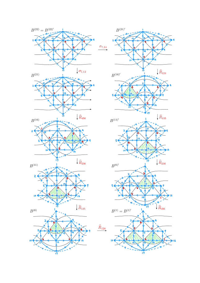
Figure 3.5. Cluster transformations $\widehat{R}_{ijk}$. The wiring diagrams have 6 crossings (red). The quivers (blue) have 17 vertices. Triangles relevant to the image of $\hat{R}_{ijk}$ are hatched in green. The seeds $(B^{(t)},Y^{(t)})$ and $(B^{(t)\prime},Y^{(t)\prime})$ will be explained in detail in Section 3.4.

In Figure 3.5, let $\nu$ and $\nu^{\prime}$ be the mutation sequences corresponding to the left path $(B^{(1)},Y^{(1)})\rightarrow(B^{(6)},Y^{(6)})\rightarrow(B^{(11)},Y^{(11)})\rightarrow(B^{(16)},Y^{(16)})\rightarrow(B^{(22)},Y^{(22)})=\nu(B^{(1)},Y^{(1)})$ and the right path $(B^{(1)\prime},Y^{(1)\prime})\rightarrow(B^{(6)\prime},Y^{(6)\prime})\rightarrow(B^{(11)\prime},Y^{(11)\prime})\rightarrow(B^{(16)\prime},Y^{(16)\prime})\rightarrow(B^{(22)\prime},Y^{(22)\prime})=\nu^{\prime}(B^{(1)},Y^{(1)})$, respectively. Let $\nu(B^{(1)},y^{(1)})$ and $\nu^{\prime}(B^{(1)},y^{(1)})$ be the tropical $y$-seeds generated by the same mutation sequences. It has been checked [20, Sec. A.2] that they satisfy the equality $\nu(B^{(1)},y^{(1)})=\nu^{\prime}(B^{(1)},y^{(1)})$. Thus Theorem 2.4 enforces the equality of quantum $y$-seeds $\nu(B^{(1)},Y^{(1)})=\nu^{\prime}(B^{(1)\prime},Y^{(1)\prime})$. In terms of cluster transformations, it means that the twisted tetrahedron equation $\widehat{R}_{124}\widehat{R}_{135}\widehat{R}_{236}\widehat{R}_{456}\sigma_{7,12}=\widehat{R}_{456}\widehat{R}_{236}\widehat{R}_{135}\widehat{R}_{124}\sigma_{7,14}$ is valid. ∎

3.4. Monomial solutions to the tetrahedron equation

In this subsection we provide additional details regarding Figure 3.5 and Proposition 3.6. Let $(B^{(1)},Y^{(1)})=(B^{(1)\prime},Y^{(1)\prime})$ be the initial quantum $y$-seed corresponding to the quiver at the bottom of Figure 3.5. The quantum $y$-seeds $(B^{(t)},Y^{(t)})$ and $(B^{(t)\prime},Y^{(t)\prime})$ ($t=2$, …, $21$), which pertain to the left and the right paths are determined from it by the mutation sequences, and we have just shown that the final results coincide, i.e., $(B^{(22)},Y^{(22)})=(B^{(22)\prime},Y^{(22)\prime})$. Set $Y^{(t)}=(Y^{(t)}_{1},\dotsc,Y^{(t)}_{17})$ and $Y^{(t)\prime}=(Y^{(t)\prime}_{1},\dotsc,Y^{(t)\prime}_{17})$.

The quantum $y$-seeds $(B^{(t)},Y^{(t)})$ ($t=2,\dotsc,21$) are determined from the initial one $(B^{(1)},Y^{(1)})$ by

$$\begin{split}&(B^{(1)},Y^{(1)})\underset{\varepsilon_{1}}{\overset{\mu_{14}}{\longleftrightarrow}}(B^{(2)},Y^{(2)})\underset{\varepsilon_{2}}{\overset{\mu_{13}}{\longleftrightarrow}}(B^{(3)},Y^{(3)})\underset{\varepsilon_{3}}{\overset{\mu_{15}}{\longleftrightarrow}}(B^{(4)},Y^{(4)})\\ &\qquad\qquad\qquad\qquad\qquad\qquad\qquad\qquad\qquad\qquad\qquad\qquad\underset{\varepsilon_{4}}{\overset{\mu_{8}}{\longleftrightarrow}}(B^{(5)},Y^{(5)})\overset{\sigma_{13,15}\sigma_{8,14}}{\longleftrightarrow}(B^{(6)},Y^{(6)}),\\ &(B^{(6)},Y^{(6)})\underset{\varepsilon_{1}}{\overset{\mu_{7}}{\longleftrightarrow}}(B^{(7)},Y^{(7)})\underset{\varepsilon_{2}}{\overset{\mu_{6}}{\longleftrightarrow}}(B^{(8)},Y^{(8)})\underset{\varepsilon_{3}}{\overset{\mu_{15}}{\longleftrightarrow}}(B^{(9)},Y^{(9)})\\ &\qquad\qquad\qquad\qquad\qquad\qquad\qquad\qquad\qquad\qquad\qquad\qquad\underset{\varepsilon_{4}}{\overset{\mu_{3}}{\longleftrightarrow}}(B^{(10)},Y^{(10)})\overset{\sigma_{6,15}\sigma_{3,7}}{\longleftrightarrow}(B^{(11)},Y^{(11)}),\\ &(B^{(11)},Y^{(11)})\underset{\varepsilon_{1}}{\overset{\mu_{12}}{\longleftrightarrow}}(B^{(12)},Y^{(12)})\underset{\varepsilon_{2}}{\overset{\mu_{11}}{\longleftrightarrow}}(B^{(13)},Y^{(13)})\underset{\varepsilon_{3}}{\overset{\color[rgb]{1,0,0}\mu_{8}}{\longleftrightarrow}}(B^{(14)},Y^{(14)})\\ &\qquad\qquad\qquad\qquad\qquad\qquad\qquad\qquad\qquad\qquad\qquad\qquad\underset{\varepsilon_{4}}{\overset{\mu_{3}}{\longleftrightarrow}}(B^{(15)},Y^{(15)})\overset{\sigma_{8,11}\sigma_{3,12}}{\longleftrightarrow}(B^{(16)},Y^{(16)}),\\ &(B^{(16)},Y^{(16)})\underset{\varepsilon_{1}}{\overset{\color[rgb]{1,0,0}\mu_{14}}{\longleftrightarrow}}(B^{(17)},Y^{(17)})\underset{\varepsilon_{2}}{\overset{\mu_{11}}{\longleftrightarrow}}(B^{(18)},Y^{(18)})\underset{\varepsilon_{3}}{\overset{\mu_{13}}{\longleftrightarrow}}(B^{(19)},Y^{(19)})\\ &\qquad\qquad\qquad\qquad\qquad\qquad\qquad\qquad\qquad\qquad\qquad\qquad\underset{\varepsilon_{4}}{\overset{\mu_{6}}{\longleftrightarrow}}(B^{(20)},Y^{(20)})\overset{\sigma_{11,13}\sigma_{6,14}}{\longleftrightarrow}(B^{(21)},Y^{(21)}),\\ &(B^{(21)},Y^{(21)})\overset{\sigma_{7,12}}{\longleftrightarrow}(B^{(22)},Y^{(22)}),\end{split}$$ (3.20)

where the notation is parallel with (3.3). In particular the choice of signs $\varepsilon_{1}$, …, $\varepsilon_{4}$ does not influence the mutations themselves. According to (3.4), each line in the above corresponds to a cluster transformation appearing in the left path of Figure 3.5 as follows:

$$\begin{split}\widehat{R}_{124}&=\mathrm{Ad}\bigl{(}\Psi_{q}((Y^{(1)}_{14})^{\varepsilon_{1}})^{\varepsilon_{1}}\bigr{)}\tau_{14,\varepsilon_{1}}\mathrm{Ad}\bigl{(}\Psi_{q}((Y^{(2)}_{13})^{\varepsilon_{2}})^{\varepsilon_{2}}\bigr{)}\tau_{13,\varepsilon_{2}}\\ &\quad\times\mathrm{Ad}\bigl{(}\Psi_{q}((Y^{(3)}_{15})^{\varepsilon_{3}})^{\varepsilon_{3}}\bigr{)}\tau_{15,\varepsilon_{3}}\mathrm{Ad}\bigl{(}\Psi_{q}((Y^{(4)}_{8})^{\varepsilon_{4}})^{\varepsilon_{4}}\bigr{)}\tau_{8,\varepsilon_{4}}\sigma_{13,15}\sigma_{8,14},\\ \widehat{R}_{135}&=\mathrm{Ad}\bigl{(}\Psi_{q}((Y^{(6)}_{7})^{\varepsilon_{1}})^{\varepsilon_{1}}\bigr{)}\tau_{7,\varepsilon_{1}}\mathrm{Ad}\bigl{(}\Psi_{q}((Y^{(7)}_{6})^{\varepsilon_{2}})^{\varepsilon_{2}}\bigr{)}\tau_{6,\varepsilon_{2}}\\ &\quad\times\mathrm{Ad}\bigl{(}\Psi_{q}((Y^{(8)}_{15})^{\varepsilon_{3}})^{\varepsilon_{3}}\bigr{)}\tau_{15,\varepsilon_{3}}\mathrm{Ad}\bigl{(}\Psi_{q}((Y^{(9)}_{3})^{\varepsilon_{4}})^{\varepsilon_{4}}\bigr{)}\tau_{3,\varepsilon_{4}}\sigma_{6,15}\sigma_{3,7},\\ \widehat{R}_{236}&=\mathrm{Ad}\bigl{(}\Psi_{q}((Y^{(11)}_{12})^{\varepsilon_{1}})^{\varepsilon_{1}}\bigr{)}\tau_{12,\varepsilon_{1}}\mathrm{Ad}\bigl{(}\Psi_{q}((Y^{(12)}_{11})^{\varepsilon_{2}})^{\varepsilon_{2}}\bigr{)}\tau_{11,\varepsilon_{2}}\\ &\quad\times\mathrm{Ad}\bigl{(}\Psi_{q}((Y^{(13)}_{8})^{\varepsilon_{3}})^{\varepsilon_{3}}\bigr{)}\tau_{8,\varepsilon_{3}}\mathrm{Ad}\bigl{(}\Psi_{q}((Y^{(14)}_{3})^{\varepsilon_{4}})^{\varepsilon_{4}}\bigr{)}\tau_{3,\varepsilon_{4}}\sigma_{8,11}\sigma_{3,12},\\ \widehat{R}_{456}&=\mathrm{Ad}\bigl{(}\Psi_{q}((Y^{(16)}_{14})^{\varepsilon_{1}})^{\varepsilon_{1}}\bigr{)}\tau_{14,\varepsilon_{1}}\mathrm{Ad}\bigl{(}\Psi_{q}((Y^{(17)}_{11})^{\varepsilon_{2}})^{\varepsilon_{2}}\bigr{)}\tau_{11,\varepsilon_{2}}\\ &\quad\times\mathrm{Ad}\bigl{(}\Psi_{q}((Y^{(18)}_{13})^{\varepsilon_{3}})^{\varepsilon_{3}}\bigr{)}\tau_{13,\varepsilon_{3}}\mathrm{Ad}\bigl{(}\Psi_{q}((Y^{(19)}_{6})^{\varepsilon_{4}})^{\varepsilon_{4}}\bigr{)}\tau_{6,\varepsilon_{4}}\sigma_{11,13}\sigma_{6,14}.\end{split}$$ (3.21)

The quantum $y$-seeds $(B^{(t)\prime},Y^{(t)\prime})$ ($t=2$, …, $21$) are determined from the initial one $(B^{(1)\prime},Y^{(1)\prime})$ by

$$\begin{split}&(B^{(1)\prime},Y^{(1)\prime})\underset{\varepsilon_{1}}{\overset{\mu_{12}}{\longleftrightarrow}}(B^{(2)\prime},Y^{(2)\prime})\underset{\varepsilon_{2}}{\overset{\mu_{11}}{\longleftrightarrow}}(B^{(3)\prime},Y^{(3)\prime})\underset{\varepsilon_{3}}{\overset{\mu_{13}}{\longleftrightarrow}}(B^{(4)\prime},Y^{(4)\prime})\\ &\qquad\qquad\qquad\qquad\qquad\qquad\qquad\qquad\qquad\qquad\qquad\qquad\underset{\varepsilon_{4}}{\overset{\mu_{6}}{\longleftrightarrow}}(B^{(5)\prime},Y^{(5)\prime})\overset{\sigma_{11,13}\sigma_{6,12}}{\longleftrightarrow}(B^{(6)\prime},Y^{(6)\prime}),\\ &(B^{(6)\prime},Y^{(6)\prime})\underset{\varepsilon_{1}}{\overset{\mu_{7}}{\longleftrightarrow}}(B^{(7)\prime},Y^{(7)\prime})\underset{\varepsilon_{2}}{\overset{\mu_{11}}{\longleftrightarrow}}(B^{(8)\prime},Y^{(8)\prime})\underset{\varepsilon_{3}}{\overset{\mu_{8}}{\longleftrightarrow}}(B^{(9)\prime},Y^{(9)\prime})\\ &\qquad\qquad\qquad\qquad\qquad\qquad\qquad\qquad\qquad\qquad\qquad\qquad\underset{\varepsilon_{4}}{\overset{\mu_{3}}{\longleftrightarrow}}(B^{(10)\prime},Y^{(10)\prime})\overset{\sigma_{8,11}\sigma_{3,7}}{\longleftrightarrow}(B^{(11)\prime},Y^{(11)\prime}),\\ &(B^{(11)\prime},Y^{(11)\prime})\underset{\varepsilon_{1}}{\overset{\mu_{14}}{\longleftrightarrow}}(B^{(12)\prime},Y^{(12)\prime})\underset{\varepsilon_{2}}{\overset{\color[rgb]{1,0,0}\mu_{6}}{\longleftrightarrow}}(B^{(13)\prime},Y^{(13)\prime})\underset{\varepsilon_{3}}{\overset{\mu_{15}}{\longleftrightarrow}}(B^{(14)\prime},Y^{(14)\prime})\\ &\qquad\qquad\qquad\qquad\qquad\qquad\qquad\qquad\qquad\qquad\qquad\qquad\underset{\varepsilon_{4}}{\overset{\mu_{3}}{\longleftrightarrow}}(B^{(15)\prime},Y^{(15)\prime})\overset{\sigma_{6,15}\sigma_{3,14}}{\longleftrightarrow}(B^{(16)\prime},Y^{(16)\prime}),\\ &(B^{(16)\prime},Y^{(16)\prime})\underset{\varepsilon_{1}}{\overset{\color[rgb]{1,0,0}\mu_{12}}{\longleftrightarrow}}(B^{(17)\prime},Y^{(17)\prime})\underset{\varepsilon_{2}}{\overset{\mu_{13}}{\longleftrightarrow}}(B^{(18)\prime},Y^{(18)\prime})\underset{\varepsilon_{3}}{\overset{\mu_{15}}{\longleftrightarrow}}(B^{(19)\prime},Y^{(19)\prime})\\ &\qquad\qquad\qquad\qquad\qquad\qquad\qquad\qquad\qquad\qquad\qquad\qquad\underset{\varepsilon_{4}}{\overset{\mu_{8}}{\longleftrightarrow}}(B^{(20)\prime},Y^{(20)\prime})\overset{\sigma_{13,15}\sigma_{8,12}}{\longleftrightarrow}(B^{(21)\prime},Y^{(21)\prime}),\\ &(B^{(21)\prime},Y^{(21)\prime})\overset{\sigma_{7,14}}{\longleftrightarrow}(B^{(22)\prime},Y^{(22)\prime}).\end{split}$$ (3.22)

They correspond to the cluster transformations in the right path of Figure 3.5 as follows:

$$\begin{split}\widehat{R}_{456}&=\mathrm{Ad}\bigl{(}\Psi_{q}((Y^{(1)\prime}_{12})^{\varepsilon_{1}})^{\varepsilon_{1}}\bigr{)}\tau_{12,\varepsilon_{1}}\mathrm{Ad}\bigl{(}\Psi_{q}((Y^{(2)\prime}_{11})^{\varepsilon_{2}})^{\varepsilon_{2}}\bigr{)}\tau_{11,\varepsilon_{2}}\\ &\quad\times\mathrm{Ad}\bigl{(}\Psi_{q}((Y^{(3)\prime}_{13})^{\varepsilon_{3}})^{\varepsilon_{z}3}\bigr{)}\tau_{13,\varepsilon_{3}}\mathrm{Ad}\bigl{(}\Psi_{q}((Y^{(4)\prime}_{6})^{\varepsilon_{4}})^{\varepsilon_{4}}\bigr{)}\tau_{6,\varepsilon_{4}}\sigma_{11,13}\sigma_{6,12},\\ \widehat{R}_{236}&=\mathrm{Ad}\bigl{(}\Psi_{q}((Y^{(6)\prime}_{7})^{\varepsilon_{1}})^{\varepsilon_{1}}\bigr{)}\tau_{7,\varepsilon_{1}}\mathrm{Ad}\bigl{(}\Psi_{q}((Y^{(7)\prime}_{11})^{\varepsilon_{2}})^{\varepsilon_{2}}\bigr{)}\tau_{11,\varepsilon_{2}}\\ &\quad\times\mathrm{Ad}\bigl{(}\Psi_{q}((Y^{(8)\prime}_{8})^{\varepsilon_{3}})^{\varepsilon_{3}}\bigr{)}\tau_{8,\varepsilon_{3}}\mathrm{Ad}\bigl{(}\Psi_{q}((Y^{(9)\prime}_{3})^{\varepsilon_{4}})^{\varepsilon_{4}}\bigr{)}\tau_{3,\varepsilon_{4}}\sigma_{8,11}\sigma_{3,7},\\ \widehat{R}_{135}&=\mathrm{Ad}\bigl{(}\Psi_{q}((Y^{(11)\prime}_{14})^{\varepsilon_{1}})^{\varepsilon_{1}}\bigr{)}\tau_{14,\varepsilon_{1}}\mathrm{Ad}\bigl{(}\Psi_{q}((Y^{(12)\prime}_{6})^{\varepsilon_{2}})^{\varepsilon_{2}}\bigr{)}\tau_{6,\varepsilon_{2}}\\ &\quad\times\mathrm{Ad}\bigl{(}\Psi_{q}((Y^{(13)\prime}_{15})^{\varepsilon_{3}})^{\varepsilon_{3}}\bigr{)}\tau_{15,\varepsilon_{3}}\mathrm{Ad}\bigl{(}\Psi_{q}((Y^{(14)\prime}_{3})^{\varepsilon_{4}})^{\varepsilon_{4}}\bigr{)}\tau_{3,\varepsilon_{4}}\sigma_{6,15}\sigma_{3,14},\\ \widehat{R}_{124}&=\mathrm{Ad}\bigl{(}\Psi_{q}((Y^{(16)\prime}_{12})^{\varepsilon_{1}})^{\varepsilon_{1}}\bigr{)}\tau_{12,\varepsilon_{1}}\mathrm{Ad}\bigl{(}\Psi_{q}((Y^{(17)\prime}_{13})^{\varepsilon_{2}})^{\varepsilon_{2}}\bigr{)}\tau_{13,\varepsilon_{2}}\\ &\quad\times\mathrm{Ad}\bigl{(}\Psi_{q}((Y^{(18)\prime}_{15})^{\varepsilon_{3}})^{\varepsilon_{3}}\bigr{)}\tau_{15,\varepsilon_{3}}\mathrm{Ad}\bigl{(}\Psi_{q}((Y^{(19)\prime}_{8})^{\varepsilon_{4}})^{\varepsilon_{4}}\bigr{)}\tau_{8,\varepsilon_{4}}\sigma_{13,15}\sigma_{8,12}.\end{split}$$ (3.23)

Although the formulas (3.21) and (3.23) may appear distinct, they all signify the same transformation described in Proposition 3.4 for the corresponding subsets of $Y$-variables. This fact justifies denoting them by the common symbol $\widehat{R}$.

Remark 3.7.

Consider the tropical $y$-seeds generated by the same mutation sequences from the initial one $(B^{(1)},y^{(1)})=(B^{(1)\prime},y^{(1)\prime})$. Suppose $y^{(1)}_{i}=y^{(1)\prime}_{i}$ is positive for all $i=1$, …, $16$. Then the four mutations highlighted in red in (3.20) and (3.22) are associated to a negative tropical sign of the $y$-variable at the mutation point (the $y$-seed in the left), while the remaining ones are positive.

Let us introduce the monomial parts of the cluster transformations (3.21) and (3.23):

$$\tau_{124|\,\varepsilon_{1},\varepsilon_{2},\varepsilon_{3},\varepsilon_{4}} :=\tau_{14,\varepsilon_{1}}\tau_{13,\varepsilon_{2}}\tau_{15,\varepsilon_{3}}\tau_{8,\varepsilon_{4}}\sigma_{13,15}\sigma_{8,14}:\quad \mathcal{Y}(B^{(6)}) \rightarrow\mathcal{Y}(B^{(1)}),$$

$$\tau_{135|\,\varepsilon_{1},\varepsilon_{2},\varepsilon_{3},\varepsilon_{4}} :=\tau_{7,\varepsilon_{1}}\tau_{6,\varepsilon_{2}}\tau_{15,\varepsilon_{3}}\tau_{3,\varepsilon_{4}}\sigma_{6,15}\sigma_{3,7}: \mathcal{Y}(B^{(11)}) \rightarrow\mathcal{Y}(B^{(6)}),$$

$$\tau_{236|\,\varepsilon_{1},\varepsilon_{2},\varepsilon_{3},\varepsilon_{4}} :=\tau_{12,\varepsilon_{1}}\tau_{11,\varepsilon_{2}}\tau_{8,\varepsilon_{3}}\tau_{3,\varepsilon_{4}}\sigma_{8,11}\sigma_{3,12}: \mathcal{Y}(B^{(16)}) \rightarrow\mathcal{Y}(B^{(11)}),$$

$$\tau_{456|\,\varepsilon_{1},\varepsilon_{2},\varepsilon_{3},\varepsilon_{4}} :=\tau_{14,\varepsilon_{1}}\tau_{11,\varepsilon_{2}}\tau_{13,\varepsilon_{3}}\tau_{6,\varepsilon_{4}}\sigma_{11,13}\sigma_{6,14}: \mathcal{Y}(B^{(21)}) \rightarrow\mathcal{Y}(B^{(16)}),$$

$$\tau^{\prime}_{456|\,\varepsilon_{1},\varepsilon_{2},\varepsilon_{3},\varepsilon_{4}} :=\tau_{12,\varepsilon_{1}}\tau_{11,\varepsilon_{2}}\tau_{13,\varepsilon_{3}}\tau_{6,\varepsilon_{4}}\sigma_{11,13}\sigma_{6,12}:\quad \mathcal{Y}(B^{(6)\prime}) \rightarrow\mathcal{Y}(B^{(1)\prime}),$$

$$\tau^{\prime}_{236|\,\varepsilon_{1},\varepsilon_{2},\varepsilon_{3},\varepsilon_{4}} :=\tau_{7,\varepsilon_{1}}\tau_{11,\varepsilon_{2}}\tau_{8,\varepsilon_{3}}\tau_{3,\varepsilon_{4}}\sigma_{8,11}\sigma_{3,7}:\quad \mathcal{Y}(B^{(11)\prime}) \rightarrow\mathcal{Y}(B^{(6)\prime}),$$

$$\tau^{\prime}_{135|\,\varepsilon_{1},\varepsilon_{2},\varepsilon_{3},\varepsilon_{4}} :=\tau_{14,\varepsilon_{1}}\tau_{6,\varepsilon_{2}}\tau_{15,\varepsilon_{3}}\tau_{3,\varepsilon_{4}}\sigma_{6,15}\sigma_{3,14}:\quad \mathcal{Y}(B^{(16)\prime}) \rightarrow\mathcal{Y}(B^{(11)\prime}),$$

$$\tau^{\prime}_{124|\,\varepsilon_{1},\varepsilon_{2},\varepsilon_{3},\varepsilon_{4}} :=\tau_{12,\varepsilon_{1}}\tau_{13,\varepsilon_{2}}\tau_{15,\varepsilon_{3}}\tau_{8,\varepsilon_{4}}\sigma_{13,15}\sigma_{8,12}:\quad \mathcal{Y}(B^{(21)\prime}) \rightarrow\mathcal{Y}(B^{(16)\prime}).$$

The primes in $\tau^{\prime}_{ijk|\,\varepsilon_{1},\varepsilon_{2},\varepsilon_{3},\varepsilon_{4}}$ are added just for distinction. The maps $\tau_{ijk|\,\varepsilon_{1},\varepsilon_{2},\varepsilon_{3},\varepsilon_{4}}$ and $\tau^{\prime}_{ijk|\,\varepsilon_{1},\varepsilon_{2},\varepsilon_{3},\varepsilon_{4}}$ consistently adhere to $\tau_{\varepsilon_{1},\varepsilon_{2},\varepsilon_{3},\varepsilon_{4}}$ in (3.5) with respect to the subset of $Y$-variables.

Now we are ready to explain monomial solutions to the twisted tetrahedron equation. Proposition 3.6, Figure 3.5 and Remark 2.3 indicate the equality of the tropical $y$-variables $y^{(22)}=y^{(22)\prime}$ provided that all the signs associated with the monomial part of the mutation are chosen to be the tropical signs. Considering Remark 3.7 alongside, we find that

$$\tau_{124|\,++++}\tau_{135|\,++++}\tau_{236|\,++-+}\tau_{456|\,-+++}\sigma_{7,12}=\tau^{\prime}_{456|\,++++}\tau^{\prime}_{236|\,++++}\tau^{\prime}_{135|\,+-++}\tau^{\prime}_{124|\,-+++}\sigma_{7,14}$$ (3.24)

is valid instead of the naive choice of $\tau_{ijk|\,++++}$ and $\tau^{\prime}_{ijk|\,++++}$ everywhere. This is an inhomogeneous version of the twisted tetrahedron equation, as the maps involved are not always uniform in their sign indices. The coincident image of $Y^{(22)}_{1}$, …, $Y^{(22)}_{17}$ by the two sides are sign coherent monomials in the initial $Y$-variables $Y^{(1)}=(Y_{1},\dotsc,Y_{17})$. Their explicit form is available in (A.1).

A natural question is whether there are monomial solutions to the twisted tetrahedron equation with the signs homogeneously chosen as $(\varepsilon_{1},\varepsilon_{2},\varepsilon_{3},\varepsilon_{4})$:

$$\begin{split}&\tau_{124|\,\varepsilon_{1},\varepsilon_{2},\varepsilon_{3},\varepsilon_{4}}\tau_{135|\,\varepsilon_{1},\varepsilon_{2},\varepsilon_{3},\varepsilon_{4}}\tau_{236|\,\varepsilon_{1},\varepsilon_{2},\varepsilon_{3},\varepsilon_{4}}\tau_{456|\,\varepsilon_{1},\varepsilon_{2},\varepsilon_{3},\varepsilon_{4}}\sigma_{7,12}\\ &=\tau^{\prime}_{456|\,\varepsilon_{1},\varepsilon_{2},\varepsilon_{3},\varepsilon_{4}}\tau^{\prime}_{236|\,\varepsilon_{1},\varepsilon_{2},\varepsilon_{3},\varepsilon_{4}}\tau^{\prime}_{135|\,\varepsilon_{1},\varepsilon_{2},\varepsilon_{3},\varepsilon_{4}}\tau^{\prime}_{124|\,\varepsilon_{1},\varepsilon_{2},\varepsilon_{3},\varepsilon_{4}}\sigma_{7,14}.\end{split}$$ (3.25)

The answer is given by a direct calculation as follows.

Proposition 3.8.

The monomial part satisfies the tetrahedron equation (3.25) if and only if $\varepsilon_{1}=-\varepsilon_{4}=-$, i.e., $(\varepsilon_{1},\varepsilon_{2},\varepsilon_{3},\varepsilon_{4})\in\{(-,+,+,+),(-,+,-,+),(-,-,+,+),(-,-,-,+)\}$.

Examples 3.2 and 3.3 describe the monomial parts $\tau_{--++}$ and $\tau_{-+-+}$ explicitly. Analogous information is supplied for the remaining two cases in Appendix A.

3.5. Dilogarithm identities

Now we turn to the dilogarithm identities that will be utilized later. Substitute (3.21) and (3.23) into the LHS and the RHS of (3.19) respectively. The result takes the form

$$\begin{split}&\mathrm{Ad}\bigl{(}\Psi_{q}(U_{1})^{\varepsilon_{1}}\dotsm\Psi_{q}(U_{4})^{\varepsilon_{4}}\bigr{)}\tau_{124|\varepsilon_{1},\varepsilon_{2},\varepsilon_{3},\varepsilon_{4}}\mathrm{Ad}\bigl{(}\Psi_{q}(U_{5})^{\varepsilon_{1}}\dotsm\Psi_{q}(U_{8})^{\varepsilon_{4}}\bigr{)}\tau_{135|\varepsilon_{1},\varepsilon_{2},\varepsilon_{3},\varepsilon_{4}}\\ &\times\mathrm{Ad}\bigl{(}\Psi_{q}(U_{9})^{\varepsilon_{1}}\dotsm\Psi_{q}(U_{12})^{\varepsilon_{4}}\bigr{)}\tau_{236|\varepsilon_{1},\varepsilon_{2},\varepsilon_{3},\varepsilon_{4}}\mathrm{Ad}\bigl{(}\Psi_{q}(U_{13})^{\varepsilon_{1}}\dotsm\Psi_{q}(U_{16})^{\varepsilon_{4}}\bigr{)}\tau_{456|\varepsilon_{1},\varepsilon_{2},\varepsilon_{3},\varepsilon_{4}}\sigma_{7,12}\\ &=\mathrm{Ad}\bigl{(}\Psi_{q}(U^{\prime}_{1})^{\varepsilon_{1}}\dotsm\Psi_{q}(U^{\prime}_{4})^{\varepsilon_{4}}\bigr{)}\tau^{\prime}_{456|\varepsilon_{1},\varepsilon_{2},\varepsilon_{3},\varepsilon_{4}}\mathrm{Ad}\bigl{(}\Psi_{q}(U^{\prime}_{5})^{\varepsilon_{1}}\dotsm\Psi_{q}(U^{\prime}_{8})^{\varepsilon_{4}}\bigr{)}\tau^{\prime}_{236|\varepsilon_{1},\varepsilon_{2},\varepsilon_{3},\varepsilon_{4}}\\ &\quad\times\mathrm{Ad}\bigl{(}\Psi_{q}(U^{\prime}_{9})^{\varepsilon_{1}}\dotsm\Psi_{q}(U^{\prime}_{12})^{\varepsilon_{4}}\bigr{)}\tau^{\prime}_{135|\varepsilon_{1},\varepsilon_{2},\varepsilon_{3},\varepsilon_{4}}\mathrm{Ad}\bigl{(}\Psi_{q}(U^{\prime}_{13})^{\varepsilon_{1}}\dotsm\Psi_{q}(U^{\prime}_{16})^{\varepsilon_{4}}\bigr{)}\tau^{\prime}_{124|\varepsilon_{1},\varepsilon_{2},\varepsilon_{3},\varepsilon_{4}}\sigma_{7,14},\end{split}$$ (3.26)

where $U_{t}$ and $U^{\prime}_{t}$ ($t=1$, …, $16$) denote the $Y$-variables depending on $(\varepsilon_{1},\varepsilon_{2},\varepsilon_{3},\varepsilon_{4})$. Pushing the monomial parts to the right brings (3.26) into the form

$$\begin{split}&\mathrm{Ad}\bigl{(}\Psi_{q}(Z_{1})^{\varepsilon_{1}}\dotsm\Psi_{q}(Z_{16})^{\varepsilon_{4}}\bigr{)}\tau_{124|\varepsilon_{1},\varepsilon_{2},\varepsilon_{3},\varepsilon_{4}}\tau_{135|\varepsilon_{1},\varepsilon_{2},\varepsilon_{3},\varepsilon_{4}}\tau_{236|\varepsilon_{1},\varepsilon_{2},\varepsilon_{3},\varepsilon_{4}}\tau_{456|\varepsilon_{1},\varepsilon_{2},\varepsilon_{3},\varepsilon_{4}}\sigma_{7,12}\\ &=\mathrm{Ad}\bigl{(}\Psi_{q}(Z^{\prime}_{1})^{\varepsilon_{1}}\dotsm\Psi_{q}(Z^{\prime}_{16})^{\varepsilon_{4}}\bigr{)}\tau^{\prime}_{456|\varepsilon_{1},\varepsilon_{2},\varepsilon_{3},\varepsilon_{4}}\tau^{\prime}_{236|\varepsilon_{1},\varepsilon_{2},\varepsilon_{3},\varepsilon_{4}}\tau^{\prime}_{135|\varepsilon_{1},\varepsilon_{2},\varepsilon_{3},\varepsilon_{4}}\tau^{\prime}_{124|\varepsilon_{1},\varepsilon_{2},\varepsilon_{3},\varepsilon_{4}}\sigma_{7,14},\end{split}$$ (3.27)

where $Z_{i}$ and $Z^{\prime}_{i}$ are monomials of $Y_{1}$, …, $Y_{16}$ determined by

$$Z_{i}=\begin{cases}U_{i}&(i=1,\dotsc,4),\\ \tau_{124|\varepsilon_{1},\varepsilon_{2},\varepsilon_{3},\varepsilon_{4}}(U_{i})&(i=5,\dotsc,8),\\ \tau_{124|\varepsilon_{1},\varepsilon_{2},\varepsilon_{3},\varepsilon_{4}}\tau_{135|\varepsilon_{1},\varepsilon_{2},\varepsilon_{3},\varepsilon_{4}}(U_{i})&(i=9,\ldots,12),\\ \tau_{124|\varepsilon_{1},\varepsilon_{2},\varepsilon_{3},\varepsilon_{4}}\tau_{135|\varepsilon_{1},\varepsilon_{2},\varepsilon_{3},\varepsilon_{4}}\tau_{236|\varepsilon_{1},\varepsilon_{2},\varepsilon_{3},\varepsilon_{4}}(U_{i})&(i=13,\ldots,16).\end{cases}$$ (3.28)

The elements $Z^{\prime}_{i}$ are similarly determined from the RHS of (3.26). From (3.27) and Proposition 3.8 we deduce

$$\mathrm{Ad}\bigl{(}\Psi_{q}(Z_{1})^{\varepsilon_{1}}\cdots\Psi_{q}(Z_{16})^{\varepsilon_{4}}\bigr{)}=\mathrm{Ad}\bigl{(}\Psi_{q}(Z^{\prime}_{1})^{\varepsilon_{1}}\cdots\Psi_{q}(Z^{\prime}_{16})^{\varepsilon_{4}}\bigr{)}$$ (3.29)

for $(\varepsilon_{1},\varepsilon_{2},\varepsilon_{3},\varepsilon_{4})\in\{(-,+,+,+),(-,+,-,+),(-,-,+,+),(-,-,-,+)\}$. Actually a stronger equality holds.

Proposition 3.9.

For $(\varepsilon_{1},\varepsilon_{2},\varepsilon_{3},\varepsilon_{4})\in\{(-,+,-,+),(-,-,+,+)\}$, the products of quantum dilogarithms within $\mathrm{Ad}$ in (3.29) are well-defined formal Laurent series in the nine $Y$-variables $Y_{3}$, $Y_{6}$, $Y_{7}$, $Y_{8}$, $Y_{11}$, $Y_{12}$, $Y_{13}$, $Y_{14}$ and $Y_{15}$. Moreover they are equal, i.e.,

$$\Psi_{q}(Z_{1})^{\varepsilon_{1}}\dotsm\Psi_{q}(Z_{16})^{\varepsilon_{4}}=\Psi_{q}(Z^{\prime}_{1})^{\varepsilon_{1}}\dotsm\Psi_{q}(Z^{\prime}_{16})^{\varepsilon_{4}}.$$ (3.30)

Proof.

We show the claim for $(\varepsilon_{1},\varepsilon_{2},\varepsilon_{3},\varepsilon_{4})=(-,-,+,+)$. The case $(-,+,-,+)$ is similar. The data $Z_{1}$, …, $Z_{16}$ for $(\varepsilon_{1},\varepsilon_{2},\varepsilon_{3},\varepsilon_{4})=(-,-,+,+)$ is given by

$$\begin{pmatrix}Y_{14}^{-1}&qY^{-1}_{13}Y^{-1}_{14}&q^{-1}Y_{14}Y_{15}&q^{-2}Y_{8}Y_{14}Y_{15}\\ q^{2}Y^{-1}_{7}Y^{-1}_{13}Y^{-1}_{14}&q^{3}Y^{-1}_{6}Y^{-1}_{7}Y^{-1}_{13}Y^{-1}_{14}&q^{-3}Y_{7}Y_{8}Y_{14}Y_{15}&q^{-4}Y_{3}Y_{7}Y_{8}Y_{14}Y_{15}\\ Y^{-1}_{12}&qY^{-1}_{11}Y^{-1}_{12}&q^{-1}Y_{12}Y_{13}&q^{-2}Y_{6}Y_{12}Y_{13}\\ Y^{-1}_{7}&qY^{-1}_{6}Y^{-1}_{7}&q^{-1}Y_{7}Y_{8}&q^{-2}Y_{3}Y_{7}Y_{8}\end{pmatrix},$$ (3.31)

where the element at $i$th row and the $j$th column from the top left signifies $Z_{4i+j-4}$. Similarly, the data $Z^{\prime}_{1},\dotsc,Z^{\prime}_{16}$ is given as follows:

$$\begin{pmatrix}Y^{-1}_{12}&qY^{-1}_{11}Y^{-1}_{12}&q^{-1}Y_{12}Y_{13}&q^{-2}Y_{6}Y_{12}Y_{13}\\ Y^{-1}_{7}&qY^{-1}_{6}Y^{-1}_{7}&q^{-1}Y_{7}Y_{8}&q^{-2}Y_{3}Y_{7}Y_{8}\\ Y^{-1}_{12}Y^{-1}_{13}Y^{-1}_{14}&qY^{-1}_{11}Y^{-1}_{12}Y^{-1}_{13}Y^{-1}_{14}&q^{-1}Y_{12}Y_{13}Y_{14}Y_{15}&q^{-2}Y_{6}Y_{12}Y_{13}Y_{14}Y_{15}\\ Y_{6}Y^{-1}_{11}Y^{-1}_{14}&qY^{-1}_{13}Y^{-1}_{14}&q^{-1}Y_{14}Y_{15}&q^{-2}Y_{3}Y^{-1}_{6}Y_{8}Y_{14}Y_{15}\end{pmatrix}.$$ (3.32)

Note that $Z^{\prime}_{13}$ and $Z^{\prime}_{16}$ in (3.31) are not sign coherent. In order to show the well-definedness of the LHS of (3.30), expand the 16 $\Psi_{q}$’s via (2.7) with the summation variables $n_{1}$, …, $n_{16}\in{\mathbb{Z}}_{\geq 0}$. By using the $q$-commutativity of $Y$-variables, one can arrange each term of the expansion uniquely as

$$\begin{split}&\Psi_{q}(Z_{1})^{-1}\Psi_{q}(Z_{2})^{-1}\Psi_{q}(Z_{3})\Psi_{q}(Z_{4})\dotsm\Psi_{q}(Z_{13})^{-1}\Psi_{q}(Z_{14})^{-1}\Psi_{q}(Z_{15})\Psi_{q}(Z_{16})\\ &=\sum_{\mathbf{n}\in({\mathbb{Z}}_{\geq 0})^{16}}C(\mathbf{n})Y_{3}^{p_{1}}Y_{6}^{p_{2}}Y_{7}^{p_{3}}Y_{8}^{p_{4}}Y_{11}^{p_{5}}Y_{12}^{p_{6}}Y_{13}^{p_{7}}Y_{14}^{p_{8}}Y_{15}^{p_{9}},\end{split}$$ (3.33)

where $C(\mathbf{n})$ is a rational function of $q$ depending on $\mathbf{n}=(n_{1},\dotsc,n_{16})$. The powers $p_{i}$’s are given by

$$p_{1} =n_{8}+n_{16}, p_{6} =-n_{9}-n_{10}-n_{11}-n_{13}-n_{15},$$

$$p_{2} =-n_{6}+n_{12}-n_{14}, p_{7} =-n_{2}-n_{5}-n_{6}-n_{11}-n_{13}-n_{15},$$

$$p_{3} =-n_{5}-n_{6}-n_{7}+n_{12}-n_{14}-n_{16},\;\;\; p_{8} =-n_{1}-n_{2}-n_{3}-n_{5}-n_{6}-n_{11}-n_{13},$$

$$p_{4} =n_{4}-n_{7}+n_{12}+n_{13}-n_{16}, p_{9} =-n_{3}-n_{11}-n_{13}.$$

$$p_{5} =-n_{10},$$ (3.34)

The series (3.33) is well-defined if the coefficient of the monomial $Y_{3}^{p_{1}}Y_{6}^{p_{2}}Y_{7}^{p_{3}}Y_{8}^{p_{4}}Y_{11}^{p_{5}}Y_{12}^{p_{6}}Y_{13}^{p_{7}}Y_{14}^{p_{8}}Y_{15}^{p_{9}}$ for any given $(p_{1},\dotsc,p_{9})\in{\mathbb{Z}}^{9}$ is finite. This is shown by checking that there are none or finitely many $\mathbf{n}\in({\mathbb{Z}}_{\geq 0})^{16}$ satisfying the nine equations (3.34). This is straightforward. The well-definedness of the RHS is verified in the same manner.

Next we prove (3.30). From (3.29) we know that $\mathrm{Ad}\bigl{(}(\text{LHS})(\text{RHS})^{-1}\bigr{)}=1$. From an argument similar to the proof of [13, Th. 3.5], it follows that $(\text{LHS})(\text{RHS})^{-1}=c$, where $c$ only depends on $q$. To determine $c$, we compare the constant terms contained in the LHS and the RHS. For the LHS, one looks for $\mathbf{n}\in({\mathbb{Z}}_{\geq 0})^{16}$ such that $p_{1}=\dotsb=p_{9}=0$. It is easy to see that $\mathbf{n}=(0,\dotsc,0)$ is the only solution indicating that the constant term of the LHS is 1. Similarly, the constant term of the RHS is found to be 1. Therefore $c=1$. ∎

Remark 3.10.

For the two cases $(\varepsilon_{1},\varepsilon_{2},\varepsilon_{3},\varepsilon_{4})=(-,+,+,+),(-,-,-,+)$ in Proposition 3.8, there are infinitely many choices of $\mathbf{n}\in({\mathbb{Z}}_{\geq 0})^{16}$ satisfying (3.34). Therefore the simple argument in the above proof is not valid.

4. Realization in terms of $q$-Weyl algebras

4.1. $Y$-variables and $q$-Weyl algebras

Hereafter we also use $\hbar$ which is related to $q$ by $q={\mathrm{e}}^{\hbar}$. By a $q$-Weyl algebra we mean an associative algebra generated by $U^{\pm 1}$ and $W^{\pm 1}$ obeying the relations $UU^{-1}=U^{-1}U=WW^{-1}=W^{-1}W=1$ and $UW=qWU$. To each crossing $i$ of the wiring diagram we associate parameters $\mathscr{P}_{i}=(a_{i},b_{i},c_{i},d_{i},e_{i})$ and canonical variables $u_{i}$, $w_{i}$ satisfying

$$[u_{i},w_{j}]=\hbar\delta_{ij},\quad[u_{i},u_{j}]=[w_{i},w_{j}]=0.$$ (4.1)

$$a_{i}+b_{i}+c_{i}+d_{i}+e_{i}=0.$$ (4.2)

The exponentials of the canonical variables obey the relations in a direct product of $q$-Weyl algebras, e.g., ${\mathrm{e}}^{u_{i}}{\mathrm{e}}^{w_{j}}=q^{\delta_{ij}}{\mathrm{e}}^{w_{j}}{\mathrm{e}}^{u_{i}}$. Given a wiring diagram and the associated symmetric butterfly quiver, we “parameterize” the $Y$-variables by the graphical rule explained in Figure 4.1.

Figure 4.1. Graphical rule to parametrize the $Y$-variables in terms of $q$-Weyl algebra generators in the vicinity of the crossing $i$ (center) of the wiring diagram (black). A $Y$-variable situated at a vertex (blue circle) of the symmetric butterfly quiver acquires factors ${\mathrm{e}}^{a_{i}+w_{i}}$, ${\mathrm{e}}^{b_{i}-u_{i}-w_{i}}$, ${\mathrm{e}}^{c_{i}+w_{i}}$, ${\mathrm{e}}^{d_{i}-u_{i}-w_{i}}$ from the neighboring crossing $i$ of the wiring diagram if the vertex is located at the north, east, south, west of $i$, respectively. A $Y$-variable on the vertex $i$ is ${\mathrm{e}}^{e_{i}+2u_{i}}$. The ordering of these factors from different $i$’s (if any) is inconsequential due to the commutativity of the associated canonical variables.

The claim is that the relation $Y_{r}Y_{s}=q^{2b_{rs}}Y_{s}Y_{r}$ (2.1) is satisfied under this parameterization. To state it formally, let $\mathcal{W}_{n}$ be the direct product of the $q$-Weyl algebras generated by ${\mathrm{e}}^{\pm u_{i}}$, ${\mathrm{e}}^{\pm w_{i}}$ for $i=1$, …, $n$. Let further $\mathcal{A}_{n}$ be the non-commuting fractional field of $\mathcal{W}_{n}$. Then for $B$ corresponding to the left diagram in Figure 3.4, we have a morphism $\phi_{\mathrm{SB}}\colon\mathcal{Y}(B)\rightarrow\mathcal{A}_{3}$ defined by

$$\phi_{\mathrm{SB}}:\begin{cases}Y_{1}\mapsto{\mathrm{e}}^{c_{1}+c_{3}+w_{1}+w_{3}},&Y_{6}\mapsto{\mathrm{e}}^{b_{1}-u_{1}-w_{1}},\\ Y_{2}\mapsto{\mathrm{e}}^{d_{3}-u_{3}-w_{3}},&Y_{7}\mapsto{\mathrm{e}}^{d_{2}+a_{3}-u_{2}-w_{2}+w_{3}},\\ Y_{3}\mapsto{\mathrm{e}}^{e_{3}+2u_{3}},&Y_{8}\mapsto{\mathrm{e}}^{e_{2}+2u_{2}},\\ Y_{4}\mapsto{\mathrm{e}}^{d_{1}+c_{2}+b_{3}-u_{1}-w_{1}+w_{2}-u_{3}-w_{3}},&Y_{9}\mapsto{\mathrm{e}}^{a_{1}+b_{2}+w_{1}-u_{2}-w_{2}},\\ Y_{5}\mapsto{\mathrm{e}}^{e_{1}+2u_{1}},&Y_{10}\mapsto{\mathrm{e}}^{a_{2}+w_{2}},\end{cases}$$ (4.3)

where SB signifies “symmetric butterfly.” Similarly, for the right diagram of Figure 3.4, we have a morphism $\phi^{\prime}_{\mathrm{SB}}\colon\mathcal{Y}(B^{\prime})\rightarrow\mathcal{A}_{3}$ as

$$\phi^{\prime}_{\mathrm{SB}}:\begin{cases}Y^{\prime}_{1}\mapsto{\mathrm{e}}^{c_{2}+w_{2}},&Y^{\prime}_{6}\mapsto{\mathrm{e}}^{b_{2}+c_{3}-u_{2}-w_{2}+w_{3}},\\ Y^{\prime}_{2}\mapsto{\mathrm{e}}^{c_{1}+d_{2}+w_{1}-u_{2}-w_{2}},&Y^{\prime}_{7}\mapsto{\mathrm{e}}^{d_{1}-u_{1}-w_{1}},\\ Y^{\prime}_{3}\mapsto{\mathrm{e}}^{e_{3}+2u_{3}},&Y^{\prime}_{8}\mapsto{\mathrm{e}}^{e_{2}+2u_{2}},\\ Y^{\prime}_{4}\mapsto{\mathrm{e}}^{b_{1}+a_{2}+d_{3}-u_{1}-w_{1}+w_{2}-u_{3}-w_{3}},&Y^{\prime}_{9}\mapsto{\mathrm{e}}^{b_{3}-u_{3}-w_{3}},\\ Y^{\prime}_{5}\mapsto{\mathrm{e}}^{e_{1}+2u_{1}},&Y^{\prime}_{10}\mapsto{\mathrm{e}}^{a_{1}+a_{3}+w_{1}+w_{3}}.\end{cases}$$ (4.4)

Remark 4.1.

In the parameterization (4.3), the centers in Remark 3.1 take the following values:

$$\phi_{\mathrm{SB}}(Y^{-1}_{1}Y_{7}Y_{8}Y_{9}Y^{2}_{10}) ={\mathrm{e}}^{a_{1}-c_{1}+a_{2}-c_{2}+a_{3}-c_{3}},$$ (4.5)

$$\phi_{\mathrm{SB}}(Y_{2}Y^{-1}_{4}Y_{6}Y_{10}) ={\mathrm{e}}^{b_{1}-d_{1}+a_{2}-c_{2}+d_{3}-b_{3}},$$ (4.6)

$$\phi_{\mathrm{SB}}(Y_{3}Y^{2}_{4}Y^{-2}_{6}Y^{2}_{7}Y_{8}) ={\mathrm{e}}^{2d_{1}-2b_{1}+2c_{2}+2d_{2}+e_{2}+2a_{3}+2b_{3}+e_{3}},$$ (4.7)

$$\phi_{\mathrm{SB}}(Y_{5}Y^{2}_{6}Y_{8}Y^{2}_{9}Y^{2}_{10}) =q^{-4}{\mathrm{e}}^{2a_{1}+2b_{1}+e_{1}+2a_{2}+2b_{2}+e_{2}}.$$ (4.8)

In both parameterization (4.3) and (4.4), the invariants in Remark 3.5 take the following forms:

$$\phi_{\mathrm{SB}}(Y_{3}Y_{8})=\phi^{\prime}_{\mathrm{SB}}(Y^{\prime}_{3}Y^{\prime}_{8})={\mathrm{e}}^{e_{2}+e_{3}+u_{2}+u_{3}},$$ (4.9)

$$\phi_{\mathrm{SB}}(Y_{5}Y_{8})=\phi^{\prime}_{\mathrm{SB}}(Y^{\prime}_{5}Y^{\prime}_{8})={\mathrm{e}}^{e_{1}+e_{2}+u_{1}+u_{2}},$$ (4.10)

$$\phi_{\mathrm{SB}}(Y_{1}Y_{2}Y_{4}Y_{6}Y_{7}Y^{-1}_{8}Y_{9}Y_{10})=\phi^{\prime}_{\mathrm{SB}}(Y^{\prime}_{1}Y^{\prime}_{2}Y^{\prime}_{4}Y^{\prime}_{6}Y^{\prime}_{7}Y^{\prime-1}_{8}Y^{\prime}_{9}Y^{\prime}_{10})={\mathrm{e}}^{-e_{1}-2e_{2}-e_{3}-2u_{1}-4u_{2}-2u_{3}}.$$ (4.11)

The combinations $u_{1}+u_{2}$ and $u_{2}+u_{3}$ will reemerge as conserved quantities within the delta functions in the matrix elements of the $R$-matrix in coordinate representations. See (5.10) and (6.15).

4.2. Extracting $R_{123}$ from $\widehat{R}_{123}$

Let us illustrate the action of the monomial part $\tau_{\varepsilon_{1},\varepsilon_{2},\varepsilon_{3},\varepsilon_{4}}$ (3.5) of $\widehat{R}_{123}$ on the canonical variables for the case $(\varepsilon_{1},\varepsilon_{2},\varepsilon_{3},\varepsilon_{4})=(-,-,+,+)$. From Example 3.2 and (4.3)–(4.4), we find that $\tau_{--++}$ is translated into a transformation $\tau^{uw}_{--++}$ of the canonical variables as

$$\tau^{uw}_{--++}:\;\begin{cases}u_{1}\mapsto u_{1}+u_{2}-u_{3}+\lambda_{0},\quad\;\;w_{1}\mapsto w_{1}+\lambda_{1},\\ u_{2}\mapsto u_{3}-\lambda_{0},\qquad\qquad\qquad w_{2}\mapsto w_{1}+w_{3}+\lambda_{3},\\ u_{3}\mapsto u_{2}+\lambda_{0},\qquad\qquad\qquad w_{3}\mapsto-w_{1}+w_{2}+\lambda_{2},\end{cases}$$ (4.12)

where $\lambda_{r}=\lambda_{r}(\mathscr{P}_{1},\mathscr{P}_{2},\mathscr{P}_{3})$ for $r=0$, $1$, $2$, $3$ is defined, under the condition (4.2), by

$$\lambda_{0}=\frac{e_{2}-e_{3}}{2},\quad\lambda_{1}=a_{2}-a_{3}+b_{2}-b_{3}+\lambda_{0},\quad\lambda_{2}=-a_{1}-b_{2}+b_{3}-\lambda_{0},\quad\lambda_{3}=c_{1}-c_{2}+c_{3}.$$ (4.13)

In order to realize (4.12) as an adjoint action, we introduce the group $N_{n}$ generated by

$${\mathrm{e}}^{\pm\tfrac{1}{\hbar}u_{i}w_{j}}\ (i\neq j),\quad{\mathrm{e}}^{\tfrac{a}{\hbar}u_{i}},\ {\mathrm{e}}^{\tfrac{a}{\hbar}w_{i}}\ (a\in{\mathbb{C}}),\quad b\in{\mathbb{C}}^{\times}$$ (4.14)

with $i$, $j\in\{1,\dotsc,n\}$. The multiplication is defined by the (generalized) BCH formula and (4.1), which is well-defined due to the grading by $\hbar^{-1}$. Let $\mathfrak{S}_{n}$ be the symmetric group generated by the transpositions $\rho_{ij}$ ($i$, $j\in\{1,\dotsc,n\}$). It acts on $N_{n}$ via the adjoint action, inducing permutations of the indices of the canonical variables. Thus one can form the semi-direct product $N_{n}\rtimes\mathfrak{S}_{n}$, and let it act on $\mathcal{W}_{n}$ by the adjoint action.

Now the monomial part $\tau^{uw}_{--++}$ is described as the adjoint action as follows:

$$\tau^{uw}_{--++} =\mathrm{Ad}(P_{--++}),$$ (4.15)

$$P_{--++} ={\mathrm{e}}^{\tfrac{1}{\hbar}(u_{3}-u_{2})w_{1}}{\mathrm{e}}^{\tfrac{\lambda_{0}}{\hbar}(-w_{1}-w_{2}+w_{3})}{\mathrm{e}}^{\tfrac{1}{\hbar}(\lambda_{1}u_{1}+\lambda_{2}u_{2}+\lambda_{3}u_{3})}\rho_{23}\in N_{3}\rtimes\mathfrak{S}_{3},$$ (4.16)

where $\rho_{23}$ acts trivially on the parameters $\lambda_{r}$. Extending the indices and suppressing the sign choice of $--++$ in (4.15) and (4.16), we introduce

$$\tau^{uw}_{ijk} =\mathrm{Ad}(P_{ijk}),$$ (4.17)

$$P_{ijk} ={\mathrm{e}}^{\tfrac{1}{\hbar}(u_{k}-u_{j})w_{i}}{\mathrm{e}}^{\tfrac{\lambda_{0}}{\hbar}(-w_{i}-w_{j}+w_{k})}{\mathrm{e}}^{\tfrac{1}{\hbar}(\lambda_{1}u_{i}+\lambda_{2}u_{j}+\lambda_{3}u_{k})}\rho_{jk}\in N_{6}\rtimes\mathfrak{S}_{6},$$ (4.18)

where $\lambda_{r}=\lambda_{r}(\mathscr{P}_{i},\mathscr{P}_{j},\mathscr{P}_{k})$ is given by (4.13) by replacing the parameters as $(\mathscr{P}_{1},\mathscr{P}_{2},\mathscr{P}_{3})\rightarrow(\mathscr{P}_{i},\mathscr{P}_{j},\mathscr{P}_{k})$. By a straightforward calculation using the BCH formula, one can prove

Lemma 4.2.

$P_{ijk}$ satisfies the tetrahedron equation in $N_{6}\rtimes\mathfrak{S}_{6}$ by itself:

$$P_{124}P_{135}P_{236}P_{456}=P_{456}P_{236}P_{135}P_{124}.$$ (4.19)

The fact that $P_{ijk}$ acts on the canonical variables rather than $Y$-variables has led to the tetrahedron equation without a twist by permutations.

Define $R_{123}=R(\mathscr{P}_{1},\mathscr{P}_{2},\mathscr{P}_{3})_{123}$ by

$$R_{123} =\Psi_{q}({\mathrm{e}}^{-d_{1}-c_{2}-b_{3}+u_{1}+u_{3}+w_{1}-w_{2}+w_{3}})^{-1}\Psi_{q}({\mathrm{e}}^{-d_{1}-c_{2}-b_{3}-e_{3}+u_{1}-u_{3}+w_{1}-w_{2}+w_{3}})^{-1}$$

$$\quad\times\Psi_{q}({\mathrm{e}}^{d_{1}+e_{1}+c_{2}+b_{3}+u_{1}-u_{3}-w_{1}+w_{2}-w_{3}})\Psi_{q}({\mathrm{e}}^{d_{1}+e_{1}+c_{2}+e_{2}+b_{3}+u_{1}+2u_{2}-u_{3}-w_{1}+w_{2}-w_{3}})P_{123}$$ (4.20)

$$=\Psi_{q}({\mathrm{e}}^{-d_{1}-c_{2}-b_{3}+u_{1}+u_{3}+w_{1}-w_{2}+w_{3}})^{-1}\Psi_{q}({\mathrm{e}}^{-d_{1}-c_{2}-b_{3}-e_{3}+u_{1}-u_{3}+w_{1}-w_{2}+w_{3}})^{-1}$$

$$\quad\times P_{123}\Psi_{q}({\mathrm{e}}^{-b_{1}-a_{2}-d_{3}-e_{3}+u_{1}-u_{3}+w_{1}-w_{2}+w_{3}})\Psi_{q}({\mathrm{e}}^{-b_{1}-a_{2}-d_{3}+u_{1}+u_{3}+w_{1}-w_{2}+w_{3}}).$$ (4.21)

Let $\widehat{R}^{uw}_{123}$ be the cluster transformation $\widehat{R}_{123}$ (3.9) viewed as the one for the canonical variables $\{u_{i},w_{i}\}_{i=1,2,3}$. Then from (4.3), (4.4) and (4.15), we have

$$\widehat{R}^{uw}_{123} =\mathrm{Ad}\bigl{(}R(\mathscr{P}_{1},\mathscr{P}_{2},\mathscr{P}_{3})_{123}\bigr{)}.$$ (4.22)

Note that the RHS is invariant under $R\rightarrow cR$ for any scalar $c$. A proper normalization of $R$ based on a symmetry consideration will be proposed in Section 4.3.

Formally the results (4.12) and (4.22) may be stated as the commutativity of the diagrams:

$$\begin{CD}\mathcal{Y}(B^{\prime})@>{{\tau_{--++}}}>{}>\mathcal{Y}(B)\\ @V{\phi^{\prime}_{\mathrm{SB}}}V{}V@V{}V{\phi_{\mathrm{SB}}}V\\ \mathcal{A}_{3}@>{\tau^{uw}_{--++}}>{}>\mathcal{A}_{3}\end{CD}\qquad\qquad\begin{CD}\mathcal{Y}(B^{\prime})@>{{\widehat{R}_{123}}}>{}>\mathcal{Y}(B)\\ @V{\phi^{\prime}_{\mathrm{SB}}}V{}V@V{}V{\phi_{\mathrm{SB}}}V\\ \mathcal{A}_{3}@>{\widehat{R}^{uw}_{123}}>{}>\mathcal{A}_{3}\end{CD}$$ (4.23)

Extending (4.20) and (4.21), we introduce $R_{ijk}=R(\mathscr{P}_{i},\mathscr{P}_{j},\mathscr{P}_{k})_{ijk}$ by

$$R_{ijk} =\Psi_{q}({\mathrm{e}}^{-d_{i}-c_{j}-b_{k}+u_{i}+u_{k}+w_{i}-w_{j}+w_{k}})^{-1}\Psi_{q}({\mathrm{e}}^{-d_{i}-c_{j}-b_{k}-e_{k}+u_{i}-u_{k}+w_{i}-w_{j}+w_{k}})^{-1}$$

$$\quad\times\Psi_{q}({\mathrm{e}}^{d_{i}+e_{i}+c_{j}+b_{k}+u_{i}-u_{k}-w_{i}+w_{j}-w_{k}})\Psi_{q}({\mathrm{e}}^{d_{i}+e_{i}+c_{j}+e_{j}+b_{k}+u_{i}+2u_{j}-u_{k}-w_{i}+w_{j}-w_{k}})P_{ijk}$$ (4.24)

$$=\Psi_{q}({\mathrm{e}}^{-d_{i}-c_{j}-b_{k}+u_{i}+u_{k}+w_{i}-w_{j}+w_{k}})^{-1}\Psi_{q}({\mathrm{e}}^{-d_{i}-c_{j}-b_{k}-e_{k}+u_{i}-u_{k}+w_{i}-w_{j}+w_{k}})^{-1}$$

$$\quad\times P_{ijk}\Psi_{q}({\mathrm{e}}^{-b_{i}-a_{j}-d_{k}-e_{k}+u_{i}-u_{k}+w_{i}-w_{j}+w_{k}})\Psi_{q}({\mathrm{e}}^{-b_{i}-a_{j}-d_{k}+u_{i}+u_{k}+w_{i}-w_{j}+w_{k}}),$$ (4.25)

where $P_{ijk}$ is given by (4.18). Now we state the main result of the paper.

Theorem 4.3.

$R(\mathscr{P}_{i},\mathscr{P}_{j},\mathscr{P}_{k})_{ijk}$ satisfies the tetrahedron equation:

$$\begin{split}&\;R(\mathscr{P}_{1},\mathscr{P}_{2},\mathscr{P}_{4})_{124}R(\mathscr{P}_{1},\mathscr{P}_{3},\mathscr{P}_{5})_{135}R(\mathscr{P}_{2},\mathscr{P}_{3},\mathscr{P}_{6})_{236}R(\mathscr{P}_{4},\mathscr{P}_{5},\mathscr{P}_{6})_{456}\\ &\;=R(\mathscr{P}_{4},\mathscr{P}_{5},\mathscr{P}_{6})_{456}R(\mathscr{P}_{2},\mathscr{P}_{3},\mathscr{P}_{6})_{236}R(\mathscr{P}_{1},\mathscr{P}_{3},\mathscr{P}_{5})_{135}R(\mathscr{P}_{1},\mathscr{P}_{2},\mathscr{P}_{4})_{124}.\end{split}$$ (4.26)

Proof.

Consider the dilogarithm identity (3.30) with $(\varepsilon_{1},\varepsilon_{2},\varepsilon_{3},\varepsilon_{4})=(-,-,+,+)$ in terms of canonical variables

$$\Psi_{q}(\tilde{Z}_{1})^{\varepsilon_{1}}\dotsm\Psi_{q}({\tilde{Z}}_{16})^{\varepsilon_{4}}=\Psi_{q}(\tilde{Z^{\prime}}_{1})^{\varepsilon_{1}}\dotsm\Psi_{q}(\tilde{Z^{\prime}}_{16})^{\varepsilon_{4}}.$$ (4.27)

Here $\tilde{Z}_{i}=\tilde{\phi}_{\mathrm{SB}}(Z_{i})$ and $\tilde{Z^{\prime}}_{i}=\tilde{\phi}^{\prime}_{\mathrm{SB}}(Z^{\prime}_{i})$ with $Z_{i}$ and $Z^{\prime}_{i}$ given in (3.31) and (3.32). The morphisms $\tilde{\phi}_{\mathrm{SB}}$ and $\tilde{\phi}^{\prime}_{\mathrm{SB}}$ are natural generalizations of (4.3) and (4.4). They send the $Y$-variables to $\mathcal{W}_{6}$ according to the rule in Figure 4.1 applied to the bottom right diagram in Figure 3.5. Multiplication of (4.19) to (4.27) from the right leads to

$$\Psi_{q}(\tilde{Z}_{1})^{\varepsilon_{1}}\dotsm\Psi_{q}({\tilde{Z}}_{16})^{\varepsilon_{4}}P_{124}P_{135}P_{236}P_{456}=\Psi_{q}(\tilde{Z^{\prime}}_{1})^{\varepsilon_{1}}\dotsm\Psi_{q}(\tilde{Z^{\prime}}_{16})^{\varepsilon_{4}}P_{456}P_{236}P_{135}P_{124}.$$ (4.28)

Let us consider the LHS. It is obviously equal to

$$\begin{split}&\Psi_{q}(\tilde{Z}_{1})^{\varepsilon_{1}}\dotsm\Psi_{q}({\tilde{Z}}_{4})^{\varepsilon_{4}}P_{124}\\ &\times P^{-1}_{124}\Psi_{q}(\tilde{Z}_{5})^{\varepsilon_{1}}\dotsm\Psi_{q}({\tilde{Z}}_{8})^{\varepsilon_{4}}P_{124}\cdot P_{135}\\ &\times P^{-1}_{135}P^{-1}_{124}\Psi_{q}(\tilde{Z}_{9})^{\varepsilon_{1}}\dotsm\Psi_{q}({\tilde{Z}}_{12})^{\varepsilon_{4}}P_{124}P_{135}\cdot P_{236}\\ &\times P^{-1}_{236}P^{-1}_{135}P^{-1}_{124}\Psi_{q}(\tilde{Z}_{13})^{\varepsilon_{1}}\dotsm\Psi_{q}({\tilde{Z}}_{16})^{\varepsilon_{4}}P_{124}P_{135}P_{236}\cdot P_{456}.\end{split}$$ (4.29)

On the other hand from (4.17) and the image of $(\ref{zu})$ by $\tilde{\phi}_{\mathrm{SB}}$, we know

$${\tilde{U}}_{i}=\begin{cases}\tilde{Z}_{i}&(i=1,\dotsc,4),\\ P_{124}^{-1}\tilde{Z}_{i}P_{124}&(i=5,\dotsc,8),\\ P_{135}^{-1}P_{135}^{-1}\tilde{Z}_{i}P_{124}P_{135}&(i=9,\dotsc,12),\\ P_{236}^{-1}P_{135}^{-1}P_{124}^{-1}\tilde{Z}_{i}P_{124}P_{135}P_{236}&(i=13,\dotsc,16).\end{cases}$$ (4.30)

where $\tilde{U}_{i}=\tilde{\phi}_{\mathrm{SB}}(U_{i})$. Thus (4.29) is cast into the form

$$\begin{split}&\Psi_{q}(\tilde{U}_{1})^{\varepsilon_{1}}\cdots\Psi_{q}({\tilde{U}}_{4})^{\varepsilon_{4}}P_{124}\Psi_{q}(\tilde{U}_{5})^{\varepsilon_{1}}\cdots\Psi_{q}({\tilde{U}}_{8})^{\varepsilon_{4}}P_{135}\\ &\times\Psi_{q}(\tilde{U}_{9})^{\varepsilon_{1}}\cdots\Psi_{q}({\tilde{U}}_{12})^{\varepsilon_{4}}P_{236}\Psi_{q}(\tilde{U}_{13})^{\varepsilon_{1}}\cdots\Psi_{q}({\tilde{U}}_{16})^{\varepsilon_{4}}P_{456}.\end{split}$$ (4.31)

This is identified with the LHS of (4.26) for (4.24). The RHS of (4.26) is similarly derived from that in (4.28). ∎

The monomial part $\tau_{{\varepsilon}_{1},{\varepsilon}_{2},{\varepsilon}_{3},{\varepsilon}_{4}}$ which admits the adjoint action description as (4.15) can be searched in the same manner as explained around [11, eq. (4.27)]. We find that $({\varepsilon}_{1},{\varepsilon}_{2},{\varepsilon}_{3},{\varepsilon}_{4})=(-,-,+,+)$ and $(-,+,-,+)$ are the only such cases. The formulas corresponding to $(-,+,-,+)$ are summarized in Appendix B. They are obtained from $(-,-,+,+)$ case by the interchange of the parameters $a_{i}\leftrightarrow a_{4-i}$, $c_{i}\leftrightarrow c_{4-i}$, $e_{i}\leftrightarrow e_{4-i}$ and $b_{i}\leftrightarrow d_{4-i}$ which is compatible with (4.2).

4.3. Symmetries of $R$-matrices

Let $(B,Y)$ and $(B^{\prime},Y^{\prime})$ be the quantum $y$-seeds corresponding to the quivers in Figure 3.2(a) and (b), respectively, and $(\widetilde{B},\widetilde{Y})=\mu_{8}\mu_{5}\mu_{3}(B,Y)$ and $(\widetilde{B}^{\prime},\widetilde{Y}^{\prime})=\mu_{8}\mu_{5}\mu_{3}(B^{\prime},Y^{\prime})$. Note that $\widetilde{B}=-B$ and $\widetilde{B}^{\prime}=-B^{\prime}$. Define isomorphisms

$$\alpha :=\sigma_{2,6}\sigma_{3,5}\sigma_{7,9} \colon\mathcal{Y}(B)\to\mathcal{Y}(B),$$ (4.32)

$$\alpha^{\prime} :=\sigma_{2,6}\sigma_{3,5}\sigma_{7,9} \colon\mathcal{Y}(B^{\prime})\to\mathcal{Y}(B^{\prime}),$$ (4.33)

$$\beta :=(Y\to Y^{\prime})\sigma_{1,10}\sigma_{2,9}\sigma_{6,7} \colon\mathcal{Y}(B)\to\mathcal{Y}(B^{\prime}),$$ (4.34)

$$\beta^{\prime} :=(Y^{\prime}\to Y)\sigma_{1,10}\sigma_{2,9}\sigma_{6,7} \colon\mathcal{Y}(B^{\prime})\to\mathcal{Y}(B),$$ (4.35)

$$\gamma :=(q\to q^{-1})(\widetilde{Y}\to Y^{-1})\mu_{3}^{*}\mu_{5}^{*}\mu_{8}^{*} \colon\mathcal{Y}(B)\to\mathcal{Y}(B),$$ (4.36)

$$\gamma^{\prime} :=(q\to q^{-1})(\widetilde{Y}^{\prime}\to Y^{\prime-1})\mu_{3}^{*}\mu_{5}^{*}\mu_{8}^{*} \colon\mathcal{Y}(B^{\prime})\to\mathcal{Y}(B^{\prime}),$$ (4.37)

where $(x\to y)$ denotes the operation of replacing $x$ with $y$.

Proposition 4.4.

The cluster transformation $\widehat{R}_{123}\colon\mathcal{Y}(B^{\prime})\to\mathcal{Y}(B)$ satisfies

$$\alpha\widehat{R}_{123} =\widehat{R}_{123}\alpha^{\prime},$$ (4.38)

$$\beta\widehat{R}_{123} =\widehat{R}_{123}^{-1}\beta^{\prime},$$ (4.39)

$$\gamma\widehat{R}_{123} =\widehat{R}_{123}\gamma^{\prime}.$$ (4.40)

Proof.

The first equation is a consequence of the reflection symmetries of the quivers in Figure 3.2 and the mutation sequence for $\widehat{R}$ about the vertical axis going through vertices $1$ and $10$. The mutation sequence is symmetric because vertices $3$ and $5$ are disconnected in the relevant quiver.

The second equation can be understood by turning Figure 3.3 upside down. Since $\sigma_{3,5}\sigma_{4,8}\mu_{8}\mu_{5}\mu_{3}\mu_{4}=\mu_{4}\mu_{3}\mu_{5}\mu_{8}\sigma_{3,5}\sigma_{4,8}$, the mutation sequence going from $B^{(1)}$ to $B^{(6)}$ in the upside down figure is the same as the reverse sequence going from $B^{(6)}$ to $B^{(1)}$ in the original figure, with labels $2$ and $9$ and labels $6$ and $7$ swapped.

To show the third equation, we use the fact that

$$\sigma_{3,5}\sigma_{4,8}\mu_{8}\mu_{5}\mu_{3}\mu_{4}\mu_{8}\mu_{5}\mu_{3}(B,y)=\mu_{8}\mu_{5}\mu_{3}\sigma_{3,5}\sigma_{4,8}\mu_{8}\mu_{5}\mu_{3}\mu_{4}(B,y),$$ (4.41)

as one can check by direct calculation. By Theorem 2.4, this implies the following equality between maps from $\mathcal{Y}(B^{\prime})$ to $\mathcal{Y}(\widetilde{B})$:

$$\mu_{3}^{*}\mu_{5}^{*}\mu_{8}^{*}(\mu_{4}^{*}\mu_{3}^{*}\mu_{5}^{*}\mu_{8}^{*}\sigma_{3,5}\sigma_{4,8})=(\mu_{4}^{*}\mu_{3}^{*}\mu_{5}^{*}\mu_{8}^{*}\sigma_{3,5}\sigma_{4,8})\mu_{3}^{*}\mu_{5}^{*}\mu_{8}^{*}.$$ (4.42)

Multiplying both sides with $(q\to q^{-1})(\widetilde{Y}\to Y^{-1})$, we get

$$\gamma\widehat{R}=(q\to q^{-1})(\widetilde{Y}\to Y^{-1})(\mu_{4}^{*}\mu_{3}^{*}\mu_{5}^{*}\mu_{8}^{*}\sigma_{3,5}\sigma_{4,8})\mu_{3}^{*}\mu_{5}^{*}\mu_{8}^{*}.$$ (4.43)

This is the desired equation because $\widetilde{Y}^{\prime}_{i}$ transforms under mutations in the same way as $Y_{i}^{\prime-1}$, except that $q$ appearing in the formula is replaced by $q^{-1}$. ∎

Let $\alpha^{uw}$, $\beta^{uw}$, $\gamma^{uw}$ be $\alpha$, $\beta$, $\gamma$ expressed in terms of the canonical variables $\{u_{i},w_{i}\}_{i=1,2,3}$. In other words, these are operators such that $\alpha^{uw}\circ\phi_{\mathrm{SB}}=\phi_{\mathrm{SB}}\circ\alpha$ and $\alpha^{uw}\circ\phi^{\prime}_{\mathrm{SB}}=\phi^{\prime}_{\mathrm{SB}}\circ\alpha$, etc. Explicitly, they act on the parameters and the canonical variables as follows:

$$\alpha^{uw} \colon a_{1}\leftrightarrow a_{3},\quad b_{1}\leftrightarrow d_{3},\quad c_{1}\leftrightarrow c_{3},\quad d_{1}\leftrightarrow b_{3},\quad e_{1}\leftrightarrow e_{3},\quad b_{2}\leftrightarrow d_{2},\quad u_{1}\leftrightarrow u_{3},\quad w_{1}\leftrightarrow w_{3},$$ (4.44)

$$\beta^{uw} \colon a_{i}\leftrightarrow c_{i},\quad b_{i}\leftrightarrow d_{i},$$ (4.45)

$$\gamma^{uw} \colon q\mapsto q^{-1},\quad a_{i}\leftrightarrow c_{i},\quad b_{i}\leftrightarrow d_{i},\quad{\mathrm{e}}^{-w_{i}}\mapsto{\mathrm{e}}^{w_{i}+a_{i}+c_{i}}(1+q{\mathrm{e}}^{2u_{i}+e_{i}}).$$ (4.46)

Acting on (4.38), (4.39) and (4.40) with $\phi_{\mathrm{SB}}$, we obtain the following relations that hold in $\phi_{\mathrm{SB}}(\mathcal{Y}(B^{\prime}))$:

$$\alpha^{uw}\widehat{R}^{uw}_{123} =\widehat{R}^{uw}_{123}\alpha^{uw},$$ (4.47)

$$\beta^{uw}\widehat{R}^{uw}_{123} =\widehat{R}^{uw-1}_{123}\beta^{uw},$$ (4.48)

$$\gamma^{uw}\widehat{R}^{uw}_{123} =\widehat{R}^{uw}_{123}\gamma^{uw}.$$ (4.49)

The symmetry (4.47) can also be deduced from the formula (4.20) for $R_{123}$ and its counterpart (B.5) for the sign choice $(-,+,-,+)$, which are mapped to each other by $\alpha^{uw}$. In fact, not only the adjoint action of $R_{123}$ but $R_{123}$ itself enjoys the symmetries $\alpha^{uw}$ and $\beta^{uw}$.

Proposition 4.5.

Let $f$ be a function of the parameters $(a_{i},b_{i},c_{i},d_{i})_{i=1,2,3}$ such that

$$\alpha^{uw}(f)f^{-1} =\exp\biggl{(}-\frac{1}{4\hbar}(e_{1}-e_{3})(a_{3}-2c_{2}+c_{3}-d_{1}+d_{3}+a_{1}+c_{1}-b_{3}+b_{1})\biggr{)},$$ (4.50)

$$\beta^{uw}(f)f =\exp\biggl{(}\frac{1}{2\hbar}(e_{2}-e_{3})(a_{1}-a_{2}+a_{3}+c_{1}-c_{2}+c_{3})\biggr{)}.$$ (4.51)

As an operator in either the $u$-diagonal representation or the $w$-diagonal representation introduced in Section 5, $R_{123}$ satisfies

$$\alpha^{uw}(fR_{123}) =fR_{123},$$ (4.52)

$$\beta^{uw}(fR_{123}) =(fR_{123})^{-1}.$$ (4.53)

Proof.

The symmetry (4.52) under $\alpha^{uw}$ can be seen from the formulas for the matrix elements of $R_{123}$ in the $u$-diagonal representation and the $w$-diagonal representation, obtained in Theorem 5.1 and Theorem 5.4, respectively. In both cases, the only part of the matrix elements that is not manifestly invariant under $\alpha^{uw}$ is the factor ${\mathrm{e}}^{-C_{5}^{2}}$. (See Remark 5.2.) The symmetry (4.53) under $\beta^{uw}$ actually holds at the level of an element of $N_{3}\rtimes\mathfrak{S}_{3}$, as one can check by calculating $\beta^{uw}(R_{123})R_{123}$, say using the expression (4.21) for $R_{123}$. ∎

An example of a function that satisfies the above two conditions is

$$f=\exp\left(\frac{1}{4\hbar}(e_{2}-e_{3})(a_{1}+a_{3}+c_{1}-2c_{2}+c_{3}+b_{1}-b_{3}-d_{1}+d_{3})\right).$$ (4.54)

5. Matrix elements of $R$

In this section we derive explicit formulas for the elements of the $R$-matrix given in (4.21) and (4.18) in some infinite dimensional representations of the $q$-Weyl algebra. When the overall normalization is not our primary concern, we will use notation such as $A^{n_{1},n_{2},n_{3}}_{n^{\prime}_{1},n^{\prime}_{2},n^{\prime}_{3}}\equiv B^{n_{1},n_{2},n_{3}}_{n^{\prime}_{1},n^{\prime}_{2},n^{\prime}_{3}}$ to imply $A^{n_{1},n_{2},n_{3}}_{n^{\prime}_{1},n^{\prime}_{2},n^{\prime}_{3}}=cB^{n_{1},n_{2},n_{3}}_{n^{\prime}_{1},n^{\prime}_{2},n^{\prime}_{3}}$ for some $c$ that does not depend on the indices $n_{1}$, $n_{2}$, $n_{3}$, $n^{\prime}_{1}$, $n^{\prime}_{2}$, $n^{\prime}_{3}$. When discussing the symmetry of the elements, it is important to consider whether $c$ depends on the parameters $C_{1}$, …, $C_{8}$ in (5.1) or not. In such a circumstance, we will address the dependence case by case. For simplicity, $(z;q^{2})_{m}$ will be denoted as $(z)_{m}$.

5.1. Parameters

Recall that we have the parameters $\mathscr{P}_{i}=(a_{i},b_{i},c_{i},d_{i},e_{i})$ satisfying (4.2) attached to each vertex $i$ of the quiver. In what follows, we will also use the following:

$$\begin{split}C_{1}&=\frac{1}{2}(b_{1}-b_{2}+c_{1}-c_{3}+d_{2}-d_{3}),\qquad C_{2}=-\frac{1}{2}(c_{1}-c_{2}+c_{3}+b_{1}+a_{2}+d_{3}),\\ C_{3}&=\frac{1}{2}(c_{1}-c_{2}+c_{3}),\qquad\qquad\qquad\qquad\;\;C_{4}=\frac{1}{2}(a_{2}+b_{2}+c_{2}+d_{2}),\\ C_{5}&=\frac{1}{2}(a_{3}-c_{2}+c_{3}-d_{1}+d_{3}),\quad\qquad\quad\,C_{6}=\frac{1}{2}(a_{1}+b_{1}-b_{3}+c_{1}-c_{2}),\\ C_{7}&=\frac{1}{2}(-d_{1}-c_{2}-b_{3}),\quad\qquad\qquad\qquad\;\;\,C_{8}=\frac{1}{2}(a_{1}+a_{3}+b_{1}+c_{1}-c_{2}+c_{3}+d_{3}).\end{split}$$ (5.1)

They satisfy the relation

$$C_{5}+C_{6}-C_{7}-C_{8}=0.$$ (5.2)

The parameters $e_{i}$ in (4.2) and $\lambda_{i}$ in (4.13) are expressed as

$$\begin{split}\lambda_{0}&=-C_{4}+C_{5}-C_{7},\\ \lambda_{1}&=-C_{1}-C_{2}-C_{5}+C_{7},\qquad\;e_{1}=2(C_{7}-C_{6}),\qquad g_{1}=\frac{e_{1}}{2\hbar},\\ \lambda_{2}&=C_{1}-C_{2}-C_{6}-C_{8},\qquad\quad e_{2}=-2C_{4},\qquad\qquad\;\;g_{2}=\frac{e_{2}}{2\hbar},\\ \lambda_{3}&=2C_{3},\quad\qquad\qquad\qquad\qquad\;\;\,e_{3}=2(C_{7}-C_{5}),\qquad g_{3}=\frac{e_{3}}{2\hbar},\end{split}$$ (5.3)

where we have also introduced $g_{1},g_{2}$ and $g_{3}$. Now the $R$-matrix $R=R_{123}$ (4.21) is expressed as

$$\begin{split}R&=\Psi_{q}({\mathrm{e}}^{2C_{7}+u_{1}+u_{3}+w_{1}-w_{2}+w_{3}})^{-1}\Psi_{q}({\mathrm{e}}^{2C_{5}+u_{1}-u_{3}+w_{1}-w_{2}+w_{3}})^{-1}\\ &\quad\times P\Psi_{q}({\mathrm{e}}^{\alpha_{6}+u_{1}-u_{3}+w_{1}-w_{2}+w_{3}})\Psi_{q}({\mathrm{e}}^{\alpha_{8}+u_{1}+u_{3}+w_{1}-w_{2}+w_{3}}),\end{split}$$ (5.4)

where $\alpha_{6}=-b_{1}-a_{2}-d_{3}-e_{3}$ and $\alpha_{8}=-b_{1}-a_{2}-d_{3}$. They are also expressed as

$$\begin{pmatrix}\alpha_{6}\\ \alpha_{8}\end{pmatrix}=\begin{pmatrix}-\lambda_{1}-\lambda_{2}+\lambda_{3}-2C_{6}\\ -\lambda_{1}-\lambda_{2}+\lambda_{3}-2C_{8}\end{pmatrix}=\begin{pmatrix}2C_{2}+2C_{3}+2C_{5}-2C_{7}\\ 2C_{2}+2C_{3}\end{pmatrix}.$$ (5.5)

The operator $P=P_{123}$ (4.18) reads

$$P={\mathrm{e}}^{\tfrac{1}{\hbar}(u_{3}-u_{2})w_{1}}{\mathrm{e}}^{g_{23}(-w_{1}-w_{2}+w_{3})}{\mathrm{e}}^{\tfrac{1}{\hbar}(\lambda_{1}u_{1}+\lambda_{2}u_{2}+\lambda_{3}u_{3})}\rho_{23},$$ (5.6)

where we have set $g_{23}=g_{2}-g_{3}$, which is equal to $\frac{\lambda_{0}}{\hbar}=\frac{-C_{4}+C_{5}-C_{7}}{\hbar}$. The formula (5.4) is the same with (1.1). We note that the transformation $\alpha^{uw}$ (4.44) is expressed as

$$\alpha^{uw}:\;C_{1}\rightarrow-C_{1},\quad C_{5}\leftrightarrow C_{6}\quad\text{other $C_{i}$'s are invariant}$$ (5.7)

as far as the parameters are concerned.

5.2. Elements of $R$ in $u$-diagonal representation

Let $F=\bigoplus_{n_{1},n_{2},n_{3}\in{\mathbb{Z}}}{\mathbb{C}}|n_{1},n_{2},n_{3}\rangle$ and $F^{\ast}=\bigoplus_{n_{1},n_{2},n_{3}\in{\mathbb{Z}}}{\mathbb{C}}\langle n_{1},n_{2},n_{3}|$ be the infinite dimensional spaces. Define the representations of the direct product of the $q$-Weyl algebra (see the explanation around (4.1)) on them by

$$\begin{split}{\mathrm{e}}^{u_{k}}|\mathbf{n}\rangle&=iq^{n_{k}+\tfrac{1}{2}}|\mathbf{n}\rangle,\qquad{\mathrm{e}}^{w_{k}}|\mathbf{n}\rangle=|\mathbf{n}+\mathbf{e}_{k}\rangle,\\ \langle\mathbf{n}|{\mathrm{e}}^{u_{k}}&=\langle\mathbf{n}|iq^{n_{k}+\tfrac{1}{2}},\qquad\langle\mathbf{n}|{\mathrm{e}}^{w_{k}}=\langle\mathbf{n}-\mathbf{e}_{k}|\end{split}$$ (5.8)

for $k=1,2,3$. Here $|n_{1},n_{2},n_{3}\rangle$ (resp. $\langle n_{1},n_{2},n_{3}|$) is simply denoted by $|\mathbf{n}\rangle$ (resp. $\langle\mathbf{n}|$) with $\mathbf{n}\in{\mathbb{Z}}^{3}$, and $\mathbf{e}_{1}=(1,0,0)$, $\mathbf{e}_{2}=(0,1,0)$, $\mathbf{e}_{3}=(0,0,1)$. The dual pairing of $F$ and $F^{\ast}$ is defined by $\langle\mathbf{n}|\mathbf{n}^{\prime}\rangle=\delta_{\mathbf{n},\mathbf{n}^{\prime}}$, which satisfies $(\langle\mathbf{n}|X)|\mathbf{n}^{\prime}\rangle=\langle\mathbf{n}|(X|{\bf n}^{\prime}\rangle)$.

In the rest of this subsection we assume that $g_{i}$’s defined in (5.3) satisfy the condition

$$g_{i}\in{\mathbb{Z}}\quad(i=1,2,3).$$ (5.9)

Theorem 5.1.

Under the assumption (5.9), the element $R^{n_{1},n_{2},n_{3}}_{n^{\prime}_{1},n^{\prime}_{2},n^{\prime}_{3}}:=\langle n_{1},n_{2},n_{3}|R|n^{\prime}_{1},n^{\prime}_{2},n^{\prime}_{3}\rangle$ of the $R$-matrix (5.4) is given by

$$\begin{split}R^{n_{1},n_{2},n_{3}}_{n^{\prime}_{1},n^{\prime}_{2},n^{\prime}_{3}}&=\kappa\delta^{n_{1}+n_{2}}_{n^{\prime}_{1}+n^{\prime}_{2}}\delta^{n_{2}+n_{3}}_{n^{\prime}_{2}+n^{\prime}_{3}}{\mathrm{e}}^{\lambda_{1}n^{\prime}_{1}+\lambda_{2}n^{\prime}_{3}+\lambda_{3}n^{\prime}_{2}}({\mathrm{e}}^{2C_{5}}q^{n_{1}+g_{3}})^{n_{3}+g_{3}}q^{n^{\prime}_{2}+g_{2}}\\ &\quad\times\oint\frac{dz}{2\pi iz^{n^{\prime}_{2}+g_{2}+1}}\frac{(-z{\mathrm{e}}^{-2C_{8}}q^{2+n^{\prime}_{1}+n^{\prime}_{3}})_{\infty}(-z{\mathrm{e}}^{-2C_{7}}q^{-n_{1}-n_{3}})_{\infty}}{(-z{\mathrm{e}}^{-2C_{6}}q^{n^{\prime}_{1}-n^{\prime}_{3}})_{\infty}(-z{\mathrm{e}}^{-2C_{5}}q^{n^{\prime}_{3}-n^{\prime}_{1}})_{\infty}},\end{split}$$ (5.10)

where $\kappa={\mathrm{e}}^{\tfrac{1}{2}(\tfrac{i\pi}{\hbar}+1)(\lambda_{1}+\lambda_{2}+\lambda_{3})}$. The integral encircles $z=0$ anti-clockwise picking the residue at the origin.

Proof.

From the expansions (2.6) and the commutation relations ${\mathrm{e}}^{u_{i}}{\mathrm{e}}^{w_{j}}=q^{\delta_{ij}}{\mathrm{e}}^{w_{j}}{\mathrm{e}}^{u_{i}}$, ${\mathrm{e}}^{u_{i}}{\mathrm{e}}^{u_{j}}={\mathrm{e}}^{u_{j}}{\mathrm{e}}^{u_{i}}$ and ${\mathrm{e}}^{w_{i}}{\mathrm{e}}^{w_{j}}={\mathrm{e}}^{w_{j}}{\mathrm{e}}^{w_{i}}$, one has

$$\Psi_{q}({\mathrm{e}}^{2C_{7}+u_{1}+u_{3}+w_{1}-w_{2}+w_{3}})^{-1} =\sum_{k\geq 0}\frac{1}{(q^{2})_{k}}({\mathrm{e}}^{2C_{7}+u_{1}+u_{3}})^{k}({\mathrm{e}}^{w_{1}-w_{2}+w_{3}})^{k},$$ (5.11)

$$\Psi_{q}({\mathrm{e}}^{2C_{5}+u_{1}-u_{3}+w_{1}-w_{2}+w_{3}})^{-1} =\sum_{l\geq 0}\frac{q^{l^{2}}}{(q^{2})_{l}}({\mathrm{e}}^{2C_{5}+u_{1}-u_{3}})^{l}({\mathrm{e}}^{w_{1}-w_{2}+w_{3}})^{l},$$ (5.12)

$$\Psi_{q}({\mathrm{e}}^{\alpha_{6}+u_{1}-u_{3}+w_{1}-w_{2}+w_{3}}) =\sum_{r\geq 0}\frac{q^{r}}{(q^{2})_{r}}({\mathrm{e}}^{w_{1}-w_{2}+w_{3}})^{r}(-{\mathrm{e}}^{\alpha_{6}+u_{1}-u_{3}})^{r},$$ (5.13)

$$\Psi_{q}({\mathrm{e}}^{\alpha_{8}+u_{1}+u_{3}+w_{1}-w_{2}+w_{3}}) =\sum_{s\geq 0}\frac{q^{s^{2}+s}}{(q^{2})_{s}}({\mathrm{e}}^{w_{1}-w_{2}+w_{3}})^{s}(-{\mathrm{e}}^{\alpha_{8}+u_{1}+u_{3}})^{s}.$$ (5.14)

By utilizing them and (5.8) we get

$$\langle n_{1},n_{2},n_{3}|\Psi_{q}({\mathrm{e}}^{2C_{7}+u_{1}+u_{3}+w_{1}-w_{2}+w_{3}})^{-1}\Psi_{q}({\mathrm{e}}^{2C_{5}+u_{1}-u_{3}+w_{1}-w_{2}+w_{3}})^{-1}$$

$$=\sum_{k,l\geq 0}\frac{q^{l^{2}}}{(q^{2})_{k}(q^{2})_{l}}(-{\mathrm{e}}^{2C_{7}}q^{1+n_{1}+n_{3}})^{k}({\mathrm{e}}^{2C_{5}}q^{n_{1}-n_{3}})^{l}\langle n_{1}-k-l,n_{2}+k+l,n_{3}-k-l|,$$ (5.15)

$$\Psi_{q}({\mathrm{e}}^{\alpha_{6}+u_{1}-u_{3}+w_{1}-w_{2}+w_{3}})\Psi_{q}({\mathrm{e}}^{\alpha_{8}+u_{1}+u_{3}+w_{1}-w_{2}+w_{3}})|n^{\prime}_{1},n^{\prime}_{2},n^{\prime}_{3}\rangle$$

$$=\sum_{r,s\geq 0}\frac{q^{s^{2}}}{(q^{2})_{r}(q^{2})_{s}}({\mathrm{e}}^{\alpha_{8}}q^{2+n^{\prime}_{1}+n^{\prime}_{3}})^{s}(-{\mathrm{e}}^{\alpha_{6}}q^{1+n^{\prime}_{1}-n^{\prime}_{3}})^{r}|n^{\prime}_{1}+r+s,n^{\prime}_{2}-r-s,n^{\prime}_{3}+r+s\rangle.$$ (5.16)

Elements of $P$ (5.6) are calculated as

$$\langle n_{1},n_{2},n_{3}|P|n^{\prime}_{1},n^{\prime}_{2},n^{\prime}_{3}\rangle =\langle n_{1},n_{2},n_{3}|{\mathrm{e}}^{(n_{3}-n_{2})w_{1}}{\mathrm{e}}^{g_{23}(-w_{1}-w_{2}+w_{3})}{\mathrm{e}}^{\tfrac{1}{\hbar}(\lambda_{1}u_{1}+\lambda_{2}u_{2}+\lambda_{3}u_{3})}|n^{\prime}_{1},n^{\prime}_{3},n^{\prime}_{2}\rangle$$

$$=\kappa\langle n_{1}+n_{2}-n_{3},n_{2},n_{3}|{\mathrm{e}}^{g_{23}(-w_{1}-w_{2}+w_{3})}|n^{\prime}_{1},n^{\prime}_{3},n^{\prime}_{2}\rangle{\mathrm{e}}^{\lambda_{1}n^{\prime}_{1}+\lambda_{2}n^{\prime}_{3}+\lambda_{3}n^{\prime}_{2}}$$

$$=\kappa\langle n_{1}+n_{2}-n_{3},n_{2},n_{3}||n^{\prime}_{1}-g_{23},n^{\prime}_{3}-g_{23},n^{\prime}_{2}+g_{23}\rangle{\mathrm{e}}^{\lambda_{1}n^{\prime}_{1}+\lambda_{2}n^{\prime}_{3}+\lambda_{3}n^{\prime}_{2}}$$

$$=\kappa\delta^{n_{1}+n_{2}}_{n^{\prime}_{1}+n^{\prime}_{2}}\delta^{n_{2}+n_{3}}_{n^{\prime}_{2}+n^{\prime}_{3}}\delta^{n_{3}}_{n^{\prime}_{2}+g_{23}}{\mathrm{e}}^{\lambda_{1}n^{\prime}_{1}+\lambda_{2}n^{\prime}_{3}+\lambda_{3}n^{\prime}_{2}},$$ (5.17)

where $\kappa$ is defined after (5.10). Combining (5.15), (5.16) and (5.17), we get

$$R^{n_{1},n_{2},n_{3}}_{n^{\prime}_{1},n^{\prime}_{2},n^{\prime}_{3}} =\kappa\delta^{n_{1}+n_{2}}_{n^{\prime}_{1}+n^{\prime}_{2}}\delta^{n_{2}+n_{3}}_{n^{\prime}_{2}+n^{\prime}_{3}}$$

$$\quad\times\sum_{k,l,r,s\geq 0}\delta^{n_{3}-k-l}_{n^{\prime}_{2}-r-s+g_{23}}\frac{q^{l^{2}+s^{2}}(-{\mathrm{e}}^{2C_{7}}q^{1+n_{1}+n_{3}})^{k}({\mathrm{e}}^{2C_{5}}q^{n_{1}-n_{3}})^{l}({\mathrm{e}}^{\alpha_{8}}q^{2+n^{\prime}_{1}+n^{\prime}_{3}})^{s}(-{\mathrm{e}}^{\alpha_{6}}q^{1+n^{\prime}_{1}-n^{\prime}_{3}})^{r}}{(q^{2})_{k}(q^{2})_{l}(q^{2})_{s}(q^{2})_{r}}$$

$$\qquad\qquad\times{\mathrm{e}}^{\lambda_{1}(n^{\prime}_{1}+r+s)+\lambda_{2}(n^{\prime}_{3}+r+s)+\lambda_{3}(n^{\prime}_{2}-r-s)},$$

$$=\kappa\delta^{n_{1}+n_{2}}_{n^{\prime}_{1}+n^{\prime}_{2}}\delta^{n_{2}+n_{3}}_{n^{\prime}_{2}+n^{\prime}_{3}}{\mathrm{e}}^{\lambda_{1}n^{\prime}_{1}+\lambda_{2}n^{\prime}_{3}+\lambda_{3}n^{\prime}_{2}}$$

$$\times\sum_{k,l,r,s\geq 0}\delta^{n_{3}-k-l}_{n^{\prime}_{2}-r-s+g_{23}}\frac{q^{l^{2}+s^{2}}(-{\mathrm{e}}^{2C_{7}}q^{1+n_{1}+n_{3}})^{k}({\mathrm{e}}^{2C_{5}}q^{n^{\prime}_{1}-n^{\prime}_{3}})^{l}({\mathrm{e}}^{-2C_{8}}q^{2+n^{\prime}_{1}+n^{\prime}_{3}})^{s}(-{\mathrm{e}}^{-2C_{6}}q^{1+n^{\prime}_{1}-n^{\prime}_{3}})^{r}}{(q^{2})_{k}(q^{2})_{l}(q^{2})_{s}(q^{2})_{r}},$$ (5.18)

where the last step uses (5.5) and $n_{1}-n_{3}=n^{\prime}_{1}-n^{\prime}_{3}$ under the two Kronecker delta’s. The last line is the coefficient of $z^{n^{\prime}_{2}-n_{3}+g_{23}}$ of

$$\begin{split}&\sum_{k,l,r,s\geq 0}\frac{(-z^{-1}{\mathrm{e}}^{2C_{7}}q^{1+n_{1}+n_{3}})^{k}}{(q^{2})_{k}}\frac{q^{l^{2}}(z^{-1}{\mathrm{e}}^{2C_{5}}q^{n^{\prime}_{1}-n^{\prime}_{3}})^{l}}{(q^{2})_{l}}\frac{q^{s^{2}}(z{\mathrm{e}}^{-2C_{8}}q^{2+n^{\prime}_{1}+n^{\prime}_{3}})^{s}}{(q^{2})_{s}}\frac{(-z{\mathrm{e}}^{-2C_{6}}q^{1+n^{\prime}_{1}-n^{\prime}_{3}})^{r}}{(q^{2})_{r}}\\ &=\frac{(-z^{-1}{\mathrm{e}}^{2C_{5}}q^{1+n^{\prime}_{1}-n^{\prime}_{3}})_{\infty}(-z{\mathrm{e}}^{-2C_{8}}q^{3+n^{\prime}_{1}+n^{\prime}_{3}})_{\infty}}{(-z^{-1}{\mathrm{e}}^{2C_{7}}q^{1+n_{1}+n_{3}})_{\infty}(-z{\mathrm{e}}^{-2C_{6}}q^{1+n^{\prime}_{1}-n^{\prime}_{3}})_{\infty}}=\Gamma(z)H(z),\end{split}$$ (5.19)

where

$$\Gamma(z) =\frac{(-z{\mathrm{e}}^{-2C_{7}}q^{1-n_{1}-n_{3}})_{\infty}(-z{\mathrm{e}}^{-2C_{8}}q^{3+n^{\prime}_{1}+n^{\prime}_{3}})_{\infty}}{(-z{\mathrm{e}}^{-2C_{5}}q^{1+n^{\prime}_{3}-n^{\prime}_{1}})_{\infty}(-z{\mathrm{e}}^{-2C_{6}}q^{1+n^{\prime}_{1}-n^{\prime}_{3}})_{\infty}},$$ (5.20)

$$H(z) =\frac{(-z{\mathrm{e}}^{-2C_{5}}q^{1+n^{\prime}_{3}-n^{\prime}_{1}})_{\infty}(-z^{-1}{\mathrm{e}}^{2C_{5}}q^{1+n^{\prime}_{1}-n^{\prime}_{3}})_{\infty}}{(-z{\mathrm{e}}^{-2C_{7}}q^{1-n_{1}-n_{3}})_{\infty}(-z^{-1}{\mathrm{e}}^{2C_{7}}q^{1+n_{1}+n_{3}})_{\infty}}.$$ (5.21)

Thus far we have shown

$$R^{n_{1},n_{2},n_{3}}_{n^{\prime}_{1},n^{\prime}_{2},n^{\prime}_{3}} =\kappa\delta^{n_{1}+n_{2}}_{n^{\prime}_{1}+n^{\prime}_{2}}\delta^{n_{2}+n_{3}}_{n^{\prime}_{2}+n^{\prime}_{3}}{\mathrm{e}}^{\lambda_{1}n^{\prime}_{1}+\lambda_{2}n^{\prime}_{3}+\lambda_{3}n^{\prime}_{2}}\oint\frac{dz}{2\pi iz}z^{-n^{\prime}_{2}+n_{3}-g_{23}}\Gamma(z)H(z).$$ (5.22)

Note that $f(\xi):=(-q\xi)_{\infty}(-q\xi^{-1})_{\infty}$ satisfies $f(\xi)=q\xi^{-1}f(\xi q^{-2})=q^{m^{2}}\xi^{-m}f(\xi q^{-2m})$ for any $m\in{\mathbb{Z}}$. Setting $\xi=z{\mathrm{e}}^{-2C_{5}}q^{n^{\prime}_{3}-n^{\prime}_{1}}=z{\mathrm{e}}^{-2C_{5}}q^{n_{3}-n_{1}}$, $m=n_{3}+g_{3}$, and using ${\mathrm{e}}^{-2C_{5}}={\mathrm{e}}^{-2C_{7}+e_{3}}={\mathrm{e}}^{-2C_{7}}q^{2g_{3}}$, we find $H(z)=f(\xi)/f(\xi q^{-2m})=({\mathrm{e}}^{2C_{5}}q^{n_{1}+g_{3}})^{n_{3}+g_{3}}z^{-n_{3}-g_{3}}$. Substituting this into (5.22) and replacing $z$ by $q^{-1}z$, we obtain (5.10). ∎

Remark 5.2.

The factor ${\mathrm{e}}^{\lambda_{1}n^{\prime}_{1}+\lambda_{2}n^{\prime}_{3}+\lambda_{3}n^{\prime}_{2}}({\mathrm{e}}^{2C_{5}}q^{n_{1}+g_{3}})^{n_{3}+g_{3}}q^{n^{\prime}_{2}+g_{2}}$ in the first line of (5.10) is equal to

$${\mathrm{e}}^{-C_{4}+\tfrac{1}{\hbar}(-C_{5}^{2}+C_{7}^{2})+C_{7}(n_{1}+n_{3})+(C_{1}+C_{5}-C_{6})(n_{3}^{\prime}-n_{1}^{\prime})-(C_{2}+C_{8})(n_{1}^{\prime}+n_{3}^{\prime})+2C_{3}n_{2}^{\prime}}q^{n_{1}n_{3}+n^{\prime}_{2}}$$ (5.23)

under the condition implied by $\delta^{n_{1}+n_{2}}_{n^{\prime}_{1}+n^{\prime}_{2}}\delta^{n_{2}+n_{3}}_{n^{\prime}_{2}+n^{\prime}_{3}}$. Therefore the result (5.10) fulfills the symmetry (4.52) due to (5.7) and the fact that the RHS of (4.50) is equal to $\exp((C_{6}^{2}-C_{5}^{2})/\hbar)$.

Remark 5.3.

When $a_{i}=b_{i}=c_{i}=d_{i}=e_{i}=0$ for $i=1,2,3$, hence $\forall C_{i}=\forall\lambda_{i}=\forall g_{i}=0$, the formula (5.10) coincides, including the overall normalization, with $R^{n^{\prime}_{1},n^{\prime}_{2},n^{\prime}_{3}}_{n_{1},n_{2},n_{3}}$ from [15, eq. (3.81)] for the elements of the $R$-matrix [12] originally discovered from the representation theory of quantized coordinate ring. A similar integral formula was recognized earlier in the footnote of [3, p. 5]. In this case, $\Gamma(z)$ reduces to a rational function of $z$ (see the explanation after [15, eq. (3.81)]), and the tetrahedron equation closes among elements with non-negative integer indices.

5.3. Elements of $R$ in $w$-diagonal representation

Let us turn to the representation of the canonical variables in which $w_{k}$’s are diagonal.

$$\begin{split}{\mathrm{e}}^{u_{k}}|\mathbf{n}\rangle&=|\mathbf{n}-\mathbf{e}_{k}\rangle,\qquad{\mathrm{e}}^{w_{k}}|\mathbf{n}\rangle=q^{n_{k}}|\mathbf{n}\rangle,\\ \langle\mathbf{n}|{\mathrm{e}}^{u_{k}}&=\langle\mathbf{n}+\mathbf{e}_{k}|,\qquad\langle\mathbf{n}|{\mathrm{e}}^{w_{k}}=\langle\mathbf{n}|q^{n_{k}},\end{split}$$ (5.24)

where notations are similar to (5.8). We employ the same pairing $\langle\mathbf{n}|\mathbf{n}^{\prime}\rangle=\delta_{\mathbf{n},\mathbf{n}^{\prime}}$ and the notation $g_{23}=g_{2}-g_{3}=(-C_{4}+C_{5}-C_{7})\hbar^{-1}$ introduced after (5.6). In this subsection we assume

$$\ell_{i}:=\frac{\lambda_{i}}{\hbar}\in{\mathbb{Z}}\quad(i=1,2,3),$$ (5.25)

where $\lambda_{i}$’ are defined in (5.3).

Theorem 5.4.

Under the assumption (5.25), the element $S^{n_{1},n_{2},n_{3}}_{n^{\prime}_{1},n^{\prime}_{2},n^{\prime}_{3}}:=\langle n_{1},n_{2},n_{3}|R|n^{\prime}_{1},n^{\prime}_{2},n^{\prime}_{3}\rangle$ of the $R$-matrix (5.4) is given by

$$S^{n_{1},n_{2},n_{3}}_{n^{\prime}_{1},n^{\prime}_{2},n^{\prime}_{3}} =\frac{(-1)^{\frac{\nu_{1}}{2}}q^{\psi+\omega}(q^{\nu_{3}+\nu_{4}})_{\infty}(q^{2})^{3}_{\infty}}{(q^{\nu_{1}})_{\infty}(q^{\nu_{2}})_{\infty}(q^{\nu_{3}})_{\infty}(q^{\nu_{4}})_{\infty}},$$ (5.26)

$$\nu_{1} =2C_{3}\hbar^{-1}+n_{1}+n_{3}-n^{\prime}_{2},\quad\nu_{2}=-2(C_{2}+C_{8})\hbar^{-1}+n_{2}-n^{\prime}_{1}-n^{\prime}_{3},$$ (5.27)

$$\nu_{3} =2(C_{1}-C_{3}+C_{5})\hbar^{-1}-n_{1}-n_{2}+n_{3}+n^{\prime}_{1}+n^{\prime}_{2}-n^{\prime}_{3},$$ (5.28)

$$\nu_{4} =2(-C_{1}-C_{3}+C_{6})\hbar^{-1}+n_{1}-n_{2}-n_{3}-n^{\prime}_{1}+n^{\prime}_{2}+n^{\prime}_{3},$$ (5.29)

$$\psi =\tfrac{1}{4}\bigl{(}-(\nu_{1}-\nu_{2})(\nu_{3}+\nu_{4})+\nu_{3}\nu_{4}-\nu_{1}^{2}+2\nu_{1}\bigr{)}$$

$$\quad+\tfrac{1}{2\hbar}\bigl{(}(C_{8}-C_{7})(\nu_{1}+\nu_{2})+(C_{8}-C_{6}-C_{4})\nu_{3}+(C_{8}-C_{5}-C_{4})\nu_{4}\bigr{)},$$ (5.30)

where $\omega$ is independent of $n_{i}$, $n^{\prime}_{i}$, and given by $\omega=(C_{5}+C_{6})(C_{4}-C_{5}+C_{7})/\hbar^{2}$.

Proof.

The derivation is similar to Theorem 5.1. We have

$$\langle n_{1},n_{2},n_{3}|\Psi_{q}({\mathrm{e}}^{2C_{7}+u_{1}+u_{3}+w_{1}-w_{2}+w_{3}})^{-1}\Psi_{q}({\mathrm{e}}^{2C_{5}+u_{1}-u_{3}+w_{1}-w_{2}+w_{3}})^{-1}$$

$$=\sum_{k,l\geq 0}\frac{q^{2k^{2}+l^{2}}}{(q^{2})_{k}(q^{2})_{l}}({\mathrm{e}}^{2C_{7}}q^{n_{1}-n_{2}+n_{3}})^{k}A^{l}\langle n_{1}+k+l,n_{2},n_{3}+k-l|,$$ (5.31)

$$\Psi_{q}({\mathrm{e}}^{\alpha_{6}+u_{1}-u_{3}+w_{1}-w_{2}+w_{3}})\Psi_{q}({\mathrm{e}}^{\alpha_{8}+u_{1}+u_{3}+w_{1}-w_{2}+w_{3}})|n^{\prime}_{1},n^{\prime}_{2},n^{\prime}_{3}\rangle$$

$$=\sum_{r,s\geq 0}\frac{q^{-s^{2}+s+r}}{(q^{2})_{r}(q^{2})_{s}}(-{\mathrm{e}}^{\alpha_{8}}q^{n^{\prime}_{1}-n^{\prime}_{2}+n^{\prime}_{3}})^{s}B^{r}|n^{\prime}_{1}-r-s,n^{\prime}_{2},n^{\prime}_{3}+r-s\rangle,$$ (5.32)

$$\langle n_{1},n_{2},n_{3}|P|n^{\prime}_{1},n^{\prime}_{2},n^{\prime}_{3}\rangle=q^{g_{23}(n_{1}-n_{2}+n_{3})}\delta^{n_{1}+\ell_{1}}_{n^{\prime}_{1}}\delta^{n_{1}+n_{3}+\ell_{3}}_{n^{\prime}_{2}}\delta^{n_{2}-n_{1}+\ell_{2}}_{n^{\prime}_{3}},$$ (5.33)

where $A={\mathrm{e}}^{2C_{5}}q^{n_{1}-n_{2}+n_{3}+2k}$ and $B=-{\mathrm{e}}^{\alpha_{6}}q^{n^{\prime}_{1}-n^{\prime}_{2}+n^{\prime}_{3}-2s}$. They lead to

$$\langle n_{1},n_{2},n_{3}|R|n^{\prime}_{1},n^{\prime}_{2},n^{\prime}_{3}\rangle =\frac{q^{2k^{2}-s^{2}+s}}{(q^{2})_{k}(q^{2})_{s}}q^{g_{23}(n_{1}-n_{2}+n_{3})}({\mathrm{e}}^{2C_{7}}q^{n_{1}-n_{2}+n_{3}})^{k}(-{\mathrm{e}}^{\alpha_{8}}q^{n^{\prime}_{1}-n^{\prime}_{2}+n^{\prime}_{3}})^{s}$$

$$\quad\times\sum_{l+r=M}\frac{q^{l^{2}+r}}{(q^{2})_{r}(q^{2})_{l}}A^{l}B^{r}$$ (5.34)

with $k$, $s$ and $M$ fixed as

$$k =\tfrac{1}{2}(n^{\prime}_{2}-n_{1}-n_{3}-\ell_{3})=-\frac{\nu_{1}}{2},\quad s=\tfrac{1}{2}(n^{\prime}_{1}+n^{\prime}_{3}-n_{2}-\ell_{1}-\ell_{2})=-\frac{\nu_{2}}{2},$$ (5.35)

$$M =n^{\prime}_{1}-n_{1}-k-s-\ell_{1}=\tfrac{1}{2}(-n_{1}+n_{2}+n_{3}+n^{\prime}_{1}-n^{\prime}_{2}-n^{\prime}_{3}-\ell_{1}+\ell_{2}+\ell_{3})=-\frac{\nu_{4}}{2}.$$ (5.36)

The last line of (5.34) is $(qB)^{M}(-AB^{-1})_{M}/(q^{2})_{M}$ with $AB^{-1}=-q^{\nu_{3}+\nu_{4}}$. Thus (5.34) is equal to

$$\frac{q^{\psi^{\prime}}(q^{\nu_{3}+\nu_{4}})_{-\nu_{4}/2}}{(q^{2})_{-\nu_{1}/2}(q^{2})_{-\nu_{2}/2}(q^{2})_{-\nu_{4}/2}}=\frac{q^{\psi^{\prime}}(q^{\nu_{3}+\nu_{4}})_{\infty}}{(q^{2})_{-\nu_{1}/2}(q^{2})_{-\nu_{2}/2}(q^{2})_{-\nu_{4}/2}(q^{\nu_{3}})_{\infty}}$$ (5.37)

for some power $\psi^{\prime}$. Rewriting $(q^{2})_{-\nu_{i}/2}$ in the denominator $(i=1,2,4)$ as $(-1)^{-\frac{\nu_{i}}{2}}q^{\frac{\nu_{i}}{2}(\frac{\nu_{i}}{2}-1)}(q^{\nu_{i}})_{\infty}/(q^{2})_{\infty}$, we obtain (5.26)–(5.30). ∎

It is easily confirmed that the result (5.26) fulfills the symmetry (4.52).

A slightly more explicit form of (5.26) is

$$S^{n_{1},n_{2},n_{3}}_{n^{\prime}_{1},n^{\prime}_{2},n^{\prime}_{3}} \equiv q^{\psi_{0}}(-{\mathrm{e}}^{-2C_{7}})^{\frac{m_{1}}{2}}({\mathrm{e}}^{2C_{8}-2C_{3}})^{\frac{m_{2}}{2}}({\mathrm{e}}^{-C_{1}-C_{2}-2C_{3}-C_{4}})^{\frac{m_{3}}{2}}({\mathrm{e}}^{C_{1}-C_{2}-2C_{3}-C_{4}})^{\frac{m_{4}}{2}}$$

$$\quad\times\frac{({\mathrm{e}}^{-4C_{3}+2C_{5}+2C_{6}}q^{m_{3}+m_{4}})_{\infty}(q^{2})^{3}_{\infty}}{({\mathrm{e}}^{2C_{3}}q^{m_{1}})_{\infty}({\mathrm{e}}^{-2C_{2}-2C_{8}}q^{m_{2}})_{\infty}({\mathrm{e}}^{2C_{1}-2C_{3}+2C_{5}}q^{m_{3}})_{\infty}({\mathrm{e}}^{-2C_{1}-2C_{3}+2C_{6}}q^{m_{4}})_{\infty}},$$ (5.38)

$$\begin{pmatrix}m_{1}\\ m_{2}\end{pmatrix} =\begin{pmatrix}n_{1}+n_{3}-n^{\prime}_{2}\\ n_{2}-n^{\prime}_{1}-n^{\prime}_{3}\end{pmatrix},\quad\begin{pmatrix}m_{3}\\ m_{4}\end{pmatrix}=\begin{pmatrix}-n_{1}-n_{2}+n_{3}+n^{\prime}_{1}+n^{\prime}_{2}-n^{\prime}_{3}\\ n_{1}-n_{2}-n_{3}-n^{\prime}_{1}+n^{\prime}_{2}+n^{\prime}_{3}\end{pmatrix},$$ (5.39)

$$\psi_{0} =\tfrac{1}{4}(-(m_{1}-m_{2})(m_{3}+m_{4})+m_{3}m_{4}-m_{1}^{2}+2m_{1}),$$ (5.40)

up to an overall factor depending on $C_{1}$, …, $C_{8}$. The formula (1.3) is obtained, up to an overall factor, by replacing the infinite products $(zq^{m})_{\infty}$ appearing here with $(z;q^{2})_{\infty}/(z;q^{2})_{\tfrac{m}{2}}$.

Let us compare the above $S^{n_{1},n_{2},n_{3}}_{n^{\prime}_{1},n^{\prime}_{2},n^{\prime}_{3}}$ with the $R$-matrix $R^{ZZZ}$ obtained in [16, eq. (45)]. We write the element $R^{a,b,c}_{i,j,k}$ therein as $X^{a,b,c}_{i,j,k}$ here for distinction. It contains twelve parameters $(r_{j},s_{j},t_{j},w_{j})$ ($j=1$, $2$, $3$). Apply [16, eq. (51)] to rewrite the first factor in its denominator and replace the parameters as $(t_{j},w_{j})\rightarrow(-iq^{-\frac{1}{2}}t_{j},t_{j}^{-1}w_{j})$. The result reads

$$\begin{split}X^{n_{1},n_{2},n_{3}}_{n^{\prime}_{1},n^{\prime}_{2},n^{\prime}_{3}}&=q^{\varphi}\left(\frac{r_{1}r_{3}}{t_{3}w_{1}}\right)^{\frac{m_{1}}{2}}\left(-\frac{s_{2}}{t_{1}w_{3}}\right)^{\frac{m_{2}}{2}}\left(\frac{t_{2}}{s_{1}t_{3}}\right)^{\frac{m_{3}}{2}}\left(\frac{w_{2}}{s_{3}w_{1}}\right)^{\frac{m_{4}}{2}}\\ &\quad\times\frac{\Theta_{m_{1}}\left(\frac{r_{2}}{r_{1}r_{3}}\right)\Theta_{m_{2}}\left(\frac{s_{1}s_{3}}{s_{2}}\right)\Theta_{m_{3}}\left(\frac{r_{3}t_{1}w_{2}}{s_{3}t_{2}w_{1}}\right)\Theta_{m_{4}}\left(\frac{r_{1}t_{2}w_{3}}{s_{1}t_{3}w_{2}}\right)}{\Theta_{m_{3}+m_{4}}\left(\frac{r_{1}r_{3}t_{1}w_{3}}{s_{1}s_{3}t_{3}w_{1}}\right)},\end{split}$$ (5.41)

$$\varphi =\frac{1}{4}((m_{1}-m_{2})(m_{3}+m_{4})+m_{3}m_{4}-m^{2}_{2}+2m_{2}),$$ (5.42)

where $m_{j}$’s are those in (5.39). The function $\Theta_{m}(z)$ is defined up to normalization by $\Theta_{m+2}(z)=(1-zq^{m})\Theta_{m}(z)$.

Remark 5.5.

With the choice $\Theta_{m}(z)=1/(zq^{m};q^{2})_{\infty}$ and the identification of parameters as

$$\begin{split}&{\mathrm{e}}^{C_{1}}=\sqrt{\frac{r_{1}t_{2}w_{3}}{r_{3}t_{1}w_{2}}},\quad\;{\mathrm{e}}^{C_{2}}=\sqrt{\frac{r_{2}t_{1}w_{3}}{r_{1}r_{3}s_{2}}},\quad{\mathrm{e}}^{C_{3}}=\sqrt{\frac{r_{1}r_{3}}{r_{2}}},\quad{\mathrm{e}}^{C_{4}}=\sqrt{\frac{r_{2}s_{2}}{t_{2}w_{2}}},\\ &{\mathrm{e}}^{C_{5}}=\sqrt{\frac{r_{3}s_{3}w_{1}}{r_{2}w_{3}}},\quad{\mathrm{e}}^{C_{6}}=\sqrt{\frac{r_{1}s_{1}t_{3}}{r_{2}t_{1}}},\quad\;{\mathrm{e}}^{C_{7}}=\sqrt{\frac{t_{3}w_{1}}{r_{2}}},\quad{\mathrm{e}}^{C_{8}}=\sqrt{\frac{r_{1}r_{3}s_{1}s_{3}}{r_{2}t_{1}w_{3}}},\end{split}$$ (5.43)

the elements (5.38) and (5.41) are related as

$$S^{n_{1},n_{2},n_{3}}_{n^{\prime}_{1},n^{\prime}_{2},n^{\prime}_{3}} \equiv X^{-n^{\prime}_{3},-n^{\prime}_{2},-n^{\prime}_{1}}_{-n_{3},-n_{2},-n_{1}}\left|{}_{(r_{i},s_{i},t_{i},w_{i})\rightarrow(s_{4-i},r_{4-i},t_{4-i},w_{4-i})}\right..$$ (5.44)

The replacement $(n_{1},n_{2},n_{3},n^{\prime}_{1},n^{\prime}_{2},n^{\prime}_{3})\rightarrow(-n^{\prime}_{3},-n^{\prime}_{2},-n^{\prime}_{1},-n_{3},-n_{2},-n_{1})$ in the RHS induces the exchange $m_{1}\leftrightarrow m_{2}$ and $m_{3}\leftrightarrow m_{4}$, converting $\varphi$ into $\psi_{0}$. Thus we have elucidated a quantum cluster algebra theoretic origin of the $R$-matrix $R^{ZZZ}$ [16].

Remark 5.6.

Apart from trivial rescaling of generators, a $q$-Weyl algebra $\langle{\mathrm{e}}^{\pm u},{\mathrm{e}}^{\pm w}\rangle$ with the commutation relation ${\mathrm{e}}^{u}{\mathrm{e}}^{w}=q{\mathrm{e}}^{w}{\mathrm{e}}^{u}$ has the automorphism labeled with $SL(2,{\mathbb{Z}})$:

$$\iota_{f}:\begin{cases}{\mathrm{e}}^{u}\mapsto{\mathrm{e}}^{\alpha u}{\mathrm{e}}^{\beta w},\\ {\mathrm{e}}^{w}\mapsto{\mathrm{e}}^{\gamma u}{\mathrm{e}}^{\delta w},\end{cases}\qquad f=\begin{pmatrix}\alpha&\beta\\ \gamma&\delta\end{pmatrix}\in SL(2,{\mathbb{Z}}).$$ (5.45)

Recall the $n$-fold direct product of the $q$-Weyl algebra $\mathcal{W}_{n}$ introduced in Section 4. Given a representation $\rho_{1}\otimes\rho_{2}\otimes\rho_{3}:\mathcal{W}_{3}\rightarrow\mathrm{End}(V_{1}\otimes V_{2}\otimes V_{3})$ of $\mathcal{W}_{3}$, one generates an infinite family of representations via the pull back:

(5.46)

The $u$-diagonal representation and the $w$-diagonal representation considered in this section are essentially transformed by the above automorphism. They are just two special “homogeneous” cases $\rho_{1}=\rho_{2}=\rho_{3}$, where the computation of the elements of ${\mathrm{e}}^{(u_{3}-u_{2})w_{1}/\hbar}$ in (5.6) is simple. A similar remark applies also to the treatment in the next section. In the context of the $RLLL$ relation (cf. Section 7), a study of the case $\rho^{f_{1}}\otimes\rho^{f_{2}}\otimes\rho^{f_{3}}$ with non-identical $f_{1}$, $f_{2}$, $f_{3}$ has been undertaken in [16].

6. Modular $\mathcal{R}$ and its elements

6.1. Modular $\mathcal{R}$

We use a parameter ${\mathfrak{b}}$ and set

$$\hbar=i\pi{\mathfrak{b}}^{2},\quad q={\mathrm{e}}^{i\pi{\mathfrak{b}}^{2}},\quad q^{\vee}={\mathrm{e}}^{i\pi{\mathfrak{b}}^{-2}},\quad\bar{q}={\mathrm{e}}^{-i\pi{\mathfrak{b}}^{-2}},\quad\eta=\frac{{\mathfrak{b}}+{\mathfrak{b}}^{-1}}{2}.$$ (6.1)

The non-compact quantum dilogarithm is defined by

$$\Phi_{\mathfrak{b}}(z)=\exp\left(\frac{1}{4}\int_{{\mathbb{R}}+i0}\frac{{\mathrm{e}}^{-2izw}}{\sinh(w{\mathfrak{b}})\sinh(w/{\mathfrak{b}})}\frac{dw}{w}\right)=\frac{({\mathrm{e}}^{2\pi(z+i\eta){\mathfrak{b}}};q^{2})_{\infty}}{({\mathrm{e}}^{2\pi(z-i\eta){\mathfrak{b}}^{-1}};\bar{q}^{2})_{\infty}},$$ (6.2)

where the integral avoids the singularity at $w=0$ from above. The infinite product formula is valid in the so-called strong coupling regime $0<\eta<1$ with $0<\mathop{\mathrm{Im}}{\mathfrak{b}}<\frac{\pi}{4}$. It enjoys the symmetry $\Phi_{\mathfrak{b}}(z)=\Phi_{{\mathfrak{b}}^{-1}}(z)$, and has the following properties:

$$\Phi_{\mathfrak{b}}(z)\Phi_{\mathfrak{b}}(-z) ={\mathrm{e}}^{i\pi z^{2}-i\pi(1-2\eta^{2})/6},$$ (6.3)

$$\frac{\Phi_{\mathfrak{b}}(z-i{\mathfrak{b}}^{\pm 1}/2)}{\Phi_{\mathfrak{b}}(z+i{\mathfrak{b}}^{\pm 1}/2)} =1+{\mathrm{e}}^{2\pi z{\mathfrak{b}}^{\pm 1}}.$$ (6.4)

Recall that $u_{k}$, $w_{k}$ ($k=1$, $2$, $3$) are canonical variables obeying (4.1). In this section we work with the $\pi{\mathfrak{b}}$-rescaled canonical variables $\hat{x}_{k}$, $\hat{p}_{k}$ and the parameters defined as follows:

$$u_{k}=\pi{\mathfrak{b}}\hat{x}_{k},\quad w_{k}=\pi{\mathfrak{b}}\hat{p}_{k},\quad[\hat{x}_{j},\hat{p}_{k}]=\frac{i}{\pi}\delta_{j,k},$$ (6.5)

$$(a_{k},b_{k},c_{k},d_{k},e_{k})=\pi{\mathfrak{b}}(\tilde{a}_{k},\tilde{b}_{k},\tilde{c}_{k},\tilde{d}_{k},\tilde{e}_{k}),\quad\lambda_{k}=\pi{\mathfrak{b}}\tilde{\lambda}_{k},\quad\;C_{k}=\pi{\mathfrak{b}}\,\mathcal{C}_{k}.$$ (6.6)

From (2.8) and (6.4) we have

$$\frac{\Psi_{q}({\mathrm{e}}^{2\pi{\mathfrak{b}}(z+i{\mathfrak{b}}/2)})}{\Psi_{q}({\mathrm{e}}^{2\pi{\mathfrak{b}}(z-i{\mathfrak{b}}/2)})}=\frac{\Phi_{\mathfrak{b}}(z-i{\mathfrak{b}}/2)}{\Phi_{\mathfrak{b}}(z+i{\mathfrak{b}}/2)}.$$ (6.7)

It indicates the formal correspondence

$$\Psi_{q}({\mathrm{e}}^{2\pi{\mathfrak{b}}z})\leftrightarrow\Phi_{\mathfrak{b}}(z)^{-1}.$$ (6.8)

Applying it to (5.4) and (5.6), we define

$$\mathcal{R} =f({\tilde{a}},{\tilde{b}},{\tilde{c}},{\tilde{d}})\Phi_{\mathfrak{b}}(\tfrac{1}{2}(\hat{x}_{1}+\hat{x}_{3}+\hat{p}_{1}-\hat{p}_{2}+\hat{p}_{3}+2\mathcal{C}_{7}))\Phi_{\mathfrak{b}}(\tfrac{1}{2}(\hat{x}_{1}-\hat{x}_{3}+\hat{p}_{1}-\hat{p}_{2}+\hat{p}_{3}+2\mathcal{C}_{5}))$$

$$\quad\times\mathcal{P}\Phi_{\mathfrak{b}}(\tfrac{1}{2}(\hat{x}_{1}-\hat{x}_{3}+\hat{p}_{1}-\hat{p}_{2}+\hat{p}_{3}+\tilde{\alpha}_{6}))^{-1}\Phi_{\mathfrak{b}}(\tfrac{1}{2}(\hat{x}_{1}+\hat{x}_{3}+\hat{p}_{1}-\hat{p}_{2}+\hat{p}_{3}+\tilde{\alpha}_{8}))^{-1},$$ (6.9)

$$\mathcal{P} ={\mathrm{e}}^{\pi i(\hat{x}_{2}-\hat{x}_{3})\hat{p}_{1}}{\mathrm{e}}^{\pi i\tilde{\lambda}_{0}(\hat{p}_{1}+\hat{p}_{2}-\hat{p}_{3})}{\mathrm{e}}^{-\pi i(\tilde{\lambda}_{1}\hat{x}_{1}+\tilde{\lambda}_{2}\hat{x}_{2}+\tilde{\lambda}_{3}\hat{x}_{3})}\rho_{23},$$ (6.10)

where $\tilde{\alpha}_{6}=-\tilde{b}_{1}-\tilde{a}_{2}-\tilde{d}_{3}-\tilde{e}_{3}$ and $\tilde{\alpha}_{8}=-\tilde{b}_{1}-\tilde{a}_{2}-\tilde{d}_{3}$. They are also determined by $\tilde{\alpha}_{6}+\tilde{\lambda}_{1}+\tilde{\lambda}_{2}-\tilde{\lambda}_{3}=-2\mathcal{C}_{6}$ and $\tilde{\alpha}_{8}+\tilde{\lambda}_{1}+\tilde{\lambda}_{2}-\tilde{\lambda}_{3}=-2\mathcal{C}_{8}$ as in (5.5).

The normalization of $\mathcal{R}$ remains inherently undetermined from the postulate on $\mathrm{Ad}(\mathcal{R})$. Following the symmetry argument in Section 4.3 with the rescaling (6.6) of parameters, we choose the prefactor $f({\tilde{a}},{\tilde{b}},{\tilde{c}},{\tilde{d}})$ as

$$\begin{split}f(\tilde{a},\tilde{b},\tilde{c},\tilde{d})&=\exp\left(i\pi(\mathcal{C}_{4}-\mathcal{C}_{5}+\mathcal{C}_{7})(\mathcal{C}_{5}+\mathcal{C}_{6})\right)\\ &=\exp\left(-\frac{i\pi}{4}(\tilde{e}_{2}-\tilde{e}_{3})(\tilde{a}_{1}+\tilde{a}_{3}+\tilde{c}_{1}-2\tilde{c}_{2}+\tilde{c}_{3}+\tilde{b}_{1}-\tilde{b}_{3}-\tilde{d}_{1}+\tilde{d}_{3})\right).\end{split}$$ (6.11)

Then $\mathrm{Ad}(\mathcal{R})$ is invariant under the simultaneous exchange $1\leftrightarrow 3$ and ${\tilde{b}}_{i}\leftrightarrow{\tilde{d}}_{i}$ of indices and parameters. Furthermore, $\mathrm{Ad}(\mathcal{R})$ becomes $\mathrm{Ad}(\mathcal{R})^{-1}$ under the exchange ${\tilde{a}}_{i}\leftrightarrow{\tilde{c}}_{i}$, ${\tilde{b}}_{i}\leftrightarrow{\tilde{d}}_{i}$ of parameters. We can multiply $f$ by any function $h(\tilde{a},\tilde{b},\tilde{c},\tilde{d})$ such that

$$h(\tilde{a},\tilde{b},\tilde{c},\tilde{d})h(\tilde{c},\tilde{d},\tilde{a},\tilde{b})=1,$$ (6.12)

$$h(\tilde{a}_{1},\tilde{b}_{1},\tilde{c}_{1},\tilde{d}_{1},\tilde{a}_{2},\tilde{b}_{2},\tilde{c}_{2},\tilde{d}_{2},\tilde{a}_{3},\tilde{b}_{3},\tilde{c}_{3},\tilde{d}_{3})=h(\tilde{a}_{3},\tilde{d}_{3},\tilde{c}_{3},\tilde{b}_{3},\tilde{a}_{2},\tilde{d}_{2},\tilde{c}_{2},\tilde{b}_{2},\tilde{a}_{1},\tilde{d}_{1},\tilde{c}_{1},\tilde{b}_{1}),$$ (6.13)

and the result still preserves the symmetries.

6.2. Elements of $\mathcal{R}$ in coordinate representation

We consider the representation of canonical variables on a space of functions $G(\mathbf{x})$ of $\mathbf{x}=(x_{1},x_{2},x_{3})$ where the “coordinate” $\hat{x}_{k}$ acts diagonally, i.e., $(\hat{x}_{k}G)(\mathbf{x})=x_{k}G(\mathbf{x})$, $(\hat{p}_{k}G)(\mathbf{x})=-\frac{i}{\pi}\frac{\partial G}{\partial x_{k}}(\mathbf{x})$. The functions $G(\mathbf{x})$ are actually supposed to belong to a subspace of $L^{2}({\mathbb{R}}^{3})$. See [6, Sec. 5.2] for details. We find it convenient to employ the bracket notation as $G(\mathbf{x})=\langle\mathbf{x}|G\rangle$. Then the coordinate representation along with its dual can be summarized formally in a difference (exponential) form as follows:

$$\begin{split}{\mathrm{e}}^{\pi{\mathfrak{b}}\hat{x}_{k}}|\mathbf{x}\rangle={\mathrm{e}}^{\pi{\mathfrak{b}}x_{k}}|\mathbf{x}\rangle,\qquad&{\mathrm{e}}^{\pi{\mathfrak{b}}\hat{p}_{k}}|\mathbf{x}\rangle=|\mathbf{x}+i{\mathfrak{b}}\mathbf{e}_{k}\rangle,\\ \langle\mathbf{x}|{\mathrm{e}}^{\pi{\mathfrak{b}}\hat{x}_{k}}=\langle\mathbf{x}|{\mathrm{e}}^{\pi{\mathfrak{b}}x_{k}},\qquad&\langle\mathbf{x}|{\mathrm{e}}^{\pi{\mathfrak{b}}\hat{p}_{k}}=\langle\mathbf{x}-i{\mathfrak{b}}\mathbf{e}_{k}|\end{split}$$ (6.14)

for $k=1,2,3$, where $|x_{1},x_{2},x_{3}\rangle$ (resp. $\langle x_{1},x_{2},x_{3}|$) is denoted by $|\mathbf{x}\rangle$ (resp. $\langle\mathbf{x}|$). The dual pairing is specified by $\langle\mathbf{x}|\mathbf{x}^{\prime}\rangle=\delta(x_{1}-x^{\prime}_{1})\delta(x_{2}-x^{\prime}_{2})\delta(x_{3}-x^{\prime}_{3})$.

Theorem 6.1.

The matrix element ${\mathcal{R}}^{x_{1},x_{2},x_{3}}_{x^{\prime}_{1},x^{\prime}_{2},x^{\prime}_{3}}=\langle x_{1},x_{2},x_{3}|{\mathcal{R}}|x^{\prime}_{1},x^{\prime}_{2},x^{\prime}_{3}\rangle$ of (6.9) with $f$ specified in (6.11) is given, up to an overall numerical factor, by

$${\mathcal{R}}^{x_{1},x_{2},x_{3}}_{x^{\prime}_{1},x^{\prime}_{2},x^{\prime}_{3}} \equiv g(\tilde{a},\tilde{b},\tilde{c},\tilde{d})\delta(x_{1}+x_{2}-x^{\prime}_{1}-x^{\prime}_{2})\delta(x_{2}+x_{3}-x^{\prime}_{2}-x^{\prime}_{3}){\mathrm{e}}^{i\pi\phi}I^{x_{1},x_{2},x_{3}}_{x^{\prime}_{1},x^{\prime}_{2},x^{\prime}_{3}}$$ (6.15)

$$I^{x_{1},x_{2},x_{3}}_{x^{\prime}_{1},x^{\prime}_{2},x^{\prime}_{3}} =\int_{-\infty}^{\infty}dz{\mathrm{e}}^{2\pi iz(-x_{2}-i\eta+{\mathcal{C}}_{4})}\frac{\Phi_{\mathfrak{b}}(z+\frac{1}{2}(x_{1}-x_{3}+i\eta)+{\mathcal{C}}_{5})\Phi_{\mathfrak{b}}(z+\frac{1}{2}(-x_{1}+x_{3}+i\eta)+{\mathcal{C}}_{6})}{\Phi_{\mathfrak{b}}(z+\frac{1}{2}(x_{1}+x_{3}-i\eta)+{\mathcal{C}}_{7})\Phi_{\mathfrak{b}}(z+\frac{1}{2}(-x^{\prime}_{1}-x^{\prime}_{3}-i\eta)+{\mathcal{C}}_{8})},$$ (6.16)

$$\phi =x^{\prime}_{1}x^{\prime}_{3}+i\eta(x^{\prime}_{1}+x^{\prime}_{3}-x_{2})+{\mathcal{C}}_{1}(x_{1}-x_{3})+{\mathcal{C}}_{2}(x^{\prime}_{1}+x^{\prime}_{3})-2{\mathcal{C}}_{3}x^{\prime}_{2},$$ (6.17)

$$g(\tilde{a},\tilde{b},\tilde{c},\tilde{d}) =\exp\left(i\pi(\mathcal{C}_{4}(\mathcal{C}_{7}+\mathcal{C}_{8})+(\mathcal{C}_{5}-\mathcal{C}_{7})(\mathcal{C}_{6}-\mathcal{C}_{7})+i\eta(\mathcal{C}_{4}-2\mathcal{C}_{8}))\right).$$ (6.18)

Proof.

In order to calculate the matrix elements of $\mathcal{R}$, we insert appropriate complete bases between each factor in the expression (6.9) and use quantum dilogarithm identities.

Let us consider the matrix elements of the first quantum dilogarithm. Noting that $\hat{x}_{1}+\hat{p}_{3}$, $\hat{p_{2}}$ and $\hat{x}_{3}+\hat{p_{1}}$ in the argument commute with one another, we expand this quantum dilogarithm in the powers of these combinations of coordinates and momenta, sandwich the resulting series between $\langle x^{\prime\prime}_{1},p_{2},p_{3}|$ and $|p_{1},p^{\prime}_{2},x^{\prime\prime}_{3}\rangle$, and resum the series back to a quantum dilogarithm to get

$$\begin{split}&\langle x^{\prime\prime}_{1},p_{2},p_{3}|\Phi_{\mathfrak{b}}(\tfrac{1}{2}(\hat{x}_{1}+\hat{x}_{3}+\hat{p}_{1}-\hat{p}_{2}+\hat{p}_{3}+2\mathcal{C}_{7}))|p_{1},p^{\prime}_{2},x^{\prime\prime}_{3}\rangle\\ &\quad=\Phi_{\mathfrak{b}}(\tfrac{1}{2}(x^{\prime\prime}_{1}+x^{\prime\prime}_{3}+p_{1}-p_{2}+p_{3}+2\mathcal{C}_{7}))\langle x^{\prime\prime}_{1},p_{2},p_{3}|p_{1},p^{\prime}_{2},x^{\prime\prime}_{3}\rangle.\end{split}$$ (6.19)

Thus, the matrix elements are given, up to an overall numerical factor, by

$$\begin{split}&\langle x_{1},x_{2},x_{3}|\Phi_{\mathfrak{b}}(\tfrac{1}{2}(\hat{x}_{1}+\hat{x}_{3}+\hat{p}_{1}-\hat{p}_{2}+\hat{p}_{3}+2\mathcal{C}_{7}))|x^{\prime}_{1},x^{\prime}_{2},x^{\prime}_{3}\rangle\\ &\equiv\langle x_{1},x_{2},x_{3}|\int dx^{\prime\prime}_{1}dp_{2}dp_{3}|x^{\prime\prime}_{1},p_{2},p_{3}\rangle\langle x^{\prime\prime}_{1},p_{2},p_{3}|\\ &\quad\times\Phi_{\mathfrak{b}}(\tfrac{1}{2}(\hat{x}_{1}+\hat{x}_{3}+\hat{p}_{1}-\hat{p}_{2}+\hat{p}_{3}+2\mathcal{C}_{7}))\int dp_{1}dp^{\prime}_{2}dx^{\prime\prime}_{3}|p_{1},p^{\prime}_{2},x^{\prime\prime}_{3}\rangle\langle p_{1},p^{\prime}_{2},x^{\prime\prime}_{3}|x^{\prime}_{1},x^{\prime}_{2},x^{\prime}_{3}\rangle\\ &\equiv\int dp_{1}dp_{2}dp_{3}\Phi_{\mathfrak{b}}(\tfrac{1}{2}(x_{1}+x^{\prime}_{3}+p_{1}-p_{2}+p_{3}+2\mathcal{C}_{7})){\mathrm{e}}^{i\pi(x_{2}p_{2}+x_{3}p_{3}+x_{1}p_{1}-x^{\prime}_{3}p_{3}-x^{\prime}_{1}p_{1}-x^{\prime}_{2}p_{2})}.\end{split}$$ (6.20)

Introducing $z_{1}=p_{2}+p_{3}-p_{1}$, $z_{2}=p_{3}+p_{1}-p_{2}$, $z_{3}=p_{1}+p_{2}-p_{3}$ and performing the integration over $z_{1}$ and $z_{3}$, we are left with

$$\langle x_{1},x_{2},x_{3}|\Phi_{\mathfrak{b}}(\tfrac{1}{2}(\hat{x}_{1}+\hat{x}_{3}+\hat{p}_{1}-\hat{p}_{2}+\hat{p}_{3}+2\mathcal{C}_{7}))|x^{\prime}_{1},x^{\prime}_{2},x^{\prime}_{3}\rangle\\ \equiv\delta(x_{1}-x^{\prime}_{1}+x_{2}-x^{\prime}_{2})\delta(x_{2}-x^{\prime}_{2}+x_{3}-x^{\prime}_{3})\int dz_{2}\Phi_{\mathfrak{b}}(\tfrac{1}{2}(x_{1}+z_{2}+x^{\prime}_{3}+2\mathcal{C}_{7})){\mathrm{e}}^{i\tfrac{\pi}{2}z_{2}(x_{1}-x^{\prime}_{1}+x_{3}-x^{\prime}_{3})}.$$ (6.21)

The matrix elements of the second quantum dilogarithm can be calculated in a similar manner. This time, $\hat{x}_{1}-\hat{x}_{3}$, $\hat{p}_{2}$ and $\hat{p}_{1}+\hat{p}_{3}$ in the argument mutually commute, so we can insert the completeness relation in the basis $\{|p_{1},p_{2},p_{3}\rangle\}$ and get

$$\langle x_{1},x_{2},x_{3}|\Phi_{\mathfrak{b}}(\tfrac{1}{2}(\hat{x}_{1}-\hat{x}_{3}+\hat{p}_{1}-\hat{p}_{2}+\hat{p}_{3}+2\mathcal{C}_{5}))|x^{\prime}_{1},x^{\prime}_{2},x^{\prime}_{3}\rangle\\ \equiv\delta(x_{1}-x^{\prime}_{1}+x_{2}-x^{\prime}_{2})\delta(x_{2}-x^{\prime}_{2}+x_{3}-x^{\prime}_{3})\int dz_{2}\Phi_{\mathfrak{b}}(\tfrac{1}{2}(x_{1}-x_{3}+z_{2}+2\mathcal{C}_{5})){\mathrm{e}}^{i\tfrac{\pi}{2}z_{2}(x_{1}-x^{\prime}_{1}+x_{3}-x^{\prime}_{3})}.$$ (6.22)

To calculate the product of the above two matrices, we use the Fourier transform identity

$$\int dx\,\Phi_{\mathfrak{b}}(x)^{\pm 1}{\mathrm{e}}^{2i\pi wx}={\mathrm{e}}^{\mp i\pi w^{2}\pm i\tfrac{\pi}{12}(1+4\eta^{2})}\Phi_{\mathfrak{b}}(\pm w\pm i\eta)^{\pm 1},$$ (6.23)

which is a special case of (C.3) and (C.4). We find

$$\begin{split}&\langle x_{1},x_{2},x_{3}|\Phi_{\mathfrak{b}}(\tfrac{1}{2}(\hat{x}_{1}+\hat{x}_{3}+\hat{p}_{1}-\hat{p}_{2}+\hat{p}_{3}+2\mathcal{C}_{7}))\Phi_{\mathfrak{b}}(\tfrac{1}{2}(\hat{x}_{1}-\hat{x}_{3}+\hat{p}_{1}-\hat{p}_{2}+\hat{p}_{3}+2\mathcal{C}_{5}))|x^{\prime}_{1},x^{\prime}_{2},x^{\prime}_{3}\rangle\\ &\equiv\delta(x_{1}+x_{2}-x^{\prime}_{1}-x^{\prime}_{2})\delta(x_{2}+x_{3}-x^{\prime}_{2}-x^{\prime}_{3})\\ &\quad\times\int dz_{2}\Phi_{\mathfrak{b}}(-\tfrac{1}{2}(z_{2}+x_{1}+x_{3}+2\mathcal{C}_{7})+i\eta)\Phi_{\mathfrak{b}}(\tfrac{1}{2}(z_{2}+x_{1}-x_{3}+2\mathcal{C}_{5}))\\ &\quad\times{\mathrm{e}}^{-i\tfrac{\pi}{4}(z_{2}+x_{1}+x_{3}+2\mathcal{C}_{7})(z_{2}+x_{1}+x_{3}+2\mathcal{C}_{7}-4i\eta)-i\tfrac{\pi}{2}z_{2}(x^{\prime}_{3}-x_{3}+x^{\prime}_{1}-x_{1})}.\end{split}$$ (6.24)

The matrix elements of the last two quantum dilogarithms are essentially the complex conjugates of the matrix elements of the first two quantum dilogarithms, and can be immediately written down with the help of the unitarity of $\Phi$,

$$\overline{\Phi_{{\mathfrak{b}}}(z)}=(\Phi_{{\mathfrak{b}}}(\bar{z}))^{-1},$$ (6.25)

which holds when $\mathop{\mathrm{Im}}{\mathfrak{b}}=0$ or $|{\mathfrak{b}}|=1$. The result reads

$$\begin{split}&\langle x_{1},x_{2},x_{3}|\Phi_{\mathfrak{b}}(\tfrac{1}{2}(\hat{x}_{1}-\hat{x}_{3}+\hat{p}_{1}-\hat{p}_{2}+\hat{p}_{3}+\tilde{\alpha}_{6}))^{-1}\Phi_{\mathfrak{b}}(\tfrac{1}{2}(\hat{x}_{1}+\hat{x}_{3}+\hat{p}_{1}-\hat{p}_{2}+\hat{p}_{3}+\tilde{\alpha}_{8}))^{-1}|x^{\prime}_{1},x^{\prime}_{2},x^{\prime}_{3}\rangle\\ &\equiv\delta(x_{1}+x_{2}-x^{\prime}_{1}-x^{\prime}_{2})\delta(x_{2}+x_{3}-x^{\prime}_{2}-x^{\prime}_{3})\\ &\times\int dz_{2}\Phi_{\mathfrak{b}}(\tfrac{1}{2}(x_{1}-x_{3}+z_{2}+{\tilde{\alpha}_{6}}))^{-1}\Phi_{\mathfrak{b}}(-\tfrac{1}{2}(x^{\prime}_{1}+x^{\prime}_{3}+z_{2}+\tilde{\alpha}_{8})-i\eta)^{-1}\\ &\times{\mathrm{e}}^{i\tfrac{\pi}{4}(z_{2}+x^{\prime}_{1}+x^{\prime}_{3}+\tilde{\alpha}_{8})(z_{2}+x^{\prime}_{1}+x^{\prime}_{3}+\tilde{\alpha}_{8}+4i\eta)+i\tfrac{\pi}{2}z_{2}(x_{1}-x^{\prime}_{1}+x_{3}-x^{\prime}_{3})}.\end{split}$$ (6.26)

Finally, we can also easily calculate

$$\langle x_{1},x_{2},x_{3}|\mathcal{P}|x^{\prime}_{1},x^{\prime}_{2},x^{\prime}_{3}\rangle\\ \equiv\delta(x_{1}+x_{2}-x_{3}-x^{\prime}_{1}+\tilde{\lambda}_{0})\delta(x_{2}-x^{\prime}_{3}+\tilde{\lambda}_{0})\delta(x_{3}-x^{\prime}_{2}-\tilde{\lambda}_{0}){\mathrm{e}}^{-i\pi(\tilde{\lambda}_{1}x^{\prime}_{1}+\tilde{\lambda}_{3}x^{\prime}_{2}+\tilde{\lambda}_{2}x^{\prime}_{3})}.$$ (6.27)

From the various matrix elements calculated above we obtain

$$\begin{split}&\mathcal{R}^{x_{1},x_{2},x_{3}}_{x^{\prime}_{1},x^{\prime}_{2},x^{\prime}_{3}}\\ &\equiv{\mathrm{e}}^{i\pi(\mathcal{C}_{4}-\mathcal{C}_{5}+\mathcal{C}_{7})(\mathcal{C}_{5}+\mathcal{C}_{6})}\delta(x_{1}+x_{2}-x^{\prime}_{1}-x^{\prime}_{2})\delta(x_{2}+x_{3}-x^{\prime}_{2}-x^{\prime}_{3})\\ &\quad\times{\mathrm{e}}^{-i\tfrac{\pi}{4}(x_{1}+x_{3}-x^{\prime}_{1}-x^{\prime}_{3}+2\mathcal{C}_{7}+2\mathcal{C}_{8}-4i\eta)(x_{1}+x_{3}+x^{\prime}_{1}+x^{\prime}_{3}+2\mathcal{C}_{7}-2\mathcal{C}_{8})-i\pi(\tilde{\lambda}_{1}x^{\prime}_{1}+\tilde{\lambda}_{3}x^{\prime}_{2}+\tilde{\lambda}_{2}x^{\prime}_{3})}\\ &\quad\times\int dz_{2}\frac{\Phi_{\mathfrak{b}}(\tfrac{1}{2}(z_{2}+x_{1}-x_{3}+2\mathcal{C}_{5}))\Phi_{\mathfrak{b}}(-\tfrac{1}{2}(z_{2}+x_{1}+x_{3}+2\mathcal{C}_{7})+i\eta){\mathrm{e}}^{-i\pi z_{2}(\tilde{\lambda}_{0}+x^{\prime}_{1}+x^{\prime}_{2}+\mathcal{C}_{7}-\mathcal{C}_{8})}}{\Phi_{\mathfrak{b}}(-\tfrac{1}{2}(z_{2}-x^{\prime}_{1}+x^{\prime}_{3}+2\mathcal{C}_{6}))\Phi_{\mathfrak{b}}(\tfrac{1}{2}(z_{2}-x^{\prime}_{1}-x^{\prime}_{3}+2\mathcal{C}_{8})-i\eta)},\end{split}$$ (6.28)

where the first exponential factor comes from the function $f$ in (6.11). Changing the integration variable to $z=(z_{2}-i\eta)/2$ and using the identity (6.3) we arrive at the desired formula. ∎

Under the transformation (4.44), $\mathcal{C}_{k}=(\pi{\mathfrak{b}})^{-1}C_{k}$ has the same symmetry as that for $C_{k}$ mentioned in (5.7). Therefore $\mathcal{R}$ is indeed invariant.

Remark 6.2.

Comparison of (5.8) and (6.14) indicates the correspondence

$$x_{k}=i{\mathfrak{b}}n_{k}+i\eta$$ (6.29)

between the indices of $R$ and $\mathcal{R}$. In fact, by using (5.3), (6.3) and (6.6), one can check that $R^{n_{1},n_{2},n_{3}}_{n^{\prime}_{1},n^{\prime}_{2},n^{\prime}_{3}}$ in Theorem 5.1 is transformed to $\mathcal{R}^{x_{1},x_{2},x_{3}}_{x^{\prime}_{1},x^{\prime}_{2},x^{\prime}_{3}}$ in Theorem 6.1 up to normalization by replacing $\Psi_{q}({\mathrm{e}}^{2\pi{\mathfrak{b}}z})$ by $\Phi_{\mathfrak{b}}(z)^{-1}$ according to (6.8) and substituting (6.29). The strange normalization of ${\mathrm{e}}^{u_{k}}$ in (5.8) is attributed to the second term of (6.29), which may be viewed as a modular double analogue of the “zero point energy.”

6.3. Elements of $\mathcal{R}$ in momentum representation

Let us consider the modular ${\mathcal{R}}$ (6.9) in the “momentum representation” in which $\hat{p}_{j}$ becomes the diagonal operator of multiplying $p_{j}$ as

$$\begin{split}{\mathrm{e}}^{\pi{\mathfrak{b}}\hat{x}_{k}}|\mathbf{p}\rangle=|\mathbf{p}-i{\mathfrak{b}}\mathbf{e}_{k}\rangle,\qquad&{\mathrm{e}}^{\pi{\mathfrak{b}}\hat{p}_{k}}|\mathbf{p}\rangle={\mathrm{e}}^{\pi{\mathfrak{b}}p_{k}}|\mathbf{p}\rangle,\\ \langle\mathbf{p}|{\mathrm{e}}^{\pi{\mathfrak{b}}\hat{x}_{k}}=\langle\mathbf{p}+i{\mathfrak{b}}\mathbf{e}_{k}|,\qquad&\langle\mathbf{p}|{\mathrm{e}}^{\pi{\mathfrak{b}}\hat{p}_{k}}=\langle\mathbf{p}|{\mathrm{e}}^{\pi{\mathfrak{b}}p_{k}},\end{split}$$ (6.30)

where $k=1$, $2$, $3$ and $|p_{1},p_{2},p_{3}\rangle$ (resp. $\langle p_{1},p_{2},p_{3}|$) is denoted by $|\mathbf{p}\rangle$ (resp. $\langle\mathbf{p}|$). The dual pairing is specified by $\langle\mathbf{p}|\mathbf{p}^{\prime}\rangle=\delta(p_{1}-p^{\prime}_{1})\delta(p_{2}-p^{\prime}_{2})\delta(p_{3}-p^{\prime}_{3})$.

From $\langle\mathbf{x}|\mathbf{p}\rangle\equiv{\mathrm{e}}^{\pi i(p_{1}x_{1}+p_{2}x_{2}+p_{3}x_{3})}$, its matrix element ${\mathcal{S}}^{p_{1},p_{2},p_{3}}_{p^{\prime}_{1},p^{\prime}_{2},p^{\prime}_{3}}:=\langle p_{1},p_{2},p_{3}|\mathcal{R}|p^{\prime}_{1},p^{\prime}_{2},p^{\prime}_{3}\rangle$ is obtained by taking the Fourier transformation

$${\mathcal{S}}^{p_{1},p_{2},p_{3}}_{p^{\prime}_{1},p^{\prime}_{2},p^{\prime}_{3}}=\int_{{\mathbb{R}}^{6}}dx_{1}dx_{2}dx_{3}dx^{\prime}_{1}dx^{\prime}_{2}dx^{\prime}_{3}{\mathrm{e}}^{\pi i(p^{\prime}_{1}x^{\prime}_{1}+p^{\prime}_{2}x^{\prime}_{2}+p^{\prime}_{3}x^{\prime}_{3}-p_{1}x_{1}-p_{2}x_{2}-p_{3}x_{3})}{\mathcal{R}}^{x_{1},x_{2},x_{3}}_{x^{\prime}_{1},x^{\prime}_{2},x^{\prime}_{3}},$$ (6.31)

where ${\mathcal{R}}^{x_{1},x_{2},x_{3}}_{x^{\prime}_{1},x^{\prime}_{2},x^{\prime}_{3}}$ is the coordinate representation given in Theorem 6.1.

Theorem 6.3.

Up to an overall factor depending on $\mathcal{C}_{1}$, …, $\mathcal{C}_{8}$, the following formula is valid:

$${\mathcal{S}}^{p_{1},p_{2},p_{3}}_{p^{\prime}_{1},p^{\prime}_{2},p^{\prime}_{3}} \equiv{\mathrm{e}}^{i\pi(\alpha+\beta)}\frac{\Phi_{{\mathfrak{b}}}(z_{1}+i\eta)\Phi_{{\mathfrak{b}}}(z_{2}+i\eta)\Phi_{{\mathfrak{b}}}(z_{3}+i\eta)\Phi_{{\mathfrak{b}}}(z_{4}+i\eta)}{\Phi_{{\mathfrak{b}}}(z_{3}+z_{4}+i\eta)},$$ (6.32)

$$z_{1} =-{\mathcal{C}}_{3}-\tfrac{1}{2}(p_{1}+p_{3}-p^{\prime}_{2}),\quad\quad z_{3}=-{\mathcal{C}}_{1}+{\mathcal{C}}_{3}-{\mathcal{C}}_{5}-\tfrac{1}{2}(-p_{1}-p_{2}+p_{3}+p^{\prime}_{1}+p^{\prime}_{2}-p^{\prime}_{3}),$$ (6.33)

$$z_{2} ={\mathcal{C}}_{2}+{\mathcal{C}}_{8}-\tfrac{1}{2}(p_{2}-p^{\prime}_{1}-p^{\prime}_{3}),\quad z_{4}={\mathcal{C}}_{1}+{\mathcal{C}}_{3}-{\mathcal{C}}_{6}-\tfrac{1}{2}(p_{1}-p_{2}-p_{3}-p^{\prime}_{1}+p^{\prime}_{2}+p^{\prime}_{3}),$$ (6.34)

$$\alpha =(z_{1}-z_{2})(z_{3}+z_{4})+z_{3}z_{4}-z_{2}^{2}-2i\eta z_{2},$$ (6.35)

$$\beta =({\mathcal{C}}_{8}-{\mathcal{C}}_{7})(z_{1}+z_{2})+({\mathcal{C}}_{8}-{\mathcal{C}}_{6}-{\mathcal{C}}_{4})z_{3}+({\mathcal{C}}_{8}-{\mathcal{C}}_{5}-{\mathcal{C}}_{4})z_{4}.$$ (6.36)

Proof.

Substitute (6.15) into (6.31) and eliminate $x^{\prime}_{1}$ and $x^{\prime}_{3}$ by the delta functions. With the shift $x_{2}\rightarrow x_{2}+x^{\prime}_{2}$, the exponent of ${\mathrm{e}}$ in the result becomes linear in $x^{\prime}_{2}$. In fact, up to an overall factor, (6.31) is equal to

$$\int dx_{1}dx_{2}dx_{3}dx^{\prime}_{2}dz{\mathrm{e}}^{i\pi x^{\prime}_{2}(p^{\prime}_{2}-p_{2}-2z-i\eta-2{\mathcal{C}}_{3})+i\pi\alpha_{1}}\frac{\Phi_{{\mathfrak{b}}}(z+\frac{x_{1}-x_{3}+i\eta}{2}+{\mathcal{C}}_{5})\Phi_{{\mathfrak{b}}}(z+\frac{x_{3}-x_{1}+i\eta}{2}+{\mathcal{C}}_{6})}{\Phi_{{\mathfrak{b}}}(z+\frac{x_{1}+x_{3}-i\eta}{2}+{\mathcal{C}}_{7})\Phi_{{\mathfrak{b}}}(z+\frac{-x_{1}-2x_{2}-x_{3}-i\eta}{2}+{\mathcal{C}}_{8})},$$ (6.37)

$$\alpha_{1} =-p_{1}x_{1}-p_{2}x_{2}-p_{3}x_{3}+p^{\prime}_{1}(x_{1}+x_{2})+p^{\prime}_{3}(x_{2}+x_{3})+(x_{1}+x_{2})(x_{2}+x_{3})$$

$$+i\eta(x_{1}+x_{2}+x_{3})-2(i\eta+x_{2})z+{\mathcal{C}}_{1}(x_{1}-x_{3})+{\mathcal{C}}_{2}(x_{1}+2x_{2}+x_{3})+i\eta({\mathcal{C}}_{4}-2{\mathcal{C}}_{8})+2{\mathcal{C}}_{4}z.$$ (6.38)

The integral over $x_{2}^{\prime}$ yields $2\delta(p^{\prime}_{2}-p_{2}-2z-i\eta-2{\mathcal{C}}_{3})$. Further integral over $z$ after shifting the contour leads, up to an overall factor, to

$$\int dx_{1}dx_{2}dx_{3}{\mathrm{e}}^{i\pi\alpha_{2}}\frac{\Phi_{{\mathfrak{b}}}(\frac{x_{1}-x_{3}+p^{\prime}_{2}-p_{2}}{2}-{\mathcal{C}}_{3}+{\mathcal{C}}_{5})\Phi_{{\mathfrak{b}}}(\frac{x_{3}-x_{1}+p^{\prime}_{2}-p_{2}}{2}-{\mathcal{C}}_{3}+{\mathcal{C}}_{6})}{\Phi_{{\mathfrak{b}}}(\frac{x_{1}+x_{3}+p^{\prime}_{2}-p_{2}}{2}-i\eta-{\mathcal{C}}_{3}+{\mathcal{C}}_{7})\Phi_{{\mathfrak{b}}}(\frac{-x_{1}-2x_{2}-x_{3}+p^{\prime}_{2}-p_{2}}{2}-i\eta-{\mathcal{C}}_{3}+{\mathcal{C}}_{8})},$$ (6.39)

$$\alpha_{2} =\alpha_{1}|_{z=\frac{p^{\prime}_{2}-p_{2}-i\eta}{2}-{\mathcal{C}}_{3}}.$$ (6.40)

Set $x_{2}\rightarrow x_{2}-(x_{1}+x_{3})/2$ and apply (6.3) to the second (right) $\Phi_{\mathfrak{b}}$ in the numerator and the denominator, which makes the power of ${\mathrm{e}}$ linear in all the integration variables. Up to an overall factor, the result reads

$$\int dx_{1}dx_{2}dx_{3}{\mathrm{e}}^{i\pi\alpha_{3}}\frac{\Phi_{{\mathfrak{b}}}(\frac{x_{1}-x_{3}+p^{\prime}_{2}-p_{2}}{2}-{\mathcal{C}}_{3}+{\mathcal{C}}_{5})\Phi_{{\mathfrak{b}}}(x_{2}+\frac{-p^{\prime}_{2}+p_{2}}{2}+i\eta+{\mathcal{C}}_{3}-{\mathcal{C}}_{8})}{\Phi_{{\mathfrak{b}}}(\frac{x_{1}-x_{3}-p^{\prime}_{2}+p_{2}}{2}+{\mathcal{C}}_{3}-{\mathcal{C}}_{6})\Phi_{{\mathfrak{b}}}(\frac{x_{1}+x_{3}+p^{\prime}_{2}-p_{2}}{2}-i\eta-{\mathcal{C}}_{3}+{\mathcal{C}}_{7})},$$ (6.41)

$$\alpha_{3} =x_{1}({\mathcal{C}}_{1}-{\mathcal{C}}_{6}-p_{1}+\frac{p_{2}+p^{\prime}_{1}-p^{\prime}_{3}}{2})+x_{2}(2{\mathcal{C}}_{2}+2{\mathcal{C}}_{8}-p_{2}+p^{\prime}_{1}+p^{\prime}_{3})$$

$$\;\;+x_{3}(-{\mathcal{C}}_{1}-2{\mathcal{C}}_{3}+{\mathcal{C}}_{6}-p_{3}+p^{\prime}_{2}+\frac{-p_{2}-p^{\prime}_{1}+p^{\prime}_{3}}{2}).$$ (6.42)

By setting $x_{1}=s+t$, $x_{3}=s-t$, this can be separated into three independent integrals as

$$\int ds\frac{{\mathrm{e}}^{i\pi s(-2{\mathcal{C}}_{3}-p_{1}-p_{3}+p^{\prime}_{2})}}{\Phi_{{\mathfrak{b}}}(-{\mathcal{C}}_{3}+{\mathcal{C}}_{7}+s+\frac{p^{\prime}_{2}-p_{2}}{2}-i\eta)}$$

$$\times\int dx_{2}{\mathrm{e}}^{i\pi x_{2}(2{\mathcal{C}}_{2}+2{\mathcal{C}}_{8}-p_{2}+p^{\prime}_{1}+p^{\prime}_{3})}\Phi_{{\mathfrak{b}}}({\mathcal{C}}_{3}-{\mathcal{C}}_{8}+x_{2}+\frac{p_{2}-p^{\prime}_{2}}{2}+i\eta)$$

$$\times\int dt{\mathrm{e}}^{\pi it(2{\mathcal{C}}_{1}+2{\mathcal{C}}_{3}-2{\mathcal{C}}_{6}-p_{1}+p_{2}+p_{3}+p^{\prime}_{1}-p^{\prime}_{2}-p^{\prime}_{3})}\frac{\Phi_{{\mathfrak{b}}}(-{\mathcal{C}}_{3}+{\mathcal{C}}_{5}+t+\frac{p^{\prime}_{2}-p_{2}}{2})}{\Phi_{{\mathfrak{b}}}({\mathcal{C}}_{3}-{\mathcal{C}}_{6}+t+\frac{p_{2}-p^{\prime}_{2}}{2})},$$ (6.43)

where the Jacobian value 2 has not been included. They can be evaluated by the formulas in Appendix C. After applying (6.3) again in the result, we obtain (6.32)–(6.36). ∎

By construction, the $R$-matrix in the momentum representation $(\mathcal{S}^{p_{1},p_{2},p_{3}}_{p^{\prime}_{1},p^{\prime}_{2},p^{\prime}_{3}})$ in Theorem 6.3 also satisfies the tetrahedron equation.

Remark 6.4.

From (5.24) and (6.30), one sees the correspondence $q^{n_{k}}\leftrightarrow{\mathrm{e}}^{\pi{\mathfrak{b}}p_{k}}$, i.e., $p_{k}\leftrightarrow i{\mathfrak{b}}n_{k}$ in the $w$-diagonal/momentum representation. In fact, in the formula (6.32), replace $\Phi_{\mathfrak{b}}(z+i\eta)$ according to

$$\Phi_{\mathfrak{b}}(z+i\eta)\overset{(\ref{pinv})}{\equiv}\frac{{\mathrm{e}}^{\pi i(z+i\eta)^{2}}}{\Phi_{\mathfrak{b}}(-z-i\eta)}\overset{(\ref{cor})}{\longrightarrow}{\mathrm{e}}^{\pi i(z+i\eta)^{2}}\Psi_{q}({\mathrm{e}}^{-2\pi{\mathfrak{b}}(z+i\eta)})\overset{(\ref{Psiq})}{=}\frac{{\mathrm{e}}^{\pi i(z+i\eta)^{2}}}{({\mathrm{e}}^{-2\pi{\mathfrak{b}}z})_{\infty}}.$$ (6.44)

Then under the identification $p_{k}=i{\mathfrak{b}}n_{k}$, $p^{\prime}_{k}=i{\mathfrak{b}}n^{\prime}_{k}$ ($k=1$, $2$, $3$) and $C_{j}=\pi{\mathfrak{b}}\mathcal{C}_{j}$ (6.6), the modular $R$-matrix ${\mathcal{S}}^{p_{1},p_{2},p_{3}}_{p^{\prime}_{1},p^{\prime}_{2},p^{\prime}_{3}}$ in (6.32) is transformed to $S^{n_{1},n_{2},n_{3}}_{n^{\prime}_{1},n^{\prime}_{2},n^{\prime}_{3}}$ in (5.38) up to normalization. Taking Remark 5.5 into account, $(\mathcal{S}^{p_{1},p_{2},p_{3}}_{p^{\prime}_{1},p^{\prime}_{2},p^{\prime}_{3}})$ may be regarded as a modular version of $R^{ZZZ}$ in [16].

7. Relation to quantized six-vertex model

We show that the $R$-matrix obtained in Section 4 satisfies the $RLLL=LLLR$ relation ($RLLL$ relation for short) for the quantized six-vertex model with full parameters [16]. We also provide a separate proof of the $RLLL$ relation for the modular $\mathcal{R}$ based on properties of the non-compact quantum dilogarithm.

7.1. 3D $L$ operator

Let $V={\mathbb{C}}v_{0}\oplus{\mathbb{C}}v_{1}$ be a two-dimensional vector space and $\mathcal{W}(p)$ be the $p$-Weyl algebra generated by $Z^{\pm 1},X^{\pm 1}$ with the relation

$$ZX=pXZ.$$ (7.1)

We consider a $\mathcal{W}(p)$-valued operator

$$\mathscr{L}^{p}=\sum_{a,b,i,j=0,1}E_{ai}\otimes E_{bj}\otimes\mathscr{L}^{ab}_{ij}\in\mathrm{End}(V\otimes V)\otimes\mathcal{W}(p),$$ (7.2)

$$\mathscr{L}^{ab}_{ij}=0\;\text{unless}\;a+b=i+j,$$ (7.3)

$$\mathscr{L}^{00}_{00}=r,\;\;\mathscr{L}^{11}_{11}=s,\;\;\mathscr{L}^{10}_{10}=wX,\;\;\mathscr{L}^{01}_{01}=tX,\;\;\mathscr{L}^{10}_{01}=Z,\;\;\mathscr{L}^{01}_{10}=rsZ^{-1}+twXZ^{-1}X.$$ (7.4)

Here $r$, $s$, $t$, $w$ are parameters. Note that $\mathscr{L}^{ab}_{ij}=\mathscr{L}(r,s,t,w)^{ab}_{ij}$ depends also on $p$ via (7.1). The symbol $E_{ij}$ denotes the matrix unit on $V$ acting on the basis as $E_{ij}v_{k}=\delta_{jk}v_{i}$. The operator $\mathscr{L}^{p}$ may be viewed as a quantized six-vertex model where the Boltzmann weights are $\mathcal{W}(p)$-valued. It is obtained from [16, Fig. 1] by (i) gauge transformation $\mathscr{L}^{ab}_{ij}\rightarrow\alpha^{a-j}\mathscr{L}^{ab}_{ij}$ [15, Rem. 3.23], preserving the $RLLL$ relation (7.5) described below, with $\alpha=iq^{\frac{1}{2}}$, (ii) $t\rightarrow-iq^{-\frac{1}{2}}t$, (iii) $w\rightarrow t^{-1}w$. See Figure 7.1 for a graphical representation.

Figure 7.1. The operator $\mathscr{L}^{p}=\mathscr{L}^{p}(r,s,t,w)$ as a $\mathcal{W}(p)$-valued six-vertex model.

7.2. $RLLL$ relation

Consider the $RLLL$ relation, which takes the form of the Yang-Baxter equation up to conjugation [2, 15]:

$$\mathscr{R}_{456}\mathscr{L}^{p}_{236}\mathscr{L}^{p}_{135}\mathscr{L}^{p}_{124}=\mathscr{L}^{p}_{124}\mathscr{L}^{p}_{135}\mathscr{L}^{p}_{236}\mathscr{R}_{456}.$$ (7.5)

Here $\mathscr{R}_{456}$ is supposed to be an element of a group of operators whose adjoint action yield linear maps on $\mathcal{W}(p)^{\otimes 3}$. The indices denote the tensor components on which the operators act nontrivially. In terms of the components $\mathscr{L}^{ab}_{ij}$, the $RLLL$ relation reads

$$\mathscr{R}\sum_{\alpha,\beta,\gamma=0,1}(\mathscr{L}^{\alpha\beta}_{ij}\otimes\mathscr{L}^{a\gamma}_{\alpha k}\otimes\mathscr{L}^{bc}_{\beta\gamma})=\sum_{\alpha,\beta,\gamma=0,1}(\mathscr{L}^{ab}_{\alpha\beta}\otimes\mathscr{L}^{\alpha c}_{i\gamma}\otimes\mathscr{L}^{\beta\gamma}_{jk})\,\mathscr{R}$$ (7.6)

for arbitrary $a$, $b$, $c$, $i$, $j$, $k\in\{0,1\}$. See Figure 7.2.

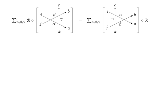
Figure 7.2. A pictorial representation of the quantized Yang-Baxter equation (7.6).

We take the parameters of $\mathscr{L}^{p}_{124}$, $\mathscr{L}^{p}_{135}$, $\mathscr{L}^{p}_{236}$ on both sides of (7.5) to be $(r_{1},s_{1},t_{1},w_{1})$, $(r_{2},s_{2},t_{2},w_{2})$, $(r_{3},s_{3},t_{3},w_{3})$, respectively. From the conservation condition (7.3), the equation (7.6) becomes $0=0$ unless $a+b+c=i+j+k$. There are 20 choices of $(a,b,c,i,j,k)\in\{0,1\}^{6}$ satisfying this condition. Among them, the cases $(0,0,0,0,0,0)$ and $(1,1,1,1,1,1)$ yield the trivial relation $\mathscr{R}(1\otimes 1\otimes 1)=(1\otimes 1\otimes 1)\mathscr{R}$. Thus, there are 18 nontrivial equations for (7.5). They are listed in Appendix D.

Theorem 7.1.

The $RLLL$ relation (7.5) with $p=q$ holds for $\mathscr{R}=R$ in (4.25) under the identification

$$X_{i}={\mathrm{e}}^{u_{i}},\quad Z_{i}={\mathrm{e}}^{-w_{i}},\quad r_{i}={\mathrm{e}}^{c_{i}},\quad s_{i}={\mathrm{e}}^{a_{i}},\quad t_{i}={\mathrm{e}}^{-b_{i}},\quad w_{i}={\mathrm{e}}^{-d_{i}},$$ (7.7)

where $X_{1}=X\otimes 1\otimes 1,X_{2}=1\otimes X\otimes 1,X_{3}=1\otimes 1\otimes X$, and $Z_{i}$ is defined similarly.

Proof.

Write the $RLLL$ relation as $\widehat{R}^{uw}_{456}(\mathscr{L}^{q}_{236}\mathscr{L}^{q}_{135}\mathscr{L}^{q}_{124})=\mathscr{L}^{q}_{124}\mathscr{L}^{q}_{135}\mathscr{L}^{q}_{236}$. The symmetries (4.47)–(4.49) of $\widehat{R}^{uw}$ transform the component equations (D.1)–(D.18) into one another, and it suffices to check one equation in each of the following four groups:

1. (D.1), (D.7), (D.12), (D.18)

2. (D.3), (D.9), (D.10), (D.16)

3. (D.2), (D.4), (D.6), (D.8), (D.11), (D.13), (D.15), (D.17)

4. (D.5), (D.14).

The equations in (1) follow from (4.9) and (4.10). Checking (D.10) is also easy as it is equivalent to $\widehat{R}^{uw}_{123}\circ\phi^{\prime}_{\mathrm{SB}}(Y_{1}^{\prime-1})=\phi_{\mathrm{SB}}\circ\widehat{R}_{123}(Y_{1}^{\prime-1})$. One can verify (D.4) using (D.10) and $\widehat{R}^{uw}_{123}\circ\phi^{\prime}_{\mathrm{SB}}(Y_{6}^{\prime-1})=\phi_{\mathrm{SB}}\circ\widehat{R}_{123}(Y_{6}^{\prime-1})$. Finally, one can show (D.5) by multiplying both sides by $\widehat{R}^{uw}_{123}(Z_{2})$ from the left and expressing the resulting equation with (D.4), (D.11) and(D.16). ∎

The relation (7.7) between parameters agrees with (5.43).

In [16], it has been shown that the solutions $R$ to the $RLLL$ relation for the present $L$ are unique up to normalization within appropriate parity sectors [16]. Thus, Theorem 7.1 effectively identifies the concrete $R$-matrices obtained in [16] with the images of (4.21) in the corresponding representations of the canonical variables. Moreover, Theorem 4.3 verifies the validity of the various tetrahedron equations of the form $RRRR=RRRR$ for these $R$-matrices as conjectured in [16, Sec.6.2].

7.3. $RLLL$ relation for the modular $\mathcal{R}$

Let $\mathcal{V}$ be the space of ket vectors $|x\rangle\,(x\in{\mathbb{C}})$ (cf. Section 6.2) and consider the joint representations of $\mathcal{W}(q)$ and $\mathcal{W}({q^{\vee}})$ on $\mathcal{V}$ given by

$$\pi_{q}: \;\mathcal{W}(q)\rightarrow\mathrm{End}(\mathcal{V}):\quad X|x\rangle={\mathrm{e}}^{\pi{\mathfrak{b}}x}|x\rangle,\qquad Z|x\rangle=|x-i{\mathfrak{b}}\rangle,$$ (7.8)

$$\pi_{q^{\vee}}: \;\mathcal{W}({q^{\vee}})\rightarrow\mathrm{End}(\mathcal{V}):\;\;X|x\rangle={\mathrm{e}}^{\pi{\mathfrak{b}}^{-1}x}|x\rangle,\quad Z|x\rangle=|x-i{\mathfrak{b}}^{-1}\rangle.$$ (7.9)

See (6.1) for the relations between the parameters $q$, $q^{\vee}$ and ${\mathfrak{b}}$. We introduce two $L$-operators that are modular dual to each other as follows:

$$\begin{split}\mathcal{L}^{q}&=(1\otimes 1\otimes\pi_{q})(\mathscr{L}^{q})\in\mathrm{End}(V\otimes V\otimes\mathcal{V}),\\ \mathcal{L}^{q^{\vee}}&=(1\otimes 1\otimes\pi_{q^{\vee}})(\mathscr{L}^{q^{\vee}})\in\mathrm{End}(V\otimes V\otimes\mathcal{V}).\end{split}$$ (7.10)

Since there is no explicit dependence on $p$ in (7.4) or in Figure 7.1, the $RLLL$ relation for the modular $\mathcal{R}$ takes the identical form for either choice $p=q$ or $q^{\vee}$:

Theorem 7.2.

The $R$ matrix $\mathcal{R}$ in Theorem 6.1 satisfies the RLLL relation

$$\mathcal{R}_{456}\mathcal{L}^{p}_{236}\mathcal{L}^{p}_{135}\mathcal{L}^{p}_{124}=\mathcal{L}^{p}_{124}\mathcal{L}^{p}_{135}\mathcal{L}^{p}_{236}\mathcal{R}_{456}$$ (7.11)

for $p=\exp(i\pi{\mathfrak{b}}^{\pm 2})=\begin{pmatrix}q\\ q^{\vee}\end{pmatrix}$ and the parameters $\mathcal{C}_{1}$, $\dotsc$, $\mathcal{C}_{8}$ given by

$$\begin{split}&{\mathrm{e}}^{\pi{\mathfrak{b}}^{\pm 1}{\mathcal{C}}_{1}}=\sqrt{\frac{r_{1}t_{2}w_{3}}{r_{3}t_{1}w_{2}}},\quad\;{\mathrm{e}}^{\pi{\mathfrak{b}}^{\pm 1}{\mathcal{C}}_{2}}=\sqrt{\frac{r_{2}t_{1}w_{3}}{r_{1}r_{3}s_{2}}},\quad{\mathrm{e}}^{\pi{\mathfrak{b}}^{\pm 1}{\mathcal{C}}_{3}}=\sqrt{\frac{r_{1}r_{3}}{r_{2}}},\quad{\mathrm{e}}^{\pi{\mathfrak{b}}^{\pm 1}{\mathcal{C}}_{4}}=\sqrt{\frac{r_{2}s_{2}}{t_{2}w_{2}}},\\ &{\mathrm{e}}^{\pi{\mathfrak{b}}^{\pm 1}{\mathcal{C}}_{5}}=\sqrt{\frac{r_{3}s_{3}w_{1}}{r_{2}w_{3}}},\quad{\mathrm{e}}^{\pi{\mathfrak{b}}^{\pm 1}{\mathcal{C}}_{6}}=\sqrt{\frac{r_{1}s_{1}t_{3}}{r_{2}t_{1}}},\quad\;{\mathrm{e}}^{\pi{\mathfrak{b}}^{\pm 1}{\mathcal{C}}_{7}}=\sqrt{\frac{t_{3}w_{1}}{r_{2}}},\quad{\mathrm{e}}^{\pi{\mathfrak{b}}^{\pm 1}{\mathcal{C}}_{8}}=\sqrt{\frac{r_{1}r_{3}s_{1}s_{3}}{r_{2}t_{1}w_{3}}}.\end{split}$$ (7.12)

Proof.

Note that the parameters (7.12) satisfy the constraint (5.2) Thanks to the modular duality, it suffices to check the $p=q$ case. There are three cases (i), (ii), (iii).

(i) Trivial: (D.1), (D.7), (D.12) and (D.18). They are satisfied due to the presence of the two delta functions in (6.15).

(ii) Easy: (D.4), (D.10), (D.11), (D.13), (D.16), (D.17). They are shown by direct substitution and the recursion relation (6.4). Let us illustrate the calculation along the example of (D.17). The matrix elements of $\mathrm{LHS}-\mathrm{RHS}$ for the transition $|x^{\prime}_{1},x^{\prime}_{2},x^{\prime}_{3}+i{\mathfrak{b}}\rangle\mapsto|x_{1},x_{2},x_{3}\rangle$ is

$$w_{3}{\mathrm{e}}^{\pi{\mathfrak{b}}(x^{\prime}_{3}+i{\mathfrak{b}})}(r_{1}s_{1}+t_{1}w_{1}{\mathrm{e}}^{\pi{\mathfrak{b}}(2x^{\prime}_{1}+i{\mathfrak{b}})})R^{x_{1},x_{2},x_{3}}_{x^{\prime}_{1}+i{\mathfrak{b}},x^{\prime}_{2}-i{\mathfrak{b}},x^{\prime}_{3}+i{\mathfrak{b}}}+s_{2}w_{1}{\mathrm{e}}^{\pi{\mathfrak{b}}x^{\prime}_{1}}R^{x_{1},x_{2},x_{3}}_{x^{\prime}_{1},x^{\prime}_{2},x^{\prime}_{3}}-s_{1}w_{2}{\mathrm{e}}^{\pi{\mathfrak{b}}x_{2}}R^{x_{1},x_{2},x_{3}+i{\mathfrak{b}}}_{x^{\prime}_{1},x^{\prime}_{2},x^{\prime}_{3}+i{\mathfrak{b}}}.$$ (7.13)

Upon substitution of (6.15)–(6.17) and (6.4), this is equal, up to an overall factor, to

$$\int_{-\infty}^{\infty}dz\,{\mathrm{e}}^{2\pi iz(-x_{2}-i\eta+{\mathcal{C}}_{4})}\frac{\Phi_{\mathfrak{b}}(z+\frac{1}{2}(x_{1}-x_{3}+i\eta)+{\mathcal{C}}_{5})\Phi_{\mathfrak{b}}(z+\frac{1}{2}(-x_{1}+x_{3}+i\eta)+{\mathcal{C}}_{6})}{\Phi_{\mathfrak{b}}(z+\frac{1}{2}(x_{1}+x_{3}-i\eta)+{\mathcal{C}}_{7})\Phi_{\mathfrak{b}}(z+\frac{1}{2}(-x^{\prime}_{1}-x^{\prime}_{3}-i\eta)-i{\mathfrak{b}}+{\mathcal{C}}_{8})}\mathcal{D},$$ (7.14)

$$\mathcal{D}={\mathrm{e}}^{\pi{\mathfrak{b}}(-2{\mathcal{C}}_{2}-2{\mathcal{C}}_{3}-x^{\prime}_{1}-2i\eta)}(r_{1}s_{1}+t_{1}w_{1}{\mathrm{e}}^{\pi{\mathfrak{b}}(2x^{\prime}_{1}+i{\mathfrak{b}})})w_{3}+{\mathrm{e}}^{\pi{\mathfrak{b}}x^{\prime}_{1}}(1+{\mathrm{e}}^{\pi{\mathfrak{b}}(2{\mathcal{C}}_{8}-i{\mathfrak{b}}-x^{\prime}_{1}-x^{\prime}_{3}-i\eta+2z)})s_{2}w_{1}$$

$$\qquad-{\mathrm{e}}^{\pi{\mathfrak{b}}({\mathcal{C}}_{1}-{\mathcal{C}}_{2}+{\mathcal{C}}_{4}-x^{\prime}_{1}-2i\eta)}(1+{\mathrm{e}}^{\pi{\mathfrak{b}}(2{\mathcal{C}}_{5}-i{\mathfrak{b}}+x_{1}-x_{3}+i\eta+2z)})s_{1}w_{2}.$$ (7.15)

Under the constraint $x_{1}-x_{3}=x^{\prime}_{1}-x^{\prime}_{3}$ deduced from the two delta functions, $\mathcal{D}=0$ amounts to three equalities ${\mathrm{e}}^{\pi{\mathfrak{b}}({\mathcal{C}}_{2}+2{\mathcal{C}}_{8})}s_{2}w_{1}={\mathrm{e}}^{\pi{\mathfrak{b}}({\mathcal{C}}_{1}+{\mathcal{C}}_{4}+2{\mathcal{C}}_{5})}s_{1}w_{2}$, ${\mathrm{e}}^{\pi{\mathfrak{b}}({\mathcal{C}}_{1}+{\mathcal{C}}_{2}+2{\mathcal{C}}_{3}+{\mathcal{C}}_{4})}w_{2}=r_{1}w_{3}$ and ${\mathrm{e}}^{\pi{\mathfrak{b}}(2{\mathcal{C}}_{2}+2{\mathcal{C}}_{3}+2i\eta)}s_{2}+{\mathrm{e}}^{\pi i{\mathfrak{b}}^{2}}t_{1}w_{3}=0$. They can be confirmed by using (7.12).

(iii) The rest of (D.1)–(D.18). Direct substitution with appropriate shift of the integration variable $z$ and the application of (6.4) similar to case (ii) leads to $\mathrm{LHS}-\mathrm{RHS}=\int_{-\infty}^{\infty}dz\,\Xi(z)$, where $\Xi(z)$ is not identically vanishing. Nevertheless, one can find $\tilde{\Xi}(z)$ such that $\Xi(z)={\tilde{\Xi}}(z)(z+i{\mathfrak{b}})-{\tilde{\Xi}}(z)$. Thus, the claim reduces to the analyticity of ${\tilde{\Xi}}(z)$ in the strip $0<|\mathop{\mathrm{Im}}z|<|\mathrm{Im}(i{\mathfrak{b}})|$ and the damping in $\mathrm{Re}(z)\rightarrow\pm\infty$. As an example, consider (D.6), whose elements of $\text{LHS}-\text{RHS}$ read

$$w_{1}{\mathrm{e}}^{\pi{\mathfrak{b}}(x^{\prime}_{1}-i{\mathfrak{b}})}(r_{2}s_{2}+t_{2}w_{2}{\mathrm{e}}^{\pi{\mathfrak{b}}(2x^{\prime}_{2}+i{\mathfrak{b}})})R^{x_{1},x_{2},x_{3}}_{x^{\prime}_{1}-i{\mathfrak{b}},x^{\prime}_{2}+i{\mathfrak{b}},x^{\prime}_{3}-i{\mathfrak{b}}}\\ +r_{2}w_{3}{\mathrm{e}}^{\pi{\mathfrak{b}}x^{\prime}_{3}}(r_{1}s_{1}+t_{1}w_{1}{\mathrm{e}}^{\pi{\mathfrak{b}}(2x^{\prime}_{1}-i{\mathfrak{b}})})R^{x_{1},x_{2},x_{3}}_{x^{\prime}_{1},x^{\prime}_{2},x^{\prime}_{3}}-r_{3}w_{2}{\mathrm{e}}^{\pi{\mathfrak{b}}x_{2}}(r_{1}s_{1}+t_{1}w_{1}{\mathrm{e}}^{\pi{\mathfrak{b}}(2x_{1}-i{\mathfrak{b}})})R^{x_{1}-i{\mathfrak{b}},x_{2},x_{3}}_{x^{\prime}_{1}-i{\mathfrak{b}},x^{\prime}_{2},x^{\prime}_{3}}.$$ (7.16)

After shifting the integration variable $z$ for the last term to $z+i{\mathfrak{b}}/2$, the integrand for this expression can be shown to be proportional to ${\tilde{\Xi}}(z)(z+i{\mathfrak{b}})-{\tilde{\Xi}}(z)$ with

$${\tilde{\Xi}}(z)={\mathrm{e}}^{2\pi iz(-x_{2}-i\eta+{\mathcal{C}}_{4})}\frac{\Phi_{\mathfrak{b}}(z+\frac{1}{2}(x_{1}-x_{3}+i\eta)+{\mathcal{C}}_{5}-i{\mathfrak{b}})\Phi_{\mathfrak{b}}(z+\frac{1}{2}(-x_{1}+x_{3}+i\eta)+{\mathcal{C}}_{6})}{\Phi_{\mathfrak{b}}(z+\frac{1}{2}(x_{1}+x_{3}-i\eta)+{\mathcal{C}}_{7})\Phi_{\mathfrak{b}}(z+\frac{1}{2}(-x^{\prime}_{1}-x^{\prime}_{3}-i\eta)+{\mathcal{C}}_{8})}.$$ (7.17)

In general, ${\tilde{\Xi}}(z)$ is always found in a similar ‘factorized’ form. ∎

The upper choice of parameters in (7.12) is consistent with (7.7) and (5.43). (Recall the rescaling (6.6).)

Remark 7.3.

As a corollary of Theorem 7.1, it is evident that postulating the $RLLL$ relation (7.11) for $p=q$ and $q^{\vee}$ simultaneously compels ${\mathcal{C}}_{1}=\dotsb={\mathcal{C}}_{8}=0$. The resulting parameter-free (except ${\mathfrak{b}}$) $R$-matrix (6.15)–(6.17) exactly reproduces [2, eq. (51)]. We refer to this particular case as the modular double $\mathcal{R}$.

In Section 6, the term “modular $\mathcal{R}$” (without “double”) is deliberately used to distinctively describe the results with full parameters. Note on the other hand that the condition ${\mathcal{C}}_{1}=\dotsb={\mathcal{C}}_{8}=0$ still leaves five free parameters among $(r_{j},s_{j},t_{j},w_{j})_{j=1,2,3}$.

8. Reduction to the Fock-Goncharov quiver

In this section we explain that our $R$-matrix (4.20) for the symmetric butterfly (SB) quiver reduces to that for the Fock-Gocharov (FG) quiver [10] in a certain limit of parameters.

8.1. $R$-matrix for the FG quiver

Let $\mathrm{p}_{i}$, $\mathrm{u}_{i}$ ($i=1,2,3$) be canonical variables obeying $[\mathrm{p}_{i},\mathrm{u}_{j}]=\delta_{ij}\hbar$, $[\mathrm{p}_{i},\mathrm{p}_{j}]=[\mathrm{u}_{i},\mathrm{u}_{j}]=0$. Recall the $R$-matrix in [10, eq. (4.14)] given as

$$R_{\mathrm{FG}}=\Psi_{q}({\mathrm{e}}^{\theta_{1}-\theta_{3}+\mathrm{p}_{1}+\mathrm{u}_{1}+\mathrm{p}_{3}-\mathrm{u}_{3}-\mathrm{p}_{2}})P_{\mathrm{FG}},\qquad P_{\mathrm{FG}}=\rho_{23}{\mathrm{e}}^{\tfrac{1}{\hbar}\mathrm{p}_{1}(\mathrm{u}_{3}-\mathrm{u}_{2})}{\mathrm{e}}^{\tfrac{\theta_{2}-\theta_{3}}{\hbar}(\mathrm{u}_{3}-\mathrm{u}_{1})},$$ (8.1)

where $\theta_{i}$’ s are parameters. It has been deduced from $\hat{R}_{\mathrm{FG}}=\mathrm{Ad}(R_{\mathrm{FG}})$, where $\hat{R}_{\mathrm{FG}}$ is the cluster transformation corresponding to $\mu^{\ast}_{4}$ in the FG quivers depicted as follows:

(8.2)

As in Figure 3.4, the dots marked $1$, $2$, $3$ in red signify the crossings of the associated wiring diagram, to which the canonical variables are attached.

Let $B_{\mathrm{FG}}$ and $B^{\prime}_{\mathrm{FG}}$ be (the exchange matrices of) the left and the right quivers in (8.2), respectively. Let $\mathcal{Y}(B_{\mathrm{FG}})$ be the skew field generated by $\mathscr{Y}_{1}$, …, $\mathscr{Y}_{5}$ which are attached to the vertices of $B_{\mathrm{FG}}$ and obey the commutation relation (2.1) where $b_{ij}$ is taken to be the elements of $B_{\mathrm{FG}}$. Define $\mathcal{Y}(B^{\prime}_{\mathrm{FG}})$ generated by $\mathscr{Y}^{\prime}_{1}$, …, $\mathscr{Y}^{\prime}_{5}$ from $B^{\prime}_{\mathrm{FG}}$ similarly.

Let $\mathcal{W}^{\mathrm{pu}}_{3}$ be the direct product of the $q$-Weyl algebras generated by ${\mathrm{e}}^{\pm\mathrm{p}_{i}}$, ${\mathrm{e}}^{\pm\mathrm{u}_{i}}$ for $i=1$, $2$, $3$. The fractional field of $\mathcal{W}^{\mathrm{pu}}_{3}$ is denoted by $\mathcal{A}^{\mathrm{pu}}_{3}$. We denote the isomorphism $\pi_{123}$ of $\mathcal{W}^{\mathrm{pu}}_{3}$ [10, eq. (3.7)] (in the sense of exponentials) by $\pi_{\mathrm{FG}}$ and recall the embeddings $\phi_{\mathrm{FG}}\colon\mathcal{Y}(B_{\mathrm{FG}})\hookrightarrow\mathcal{A}^{\mathrm{pu}}_{3}$ and $\phi^{\prime}_{\mathrm{FG}}\colon\mathcal{Y}(B^{\prime}_{\mathrm{FG}})\hookrightarrow\mathcal{A}^{\mathrm{pu}}_{3}$ [10, eq. (3.6)] given as

$$\pi_{\mathrm{FG}}:\begin{cases}\mathrm{p}_{1}\mapsto\mathrm{p}_{1}+\theta_{2}-\theta_{3},\quad\mathrm{p}_{2}\mapsto\mathrm{p}_{1}+\mathrm{p}_{3},\quad\mathrm{p}_{3}\mapsto\mathrm{p}_{2}-\mathrm{p}_{1}-\theta_{2}+\theta_{3},\\ \mathrm{u}_{1}\mapsto\mathrm{u}_{1}+\mathrm{u}_{2}-\mathrm{u}_{3},\quad\mathrm{u}_{2}\mapsto\mathrm{u}_{3},\quad\mathrm{u}_{3}\mapsto\mathrm{u}_{2},\end{cases}$$ (8.3)

$$\phi_{\mathrm{FG}}:\begin{cases}\mathscr{Y}_{1}\mapsto{\mathrm{e}}^{-\theta_{2}+\mathrm{p}_{2}-\mathrm{u}_{2}-\mathrm{p}_{1}},\\ \mathscr{Y}_{2}\mapsto{\mathrm{e}}^{\theta_{2}+\mathrm{p}_{2}+\mathrm{u}_{2}-\mathrm{p}_{3}},\\ \mathscr{Y}_{3}\mapsto{\mathrm{e}}^{-\theta_{1}+\mathrm{p}_{1}-\mathrm{u}_{1}},\\ \mathscr{Y}_{4}\mapsto{\mathrm{e}}^{\theta_{1}-\theta_{3}+\mathrm{p}_{1}+\mathrm{u}_{1}+\mathrm{p}_{3}-\mathrm{u}_{3}-\mathrm{p}_{2}},\\ \mathscr{Y}_{5}\mapsto{\mathrm{e}}^{\theta_{3}+\mathrm{p}_{3}+\mathrm{u}_{3}},\end{cases}\qquad\phi^{\prime}_{\mathrm{FG}}:\begin{cases}\mathscr{Y}^{\prime}_{1}\mapsto{\mathrm{e}}^{-\theta_{3}+\mathrm{p}_{3}-\mathrm{u}_{3}},\\ \mathscr{Y}^{\prime}_{2}\mapsto{\mathrm{e}}^{\theta_{1}+\mathrm{p}_{1}+\mathrm{u}_{1}},\\ \mathscr{Y}^{\prime}_{3}\mapsto{\mathrm{e}}^{-\theta_{2}+\mathrm{p}_{2}-\mathrm{u}_{2}-\mathrm{p}_{3}},\\ \mathscr{Y}^{\prime}_{4}\mapsto{\mathrm{e}}^{-\theta_{1}+\theta_{3}+\mathrm{p}_{3}+\mathrm{u}_{3}+\mathrm{p}_{1}-\mathrm{u}_{1}-\mathrm{p}_{2}},\\ \mathscr{Y}^{\prime}_{5}\mapsto{\mathrm{e}}^{\theta_{2}+\mathrm{p}_{2}+\mathrm{u}_{2}-\mathrm{p}_{1}}.\end{cases}$$ (8.4)

One has $\pi_{\mathrm{FG}}=\mathrm{Ad}(P_{\mathrm{FG}})$. With these notation, the $R$-matrix (8.1) is rephrased as

$$R_{\mathrm{FG}}=\Psi_{q}(\phi_{\mathrm{FG}}(\mathscr{Y}_{4}))P_{\mathrm{FG}}.$$ (8.5)

8.2. Embedding FG into SB

We employ a parallel notation $\mathcal{Y}(B_{\mathrm{SB}})$ and $\mathcal{Y}(B^{\prime}_{\mathrm{SB}})$ to signify the skew fields corresponding to the left and the right quivers in Figure 3.4. It is easy to see that the following maps yield morphisms of the skew fields $\alpha\colon\mathcal{Y}(B_{\mathrm{FG}})\rightarrow\mathcal{Y}(B_{\mathrm{SB}})$ and $\alpha^{\prime}\colon\mathcal{Y}(B^{\prime}_{\mathrm{FG}})\rightarrow\mathcal{Y}(B^{\prime}_{\mathrm{SB}})$:

$$\alpha:\begin{cases}\mathscr{Y}_{1}\mapsto Y_{9},\\ \mathscr{Y}_{2}\mapsto qY_{8}Y_{7},\\ \mathscr{Y}_{3}\mapsto Y_{6},\\ \mathscr{Y}_{4}\mapsto qY_{5}Y_{4},\\ \mathscr{Y}_{5}\mapsto qY_{3}Y_{2},\end{cases}\qquad\alpha^{\prime}:\begin{cases}\mathscr{Y}^{\prime}_{1}\mapsto Y^{\prime}_{9},\\ \mathscr{Y}^{\prime}_{2}\mapsto qY^{\prime}_{5}Y^{\prime}_{7},\\ \mathscr{Y}^{\prime}_{3}\mapsto Y^{\prime}_{6},\\ \mathscr{Y}^{\prime}_{4}\mapsto qY^{\prime}_{3}Y^{\prime}_{4},\\ \mathscr{Y}^{\prime}_{5}\mapsto qY^{\prime}_{8}Y^{\prime}_{2}.\end{cases}$$ (8.6)

Recall that $\mathcal{A}_{3}$ defined after Figure 4.1 for the SB quiver is a fractional field of $\mathcal{W}_{3}$ in which ${\mathrm{e}}^{u_{i}}{\mathrm{e}}^{w_{j}}=q^{\delta_{ij}\hbar}{\mathrm{e}}^{w_{j}}{\mathrm{e}}^{u_{i}}$. On the other hand, $\mathcal{A}^{\mathrm{pu}}_{3}$ for the FG quiver in the previous subsection is a fractional field of $\mathcal{W}^{\mathrm{pu}}_{3}$ in which ${\mathrm{e}}^{\mathrm{p}_{i}}{\mathrm{e}}^{\mathrm{u}_{i}}=q^{\delta_{ij}\hbar}{\mathrm{e}}^{\mathrm{u}_{i}}{\mathrm{e}}^{\mathrm{p}_{i}}$ . Thus there is an isomorphism $\beta\colon\mathcal{W}^{\mathrm{pu}}_{3}\rightarrow\mathcal{W}_{3}$ given by

$$\beta:\mathrm{p}_{i}\mapsto-w_{i},\quad\mathrm{u}_{i}\mapsto u_{i}\quad(i=1,2,3)$$ (8.7)

in the sense of exponentials. We consider the diagram

$$\begin{CD}\mathcal{Y}(B_{\mathrm{FG}})@>{{\alpha}}>{}>\mathcal{Y}(B_{\mathrm{SB}})\\ @V{\phi_{\mathrm{FG}}}V{}V@V{}V{\phi_{\mathrm{SB}}}V\\ \mathcal{W}^{\mathrm{pu}}_{3}@>{\beta}>{}>\mathcal{W}_{3}\\ @V{\pi_{\mathrm{FG}}}V{}V@V{}V{\tau^{uw}_{--++}}V\\ \mathcal{W}^{\mathrm{pu}}_{3}@>{\beta}>{}>\mathcal{W}_{3}\\ @A{\phi^{\prime}_{\mathrm{FG}}}A{}A@A{}A{\phi^{\prime}_{\mathrm{SB}}}A\\ \mathcal{Y}(B^{\prime}_{\mathrm{FG}})@>{{\alpha^{\prime}}}>{}>\mathcal{Y}(B^{\prime}_{\mathrm{SB}})\end{CD}$$ (8.8)

where $\phi_{\mathrm{SB}},\phi^{\prime}_{\mathrm{SB}}$ and $\tau^{uw}_{--++}$ are defined in (4.3), (4.4) and (4.12), respectively.

Proposition 8.1.

The diagram (8.8) is commutative if and only if the parameters $\theta_{i}$ ($i=1$, $2$, $3$) and $(a_{i},b_{i},c_{i},d_{i},e_{i})$ subject to (4.2) satisfy the relations

$$e_{2}=e_{3},\quad a_{1}=-a_{3}=c_{3}=-c_{1},\quad a_{2}=c_{2}=0,$$ (8.9)

$$\theta_{1}=-b_{1},\quad\theta_{2}=-a_{1}-b_{2},\quad\theta_{3}=d_{3}+e_{3}.$$ (8.10)

Proof.

For the top square, it suffices to consider the image of $\mathscr{Y}_{i}\in\mathcal{Y}(B_{\mathrm{FG}})$ ($i=1$, …, $5$). For instance, one has $\phi_{\mathrm{SB}}\circ\alpha(\mathscr{Y}_{1})=\phi_{\mathrm{SB}}(Y_{9})={\mathrm{e}}^{a_{1}+b_{2}+w_{1}-u_{2}-w_{2}}$ and $\beta\circ\phi_{\mathrm{FG}}(\mathscr{Y}_{1})=\beta({\mathrm{e}}^{-\theta_{2}+\mathrm{p}_{2}-\mathrm{u}_{2}-\mathrm{p}_{1}})={\mathrm{e}}^{-\theta_{2}-w_{2}-u_{2}+w_{1}}$, hence the commutativity requires $\theta_{2}=-a_{1}-b_{2}$. A similar calculation leads to

$$\theta_{2}=-a_{1}-b_{2}=e_{2}+d_{2}+a_{3},\quad\theta_{1}=-b_{1},\quad\theta_{1}-\theta_{3}=e_{1}+d_{1}+c_{2}+b_{3},\quad\theta_{3}=e_{3}+d_{3}.$$

For the middle square, it suffices to consider the image of $\mathrm{p}_{i}$, $\mathrm{u}_{i}$, ($i=1$, $2$, $3$). The commutativity leads to

$$\theta_{2}-\theta_{3}=-\lambda_{1}=\lambda_{2},\quad\lambda_{0}=\lambda_{3}=0,$$

where $\lambda_{i}$’s are specified in (4.13). These nine relations are equivalent to (8.9) and (8.10). The commutativity of the bottom square follows from them. ∎

8.3. $R_{\mathrm{FG}}$ as a limit of $R_{\mathrm{SB}}$

Let $R_{\mathrm{SB}}$ be the $R$-matrix (4.20) for the SB quiver under the specialization of the parameters (8.9) and (8.10). Explicitly we have

$$R_{\mathrm{SB}} =\Psi_{q}({\mathrm{e}}^{-\Lambda+e_{1}+u_{1}+u_{3}+w_{1}-w_{2}+w_{3}})^{-1}\Psi_{q}({\mathrm{e}}^{-\Lambda-e_{3}+e_{1}+u_{1}-u_{3}+w_{1}-w_{2}+w_{3}})^{-1}$$

$$\quad\times\Psi_{q}({\mathrm{e}}^{\theta_{1}-\theta_{3}+u_{1}-u_{3}-w_{1}+w_{2}-w_{3}})\Psi_{q}({\mathrm{e}}^{\Lambda+e_{2}+u_{1}+2u_{2}-u_{3}-w_{1}+w_{2}-w_{3}})P_{\mathrm{SB}},$$ (8.11)

$$P_{\mathrm{SB}} ={\mathrm{e}}^{\tfrac{1}{\hbar}(u_{3}-u_{2})w_{1}}{\mathrm{e}}^{\tfrac{\theta_{3}-\theta_{2}}{\hbar}(u_{1}-u_{2})}\rho_{23}=\rho_{23}{\mathrm{e}}^{\tfrac{1}{\hbar}(u_{2}-u_{3})w_{1}}{\mathrm{e}}^{\tfrac{\theta_{3}-\theta_{2}}{\hbar}(u_{1}-u_{3})},$$ (8.12)

where $\Lambda=\theta_{1}-\theta_{3}=d_{1}+e_{1}+c_{2}+b_{3}$. The above formula for $P_{\mathrm{SB}}$ follows from (4.16) under the specialization.

Theorem 8.2.

The $R$-matrix $R_{\mathrm{FG}}$ is reproduced from the specialized $R$-matrix $R_{\mathrm{SB}}$ as

$$\lim R_{\mathrm{SB}}=\beta(R_{\mathrm{FG}}),$$ (8.13)

where the limit is taken as

$$e_{1}\rightarrow-\infty,\;\;e_{2}=e_{3}\rightarrow-\infty,\;\;e_{1}-e_{3}\rightarrow-\infty,\;\;e_{i}+d_{i}=\mathrm{finite}\ (i=1,2,3).$$ (8.14)

Proof.

Since $\Lambda$ remains finite in the limit, one has $\lim R_{\mathrm{SB}}=\Psi_{q}({\mathrm{e}}^{\theta_{1}-\theta_{3}+u_{1}-u_{3}-w_{1}+w_{2}-w_{3}})P_{\mathrm{SB}}$. By comparing this with (8.1), the claim is checked easily. ∎

Remark 8.3.

Parallel results which fit the formula (B.5) can also be formulated. One replaces (8.6) with

$$\alpha:\begin{cases}\mathscr{Y}_{1}\mapsto Y_{7},\\ \mathscr{Y}_{2}\mapsto qY_{8}Y_{9},\\ \mathscr{Y}_{3}\mapsto Y_{2},\\ \mathscr{Y}_{4}\mapsto qY_{3}Y_{4},\\ \mathscr{Y}_{5}\mapsto qY_{5}Y_{6},\end{cases}\qquad\alpha^{\prime}:\begin{cases}\mathscr{Y}^{\prime}_{1}\mapsto Y^{\prime}_{7},\\ \mathscr{Y}^{\prime}_{2}\mapsto qY^{\prime}_{3}Y^{\prime}_{9},\\ \mathscr{Y}^{\prime}_{3}\mapsto Y^{\prime}_{2},\\ \mathscr{Y}^{\prime}_{4}\mapsto qY^{\prime}_{5}Y^{\prime}_{4},\\ \mathscr{Y}^{\prime}_{5}\mapsto qY^{\prime}_{8}Y^{\prime}_{6},\end{cases}$$ (8.15)

and (8.7) with $\beta\colon(\mathrm{p}_{1},\mathrm{p}_{2},\mathrm{p}_{3},\mathrm{u}_{1},\mathrm{u}_{2},\mathrm{u}_{3})\mapsto(-w_{3},-w_{2},-w_{1},u_{3},u_{2},u_{1})$. Then the diagram (8.8) in which $\tau^{uw}_{--++}$ is replaced with $\tau^{uw}_{-+-+}$ (B.1) becomes commutative if and only if (8.9) and $(\theta_{1},\theta_{2},\theta_{3})=(-d_{3},-d_{2}-a_{3},b_{1}+e_{1})$ hold.

8.4. A limiting procedure for modular $R$

Let us demonstrate an explicit limiting procedure that essentially corresponds to Theorem 8.2 in the context of the modular $R$ in the coordinate representation. In the strong coupling regime $0<\eta<1$, one has $|{\mathfrak{b}}|=1$ and $\mathop{\mathrm{Re}}{\mathfrak{b}}>0$. Thus the product representation (6.2) indicates

$$\lim_{z\rightarrow-\infty}\Phi_{\mathfrak{b}}(z)=1.$$ (8.16)

Proposition 8.4.

Specialize the parameters in $\mathcal{C}_{1},\dotsc,\mathcal{C}_{8}$ in Theorem 6.1 as

$$\begin{split}{\mathcal{C}}_{1}&=\frac{1}{2}(\zeta-\xi)\ell_{21}-\frac{1}{2}\zeta\ell_{31},\quad{\mathcal{C}}_{2}=-{\mathcal{C}}_{8}=-T-\frac{1}{2}\zeta\ell_{31},\quad{\mathcal{C}}_{3}=0,\\ {\mathcal{C}}_{4}&=T+\frac{1}{2}(\xi+\zeta)\ell_{21},\quad{\mathcal{C}}_{5}=\frac{1}{2}\zeta\ell_{31},\quad{\mathcal{C}}_{7}={\mathcal{C}}_{5}+{\mathcal{C}}_{6}-{\mathcal{C}}_{8},\end{split}$$ (8.17)

where $\ell_{ij}=\ell_{i}-\ell_{j}$. Then the elements of the $R$-matrix associated with the FG quiver in [10, Prop. 7.4], with the exchange of components $1\leftrightarrow 3$, are reproduced as a limit of (6.15) as follows:

$$\begin{split}\lim_{\begin{subarray}{c}T\rightarrow\infty\\ {\mathcal{C}}_{6},{\mathcal{C}}_{7}\rightarrow-\infty\end{subarray}}{\mathrm{e}}^{-i\pi\gamma}g(\tilde{a},\tilde{b},\tilde{c},\tilde{d})^{-1}{\mathcal{R}}^{x_{1},x_{2},x_{3}}_{x^{\prime}_{1},x^{\prime}_{2},x^{\prime}_{3}}&=\delta(x_{1}+x_{2}-x^{\prime}_{1}-x^{\prime}_{2})\delta(x_{2}+x_{3}-x^{\prime}_{2}-x^{\prime}_{3})\\ &\times\Phi_{\mathfrak{b}}(x_{2}-x^{\prime}_{1}+i\eta-\frac{1}{2}(\xi+\zeta)\ell_{21}){\mathrm{e}}^{i\pi(x_{2}-x^{\prime}_{1}-\xi\ell_{21})(x_{1}-x_{3}+\zeta\ell_{31}-2i\eta)}.\end{split}$$ (8.18)

where $\gamma=-T^{2}+(i\eta-\zeta\ell_{31})T-\tfrac{1}{2}i\eta\ell_{21}(3\xi-\zeta)+\tfrac{1}{2}\ell_{31}\zeta(\ell_{21}(\xi-\zeta)+2i\eta)+\tfrac{1+4\eta^{2}}{12}$.

Proof.

Due to (8.16), in the limit ${\mathcal{C}}_{6},{\mathcal{C}}_{7}\rightarrow-\infty$, the integral $I^{x_{1},x_{2},x_{3}}_{x^{\prime}_{1},x^{\prime}_{2},x^{\prime}_{3}}$ in (6.16) simplifies to

$$I^{x_{1},x_{2},x_{3}}_{x^{\prime}_{1},x^{\prime}_{2},x^{\prime}_{3}} \rightarrow\int_{-\infty}^{\infty}dz{\mathrm{e}}^{2\pi iz(-x_{2}-i\eta+{\mathcal{C}}_{4})}\frac{\Phi_{\mathfrak{b}}(z+\frac{1}{2}(x_{1}-x_{3}+i\eta)+{\mathcal{C}}_{5})}{\Phi_{\mathfrak{b}}(z+\frac{1}{2}(-x^{\prime}_{1}-x^{\prime}_{3}-i\eta)+{\mathcal{C}}_{8})}$$

$$={\mathrm{e}}^{i\pi\nu}\frac{\Phi_{\mathfrak{b}}(x_{2}-x^{\prime}_{1}+i\eta-{\mathcal{C}}_{4}-{\mathcal{C}}_{5}+{\mathcal{C}}_{8})\Phi_{\mathfrak{b}}(x^{\prime}_{1}+{\mathcal{C}}_{5}-{\mathcal{C}}_{8})}{\Phi_{\mathfrak{b}}(x_{2}-{\mathcal{C}}_{4})},$$ (8.19)

where we have evaluated the integral by (C.2), set $x_{1}=x^{\prime}_{1}-x^{\prime}_{3}+x_{3}$ and then applied (6.3) in the result. We omit the messy explicit form of the power $\nu$. Noting that $-{\mathcal{C}}_{4}-{\mathcal{C}}_{5}+{\mathcal{C}}_{8}=-\frac{1}{2}(\xi+\zeta)\ell_{21}$, the rest is straightforward. ∎

In view of the symmetry (4.52) and the comment after Theorem 6.1, one can also reproduce the original form of [10, eq. (7.12)] without the exchange of components $1\leftrightarrow 3$ by specializing the parameters in (6.16) as

$$\begin{split}{\mathcal{C}}_{1}&=\frac{1}{2}(\xi-\zeta)\ell_{23}+\frac{1}{2}\zeta\ell_{13},\quad{\mathcal{C}}_{2}=-{\mathcal{C}}_{8}=-T-\frac{1}{2}\zeta\ell_{13},\quad{\mathcal{C}}_{3}=0,\\ {\mathcal{C}}_{4}&=T+\frac{1}{2}(\xi+\zeta)\ell_{23},\quad{\mathcal{C}}_{6}=\frac{1}{2}\zeta\ell_{13},\quad{\mathcal{C}}_{7}={\mathcal{C}}_{5}+{\mathcal{C}}_{6}-{\mathcal{C}}_{8},\end{split}$$ (8.20)

and taking the limit $-T$, $\mathcal{C}_{5}$, $\mathcal{C}_{7}\rightarrow-\infty$.

These results may be regarded as modular $R$ versions of Theorem 8.2 at the level of matrix elements. In fact, under the specialization (8.9), one has

$$\begin{split}{\mathcal{C}}_{1}&=\frac{1}{2}(\tilde{b}_{1}-\tilde{b}_{2}+2\tilde{c}_{1}+\tilde{d}_{2}-\tilde{d}_{3}),\qquad{\mathcal{C}}_{2}=-\frac{1}{2}(\tilde{b}_{1}+\tilde{d}_{3}),\\ {\mathcal{C}}_{3}&=0,\qquad\qquad\qquad\qquad\qquad\qquad\quad{\mathcal{C}}_{4}=\frac{1}{2}(\tilde{b}_{2}+\tilde{d}_{2}),\\ {\mathcal{C}}_{5}&=\frac{1}{2}(-\tilde{d}_{1}+\tilde{d}_{3}),\quad\qquad\quad\qquad\qquad{\mathcal{C}}_{6}=\frac{1}{2}(\tilde{b}_{1}-\tilde{b}_{3}),\\ {\mathcal{C}}_{7}&=\frac{1}{2}(-\tilde{d}_{1}-\tilde{b}_{3}),\quad\qquad\qquad\qquad\quad\,{\mathcal{C}}_{8}=\frac{1}{2}(\tilde{b}_{1}+\tilde{d}_{3}).\end{split}$$ (8.21)

See (5.1) and (6.6). Then the limit (8.14) with $e_{i}$, $d_{i}$ replaced with $\tilde{e}_{i}$, $\tilde{d}_{i}$ can be identified with $-T$, $\mathcal{C}_{5}$, $\mathcal{C}_{7}\rightarrow-\infty$ for (8.20).

Appendix A Supplement to Section 3.4

The two sides of the inhomogeneous twisted tetrahedron equation (3.24) yield the following monomial transformation:

$$\begin{split}Y^{(22)}_{1}&\mapsto Y_{1},\quad Y^{(22)}_{2}\mapsto Y_{2},\quad Y^{(22)}_{3}\mapsto qY^{-1}_{7}Y^{-1}_{12}Y^{-1}_{13}Y^{-1}_{14},\quad Y^{(22)}_{4}\mapsto Y_{4},\\ Y^{(22)}_{5}&\mapsto q^{-1}Y_{5}Y_{6},\quad Y^{(22)}_{6}\mapsto qY_{13}Y_{14},\quad Y^{(22)}_{7}\mapsto Y^{-1}_{13},\quad Y^{(22)}_{8}\mapsto q^{-1}Y_{12}Y_{13},\quad Y^{(22)}_{9}\mapsto qY_{8}Y_{9},\\ Y^{(22)}_{10}&\mapsto q^{-1}Y_{10}Y_{11},\quad Y^{(22)}_{11}\mapsto Y_{3}Y_{6}Y_{7}Y_{11}Y_{12},\quad Y^{(22)}_{12}\mapsto q^{-3}Y^{-1}_{3}Y^{-1}_{6}Y^{-1}_{7}Y^{-1}_{8}Y^{-1}_{14}Y^{-1}_{15},\\ Y^{(22)}_{13}&\mapsto q^{-1}Y_{3}Y_{6}Y_{7}Y_{8},\quad Y^{(22)}_{14}\mapsto q^{-1}Y^{-1}_{3}Y^{-1}_{6}Y^{-1}_{7}Y^{-1}_{8}Y^{-1}_{11}Y^{-1}_{12},\quad Y^{(22)}_{15}\mapsto q^{-4}Y_{3}Y_{7}Y_{8}Y_{14}Y_{15},\\ Y^{(22)}_{16}&\mapsto qY_{15}Y_{16},\quad Y^{(22)}_{17}\mapsto q^{2}Y_{7}Y_{12}Y_{13}Y_{14}Y_{17}.\end{split}$$ (A.1)

Let us describe the monomial parts $\tau_{-+++}$ and $\tau_{---+}$ in (3.5) mentioned in Proposition 3.8.

$$\tau_{-+++}:\left\{~{}~{}\begin{aligned} Y^{\prime}_{1}&\mapsto Y_{1},\quad&Y^{\prime}_{2}&\mapsto Y_{2}Y_{3}Y_{4},\quad&Y^{\prime}_{3}&\mapsto q^{2}Y_{3}Y_{4}Y_{8},\quad&Y^{\prime}_{4}&\mapsto q^{2}Y^{-1}_{3}Y^{-2}_{4}Y^{-1}_{5}Y^{-1}_{8},\quad&Y^{\prime}_{5}&\mapsto Y_{4}Y_{5}Y_{8},\\ Y^{\prime}_{6}&\mapsto Y_{4}Y_{5}Y_{6},\quad&Y^{\prime}_{7}&\mapsto Y_{7},\quad&Y^{\prime}_{8}&\mapsto Y^{-1}_{4},\quad&Y^{\prime}_{9}&\mapsto Y_{9},\quad&Y^{\prime}_{10}&\mapsto Y_{10},\end{aligned}\right.$$ (A.2)

$$\tau_{---+}:\left\{~{}~{}\begin{aligned} Y^{\prime}_{1}&\mapsto Y_{1},\quad&Y^{\prime}_{2}&\mapsto Y_{2},\quad&Y^{\prime}_{3}&\mapsto q^{-2}Y^{-1}_{4}Y^{-1}_{5}Y_{8},\quad&Y^{\prime}_{4}&\mapsto Y^{-1}_{8},\quad&Y^{\prime}_{5}&\mapsto Y^{-1}_{3}Y^{-1}_{4}Y_{8},\\ Y^{\prime}_{6}&\mapsto Y_{6},\quad&Y^{\prime}_{7}&\mapsto Y_{3}Y_{4}Y_{7},\quad&Y^{\prime}_{8}&\mapsto Y_{3}Y_{4}Y_{5},\quad&Y^{\prime}_{9}&\mapsto q^{-2}Y_{4}Y_{5}Y_{9},\quad&Y^{\prime}_{10}&\mapsto Y_{10},\end{aligned}\right.$$ (A.3)

Note that the image is not necessarily sign coherent.

Appendix B Formulas for $\tau^{uw}_{-+-+}$, $P_{-+-+}$ and $R_{123}$ for $({\varepsilon}_{1},{\varepsilon}_{2},{\varepsilon}_{3},{\varepsilon}_{4})=(-,+,-,+)$

Let $\tau_{-+-+}$ be the one in Example 3.3. Under the parameterization by $q$-Weyl algebra generators (4.3)–(4.4), it is translated into the transformation of the canonical variables as

$$\tau^{uw}_{-+-+}:\;\begin{cases}u_{1}\mapsto u_{2}+\kappa_{0},\qquad\qquad\qquad\;\;w_{1}\mapsto w_{2}-w_{3}+\kappa_{2},\\ u_{2}\mapsto u_{1}-\kappa_{0},\qquad\qquad\qquad\;\;w_{2}\mapsto w_{1}+w_{3}+\kappa_{1},\\ u_{3}\mapsto-u_{1}+u_{2}+u_{3}+\kappa_{0},\quad\;w_{3}\mapsto w_{3}+\kappa_{3},\end{cases}$$ (B.1)

where $\kappa_{r}=\kappa_{r}(\mathscr{P}_{1},\mathscr{P}_{2},\mathscr{P}_{3})$ for $r=0$, $1$, $2$, $3$ is defined, under the condition (4.2), by

$$\kappa_{0}=\frac{e_{2}-e_{1}}{2},\quad\kappa_{1}=c_{1}-c_{2}+c_{3},\quad\kappa_{2}=d_{1}-d_{2}-a_{3}-\kappa_{0},\quad\kappa_{3}=b_{1}+c_{1}-b_{2}-c_{2}-\kappa_{0}.$$ (B.2)

This is realized as an adjoint action as

$$\tau^{uw}_{-+-+} =\mathrm{Ad}(P_{-+-+}),$$ (B.3)

$$P_{-+-+} ={\mathrm{e}}^{\tfrac{1}{\hbar}(u_{1}-u_{2})w_{3}}{\mathrm{e}}^{\tfrac{\kappa_{0}}{\hbar}(w_{1}-w_{2}-w_{3})}{\mathrm{e}}^{\tfrac{1}{\hbar}(\kappa_{1}u_{1}+\kappa_{2}u_{2}+\kappa_{3}u_{3})}\rho_{12}\in N_{3}\rtimes\mathfrak{S}_{3}.$$ (B.4)

From (3.12) and (3.13), the formulas analogous to (4.20) and (4.21) become as follows:

$$\Psi_{q}({\mathrm{e}}^{-d_{1}-c_{2}-b_{3}+u_{1}+u_{3}+w_{1}-w_{2}+w_{3}})^{-1}\Psi_{q}({\mathrm{e}}^{d_{1}+c_{2}+b_{3}+e_{3}-u_{1}+u_{3}-w_{1}+w_{2}-w_{3}})$$

$$\times\Psi_{q}({\mathrm{e}}^{-d_{1}-e_{1}-c_{2}-b_{3}-u_{1}+u_{3}+w_{1}-w_{2}+w_{3}})^{-1}\Psi_{q}({\mathrm{e}}^{d_{1}+c_{2}+e_{2}+b_{3}+e_{3}-u_{1}+2u_{2}+u_{3}-w_{1}+w_{2}-w_{3}})P_{-+-+}$$ (B.5)

$$= \Psi_{q}({\mathrm{e}}^{-d_{1}-c_{2}-b_{3}+u_{1}+u_{3}+w_{1}-w_{2}+w_{3}})^{-1}\Psi_{q}({\mathrm{e}}^{d_{1}+c_{2}+b_{3}+e_{3}-u_{1}+u_{3}-w_{1}+w_{2}-w_{3}})$$

$$\times P_{-+-+}\Psi_{q}({\mathrm{e}}^{b_{1}+a_{2}+d_{3}+e_{3}-u_{1}+u_{3}-w_{1}+w_{2}-w_{3}})^{-1}\Psi_{q}({\mathrm{e}}^{-b_{1}-a_{2}-d_{3}+u_{1}+u_{3}+w_{1}-w_{2}+w_{3}}).$$ (B.6)

Appendix C Integral formula involving non-compact quantum dilogarithm

The following is known as a modular double analogue of the Ramanujan ${}_{1}\Psi_{1}$-sum

$$\int dt\frac{\Phi_{\mathfrak{b}}(t+u)}{\Phi_{\mathfrak{b}}(t+v)}{\mathrm{e}}^{2\pi iwt} =\frac{\Phi_{\mathfrak{b}}(u-v-i\eta)\Phi_{\mathfrak{b}}(w+i\eta)}{K\Phi_{\mathfrak{b}}(u-v+w-i\eta)}{\mathrm{e}}^{-2\pi iw(v+i\eta)}$$ (C.1)

$$=\frac{K\Phi_{\mathfrak{b}}(v-u-w+i\eta)}{\Phi_{\mathfrak{b}}(v-u+i\eta)\Phi_{\mathfrak{b}}(-w-i\eta)}{\mathrm{e}}^{-2\pi iw(u-i\eta)},$$ (C.2)

where $K={\mathrm{e}}^{-i\pi(4\eta^{2}+1)/12}$. See [19, eq. (B.73)] for the condition concerning the validity of the integrals. From $\Phi_{\mathfrak{b}}(u)|_{u\rightarrow-\infty}\rightarrow 1$, their limit $u$, $v\rightarrow-\infty$ reduces to

$$\int dt\frac{{\mathrm{e}}^{2\pi iwt}}{\Phi_{\mathfrak{b}}(t+v)} =\frac{\Phi_{\mathfrak{b}}(w+i\eta)}{K}{\mathrm{e}}^{-2\pi iw(v+i\eta)},$$ (C.3)

$$\int dt\Phi_{\mathfrak{b}}(t+u){\mathrm{e}}^{2\pi iwt} =\frac{K}{\Phi_{\mathfrak{b}}(-w-i\eta)}{\mathrm{e}}^{-2\pi iw(u-i\eta)}.$$ (C.4)

Appendix D Explicit form of $RLLL$ relation (7.5)

We write down the explicit form of (7.5) together with the corresponding choice of $(abcijk)$ in (7.6) or in Figure 7.2. As mentioned after Figure 7.2, there are 18 non-trivial cases. To save the space, we write $Y_{\alpha}=r_{\alpha}s_{\alpha}Z^{-1}+t_{\alpha}w_{\alpha}XZ^{-1}X$.

$$(001001):\, \mathscr{R}(1\otimes X\otimes X)=(1\otimes X\otimes X)\mathscr{R},$$ (D.1)

$$(001010):\, \mathscr{R}\bigl{(}r_{2}t_{1}X\otimes 1\otimes Y_{3}+t_{3}Z\otimes Y_{2}\otimes X\bigr{)}=r_{1}t_{2}\bigl{(}1\otimes X\otimes Y_{3}\bigr{)}\mathscr{R},$$ (D.2)

$$(001100):\, \mathscr{R}\bigl{(}t_{3}w_{1}X\otimes Y_{2}\otimes X+r_{2}Y_{1}\otimes 1\otimes Y_{3}\bigr{)}=r_{1}r_{3}\bigl{(}1\otimes Y_{2}\otimes 1\bigr{)}\mathscr{R},$$ (D.3)

$$(010001):\, r_{1}t_{2}\mathscr{R}(1\otimes X\otimes Z)=\bigl{(}r_{2}t_{1}X\otimes 1\otimes Z+t_{3}Y_{1}\otimes Z\otimes X\bigr{)}\mathscr{R},$$ (D.4)

$$(010010):\, \mathscr{R}\bigl{(}r_{2}t_{1}w_{3}X\otimes 1\otimes X+Z\otimes Y_{2}\otimes Z\bigr{)}=\bigl{(}r_{2}t_{1}w_{3}X\otimes 1\otimes X+Y_{1}\otimes Z\otimes Y_{3}\bigr{)}\mathscr{R},$$ (D.5)

$$(010100):\, \mathscr{R}\bigl{(}w_{1}X\otimes Y_{2}\otimes Z+r_{2}w_{3}Y_{1}\otimes 1\otimes X\bigr{)}=r_{3}w_{2}\bigl{(}Y_{1}\otimes X\otimes 1\bigr{)}\mathscr{R},$$ (D.6)

$$(011011):\, \mathscr{R}(X\otimes X\otimes 1)=(X\otimes X\otimes 1)\mathscr{R},$$ (D.7)

$$(011101):\, s_{3}t_{2}\mathscr{R}\bigl{(}Y_{1}\otimes X\otimes 1\bigr{)}=\bigl{(}t_{1}X\otimes Y_{2}\otimes Z+s_{2}t_{3}Y_{1}\otimes 1\otimes X\bigr{)}\mathscr{R},$$ (D.8)

$$(011110):\, s_{1}s_{3}\mathscr{R}\bigl{(}1\otimes Y_{2}\otimes 1\bigr{)}=\bigl{(}t_{1}w_{3}X\otimes Y_{2}\otimes X+s_{2}Y_{1}\otimes 1\otimes Y_{3}\bigr{)}\mathscr{R},$$ (D.9)

$$(100001):\, r_{1}r_{3}\mathscr{R}(1\otimes Z\otimes 1)=(t_{3}w_{1}X\otimes Z\otimes X+r_{2}Z\otimes 1\otimes Z)\mathscr{R},$$ (D.10)

$$(100010):\, r_{3}w_{2}\mathscr{R}(Z\otimes X\otimes 1)=\bigl{(}w_{1}X\otimes Z\otimes Y_{3}+r_{2}w_{3}Z\otimes 1\otimes X\bigr{)}\mathscr{R},$$ (D.11)

$$(100100):\, \mathscr{R}(X\otimes X\otimes 1)=(X\otimes X\otimes 1)\mathscr{R},$$ (D.12)

$$(101011): \mathscr{R}(t_{1}X\otimes Z\otimes Y_{3}+s_{2}t_{3}Z\otimes 1\otimes X)=s_{3}t_{2}(Z\otimes X\otimes 1)\mathscr{R},$$ (D.13)

$$(101101):\, \mathscr{R}\bigl{(}s_{2}t_{3}w_{1}X\otimes 1\otimes X+Y_{1}\otimes Z\otimes Y_{3}\bigr{)}=\bigl{(}s_{2}t_{3}w_{1}X\otimes 1\otimes X+Z\otimes Y_{2}\otimes Z\bigr{)}\mathscr{R},$$ (D.14)

$$(101110):\, s_{1}w_{2}\mathscr{R}\bigl{(}1\otimes X\otimes Y_{3})=\bigl{(}s_{2}w_{1}X\otimes 1\otimes Y_{3}+w_{3}Z\otimes Y_{2}\otimes X\bigr{)}\mathscr{R},$$ (D.15)

$$(110011):\, \mathscr{R}(t_{1}w_{3}X\otimes Z\otimes X+s_{2}Z\otimes 1\otimes Z)=s_{1}s_{3}(1\otimes Z\otimes 1)\mathscr{R},$$ (D.16)

$$(110101):\, \mathscr{R}\bigl{(}w_{3}Y_{1}\otimes Z\otimes X+s_{2}w_{1}X\otimes 1\otimes Z\bigr{)}=s_{1}w_{2}(1\otimes X\otimes Z)\mathscr{R},$$ (D.17)

$$(110110):\, \mathscr{R}(1\otimes X\otimes X)=(1\otimes X\otimes X)\mathscr{R}.$$ (D.18)

References

- [1] R. J. Baxter, Exactly solved models in statistical mechanics, Academic Press, London (1982)
- [2] V. V. Bazhanov, V. V. Mangazeev, S. M. Sergeev, Quantum geometry of 3-dimensional lattices and tetrahedron equation, 16th Int. Congr. of Mathematical Physics. ed. P. Exner (Singapore: World Scientific) 23–44 (2010)
- [3] V. V. Bazhanov, S. M. Sergeev, Zamolodchikov’s tetrahedron equation and hidden structure of quantum groups, J. Phys. A: Math. Theor. 39 3295–3310 (2006)
- [4] V. V. Fock, A. B. Goncharov, Cluster -varieties, amalgamation and Poisson-Lie groups, Algebraic geometry and number theory, volume 253 of Progr. Math., PP 27–68, Birkhäuser Boston, Boston, MA (2006)
- [5] V. V. Fock, A. B. Goncharov, Cluster ensembles, quantization and the dilogarithm, Ann. Sci. Éc. Norm. Supér. (4) 42 865–930 (2009)
- [6] V. V. Fock, A. B. Goncharov, The quantum dilogarithm and representations of quantum cluster varieties, Invent. Math. 175 no. 2, 223–286 (2009)
- [7] S. Fomin, A. Zelevinsky, Cluster algebras. IV. Coefficients, Compos. Math. 143 no. 1, 112–164 (2007)
- [8] M. Gross, P. Hacking, S. Keel, M. Kontsevich, Canonical bases for cluster algebras, J. Amer. Math. Soc. 31 no. 2, 497–608 (2018).
- [9] A. P. Isaev and P. P. Kulish, Tetrahedron reflection equations, Mod. Phys. Lett. A 12 (1997) 427–437.
- [10] R. Inoue, A. Kuniba, Y. Terashima, Quantum cluster algebras and 3D integrability: Tetrahedron and 3D reflection equations, arXiv:2310.14493.
- [11] R. Inoue, A. Kuniba, Y. Terashima, Tetrahedron equation and quantum cluster algebras, arXiv:2310.14529.
- [12] M. M. Kapranov, V. A. Voevodsky, 2-Categories and Zamolodchikov tetrahedron equations, Proc. Symposia in Pure Math. 56 177–259 (1994)
- [13] R. M. Kashaev, T. Nakanishi, Classical and quantum dilogarithm identities, SIGMA Symmetry Integrability Geom. Methods Appl. 7 Paper 102, 29 pp (2011)
- [14] B. Keller, On cluster theory and quantum dilogarithm identities, in Representations of Algebras and Related Topics, Editors A. Skowroński and K. Yamagata, EMS Series of Congress Reports, European Mathematical Society, 85–11 (2011)
- [15] A. Kuniba, Quantum groups in three-dimensional integrability, Springer, Singapore (2022)
- [16] A. Kuniba, S. Matsuike, A. Yoneyama, New solutions to the tetrahedron equation associated with quantized six-vertex models, Commun. Math. Phys.10.1007/s00220-023-04711-y (2023)
- [17] T. Nakanishi, Synchronicity phenomenon in cluster patterns, J. Lond. Math. Soc. (2) 103 (3), 1120–1152 (2021)
- [18] S. M. Sergeev, Quantum evolution model, J. Phys. A: Math. and Gen. 32 5693 (1999)
- [19] S. M. Sergeev, Arithmetic of quantum integrable systems in multidimensional discrete space-time, unpublished note (2010)
- [20] X. Sun, J. Yagi, Cluster transformations, the tetrahedron equation and three-dimensional gauge theories, arXiv:2211.10702.
- [21] A. B. Zamolodchikov, Tetrahedra equations and integrable systems in three-dimensional space, Soviet Phys. JETP 79 641–664 (1980)