Effective anytime algorithm for multiobjective combinatorial optimization problems

Abstract

In multiobjective optimization, the result of an optimization algorithm is a set of efficient solutions from which the decision maker selects one. It is common that not all the efficient solutions can be computed in a short time and the search algorithm has to be stopped prematurely to analyze the solutions found so far. A set of efficient solutions that are well-spread in the objective space is preferred to provide the decision maker with a great variety of solutions. However, just a few exact algorithms in the literature exist with the ability to provide such a well-spread set of solutions at any moment: we call them anytime algorithms. We propose a new exact anytime algorithm for multiobjective combinatorial optimization combining three novel ideas to enhance the anytime behavior. We compare the proposed algorithm with those in the state-of-the-art for anytime multiobjective combinatorial optimization using a set of 480 instances from different well-known benchmarks and four different performance measures: the overall non-dominated vector generation ratio, the hypervolume, the general spread and the additive epsilon indicator. A comprehensive experimental study reveals that our proposal outperforms the previous algorithms in most of the instances.

1 Introduction

MultiObjective Optimization (MOO) is a field of research with many applications in different areas, such as biology, computer science, scheduling, and finances. Broadly speaking, in a multiobjective optimization problem some objectives are in conflict and they have to be optimized simultaneously. Without loss of generality, we consider minimization problems throughout this paper. In the case of a maximization problem, we use the property $max(f)=-min(-f)$. A MultiObjective Program (MOP) is an optimization problem characterized by multiple and conflicting objective functions that are to be optimized over a feasible set of decisions. If the constraints and the objective functions are linear, the MOP is a MultiObjective Linear Program (MOLP), and when the variables are integer, we name it MultiObjective Integer Program (MOIP). If some variables are constrained to be integer-valued and the rest are continuous, the problem is a MultiObjective Mixed Integer Program (MOMIP). MultiObjective Combinatorial Optimization (MOCO) is a special case of MOIP when the feasible set is finite. MOIP and MOCO are special cases of MultiObjective Discrete Optimization (MODO).

Finding the whole Pareto front in MOCO problems can require too much computational time when a faster solution is needed. For example, one may need to solve an assignment problem in hours and finding the whole Pareto front can take days. In particular, this happens in instances with many non-dominated points, or when the model is hard in itself. From a practical point of view, the decision maker with whom we interact may be interested in a set of solutions as well-spread as possible in the objective space at any time during the search. The concept of anytime algorithms was introduced by Dean and Boddy [dean1988solving] to characterize algorithms with the following two properties: (i) they can be terminated at any time and still return an answer, and (ii) the answers returned improve in some well-behaved manner as a function of time. In a more precise way, algorithms that show a better trade-off between solution quality and runtime are said to have a better anytime behavior [lopez2014automatically].

In this paper we propose a new exact algorithm to solve MOCO problems, which is also valid for MODO problems with finite feasible sets. The fact that the algorithm is exact and all the solutions found are in the Pareto front allows less freedom when interpreting the algorithm and reduces the probability that two different implementations behave differently [rostami2020algorithmic]. The algorithm is anytime in the sense that it is possible to interrupt its execution and take the non-dominated set. Moreover, it is guaranteed that this set is well-spread in the objective space. To check this spread and the quality of the solutions properly, four well-known metrics in the literature have been used: the overall non-dominated vector generation ratio [jiang2014consistencies], the hypervolume indicator [fonseca2006improved, while2012fast], the general spread [jiang2014consistencies, zhou2006combining], and the additive epsilon indicator [liefooghe2016correlation]. In the computational results section, all these metrics are calculated for each of the 480 instances considered in the work presented here.

The proposed algorithm is based on a general framework by Dächert and Klamroth [dachert2015linear]. Broadly speaking, it consists in analyzing a search region in the objective space and looking for new non-dominated points at each iteration. These regions can be considered as boxes in $\mathbb{R}^{p}$, where $p$ is the number of objectives. The contribution of this paper is to present new designing criteria and an innovative way of splitting the objective space so that the solutions obtained are well-spread over the objective space. These are detailed in the following three novel proposals:

• A new strategy to select the appropriate search space region as the next box to explore, in order to guarantee that the new solutions found are spread over the objective space.

• A new way of partitioning the search space after finding a new non-dominated point. This partition reorders the selection of the future boxes to explore and also has an influence in the spread of solutions.

• A new quality function to measure the priority for the new regions to explore.

In order to help readers to reproduce the results of this paper, we uploaded the source code to GitHub. This is a good practice that is becoming popular to face the reproducibility crisis in Computer Science [Hutson725].

The paper is organized as follows. In Section 2, we provide a literature review including the most relevant papers on MOO algorithms that could be used as anytime MOCO algorithms with good spread. In Section 3, we provide the background with some general definitions and the metrics we use in the computational results. In Section 4, a general formulation to solve MOCO problems is given. This formulation is the backbone of our contribution. In Section 5 our new anytime algorithm is presented. An exhaustive computational analysis is shown in Section LABEL:sec:computational_results. The last section is dedicated to the conclusions and future work.

2 Literature review

In this section we review different exact algorithms to solve multiobjective problems. We organize this review in four subsections. The first three subsections cover related works, which are presented (mostly) in chronological order in each subsection. The subsections focus respectively on the first algorithms, the ones based on recursion, and more recent algorithms. The fourth subsection summarizes the algorithms which can be considered as anytime with good spread and that are used to compare with our proposed algorithm.

2.1 First exact algorithms

In 2004, Sylva and Crema [sylva2004method], working on the idea of Klein et al. [klein1982algorithm], designed a new method to solve MultiObjective Integer Linear Programming (MOILP). They partitioned the solution space of dimension $p$ by adding $p$ binary variables and $p$ constraints to exclude the previously-generated non-dominated points. About three years later, Sylva and Crema [sylva2007method] formulated a variant of their previous work, finding well-spread subsets of non-dominated points in MOMIP. If the variables are integer, the whole Pareto front is obtained. To the best of the authors’ knowledge, this was the first work to show dispersed solutions in the objective space, supported by computational results.

Masin and Bukchin [masin2008diversity] developed an algorithm for MOMIP, called DMA (Diversity Maximization Approach), which finds solutions by maximizing a proposed diversity measure and guarantees the generation of the complete set of efficient points.

In 2013, Lokman and Köksalan [lokman2013finding] proposed two improved algorithms based on the work of Sylva and Crema [sylva2004method]. The algorithms iteratively generate non-dominated points and exclude the regions that are dominated by the previously-generated non-dominated points.

Ceyhan et al. [ceyhan2019finding], based on the work of Lokman and Köksalan [lokman2013finding], proposed some algorithms to find a small representative set of non-dominated points for MOMIP. The first of them, called SBA, is able to find the complete Pareto front for discrete problems if enough time is available. The main advantage of the SBA algorithm is that it produces very well-spread solutions over the objective space. As noted in this paper [ceyhan2019finding], the work of Masin and Bukchin [masin2008diversity] is similar to Sylva and Crema’s method in [sylva2007method], because they generate similar representative subsets of non-dominated points for MOMIPs. In fact, SBA outperformed Masin and Bukchin’s algorithm.

2.2 Algorithms based on recursion

In 2003, Tenfelde-Podehl [tenfelde2003recursive] proposed a recursive algorithm for MOCO problems with $p$ criteria. Dhaenens et al. [dhaenens2010k] proposed a new method to solve MOP, called $K$-PPM (Parallel Partitioning Method), which is based on the work of Lemesre et al. [lemesre2007parallel], called 2-PPM and valid only for the bi-objective case. This new approach is valid for any dimension $p\geq 2$, and could also be considered as an extension of the idea of Tenfelde-Podehl [tenfelde2003recursive].

Özlen and Azizoğlu [ozlen2009multi] developed a general approach to generate the Pareto front for MOIP problems, based in the $\varepsilon$-constraint method. They also used recursion to solve multiobjective problems with fewer objectives obtaining efficiency ranges for each objective. One drawback of the method in [ozlen2009multi] is that it generates the same non-dominated point many times. The algorithm was enhanced in the work of Özlen et al. [ozlen2014multi].

2.3 Modern algorithms

Laumanns et al. [laumanns2006efficient, laumanns2005adaptive] proposed the first algorithm to calculate the Pareto front in MOP through the resolution of a number of single-objective problems that depend only on the number of solutions in the front. The work of Laumanns et al. [laumanns2006efficient] was based on the $\varepsilon$-constraint method. They obtained a bound $O(k^{p-1})$ for the number of calls to the single-objective solver, where $k$ is the number of non-dominated points and $p$ the number of objectives. In [laumanns2005adaptive], Laumanns et al. presented another algorithm for solving MOP using only lower bounds (for maximization problems) which leads to a fewer number of constraints. The algorithm by Kirlik and Sayın [kirlik2014new] was an improvement of the work of Laumanns et al. [laumanns2006efficient]. They changed the order in which the subproblems were solved. The search is managed over ($p-1$)-dimensional rectangles.

In the last decade, modern algorithms solving MOO problems have been developed. Apart from the aforementioned work by Ceyhan et al. [ceyhan2019finding], there are other important papers we should mention. Przybylski et al. [przybylski2010recursive] proposed an algorithm to compute the supported non-dominated extreme points for MOIP. This work was generalized by Przybylski et al. [przybylski2010two] to obtain the complete Pareto front for MOIP and is considered as a generalization of the two-phase method of Ulungu and Teghem [ulungu1995two]. Özpeynirci and Köksalan [ozpeynirci2010exact], among other authors, developed an algorithm to generate supported non-dominated points for MOMIP. Dächert and Klamroth [dachert2015linear] conceived an algorithm to solve MOO for $p=3$. Their method is based on the work of Przybylski et al. [przybylski2010recursive] and [przybylski2010two]. They named full m-split the general framework for solving any MOO of dimension $m$. This algorithm, suitably adapted, is used in our work. Later, Klamroth et al. [klamroth2015representation] improved full m-split, developing two new methods, called $RE$ and $RA$, where they were concerned with eliminating or avoiding redundancies in the search zone explorations. Recently, Dächert et al. [dachert2017efficient] have provided new theoretical insights into structural properties of the search region, assuming that a finite set of mutually non-dominated points has already been computed. The work provides better results than those in [klamroth2015representation] for high dimensions ($p\geq 6$). In 2018, Holzmann and Smith [holzmann2018solving] designed an algorithm to solve MODO problems using a weighted augmented Tchebycheff scalarization. This work is also based on the work of Dächert and Klamroth [dachert2015linear]. They improved the results of Kirlik and Sayın [kirlik2014new] and Özlen et al. [ozlen2014multi].

2.4 Related algorithms that can be considered as anytime with good spread

As stated in the preceding review, only a few methods can be considered to have good spread over the objective space. This is in concordance with the work of Ceyhan et al. [ceyhan2019finding], which summarized in two the number of algorithms which can be used to calculate the complete front in MOCO problems [masin2008diversity, sylva2007method]. If fact, with their SBA algorithm, they outperformed the results in [sylva2007method]. The work of Holzmann and Smith [holzmann2018solving] can also be considered as anytime, so we include it in our study.

We analyze which other algorithms in the literature can be slightly modified to obtain a well-spread set of non-dominated points at any time during the search. The algorithms which use the $\varepsilon$-constraint method do not seem to be good at spreading solutions over the objective space, because in the objective function, just one selected objective is optimized (Ch. 4 of [ehrgott2005multicriteria]). Moreover, methods which use branch and bound as the general framework to obtain the Pareto front are widely surpassed by modern algorithms, which avoid repeating solutions [dachert2015linear]. In addition, those which calculate the nadir point in a first phase can be slow because computing the nadir point is an NP-hard problem in itself [gary1979computers], so we do not consider these algorithms.

In conclusion, we have chosen two algorithms: SBA, from the work of Ceyhan et al. [ceyhan2019finding], and the method of Holzmann and Smith [holzmann2018solving]. They are, to the best of the authors’ knowledge, the algorithms that can potentially provide a well-spread set of non-dominated points at any time of execution.

3 Background

In this section, we first present some basic definitions to understand the paper, and then we define the four metrics used for the performance assessment in the computational results.

3.1 Definitions on multiobjective optimization

A MOCO problem can be defined as

$$\min f(x)=(f_{1}(x),\ldots,f_{p}(x)),$$ (1)

$$\textit{ s.t.}\quad x\in X\subset\mathbb{R}^{n},$$ (2)

where $x$ is the decision vector, $p\in\mathbb{N}$ is the number of objectives with $p\geq 2$, $f_{i}:X\rightarrow\mathbb{R}$ with $i=1,\ldots,p$ are the objective functions, and $X\neq\emptyset$ denotes the feasible solution set, which is discrete and bounded.

The notion of optimality with several objective functions is considered in the sense of Pareto optimization. Given two vectors $x,y\in\mathbb{R}^{p}$, we say that $x$ is weakly dominated by $y$ if $y_{i}\leq x_{i}$ for all $i=1,\ldots,p$ (denoted $y\leqq x$). If $y$ weakly dominates $x$ and $y_{k}<x_{k}$ for at least one $k\in\left\{1,\ldots,p\right\}$, then we say that $y$ dominates $x$ (denoted $y\leavevmode\nobreak\ \leq\leavevmode\nobreak\ x$) or $x$ is dominated by $y$. If strict inequality holds for all $k\in\left\{1,\ldots,p\right\}$, then we say that $y$ strictly dominates $x$ (denoted $y<x$) or $x$ is strictly dominated by $y$.

A feasible solution $x\in X$ is an efficient solution if there is no $y\in X$ such that $f(y)$ dominates $f(x)$. A solution $x\in X$ is called weakly efficient if there is no $y\in X$ such that $f(y)$ strictly dominates $f(x)$. The image of an efficient solution $x$ is a non-dominated point, $z=f(x)$. The image of a weakly efficient solution $x\textsc{\char 13\relax}$ is a weakly non-dominated point, $z\textsc{\char 13\relax}=f(x\textsc{\char 13\relax})$ . The set of all efficient solutions in a MOCO problem is called efficient set, $X_{E}$, and its image is the Pareto front, PF$\leavevmode\nobreak\ =\leavevmode\nobreak\ f(X_{E})\subseteq\mathbb{R}^{p}$. An efficient solution is supported if its image lies on the frontier of the convex hull of PF $\subseteq\mathbb{\mathbb{R}}{}^{p}$. Equivalently, $x\in X$ is supported if it minimizes a weighted sum of the $p$ objectives involving positive weights. Due to the fact that, in MOCO, many of the elements in $X_{E}$ could lead to the same image, we are only interested in the set PF and one anti-image for each element of this set.

Let $z^{1},z^{2}\in\mathbb{R}^{p}$. We say that $z^{1}<_{lex}z^{2}$ if there exists an index $q$, where $z^{1}_{q}<z^{2}_{q}$ and $q=min\{k\mid z^{1}_{k}\neq z^{2}_{k}\}$. The symbol $<_{lex}$ represents the strict lexicographic order.

Given a permutation $\sigma$ and a vector function $f:X\rightarrow\mathbb{R}^{p}$, we denote by $f_{\sigma}=(f_{\sigma(1)},f_{\sigma(2)},\ldots,f_{\sigma(p)})$ the vector function where the objectives are reordered using $\sigma$. We say that $x\in X$ is a lexicographic optimal solution for permutation $\sigma$ if there is no $y\in X$ with $f_{\sigma}(y)<_{lex}f_{\sigma}(x)$. There exists a maximum of $p!$ different lexicographic optimal solutions, one for each permutation.

Given a Pareto front, PF, the ideal point is $z^{I}=(z^{I}_{1},z^{I}_{2},\ldots,z^{I}_{p})$, where $z^{I}_{i}=$ $\displaystyle\min_{x\in X}f_{i}(x)=$ $\displaystyle\min_{z\in PF}z_{i},$    $\forall i=1,\ldots,p$, and the nadir point is $z^{N}=(z^{N}_{1},z^{N}_{2},\ldots,z^{N}_{p})$, where $z^{N}_{i}=\displaystyle\max_{x\in X_{E}}f_{i}(x)=\max_{z\in PF}z_{i},\,\,\forall i=1,\ldots,p$. It is clear that $z^{I}$ and $z^{N}$ are a lower and an upper bound for the Pareto front. While the ideal point is found by solving $p$ single objective optimization problems, the computation of the nadir point without knowing the whole Pareto front involves optimization over the efficient set, a very difficult problem in general [ehrgott2003computation].

Although it is common to use the term ‘efficient solution’ in the decision space and ‘non-dominated point’ in the objective space, sometimes we use the term ‘solution’ to refer to both spaces, when there is no possible confusion. We assume that $|PF|$ $>1$, otherwise the problem can be solved in one iteration with a single-objective optimization technique.

Given two vectors $l,u\in\mathbb{R}^{p}$ with $l<u$, we define the box $[l,u]$ as:

$$[l,u]=\{x\in\mathbb{R}^{p}\mid l_{i}\leq x<u_{i},\,\forall i=1,\ldots,p\}.$$ (3)

When the lower bound of a box is the ideal point in a Pareto front, we usually represent the box only with its upper bound, that is, $[z^{I},u]=[u]$.

3.2 Performance assessment

The performance assessment of algorithms for multiobjective optimization is not a trivial issue. A good analysis comparing different multiobjective evolutionary algorithms is given in [zitzler2003performance]. Recently, Li and Yao [li2019quality] published a survey of the quality evaluation for 100 different metrics. In [jiang2014consistencies], Jiang et al. categorize the MOO metrics into four groups: capacity metrics, convergence metrics, diversity metrics, and convergence-diversity metrics. Despite the aforementioned difficulty of designing anytime algorithms with good spread (effective anytime algorithms) because performance is often evaluated subjectively (see [lopez2014automatically]), we have tried to take a representative group of metrics in which we can assume that the better the value of these metrics, the better the performance of the algorithm. Thus, we take one metric from each of the four categories defined by Jiang et al.

Capacity metrics [jiang2014consistencies] quantify the number or ratio of non-dominated solutions. We use here the Overall Non-dominated Vector Generation Ratio, which is defined as

$$\text{ONVGR}(N)=\frac{|N|}{|PF|},$$ (4)

where $N\subseteq PF$ is the set of non-dominated solutions found by a run of a search algorithm and $|\cdot|$ is the cardinality of a set. Thus, ONVGR is a rational number in the interval $[0,1]$ that represents the fraction of points of the Pareto front that were found by the search algorithm. For computing ONVGR, we need to know the total number of points in the Pareto front.

Convergence metrics measure the degree of proximity of the set of solutions to the complete front. The additive epsilon indicator gives the minimum additive factor by which the approximation set has to be translated in the objective space in order to weakly dominate the reference set [zitzler2003performance, liefooghe2016correlation]. We have scaled each objective to obtain a value in the range [0,1]. This additive epsilon indicator is defined as

$$\varepsilon_{+}(N)=\max_{x\in PF}\min_{y\in N}\max_{i=1,\ldots,p}\left(\frac{y_{i}-x_{i}}{r_{i}}\right),$$ (5)

where $r_{i}$ is the range of objective $i$ in N. This metric is also used in the computational experiments conducted by Ceyhan et al. [ceyhan2019finding] with the name of coverage gap.

Diversity metrics indicate the distribution and spread of solutions. From this group, we have selected the general spread metric, also cited in [jiang2014consistencies]. The original spread metric (Deb et al. [deb2000fast]) calculates the distance between two consecutive solutions, which only works for 2-objective problems. An extension to any dimension, defined in [zhou2006combining], computes the distance from a point to its nearest neighbor. Let $N$ be a set of non-dominated points and $\{e_{i}\}_{i=1}^{m}$ the extreme solutions, which are the images of the lexicographic optimal solutions of the complete Pareto front, $\bS{d}=\frac{1}{\lvert N\lvert}\sum_{x\in N}d(x,N)$, where $\displaystyle d(x,N)=\min_{y\in N;y\neq x}d^{*}(x,y)$ and $d^{*}$ denotes the Euclidean distance between two $p$-dimensional vectors. We define the general spread as

$$\Delta^{*}(N)=\frac{\sum_{i=1}^{m}d(e_{i},N)+\sum_{x\in N}\lvert d(x,N)-\bS{d}\lvert}{\sum_{i=1}^{m}d(e_{i},N)+\lvert N\lvert\bS{d}}.$$ (6)

Note that the metric $\Delta^{*}$ is a non-negative number. The lower its value, the more well-spread is $N$. Every lexicographic optimal solution not obtained in the execution produces a positive value in $\sum_{i=1}^{m}d(e_{i},N)$ and a higher value for $\Delta^{*}$.

From the group of convergence-diversity metrics we have selected the hypervolume indicator. Given a set of $d$ non-dominated points, N$=\{z^{1},z^{2},\ldots,z^{d}\}$, the hypervolume HV is the measure of the region which is simultaneously dominated by N and bounded by a reference point $r\in\mathbb{R}^{p}$:

$$\text{HV}(N,r)=volume\left(\bigcup_{j=1}^{d}[z^{j},r]\right),$$ (7)

where $volume$ is the Lebesgue measure in $\mathbb{R}^{p}$. This is the quality measure with the highest discriminatory power among the known unary quality measures [lopez2014automatically, rostami2017fast, zitzler2003performance]. There are many software packages that calculate the exact hypervolume, given a non-dominated set and a reference point [fonseca2006improved, while2012fast]. The reference point can be taken as $r_{i}=\displaystyle\max_{j=1,\ldots,d}z^{j}_{i}$ $\quad\forall i=1,\ldots,p$. This is an acceptable choice when we have no information about the complete Pareto front. In the computational experiments presented in this paper, we have calculated the complete fronts for all the instances in order to have a fitted reference point. This means that we know the nadir point for every instance. As noted in the work of Li and Yao [li2019quality], there is still no consensus on how to choose a proper reference point for a given problem. To assign some importance to the extreme points, we add one unit to the nadir point, so the reference point is $r_{i}=z^{N}_{i}+1\quad\forall i=1,\ldots,p$. Sometimes, it is useful to consider the percentage of the total hypervolume reached:

$$\text{HVR}(N,r)=\frac{\text{HV}(N,r)}{\text{HV}(\text{\emph{PF}},r)}.$$ (8)

Given two subsets of non-dominated points, $A$ and $B$, we write $A\succeq B$ if every $z^{2}\in B$ is weakly dominated by at least one $z^{1}\in A$. A metric is Pareto compliant if, for every two subsets $A$ and $B$ with $A\succeq B$ and $B\nsucceq A$, the metric value for $A$ is not worse than the metric value for $B$. It is desirable for a metric to be Pareto compliant [zitzler2007hypervolume]. In other words, it must not contradict the order induced by the Pareto dominance relation. Of the four metrics considered, ONVGR, HV and $\varepsilon_{+}$ are Pareto compliant. This is equivalent to saying that, if we add a new element to the subset of solutions, then ONVGR and HV do not decrease and $\varepsilon_{+}$ does not increase. Nevertheless, $\Delta^{*}$ is not Pareto compliant, and we have to be more careful with its analysis.

4 General formulation for solving MOCO problems

In this section we describe the framework of Dächert and Klamroth [dachert2015linear] to solve MOCO problems. The framework can be found in Algorithm 1. Our proposed algorithm, described in Section 5, is based on this framework, but we add three modifications that let us get a better spread of solutions over the objective space. The method used by Holzmann and Smith [holzmann2018solving] is also based on this framework. The idea of the method is to maintain a set of search zones, $\mathfrak{U}$, which are $p$-dimensional boxes. Every search zone is defined by its upper bound, because we can consider that the ideal point is the lower bound.

Algorithm 1 General method for MOCO problems

0:  $P$

0:  $N$

1:  $N=\emptyset$

2:  $\mathfrak{U}\leftarrow\{U\}$

3:  while ($\mathfrak{U}\neq\emptyset$) do

4:     Select $B\in\mathfrak{U}$

5:     if  (P($B$) is feasible) then

6:        $x^{*}\leftarrow$ Optimal solution of $P(B)$

7:        N = N $\cup$ $\left\{f(x^{*})\right\}$

8:        Update $\mathfrak{U}$

9:     else

10:        $\mathfrak{U}\leftarrow\mathfrak{U}-\{B\}$

11:     end if

12:  end while

At the beginning, the set $N$, containing the non-dominated points, is empty (Line  1), and the set of search zones contains the initial element $U$ (Line 2), defined by an upper bound of the nadir point. The mathematical program used by the algorithm, $P$, is an input parameter. The algorithm then enters a loop while there is at least one zone to analyze. In each iteration of the loop it selects one zone (Line 4), solves the optimization problem, and, if a new non-dominated point is found, it is saved in $N$. Every time it finds a new non-dominated point, it updates the set $\mathfrak{U}$ accordingly (Line 8), so as to prevent repeated solutions in the future. Another goal of the updating procedure is to reduce the number of search regions at each iteration. More specifically, at least box $B$ is extracted from $\mathfrak{U}$. The algorithm ends because, in MOCO problems, the number of non-dominated points is finite.

In what follows, we study the relevant elements of Algorithm 1 and analyze different options which may produce a well-spread set of solutions if we treat it as an anytime algorithm. We focus on three aspects of the general method that we think are important to consider.

4.1 Mathematical program

The selected mathematical program is one of the key aspects of the algorithm. Not all methods that solve multiobjective problems have the same performance. In fact, those which are based on the $\varepsilon$-constraint method (Ch. 4 of [ehrgott2005multicriteria]) should not be good as effective anytime algorithms, unless we use a strategy for the selection of the next search zone to explore that guarantees a good dispersion of solutions in the objective space. The mathematical program used in the SBA method by Ceyhan et al. [ceyhan2019finding] is:

$$\min_{x\in X}\left(\varepsilon\sum_{i=1}^{p}w_{i}f_{i}(x)-\alpha\right),$$ (9)

$$\textit{ s.t.}\quad\,f_{i}(x)\leq u_{i}-\alpha,\quad i=1,\ldots,p,$$ (10)

$$\qquad\quad\alpha\geq 0,$$ (11)

where $\alpha$ is a variable which represents the coverage gap, $\varepsilon$ is a sufficiently small positive constant and $\omega_{i}>0\,\,\forall i$. If the program (9) to (11) has a solution, then it is efficient.

Another mathematical program, used in the work of Holzmann and Smith [holzmann2018solving], is based on a weighted augmented Tchebycheff norm:

$$\min_{x\in X}\left(\max_{i=1,\ldots,p}\left(\omega_{i}\left\lvert f_{i}(x)-z_{i}^{I}\right\lvert\right)+\epsilon\cdot\sum_{i=1}^{p}\omega_{i}\left\lvert f_{i}(x)-z_{i}^{I}\right\lvert\right),$$ (12)

where $z^{I}$ is the ideal point of the problem. The parameters $\omega$ and $\epsilon$ are chosen to make the program feasible. Depending on the objective value, we conclude whether the problem has a new solution inside the box or not. The reader is referred to the original paper [holzmann2018solving] for more information.

We observed relevant performance differences between the two programs in a preliminary study. The weighted augmented Tchebycheff norm behaves better regarding the spread of the solutions in the objective space.

4.2 Selection of the next search zone to explore

Line 4 of Algorithm 1 proposes the extraction of the next search zone to analyze. The selection may be done randomly, but intuitively, if we split the objective space into different regions, and at each step we explore those which have a higher volume, we expect to obtain a final better spread of the solutions. Following this idea, we can define a numerical value for each search zone, called priority. One example of the priority function is the volume of the $p$-dimensional hyperrectangle with opposite vertices being the vector $u$ (upper bound for the search zone) and $z^{I}$ (ideal point). For instance, if $u=(10,20,30)$ and $z^{I}=(5,12,20)$, then the volume of the box is $(10-5)\cdot(20-12)\cdot(30-20)=400$, and this could be its priority. A more sophisticated way of selecting the next box to explore is mentioned in Section 5.1.

4.3 Updating the set of search zones

This may be the most important aspect to take into account in Algorithm 1 (Line 8) in terms of termination of the general algorithm and computational effort. One way to ensure that a non-dominated point is never computed again during the search consists in splitting the objective search zone and discarding at least that point. A good way to do this is found in the work of Dächert and Klamroth [dachert2015linear]. After a solution $z$ is found, they divide the search zone into $p$ new zones. The union of the new search zones discards the points dominated by $z$ and the new search regions to explore contain at least one point less than the original search region. Given a box $B$ with upper bound $u=(u_{1},\ldots,u_{p})$, let us suppose that we solve the mathematical problem and obtain a new non-dominated point $z=(z_{1},\ldots,z_{p})$. Then, we split the box $B$ into $\left\{B_{i}\right\}_{i=1}^{p}$ with upper bounds $\left\{u^{i}\right\}_{i=1}^{p}$, being $u^{i}=\left(u_{1},\ldots,u_{i-1},z_{i},u_{i+1},\ldots,u_{p}\right)\forall i=1,\ldots,p$. Each box $B_{i}$ with upper bound $u^{i}$ is said to have direction $i$. If the lower bound of all the boxes $B$ and $B_{i}$ is the ideal point, $z^{I}$, we call the split full p-split. A graphical example is shown in Figures 1 and 1 for $p=3$. Note that when a new non-dominated point is obtained, we must apply full p-split to all search zones that contain that new point, in order to assure the non-duplicity of the solutions. Full p-split is used in the work of Holzmann and Smith [holzmann2018solving]. In Section 5.2 we describe a new way of splitting the objective space, called p-partition.

The splitting process often generates redundant zones. If we have two search zones $u^{1},\,u^{2}$ with $u^{1}\leq u^{2}$, all potential non-dominated points generated by $u^{1}$ could also be generated by $u^{2}$, which means that $u^{1}$ is redundant. Therefore, a filtering process should be implemented after the split. Klamroth et al. [klamroth2015representation] proposed two different algorithms for this purpose. The first is called RE (redundancy elimination) and consists in eliminating those redundant search zones at each iteration. The second algorithm is called RA (redundancy avoidance) and is based on structural properties of local upper bounds which yield necessary and sufficient conditions for a candidate local upper bound to be non-redundant. The filtering step is avoided in this case. In the computational experiments of the work by Klamroth et al. [klamroth2015representation], they obtained better results in runtimes using RE when $p\in\{3,4,5\}$, and using RA when $p>5$.

A more recent paper by Dächert et al. [dachert2017efficient] describes a specific neighborhood structure among local upper bounds. With this structure, updates to the search region when a new non-dominated point is found can be more efficient compared to RE and RA approaches, as the number of points increases, but RA and even RE perform better for a small number of solutions. Since our proposal is designed as an anytime algorithm where the decision maker can stop the execution whenever desired, it is reasonable to think that the total number of solutions may not be high, unless a complete execution is derived. Thus, we have decided to use the RE approach in this paper.

5 Proposed anytime algorithm: TPA

In this section, we propose a new exact anytime algorithm based on the general framework described in Section 4 but with three novel contributions. This algorithm can solve any MOCO problem and it can also be used for MODO problems with finite feasible sets. We call it TPA because it uses a Tchebycheff mathematical program with Partition of the objective space using Alternating of directions. The pseudocode is shown in Algorithm 2.

Algorithm 2 TPA

0:  $f$ and $X$  // The MOCO problem

0:  $XZ$   // A set of efficient solutions and their image

1:  $\mathfrak{L}=\left(\mathfrak{L}_{1},\ldots,\mathfrak{L}_{p}\right)$  and  $\mathfrak{L}_{i}=\emptyset,\quad\forall i=1,\ldots,p$

2:  $XZ=\emptyset$

3:  $k=0$

4:  Compute the ideal point and an estimation of the nadir point: $z^{I}$ and $\overline{z}^{N}$

5:  Set $\epsilon=1/(2p(r-1))$ where $r=\max_{i=1}^{p}\left\{\overline{z}^{N}-z^{I}\right\}$

6:  $\mathfrak{L}_{1}.insert\left(\left[z^{I},\overline{z}^{N}\right]\right)$

7:  $P(u,\omega)\equiv\displaystyle\min_{x\in X}\left(\max_{i=1,\ldots,p}\left(\omega_{i}\left\lvert f_{i}(x)-z_{i}^{I}\right\lvert\right)+\epsilon\cdot\sum_{i=1}^{p}\omega_{i}\left\lvert f_{i}(x)-z_{i}^{I}\right\lvert\right)$

8:  while $\exists\,i:|\mathfrak{L}_{i}|>0$ and $intime$ do

9:     $(B,k)\leftarrow$ Select_next_box($\mathfrak{L}$, $k$)

10:     Set $\omega=(\omega_{1},\ldots,\omega_{p})$ where $\omega_{i}=1/\max\{1,B.u_{i}-z^{I}_{i}\}$

11:     $(x^{*},obj)$ $\leftarrow$ Solve $P(B.u,\omega)$

12:     if  $obj<1$ and $z^{I}<B.u$ then

13:        XZ $\leftarrow$ XZ $\cup$ $\left\{\left(x^{*},f(x^{*})\right)\right\}$

14:        Update $\left(\mathfrak{L},f(x^{*})\right)$

15:     else

16:        $\mathfrak{L}_{k}.remove(B)$

17:     end if

18:  end while

We now provide a high-level description of the algorithm and go in depth into the novel contributions in separate subsections. Every search zone is a box with the following fields: lower bound ($l$), upper bound ($u$), and priority. The vector $\mathfrak{L}$ contains $p$ priority queues (heaps) of boxes. The boxes in queue $\mathfrak{L}_{i}$ have direction $i$ and are sorted by non-increasing priority. The initial box has as lower and upper bounds the ideal point and an upper bound of the nadir point. Thus, it contains the whole Pareto front. We insert this box into $\mathfrak{L}_{1}$ (Line 6), although any other queue $\mathfrak{L_{i}}$ could be chosen. The $\epsilon$ value is constant during the execution and depends on the initial bounds (Line 5).

TPA then executes a loop while there is a box in any list of $\mathfrak{L}$ and the time limit is not reached (Boolean intime). In the loop, it first selects the next box to analyze (Line 9) using Algorithm 3. Then, it solves the mathematical program in Eq. (12) (Line 7). As pointed in Section 4, this mathematical program provides better spread of the non-dominated points. The parameters are taken from the work of Holzmann and Smith [holzmann2018solving]: $\omega_{i}=1/\max\{1,u_{i}-z_{i}^{I}\},\,\forall i$, and $\epsilon=1/(2p(r-1))$, where $u$ is the upper bound of the next box to analyze, $r=\max_{i=1,\ldots,p}(\overline{z}^{N}_{i}-z^{I}_{i})$, $z^{I}$ is the ideal point and $\overline{z}^{N}$ is an upper bound of the nadir point, computed as follows:

$$\overline{z}^{N}_{i}=\max_{x\in X}(f_{i}(x))\qquad\forall i=1,\ldots,p.$$ (13)

When $u\in\left[\overline{z}^{N}\right]$, the model is always feasible. Moreover, if $z^{I}<u$ the solution is inside the box $[u]$ if and only if the objective value is less than one unit (Theorem 5 of [holzmann2018solving]). Thus, we can slightly modify Line 5 of Algorithm 1, changing the expression ‘is feasible’ by ‘$obj<1$ and $z^{I}<u$’ (Line 12 of Algorithm 2). If it finds a new solution, $x^{*}$, it adds the pair $(x^{*},f(x^{*}))$ to $XZ$ (Line 13) and updates the boxes in the priority queues $\mathfrak{L}$ (Line 14). Otherwise, it discards the box from the corresponding queue (Line 16).

The correctness and termination of TPA is proven in Theorem 1. This is an exact anytime algorithm and, thus, the complete Pareto front is found if the algorithm is given enough time. This guarantees the optimality and convergence of the algorithm. Observe that all the solutions found belong to the Pareto front. This contrasts with other heuristic and metaheuristic algorithms that can only compute approximate solutions without any guarantee of being efficient. Such algorithms require mechanisms to explore the search space that can be interpreted differently by different developers. Rostami et al. [rostami2020algorithmic] have recently studied this issue and found that the resulting approximate solutions can influence the final results in such a way that the differences in quality metrics can even be statistically significant. The reliability and stability of TPA are supported by the ILP solver used. The memory usage and computation time are proportional to the number of boxes to maintain, and this can be exponential in the number of solutions found. Furthermore, the number of solutions in the Pareto front can be exponential in the number of decision variables. Thus, the memory required by the algorithm and the run time can be exponential in the number of variables if the whole Pareto front is computed. Regarding memory usage, in our experiments, using 2 GB of RAM was enough even when the complete Pareto front was computed.

In the next subsections we will detail the three novel contributions of the algorithm: a method to diversify the search exploring boxes with different directions, a new way to split the boxes forming a partition of the original one, and a new priority function for the boxes to explore.

5.1 Alternation of directions in the search

In this section we propose a new strategy for the selection of the next box to explore, trying to diversify the regions of the objective space that are explored. This is the first novel contribution of this paper. The priority queue $\mathfrak{L}_{i}$ contains boxes with direction $i$. Boxes in different directions are displaced in the objective space along the different dimensions. We propose to select a box from a different priory queue $\mathfrak{L}_{i}$ in each iteration of TPA. Among the ones with the same direction TPA chooses the box with higher priority. The pseudo-code of the Select_next_box procedure (Line 9 in Algorithm 2) is in Algorithm 3.

Algorithm 3 Select_next_box

0:  $\left\{\mathfrak{L}_{i}\right\}$, $k$   // List of boxes and integer counter

0:  $(B,k)$

1:  $B=\emptyset$

2:  if $\exists\,i:|\mathfrak{L}_{i}|>0$ then

3:     $k=(k\mod p)+1$

4:     while $|\mathfrak{L}_{k}|=0$ do

5:        $k=(k\mod p)+1$

6:     end while

7:     $B\leftarrow\text{argmax}_{B\in\mathfrak{L}_{k}}\left(B.priority\right)$

8:  end if

5.2 New updating procedure of the search zone

This section presents a new way of splitting the box, called p-partition. This is the second contribution of the paper. The main difference between p-partition and full p-split is that the new boxes created by p-partition form a partition of the original box (they are pairwise disjoint).

Definition 1.

Let $B=[l,u]$ be a box and $z\in\mathbb{R}^{p}$ a point. For every $i=1,\ldots,p$, we define $B_{i}(z)=\left\{x\in B\mid x_{i}<z_{i}\text{ and }x_{j}\geq z_{j}\,\forall j>i\right\}$. We also define $B_{0}(z)$=$\{x\in B$ $\mid x_{j}$ $\geq z_{j}$ $\,\forall j\}$.

It is easy to check that $B_{i}(z)$ are boxes, which can be written as follows:

$$B_{i}(z)=\left[\left(l_{1},\ldots,l_{i},\hat{z}_{i+1},\ldots,\hat{z}_{p}\right),\left(u_{1},\ldots,u_{i-1},\hat{z}_{i},u_{i+1},\ldots,u_{p}\right)\right],$$ (14)

where $\hat{z}_{i}=\max\{z_{i},l_{i}\}$ $\forall i=1,\ldots,p$. If $B_{i}(z)\neq\emptyset$, then it has direction $i$.

Proposition 1.

Given a box $B$, then $\left\{B_{i}(z)\right\}_{i=0}^{p}$ is a partition of $B$.

Proof.

We need to prove that $B_{i}(z)\cap B_{j}(z)=\emptyset\,\,\text{for all }i\neq j$ and $\bigcup\limits^{p}_{i=0}B_{i}(z)=B$. Suppose $x\in B_{i}(z)\cap B_{j}(z)$ for indexes $i,j$ with $i<j$. As $x\in B_{i}(z)$, then $x_{j}\geq z_{j}$. As $x\in B_{j}(z)$, then $x_{j}<z_{j}$. This is a contradiction, so the sets are always disjoint and the first part is proved.

Let $x\in\bigcup\limits^{p}_{i=0}B_{i}(z)$. By definition, $x\in B$, so $\bigcup\limits^{p}_{i=0}B_{i}(z)\subset B$. Now let $x\in B$. If $x_{i}\geq z_{i}\,\,\forall i$, then $x\in B_{0}(z)$. Otherwise, let $j$ be the higher index which verifies $x_{j}<z_{j}$. Then, $x\in B_{j}(z)\subset\bigcup\limits^{p}_{i=0}B_{i}(z)$, so $\bigcup\limits^{p}_{i=0}B_{i}(z)=B$ and the second part is proved. ∎

Definition 2.

Let $B=[l,u]$ be a box, and $z<B.u$. We define the p-partition of the box $B$ according to $z$ as $\left\{B_{i}(z)\right\}_{i=1}^{p}$.

When obtaining a non-dominated point $z$, the exploration of some other boxes in the future might produce the same solution. In order to prevent this, we split those boxes and remove the space weakly dominated by $z$, which is $B_{0}(z)$. That is why p-partition does not include $B_{0}(z)$.

Figure 1 shows a graphical example of p-partition compared to full p-split. Note that the upper bounds in the resulting boxes are the same, but lower bounds are different.

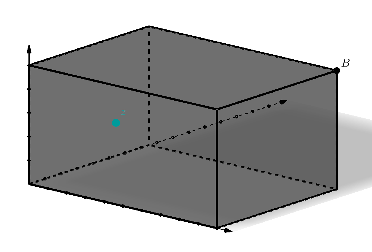
(a) Box $\mathbf{B}=[(0,0,0),\,(20,15,10)]$ with non-dominated point $z=\leavevmode\nobreak\ (5,5,5)$ inside.

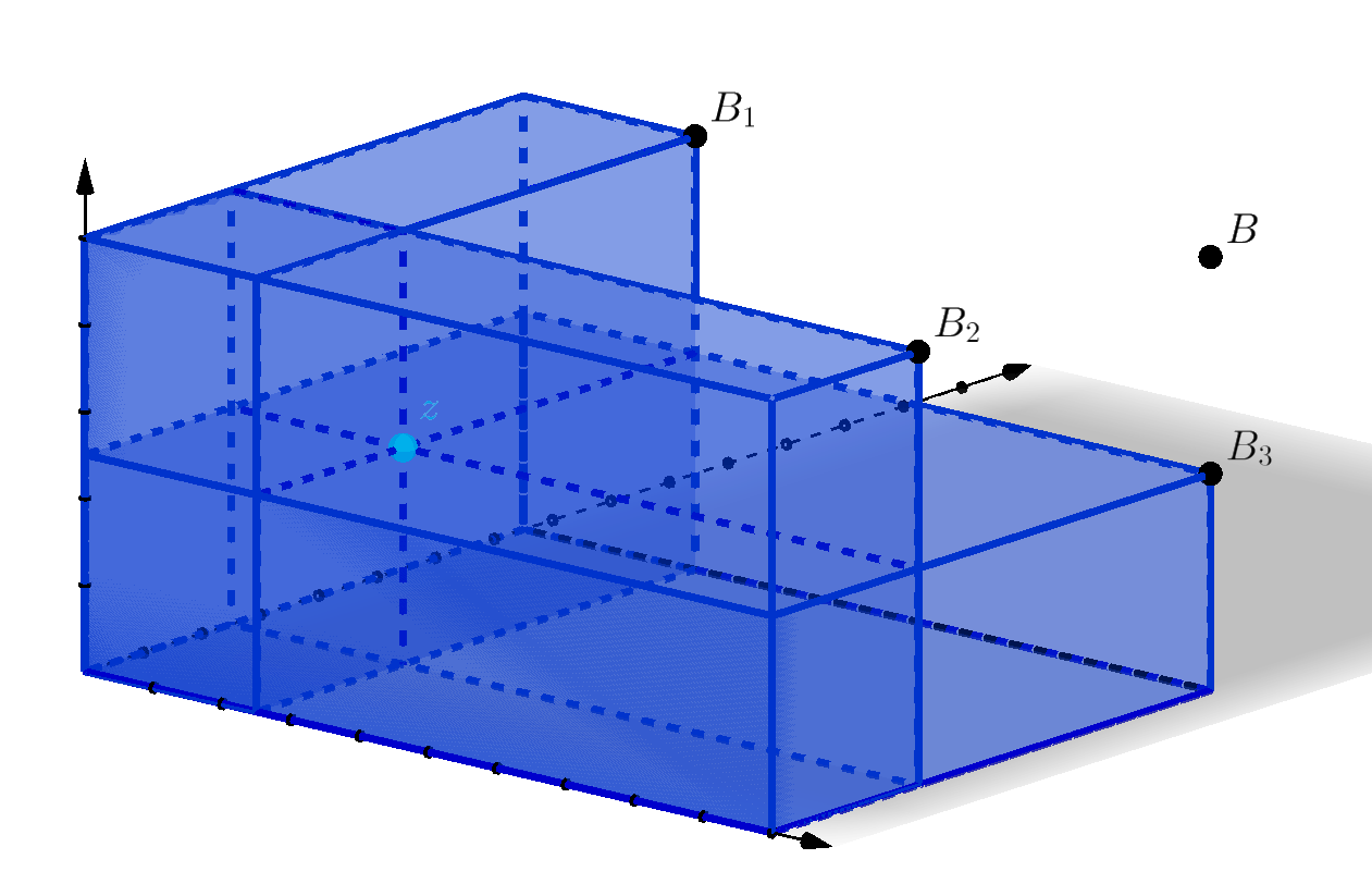
(b) Resulting boxes after full p-split: $\mathbf{B_{1}}=\leavevmode\nobreak\ [(5,15,10)]$, $\mathbf{B_{2}}=\leavevmode\nobreak\ [(20,5,10)]$, and $\mathbf{B_{3}}=\leavevmode\nobreak\ [(20,15,5)]$. All the lower bounds are $(0,0,0)$. Each box shares some space with another box.

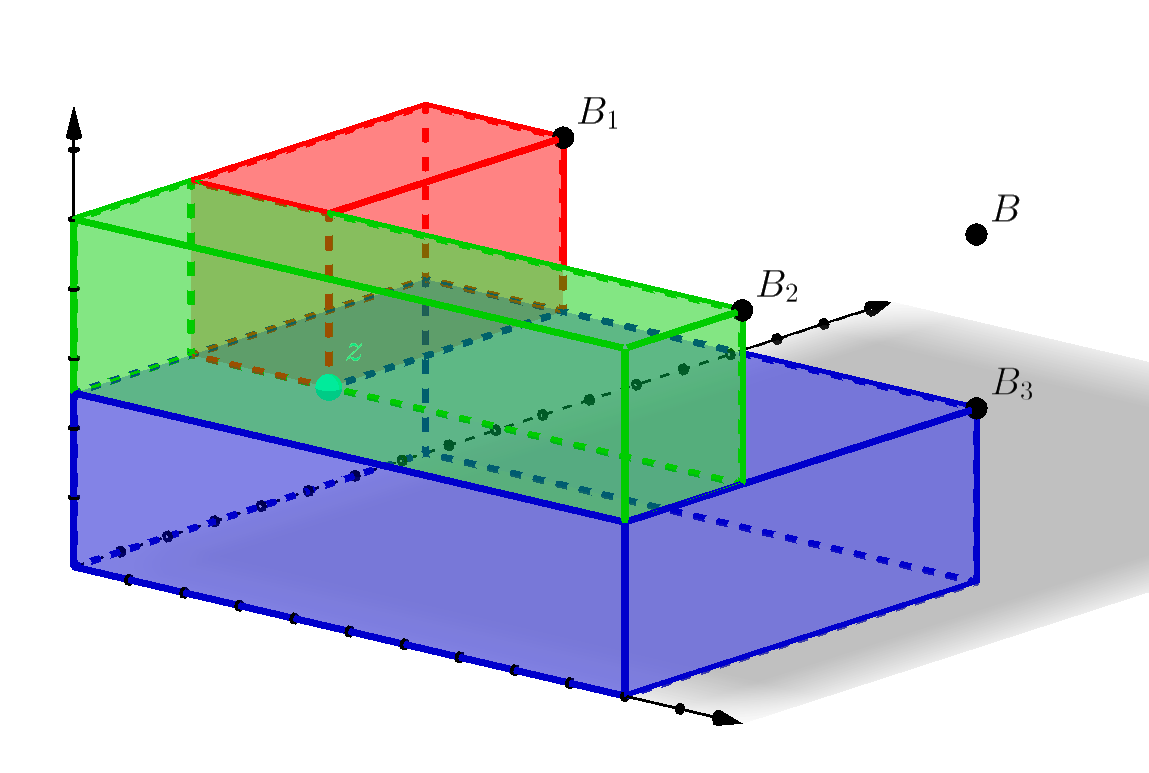
(c) Resulting boxes after p-partition: $\mathbf{B^{*}_{1}}=[(0,5,5),\,(5,15,10)]$, $\mathbf{B^{*}_{2}}$$=[(0,0,5),\,(20,5,10)]$, and $\mathbf{B^{*}_{3}}=[(0,0,0),\,(20,15,5)]$. Each pair of boxes is disjoint.

Figure 1: Splitting a box using full p-split and p-partition. Upper bound for the new boxes is the same in both cases, but lower bounds change.

It is very important to eliminate redundant boxes because, otherwise, the computational execution time grows exponentially. For p-partition, we apply a variant of the redundancy elimination (RE) used in full p-split. In the RE method, when a box $A$ is contained in a box $B$, we eliminate $A$ from the priority queue of boxes to explore. For a deep study of how this method works, see [klamroth2015representation]. Nevertheless, it is not possible to apply this idea to p-partition because the lower bounds of the new boxes differ. We join boxes to save this obstacle.

Definition 3.

Let $A=[l^{a},u^{a}]$ and $B=[l^{b},u^{b}]$ be two boxes with $u^{a}\leq u^{b}$. We define the join box of the two boxes as a new box $C=[l^{c},u^{c}]$, where $l^{c}_{i}=\min\{l^{a}_{i},l^{b}_{i}\}$ and $u^{c}_{i}=u^{b}_{i}$ $\forall i=1,\ldots,p$.

Once we introduce join boxes, we cannot guarantee that all the boxes are pairwise disjoint, but we can confirm that the new box does not exclude non-dominated points. We prove this in the next proposition. The priority of the new box $C$ could be greater than the value of the previous boxes $A$ and $B$. This means that box $C$ will have higher preference to be analyzed in subsequent iterations.

Proposition 2.

With the conditions of Definition 3, it holds that $A\cup B\subset C$, which means that analyzing box $C$ substitutes the analysis of the other two boxes.

Proof.

Let $x\in A\cup B$. If $x\in A$, then $l^{c}_{i}\leq l^{a}_{i}\leq x<u^{a}_{i}\leq u^{b}_{i}=u^{c}_{i}$ $\,\forall i$, so $x\in C$. If $x\in B$, then $l^{c}_{i}\leq l^{b}_{i}\leq x<u^{b}_{i}=u^{c}_{i}$ $\,\forall i$, so $x\in C$. ∎

We are now ready to present in Algorithm 4 the updating procedure of Line 14 in Algorithm 2. It is divided into two parts. In the first part (Lines 1 to 9), the boxes in $\mathfrak{L}$ are split using p-partition. Some of the new boxes may be empty. The non-empty boxes are inserted into the corresponding $\mathfrak{L}_{i}$ according to their direction (Line 6). The priority function used for the boxes is detailed in the next subsection. The second part (Lines 10 to 17) filters the redundant boxes using RE but taking into account that if a domination relation between two upper bounds is detected, the boxes are joined and the new box replaces the older ones (Lines 12 to 15). We finish this subsection proving the correctness and termination of TPA.

Proposition 3.

Algorithm TPA never finds the same non-dominated point twice.

Proof.

Let $B$ be the box being explored in TPA and $z$ the non-dominated point found solving $P(B.u,\omega)$ in Line 11 of Algorithm 2. The definition of the mathematical program $P$ ensures that $z<B.u$, and the use of p-partition with each box $B^{\prime}$ such that $z<B^{\prime}.u$ discards $B^{\prime}_{0}(z)$, which is the only box that can contain $z$. The upper bound of a join box is always the upper bound of a previous box. Thus, after the updating procedure, the remaining boxes do not contain $z$ and $z$ cannot be found again. ∎

Algorithm 4 Update

0:  $(\mathfrak{L},z)$

0:  $(\mathfrak{L},z)$

1:  for all $B\in\bigcup_{k=1}^{p}\mathfrak{L}_{k}$ with $z<B.u$ do

2:     for $i=1$ to $p$ do

3:        $B_{i}(z)=\left\{x\in B\mid x_{i}<z_{i}\text{ and }x_{j}\geq z_{j}\,\forall j>i\right\}$

4:        if $\left(B_{i}(z)\neq\emptyset\right)$ then

5:           $B_{i}(z).priority\leftarrow reduced\_scaled(B,i,z)$

6:           $\mathfrak{L}_{i}.insert(B_{i}(z))$

7:        end if

8:     end for

9:  end for

10:  for $i=1$ to $p$ do

11:     for all $A,B\in\mathfrak{L}_{i}\text{ with }A.u\leq B.u$ do

12:        $C\leftarrow join(A,B)$

13:        $\mathfrak{L}_{i}.remove(A)$

14:        $\mathfrak{L}_{i}.remove(B)$

15:        $\mathfrak{L}_{i}.insert(C)$

16:     end for

17:  end for

Theorem 1.

TPA terminates after finding all the non-dominated points of the MOCO problem if the time limit is not set.

Proof.

The number of non-dominated points is finite in MOCO problems. By Proposition 3, no points are found twice. Thus, TPA terminates. Proposition 2 ensures that all PF is found if enough time is given. ∎

5.3 A new priority function

As the third contribution, we define a new priority function for the boxes. We want to give more priority to boxes having a larger region where non-dominated points can potentially exist. Given a non-empty box $B=[l,u]$, we define the $scaled$ function as

$$scaled(B)=\prod_{i=1}^{p}\left(\frac{u_{i}-l_{i}}{\overline{z}^{N}_{i}-z^{I}_{i}}\right).$$ (15)

Note that $scaled(B)>0$. In the case of an empty box, we define $scaled(B)=0$. We assume, without loss of generality, that $\overline{z}_{i}^{N}>z_{i}^{I}\,\,\forall i$, otherwise the objective $i$ always takes the same value and can be discarded.

In some boxes, there is a region that cannot contain any non-dominated point. In this case, the $scaled$ function overestimates the priority of the box. We define a new priority function to correct this overestimation. First, we need some results.