On the eigenvalues of the harmonic oscillator with a Gaussian perturbation
Abstract
We test the analytical expressions for the first two eigenvalues of the harmonic oscillator with a Gaussian perturbation proposed recently. Our numerical eigenvalues show that those expressions are valid in an interval of the coupling parameter that is greater than the one estimated by the authors. We also calculate critical values of the coupling parameter and several exceptional points in the complex plane.
1 Introduction
Fassari et al[1] studied a harmonic oscillator with a Gaussian perturbation. By means of the Fredholm determinant they derived analytical expressions for the first two eigenvalues. These expressions resemble those commonly obtained by perturbation theory as they are polynomials of second degree in the coupling constant. They showed a figure for these approximate eigenvalues as functions of the coupling constant but did not compare their results with any independent calculation. The purpose of this paper is to test the accuracy of those results and derive some relevant mathematical properties of the eigenvalues of the model.
In section 2 we introduce the model and show some analytical results including the polynomial expressions of Fassari et al[1]. In section 3 we briefly discuss two methods for the calculation of the eigenvalues and related quantities. In section 4 we calculate some critical values of the coupling constant. In section 5 we obtain the exceptional points of the eigenvalues of the model. Finally, in section 6 we summarize the main results and draw conclusions.
2 Analytical expressions
The Hamiltonian operator in the coordinate representation is
| (1) |
Fassari et al[1] considered the cases and separately but it is convenient to treat them in a unified way. Since the potential is parity invariant the solutions to the Schrödinger equation are either even () or odd () so that we can treat the two symmetry species separately. The eigenvalues of decrease with as predicted by the Hellmann-Feynman theorem[2, 3]
| (2) |
By means of a somewhat laborious method Fassari et al[1] obtained
| (3) |
for the two lowest eigenvalues. These expressions show the first two terms of the perturbation expansions[4]
| (4) |
for and (even and odd solutions, respectively). According to the HFT (2) , and the standard equations of perturbation theory[4] show that for and in agreement with equation (3). The perturbation series (4) in general and the analytical expressions (3) in particular are valid for all values of within its radius of convergence. This point is discussed below in section 5.
3 Numerical approaches
The calculation of perturbation terms of greater order can be rather cumbersome. For this reason we resort to two numerical methods.
The first one is the well-known Rayleigh-Ritz (RR) variational method that is based on matrix representations of the Hamiltonian operator in a suitable orthonormal basis [5, 6]. This approach is useful if we can obtain the matrix elements in order to build matrix representations of the form . The approximate eigenvalues are given by the roots of the secular determinant , where is the identity matrix. The advantage of this approach is that the approximate eigenvalues converge towards the exact ones from above: [5, 6]. In the present case we may resort to the well-known basis set of eigenfunctions of and, as argued above, apply the method to even and odd states separately.
The second approach is the Riccati-Padé method (RPM)[7] that has proved to be quite accurate in the past[8, 9] and that is easy to apply to this kind of problems. The starting point of this approach is the logarithmic derivative of the wavefunction , where the prime stands for the derivative with respect to and for even states and for odd ones. The logarithmic derivative can be expanded in a Taylor series about the origin and the approximate eigenvalues are roots of the Hankel determinants , where is the dimension of the determinant and is related to the Padé approximant used in its construction[7, 8, 9].
With both methods we obtain the approximate eigenvalues from the roots of polynomial functions of and . It is clear that we can have either or .
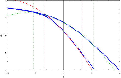
Figure 1 shows the analytical expressions of Fassari et al[1] and present numerical results in the interval . We appreciate that and are reasonably accurate in the intervals and , respectively. A rigorous discussion of this point will be given in section 5. Note that and approach each other as decreases. The reason is that the potential is a double well when and that the barrier between the wells increases as decreases. As the barrier increases pairs of eigenvalues become quasi-degenerate as illustrated in figure 1 for the two lowest ones.
4 Critical values of
For all the eigenvalues are positive. Since they decrease with there may be a value such that for a given value of . The methods introduced above are suitable for this calculation because it is only necessary to obtain the roots of for increasing values of .
In the case of the RR we obtain such that . Since we conclude that (the RR results already exhibit this behaviour). A similar calculation can be carried out with the RPM but this approach does not produce bounds.
From equation (3) we obtain and that agree quite well with the numerical results and . This fact is not surprising because these values of lie within the range of validity of the analytical polynomial expressions as shown in figure 1. In section 5 we provide a more rigorous analysis.
The RPM is suitable for the calculation of extremely accurate results; for example, in this case we obtained
| (5) | |||||
with .
5 Exceptional points
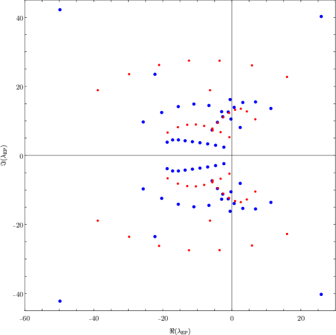
The radius of convergence of the perturbation series (4) is determined by the singularity of closest to the origin of the complex -plane. We can estimate branch points of order two in more than one way. A simple one is based on the discriminant , where is a polynomial of degree [10] (and references therein). This kind of singularities is given by the roots of . Since then we can obtain the singular points by solving the set of equations by means of a root finder like the Newton-Raphson method. In the present paper we use the singular points obtained from the discriminant of the secular determinant provided by the RR method[10] as starting points for the application of the Newton-Rapson method to the set of equations derived from Hankel determinants. The singularities of are commonly called exceptional points (EPS) (see, for example[10] and the references therein). If is the exceptional point of closest to the origin of the complex -plane, then the perturbation series (4) converges for .
Figure 2 shows some of the EPS calculated by means of the RR variational method and the discriminant as discussed in an earlier paper[10]. By means of the RPM with we obtained the following highly accurate results
| (6) | |||||
for the two lowest eigenvalues. In principle, such accuracy is unnecessary for most applications; however, this kind of highly accurate results may be of utility for testing the convergence of new approaches. The radius of convergence for the ground state and first excited state clearly show that the perturbation series (4) are valid for greater intervals of than those estimated by Fassari et al[1]. It is clear that present values of the radii of convergence of the perturbation series provide a rigorous explanation of the results in figure 1 that were discussed in section 3 . Note that figure 1 shows four vertical lines located at and to facilitate the analysis.
6 Conclusions
We have argued that the analytical expressions derived by Fassari et al[1] provide the two lowest corrections of perturbation theory for the two lowest eigenvalues of the harmonic oscillator with a Gaussian perturbation. By means of two independent numerical methods we calculated some critical values of the coupling parameter and also the exceptional points of the eigenvalues of the model. The latter quantities enabled us to determine that the range of validity of the power series (3) is greater that the one estimated by the authors.
References
- [1] S. Fassari, L. M. Nieto, and F. Rinaldi, Eur. Phys. J. Plus 135, 728 (2020).
- [2] P. Güttinger, Z. Phys. 73, 169 (1932).
- [3] R. P. Feynman, Phys. Rev. 56, 340 (1939).
- [4] F. M. Fernández, Introduction to Perturbation Theory in Quantum Mechanics (CRC Press, Boca Raton, 2001).
- [5] J. K. L. MacDonald, Phys Rev. 43, 830 (1933).
- [6] F. M. Fernández, On the Rayleigh-Ritz variational method, https://arxiv.org/abs/2206.05122.
- [7] F. M. Fernández, Q. Ma, and R. H. Tipping, Phys. Rev. A 39, 1605 (1989).
- [8] F. M. Fernández and J. Garcia, Acta Polytechnica 57, 391 (2017).
- [9] F. M. Fernández and J. Garcia, Appl. Math. Comput. 317, 101 (2018).
- [10] P. Amore and F. M. Fernández, Eur. Phys. J. Plus 136, 133 (2021).