An Analytic Description of Electron Thermalization in Kilonovae Ejecta
Abstract
A simple analytic description is provided of the rate of energy deposition by -decay electrons in the homologously expanding radioactive plasma ejected in neutron star mergers, valid for a wide range of ejecta parameters- initial entropy, electron fraction {} and density . The formulae are derived using detailed numerical calculations following the time-dependent composition and -decay emission spectra (including the effect of delayed deposition). The deposition efficiency depends mainly on and only weakly on . The time at which the ratio between the rates of electron energy deposition and energy production drops to , is given by , where , days and . The fractional uncertainty in due to nuclear physics uncertainties is . The result reflects the fact that the characteristic -decay electron energies do not decrease with time (largely due to "inverted decay chains" in which a slowly-decaying isotope decays to a rapidly-decaying isotope with higher end-point energy). We provide an analytic approximation for the time-dependent electron energy deposition rate, reproducing the numerical results to better than 50% (typically , well within the energy production rate uncertainty due to nuclear physics uncertainties) over a 3-4 orders-of-magnitude deposition rate decrease with time. Our results may be easily incorporated in calculations of kilonovae light curves (with general density and composition structures), eliminating the need to numerically follow the time-dependent electron spectra. Identifying , e.g. in the bolometric light curve, will constrain the (properly averaged) ejecta .
keywords:
transients: neutron star mergers – transients: supernovae – nuclear reactions, nucleosynthesis, abundances1 Introduction
The violent merger of two neutron stars (or a neutron star and black hole) has been predicted to produce high-density neutron-rich ejecta, in which heavy elements beyond Iron are formed via the -process (Lattimer & Schramm (1974), see Shibata & Hotokezaka (2019); Radice et al. (2020); Rosswog & Korobkin (2024) for recent reviews). The radioactive decay of these freshly synthesized, unstable -process nuclei should power an optical transient (Li & Paczyński, 1998) commonly referred to as a "kilonova" (see Fernández & Metzger (2016); Nakar (2020); Margutti & Chornock (2021) for recent reviews). The observed UV-IR emission following the neutron star merger event GW170817 (Arcavi et al., 2017; Coulter et al., 2017) is broadly consistent with these predictions (Drout et al. (2017); Hotokezaka et al. (2018); Kasen et al. (2017); Kasliwal et al. (2017); Waxman et al. (2018)), confirming the existence of an -process powered transient with and characteristic velocity . (Cowperthwaite et al., 2017; Kasen et al., 2017; Tanaka et al., 2017; Tanvir et al., 2017; Rosswog et al., 2018). Nonetheless, an outstanding problem in kilonovae analysis is the translation of kilonovae observations to robust constraints on the ejecta properties, in particular on the -process nucleosynthesis and on the final ejecta composition.
Interpreting kilonovae observations requires understanding the processes by which secondary particles produced in radioactive decay deposit energy, i.e., “thermalize,” in the ejected plasma. Radioactivity produces energetic particles (photons, electrons, alphas, and fission fragments). Initially, the particles’ energy is wholly absorbed in the plasma. However, as the ejecta expand and dilute, the energy is only partially absorbed, leading to an energy deposition rate that deviates from the total energy release rate. -rays initially dominate the radioactive heating, up to day at which time they escape the plasma (Barnes et al., 2016; Guttman et al., 2024). On a timescale of days, the main heating source is expected to be -decay electrons, with possible and fission heating contributions depending on initial and nuclear mass model: For initial , -decay electron heating is expected to dominate the heating for all day, with a possible comparable contribution from fission heating at days for some nuclear mass models (e.g Zhu et al., 2021); For initial , mass model uncertainties yield larger variance in the heating contributions- -particle heating was found to be of the same order as -decay electron heating for days for some mass models (e.g. Zhu et al., 2021; Barnes et al., 2021) and fission fragments may be equally important on timescales of for most mass models investigated (However, the fission contribution is highly uncertain due to uncertainties in theoretical mass models, fission barriers, and fission rates, e.g. Zhu et al., 2021; Barnes et al., 2021). Therefore, notwithstanding the effects of fission, late-time kilonovae light-curve interpretation requires an understanding of the inefficient thermalization timescale on which electrons efficiently deposit their energy, particularly for compositions with initial .
In this work, we calculate the time-dependent energy deposition rate per unit mass, , by electrons and positrons (in what follows, we refer to both as "electrons") emitted by -decays in homologously expanding plasma ejected in binary neutron star (BNS) mergers for a wide range of ejecta parameters, . Using detailed numeric nucleosynthesis calculations, we obtain the time-dependent composition, stopping power, and -decay energy spectra, and follow the evolution of the electron energy distribution, assuming that the electrons are confined by magnetic fields to the fluid element within which they were produced111 Magnetic confinement appears likely since it would be facilitated by a relatively weak magnetic field. Assuming in the expanding ejecta, as may be appropriate for a tangled field, G is expected at days, cm (the equipartition field at 10 days is mG), implying an electron Larmor radius of cm. (i.e., including "delayed energy deposition", the deposition at time by electrons that were emitted at and did not lose all their energy by the time ). The secondary electrons that are ionized by -decay electrons have very low kinetic energies and thermalize rapidly, we thus assume that they fully thermalize upon emission. Finally, we test the sensitivity of our results to uncertainties in nuclear physics.
We carry out calculations over a broad range of values of ejecta parameters , that generously covers the expected ejecta parameter range from binary neutron star merger simulations (e.g. Radice et al., 2018; Nedora et al., 2021) : , where is our benchmark value motivated by the inferred mass and characteristic velocity of the ejecta of GW170817 (Drout et al., 2017; Hotokezaka et al., 2018; Kasen et al., 2017; Kasliwal et al., 2017; Waxman et al., 2018) (for homologous expansion, is a constant of the ejecta determined by its mass and velocity spread); ; . Our results may be readily applied to ejecta with general density and composition structures by properly integrating over the ejecta components. Under the assumption that electrons are confined to the plasma by magnetic fields, such integration would be valid also at late times, , at which delayed deposition may become important.
We provide a simple analytic description of the thermalization efficiency that is valid for a wide range of ejecta parameters, {, }, extending the results of earlier works, that compile tables of parameterized fits to the thermalization efficiency for specific combinations of ejecta mass and velocity (e.g. Barnes et al., 2016). Although our calculated values are broadly consistent with those of earlier works (Metzger et al., 2010; Barnes et al., 2016; Hotokezaka & Nakar, 2020; Kasen & Barnes, 2019), our analytic approximation differs from earlier analytic results. This is partly due to our calibration against a systematic numeric analysis, and partly due to assumptions adopted in earlier work, which we find invalid (see § 4). In particular, it is commonly assumed that the characteristic energy of electrons released in -decays drops with time (e.g. Kasen & Barnes, 2019; Hotokezaka & Nakar, 2020), leading to a dependence of on which is stronger than the scaling expected for time-independent characteristic energy (see discussion in § 4.2). While the -value of -decays decreases with decay half-time , this does not imply (as pointed out in Waxman et al., 2019) a decrease of the characteristic -decay electron energy with time , since there is a very large spread in the relation between and and since the decay of an isotope with a low -value and a long lifetime may produce an unstable isotope with a short lifetime and a high -value. We find here that such "inverted decay chains" lead to a nearly time-independent, or slightly rising with time, characteristic -decay electron energy, and with .
The plasma stopping power depends on the ejecta composition and on the energy spectrum of the -decay electrons, which in turn depend on (and ). is therefore often expected to depend strongly on and nuclear physics inputs (Barnes et al., 2016; Barnes et al., 2021; Zhu et al., 2021). We find that the deposition efficiency, particularly , depends primarily on , with only a weak dependence on and on nuclear physics uncertainties. This is due to the fact that the ionization stopping power. which dominates the energy loss, depends on the composition mainly through the ratio of atomic number and mass, , which is nearly composition independent, and since the characteristic -decay electron energy depends weakly on composition.
This paper is organized as follows. In § 2, we describe our nucleosynthesis and electron spectra calculations. In § 3, we give the equations we used for (numerically) calculating the electron energy loss and deposition, and the definition of . § 4 presents our results. In § 4.1 we present our analytical formulae for . In § 4.2 we discuss the characteristic energy of -decay electrons. In § 4.3 we present our analytical formulae for the energy deposition rate . § 4.4 presents an analysis of the sensitivity of our results to nuclear physics uncertainties. We summarize and discuss our conclusions in § 5.
2 Nucleosynthesis and Electron Spectra Calculation
We carry out nucleosynthesis calculations over a 129 grid of {,} values, with logarithmic spacing in , semi-linear spacing in , and linear spacing in . BNS merger simulations show that most dynamical ejecta and secular wind ejecta have an entropy , while a small mass fraction of the dynamical ejecta () has (Radice et al., 2018; Nedora et al., 2021).
We compute time-dependent yield abundances using the publicly available SkyNet nuclear network, including 7843 isotopes up to (Lippuner & Roberts, 2017). SkyNet requires time-dependent trajectories of Lagrangian fluid elements to predict the temporal evolution of the abundances. Matter density evolves first through an exponential phase which is largely constant, before transitioning to a homologous expansion (Lippuner & Roberts, 2015):
| (1) |
where is the expansion timescale of the ejecta. NSE is assumed to hold until , at which time SkyNet switches to a full network evolution. Most works that examine SkyNet nucleosynthesis yields initialize the calculation with given (Perego et al., 2022; Lippuner & Roberts, 2015), where is the initial temperature of the ejecta. For these given values, the EoS determines the initial density (see Lippuner & Roberts (2017) regarding EoS and NSE solver used by SkyNet) and then uses the density history provided by Eq. (1) to evolve the network.
In contrast, we initialize our nucleosynthesis calculations as follows: All runs are initialized with GK, as NSE is expected for this temperature. We supply initial values of , and then find using SkyNet’s EoS solver. We determine from using Eq. (1), such that the ejecta has the desired value. We stress that in this approach is not a meaningful physical parameter; we assume that the ejecta has a particular , and was initially in NSE, in which case specifies the time before expansion. Initializing with different would result in a different , however as NSE conditions hold for both, the same composition is achieved. This alternative approach allows us to directly probe the dependence on for fixed within the range obtained in BNS simulations.
We employ the latest JINA REACLIB database (Cyburt et al., 2010), with specific corrections as described in Appendix B of Guttman et al. (2024), using the same setup as in Lippuner & Roberts (2015) for the other input nuclear physics. More specifically, strong inverse rates are computed assuming detailed balance. Spontaneous and neutron-induced fission rates are taken from Frankel & Metropolis (1947); Panov & Janka (2009), adopting fission barriers and fission fragment distributions from Mamdouh et al. (2001); Wahl (2002). Nuclear masses are taken from the REACLIB database, which includes experimental masses and theoretical masses calculated from the FRDM model (Möller et al., 2016).
We use experimental data from the latest ENDF database (Brown et al., 2018) to calculate the time-dependent energy released in electrons. We ensure that the total energy release we compute is equivalent to as calculated by SkyNet. We use BetaShape (Mougeot, 2017) to calculate spectra of individual -decays. We then compute the full time-dependent emission spectra using the calculated activities of -decaying isotopes.
3 Radioactive Heating
In this section, we first present the energy-loss mechanisms for electrons, and then describe the energy deposition calculation method and the definition of .
3.1 Electron energy loss
-decay electrons emitted in the MeV range lose energy primarily through ionization losses. However, for initial entropies , the ejecta composition is dominated by H and/or He (Perego et al., 2022). In this case, plasma losses dominate over other energy loss mechanisms.
We calculate mass-weighted, time-dependent stopping powers based on the instantaneous composition of the ejecta,
| (2) |
Where is the energy loss per unit column density for a particular isotope, is the isotope’s mass number and is its number fraction, defined such that . For electron ionization losses, we use (Longair, 2011)
| (3) |
where is the energy loss per unit column density traversed by the electron, , is the electron’s velocity, is the Lorentz factor of the electron, and are the atomic and mass numbers of the plasma nuclei, and is the effective average ionization potential which can be approximated for an element of atomic number Z as (Segre, 1977): eV.
For plasma losses, we use (Solodov & Betti, 2008)
| (4) |
where is the number of free electrons per atom, is the plasma frequency, and is the number density of free electrons. We use and eV (we keep fixed at this value since it affects the stopping power only logarithmically).
Finally, at highly relativistic energies, Bremsstrahlung losses significantly contribute to electron losses (Longair, 2011)
| (5) |
Figure 1 shows the electron stopping power contributions for Xe composition.

3.2 Electron Energy Deposition
3.2.1 Deposition Equations
The energy deposited by electrons at time is given by
| (6) |
where is the number of electrons per unit energy, determined by the continuity equation in energy space
| (7) |
Here, is the number of electrons released per time per unit energy (as determined from the time-dependent abundances), and is the full energy-loss rate for electrons, given by
| (8) |
The first term on the right-hand side accounts for adiabatic energy losses and the second term accounts for energy transferred to the plasma as described in § 3.1. The adiabatic losses are obtained assuming that the high-energy electrons behave as an ideal gas, in which case we have for highly relativistic electrons and in the highly non-relativistic limit. -decay electrons are mildly relativistic, with , and as they lose energy, the value of that best describes the evolution is changing. We take a fixed throughout all our calculations. We numerically solve Eq. (7) for and use the result in order to integrate Eq. (6).
3.2.2 Instantaneous Deposition and
We define the fraction of energy instantaneously deposited at time as
| (9) |
where is the energy production rate in -decay electrons, and the fraction of energy instantaneously deposited by an electron produced at time with energy is approximated as
| (10) |
Here is the deposition energy loss timescale. Under this approximation, deposition deviates from full efficiency when the deposition energy loss timescale becomes larger than the dynamical time . Note that at late times because . is defined as
| (11) |
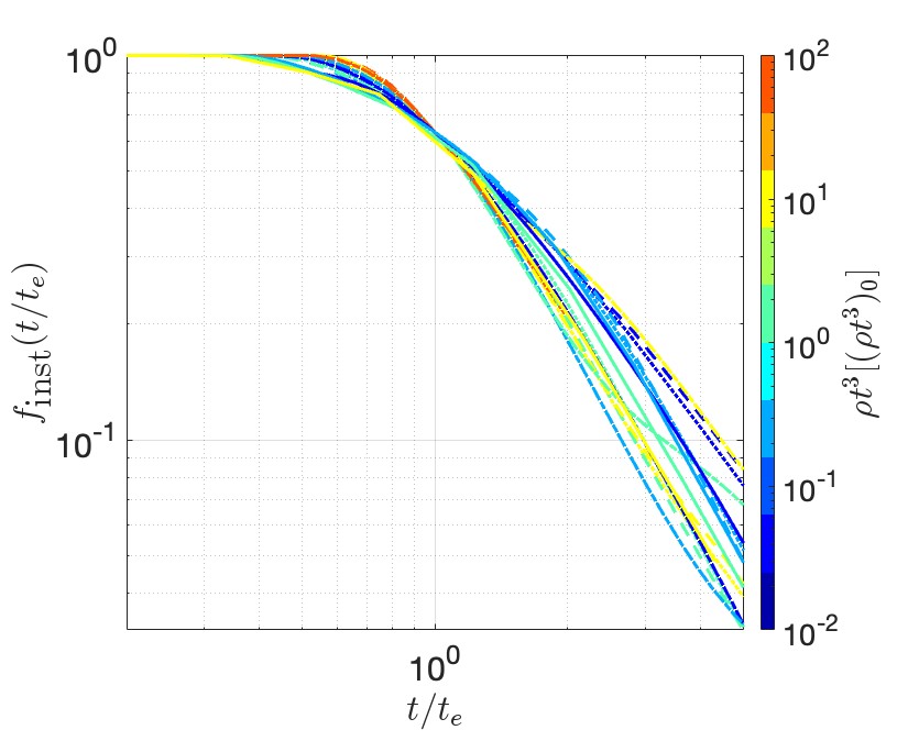
In Figure 2 we plot for different ejecta parameters. At late times approaches a behavior, as expected from Eq. (10), although deviations from this behavior may occur due to variations in the emitted electron spectra. The rather common behavior of instantaneous deposition for different ejecta parameters suggests that an approximate analytic description may be obtained.
In Figure 3, we compare the rate of electron energy release and deposition. At early times, when , . This is due to energy that is lost to adiabatic expansion (first term on right-hand side of Eq. (8)). At , , with the exact factor depending on ejecta parameters. We are therefore confident in using our definition of as the inefficient deposition timescale, even though it is defined with respect to instantaneous deposition. At , as delayed deposition starts to dominate. At , regardless of , as was obtained analytically in Waxman et al. (2019).
4 Analytic approximations and nuclear physics uncertainties
4.1 Analytical approximation for
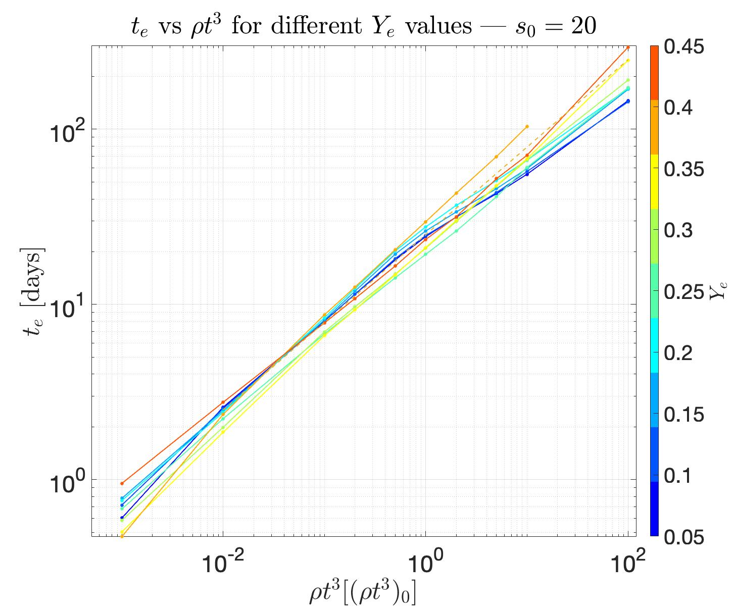
In Figure 4, we plot vs. for a range of values (and ), together with a fit. It is clear that the depends primarily on and that a power-law fit is appropriate. However, there is a secondary dependence. Particularly, for , drops below the curve for . We find that serves as the breakpoint for a broken power-law description of for different combinations of and . Therefore, we suggest the following broken-power law description
| (12) |
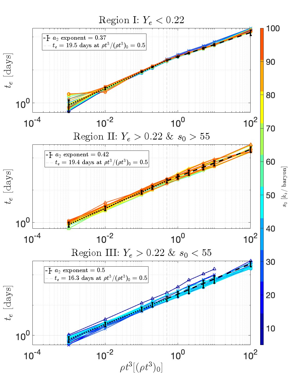
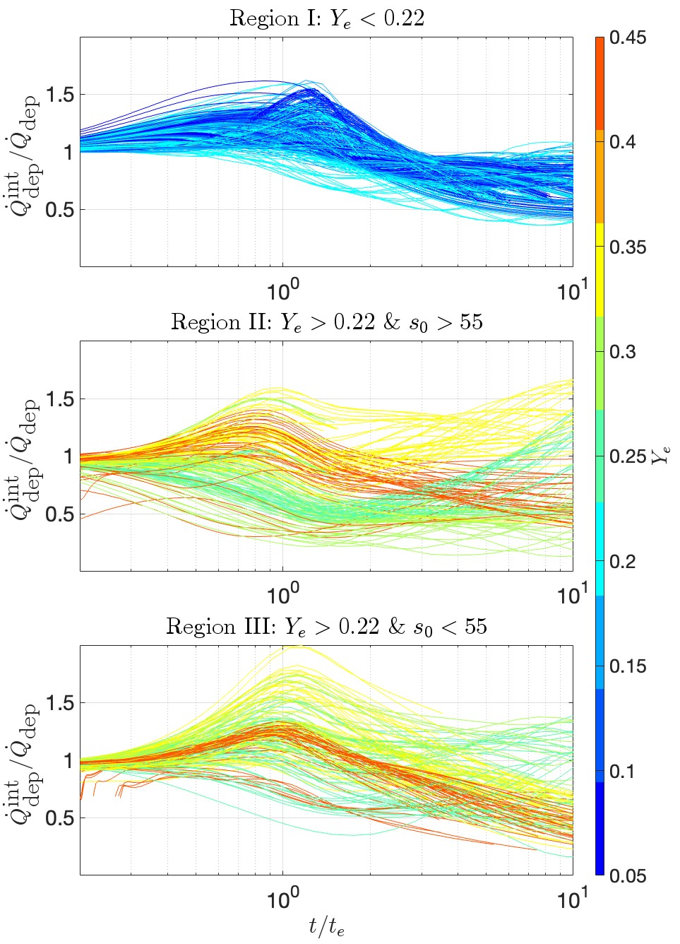
In Figure 5, we plot (as obtained from a fit of the numeric result to Eq. (12) as a function of and . We identify 3 regions within which similar values of are obtained: Region I - ; Region II - & ; Region III - & . Nucleosynthesis calculations predict the production of 3rd-peak r-process elements in Region I (e.g Perego et al., 2022), post 1st-peak elements in Region II (with 2nd-peak elements created for ), and elements up to in Region III.

Table 1 presents the best-fit parameters for Eq. (12) for the 3 regions considered. In Figure 6 we plot for all three regions, together with their respective broken power-law fits from Table 1. Error bars show the standard error of the estimate, defined as where is the value of the fit, calculated according to Eq. (12), and is calculated according to Eq. (11) for the different and values considered. The fit for Region I exhibits the best uniformity, with a fractional standard error (defined as ) of for all values excluding , for which . For Regions II and III, , with the exact value depending on the value of .
We find that for our entire parameter space, while for Regions I, II and III, respectively. As noted in the introduction, the fact that the power-law indices are close to implies that the characteristic energy of the -decay electrons does not vary significantly with time, and the lower than values suggest a minor increase in this energy with time. We discuss this further in § 4.2.
4.2 The characteristic energy of -decay electrons
The relation between the dependence of on and the dependence of the characteristic -decay electron energy on time may be qualitatively understood as follows. is approximately the time at which the expansion time, , equals the deposition (mainly by ionization) energy loss time, where is the initial electron energy. Noting that is only weakly dependent on energy at the relevant energy range (see Figure 1),
| (13) |
and
| (14) |
For characteristic -decay electron energy that varies with time as , we have .
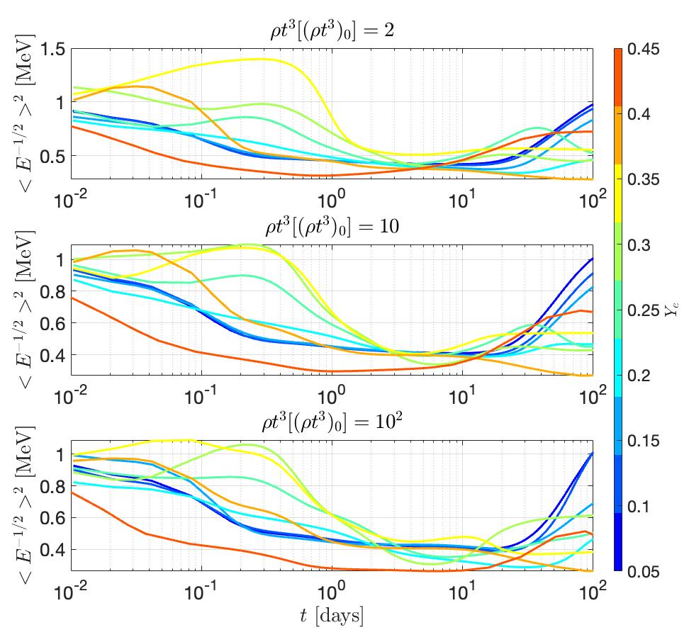
Figure 7 shows the characteristic -decay energies vs. time for several values (with ). Motivated by Eq. (14), we define the characteristic energy as , rather than , where the brackets denote an average over the electron energy spectra (weighted by the electron energy). Several conclusions may be drawn from this figure. Firstly, only for does the characteristic energy monotonously decrease with time up until days. This is consistent with Figure 4, where only the curve exhibits a logarithmic slope (of the dependence of on ) that is at late times. For , we see a sharp rise in characteristic energy around days. For these values, we find that the radioactive heating at days becomes dominated by the following decay-chain
| (15) |
This is an example of an "inverted decay-chain" in which a slowly decaying isotope decays to a rapidly decaying isotope with higher energy release. We find that at these times, other inverted decay-chains are also active and contribute significantly to the heating. These include and others, depending on . We note that these occur only for even values of , and may be understood using the semi-empirical mass formula (Weizsäcker, 1935). The pairing term in the formula creates two mass parabolas for a given : one for even-even and another for odd-odd nuclei. As the nucleus decays, it transitions between these parabolas, resulting in uneven energy releases until reaching stability. Overall, there are 40 inverted decay-chains for which a slowly decaying isotopes decays into a rapidly decaying isotopes with half-life of its parent isotope, 26 of these are for decay chains with .
In Region I ( & , see Table 1), third peak process elements are robustly produced. Therefore, the inverted decay chains for are active, leading to an increase in late-time characteristic energy release and, thus, a lower value of the exponent, . In Region II, the situation is more subtle. We note that in NSE, the entropy scales monotonically with the photon-to-baryon ratio . The abundance of an isotope () in NSE is proportional to and thus NSE with high entropy favors more free neutrons and less heavy-nuclei (Meyer, 1993). As the ejecta expand and exit NSE, the many free neutrons are captured on the few seed nuclei, leading to heavy-element production. Thus for , third peak elements are produced, albeit less than in Region I by a factor , despite the ejecta being relatively neutron-poor. The inverted decay chains for are similarly active. For , -process elements are produced up to the second peak (up to ). Despite the high entropy, the ejecta is too neutron-poor to create second and third-peak -process elements. For these values of in Region II, the inverted decay chains for dominate the heating from days, leading to an increase in characteristic initial electron energy. For these same high values but for low values of (Region III), isotopes up to are synthesized, and thus, none of the significant inverted decay chains are active. In Region III, the characteristic initial electron energy, for the most part, either stays constant or slightly declines over time, yielding as is expected from Eq. (14).
We conclude that inverted -decay chains are not insignificant anomalies that can be disregarded when considering characteristic energies of -decay electrons. Their presence in nearly all the nucleosynthesis runs considered, especially those with significant heavy element production, invalidates the assumption that the characteristic electron energy steadily declines with time.
4.3 Analytic approximation for
In this section we provide an interpolating function that describes the electron energy deposition rate both at early () and late () times, for different values of . Since at late times regardless of (see Waxman et al. (2019)), we provide an interpolation for rather than for the fractional deposition, . We suggest the following interpolation:
| (16) |
Here, are free parameters to be fitted for and is given by Eq. (12). governs the transition from the early-time to late-time interpolation. governs the shift from full to partial deposition until . governs the late-time asymptotic deposition, which should approach a behavior. is the time at which the delayed deposition overtakes the instantaneous deposition, and should be roughly . The first term in ensures that for such that interpolates correctly between the early/late-time regimes.
We fit values for the three different regions in as described in § 4.1. Our fitting employed a gradient descent over these four parameters while minimizing the cost function defined as , where , are logarithmically spaced from up to . The best-fit parameters are compiled in Table 1. The values obtained for and are , as is expected for the correction transition to the late-time asymptotic heating.
In Figure 8, we compare and for the same sample of parameters as shown in Figure 3. In Figure 9 we check the accuracy of the analytic description of for all nucleosynthesis parameters considered. Our interpolation is most accurate in Region I, within which the nucleosynthesis yield is mostly uniform. In Regions II and III, different parameters result in different nucleosynthesis yields, and therefore different deposition curves, which reduces the accuracy of the fit. The quality of the fit and its spread may be gauged by considering the standard deviation of at each time, for each region. Averaging the standard deviation over logarithmic time for each region, we find that for Regions I, II, and III, respectively. Overall, our interpolation is nearly accurate to within over orders-of-magnitude change in for our entire parameter space. Note that Eq. (12, 16) provide an analytic description that requires as input in order to determine the full electron deposition up to .

| Ejecta Parameters | Power-Law Parameters | Interpolation Parameters | |||||||
| [days] | m | ||||||||
| Region I | 0.5 | 0.37 | 19.5 | 4.5 | 1.1 | 2.8 | 1.3 | ||
| Region II | 0.5 | 0.42 | 19.4 | 0.8 | 0.5 | 2.5 | 1.3 | ||
| Region III | 0.5 | 0.5 | 16.3 | 1.5 | 0.5 | 2.8 | 1.3 | ||
4.4 Nuclear Physics Robustness Checks

Modeling -process nucleosynthesis from BNS mergers requires calculating nuclear masses and nuclear reaction rates for which no experimental data are available. For , different nuclear mass models may result in orders-of-magnitude differences in final composition of post 1st-peak elements () and up to an order-of-magnitude difference in radioactive energy release (Mumpower et al., 2016; Zhu et al., 2021; Barnes et al., 2021). In this section we study the sensitivity of our results to the nuclear physics models’ uncertainties.
To gauge the impact of these uncertainties, we reran our calculations for two different nuclear mass models together with randomized nuclear rates. We edited our local REACLIB file which contains all the rates and cross-sections that go into SkyNet. We modify every strong or weak theoretical interaction rate to
| (17) |
where was randomly chosen from a uniform distribution in . This amounts to changing 70,000 rates (approximately 90% of all rates included). With our new reaction rates file, we reran for a subset of initial parameters: , , for both FRDM and UNEDF1 (Kortelainen et al., 2012, http://massexplorer.frib.msu.edu,) mass models. We repeat the above process 100 times and calculate for each run and compare the values obtained to our nominal values, presented in Figures 4. We stress that these changes lead to orders-of-magnitude differences in final composition between different runs.
In Figure 10, we show histograms of for different values of and , where is calculated according to Eq. (11) for each SkyNet run with randomized reaction rates using both FRDM and UNEDF1 mass models. We see that the mean falls at for all parameter values considered. The spread in values is small, with an average fractional standard deviation of for . For , the spread is even smaller, with .
These tests demonstrate that our results are only weakly sensitive to nuclear physics uncertainties. Different nuclear mass models and different reaction rates may lead to large variations in composition and heating rates. However, these changes do not significantly affect the inefficient thermalization timescales. In retrospect, this was to be expected - Figure 4 shows that is relatively insensitive to the value and thus to the detailed electron energy spectra and ejecta composition.
5 Conclusions
We calculated the time-dependent energy deposition rate per unit mass, (see Eq. (6)), by electrons (and positrons) emitted by -decays in homologously expanding ejecta produced in BNS mergers for a wide range of ejecta parameters, . Using detailed numeric nucleosynthesis calculations, we obtained the time-dependent composition, stopping power, and -decay energy spectra, and followed the evolution of the electron energy distribution, assuming that the electrons are confined by magnetic fields to the fluid element within which they were produced (see Eq. (8)).
The deposition efficiency, the ratio between the rates of instantaneous electron energy deposition and energy production rates, Eq. (10), depends mainly on and only weakly on . , the time at which drops to , is well described by a broken power-law, , see Eq. (12) and Figure 6, with days, and (see Table 1 for exact values). The accuracy of the analytic approximation is within .
The result reflects the fact that contrary to naive expectations, the characteristic energy of the -decay electron spectrum does not decrease with time (see Eq. (14)). This is largely due to "inverted decay chains" in which a slowly-decaying isotope decays to a rapidly-decaying isotope with higher end-point energy. A detailed discussion of the relevant decay chains at different {} values is given in § 4.2. We find that inverted decay chains play a significant role at days, affecting the thermalization timescale at all relevant {} values.
Using our analytic results for , we provided an analytic description of the energy deposition of -decay electrons (and positrons), given by Eq. (16) and Table 1. Our formulae provide an analytic description of the thermalization efficiency, which we find to be only weakly sensitive to (see § 4.1, 4.2, and Figures 4 , 5 , 6) and nuclear physics uncertainties (see § 4.4, Figure 10). This enables one to determine for a given total radioactive energy release rate, . Our analytic description reproduces the numerical results to better than (typically ) accuracy up to , over a orders-of-magnitude deposition rate decrease (see § 4.3, Figures 8 , 9).
In contrast to previous works that compile tables of parameterized fits for the thermalization of specific combinations of ejecta mass and velocity in a specific velocity structure (e.g. Barnes et al. (2016)), we provide a simple analytic description that can be utilized for a wide range of ejecta parameters and density profiles. Our results may thus be easily incorporated in calculations of kilonovae light curves (with general composition, density and velocity structures), eliminating the need to follow the time-dependent electron spectra numerically.
The weak dependence of the deposition efficiency on and on nuclear physics uncertainties implies that identifying in the bolometric kilonova light curve will constrain the (properly averaged) ejecta .
Acknowledgements
BS would like to thank Tal Wasserman for helpful discussions.
Data Availability
Numerical results are available upon request.
References
- Arcavi et al. (2017) Arcavi I., et al., 2017, Nature, 551, 64
- Barnes et al. (2016) Barnes J., Kasen D., Wu M.-R., Martínez-Pinedo G., 2016, The Astrophysical Journal, 829, 110
- Barnes et al. (2021) Barnes J., Zhu Y. L., Lund K. A., Sprouse T. M., Vassh N., McLaughlin G. C., Mumpower M. R., Surman R., 2021, The Astrophysical Journal, 918, 44
- Brown et al. (2018) Brown D., et al., 2018, Nuclear Data Sheets, 148, 1
- Coulter et al. (2017) Coulter D. A., et al., 2017, Science, 358, 1556
- Cowperthwaite et al. (2017) Cowperthwaite P. S., et al., 2017, The Astrophysical Journal, 848, L17
- Cyburt et al. (2010) Cyburt R. H., et al., 2010, The Astrophysical Journal Supplement Series, 189, 240
- Drout et al. (2017) Drout M. R., et al., 2017, Science, 358, 1570
- Fernández & Metzger (2016) Fernández R., Metzger B. D., 2016, Annual Review of Nuclear and Particle Science, 66, 23
- Frankel & Metropolis (1947) Frankel S., Metropolis N., 1947, Physical Review, 72, 914
- Guttman et al. (2024) Guttman O., Shenhar B., Sarkar A., Waxman E., 2024, The thermalization of -rays in radioactive expanding ejecta: A simple model and its application for Kilonovae and Ia SNe
- Hotokezaka & Nakar (2020) Hotokezaka K., Nakar E., 2020, The Astrophysical Journal, 891, 152
- Hotokezaka et al. (2018) Hotokezaka K., Beniamini P., Piran T., 2018, International Journal of Modern Physics D, 27, 1842005
- Kasen & Barnes (2019) Kasen D., Barnes J., 2019, The Astrophysical Journal, 876, 128
- Kasen et al. (2017) Kasen D., Metzger B., Barnes J., Quataert E., Ramirez-Ruiz E., 2017, Nature, 551, 80
- Kasliwal et al. (2017) Kasliwal M. M., et al., 2017, Science, 358, 1559
- Kortelainen et al. (2012) Kortelainen M., McDonnell J., Nazarewicz W., Reinhard P.-G., Sarich J., Schunck N., Stoitsov M. V., Wild S. M., 2012, Physical Review C, 85, 024304
- Lattimer & Schramm (1974) Lattimer J. M., Schramm D. N., 1974, The Astrophysical Journal, 192, L145
- Li & Paczyński (1998) Li L.-X., Paczyński B., 1998, The Astrophysical Journal, 507, L59
- Lippuner & Roberts (2015) Lippuner J., Roberts L. F., 2015, The Astrophysical Journal, 815, 82
- Lippuner & Roberts (2017) Lippuner J., Roberts L. F., 2017, The Astrophysical Journal Supplement Series, 233, 18
- Longair (2011) Longair M. S., 2011, High Energy Astrophysics. https://ui.adsabs.harvard.edu/abs/2011hea..book.....L
- Mamdouh et al. (2001) Mamdouh A., Pearson J. M., Rayet M., Tondeur F., 2001, Nuclear Physics A, 679, 337
- Margutti & Chornock (2021) Margutti R., Chornock R., 2021, Annual Review of Astronomy and Astrophysics, 59, 155
- Metzger et al. (2010) Metzger B. D., et al., 2010, Monthly Notices of the Royal Astronomical Society, 406, 2650
- Meyer (1993) Meyer B. S., 1993, Physics Reports, 227, 257
- Mougeot (2017) Mougeot X., 2017, EPJ Web of Conferences, 146, 12015
- Mumpower et al. (2016) Mumpower M., Surman R., McLaughlin G., Aprahamian A., 2016, Progress in Particle and Nuclear Physics, 86, 86
- Möller et al. (2016) Möller P., Sierk A. J., Ichikawa T., Sagawa H., 2016, Atomic Data and Nuclear Data Tables, 109-110, 1
- Nakar (2020) Nakar E., 2020, Physics Reports, 886, 1
- Nedora et al. (2021) Nedora V., et al., 2021, The Astrophysical Journal, 906, 98
- Panov & Janka (2009) Panov I. V., Janka H.-T., 2009, Astronomy & Astrophysics, 494, 829
- Perego et al. (2022) Perego A., et al., 2022, The Astrophysical Journal, 925, 22
- Radice et al. (2018) Radice D., Perego A., Hotokezaka K., Fromm S. A., Bernuzzi S., Roberts L. F., 2018, The Astrophysical Journal, 869, 130
- Radice et al. (2020) Radice D., Bernuzzi S., Perego A., 2020, Annual Review of Nuclear and Particle Science, 70, 95
- Rosswog & Korobkin (2024) Rosswog S., Korobkin O., 2024, Annalen der Physik, 536, 2200306
- Rosswog et al. (2018) Rosswog S., Sollerman J., Feindt U., Goobar A., Korobkin O., Wollaeger R., Fremling C., Kasliwal M. M., 2018, Astronomy & Astrophysics, 615, A132
- Segre (1977) Segre E., 1977, Nuclei and Particles. An Introduction to Nuclear and Subnuclear Physics. Second edition. W. A. Benjamin, Redwood City, Ca, https://www.biblio.com/book/nuclei-particles-introduction-nuclear-subnuclear-physics/d/1464581338
- Shibata & Hotokezaka (2019) Shibata M., Hotokezaka K., 2019, Annual Review of Nuclear and Particle Science, 69, 41
- Solodov & Betti (2008) Solodov A. A., Betti R., 2008, Physics of Plasmas, 15, 042707
- Tanaka et al. (2017) Tanaka M., et al., 2017, Publications of the Astronomical Society of Japan, 69, 102
- Tanvir et al. (2017) Tanvir N. R., et al., 2017, The Astrophysical Journal Letters, 848, L27
- Wahl (2002) Wahl A., 2002, Technical report, Systematics of Fission-Product Yields. United States
- Waxman et al. (2018) Waxman E., Ofek E. O., Kushnir D., Gal-Yam A., 2018, Monthly Notices of the Royal Astronomical Society, 481, 3423
- Waxman et al. (2019) Waxman E., Ofek E. O., Kushnir D., 2019, The Astrophysical Journal, 878, 93
- Weizsäcker (1935) Weizsäcker C. F. v., 1935, Zeitschrift für Physik, 96, 431
- Zhu et al. (2021) Zhu Y. L., Lund K. A., Barnes J., Sprouse T. M., Vassh N., McLaughlin G. C., Mumpower M. R., Surman R., 2021, The Astrophysical Journal, 906, 94