Multifidelity linear regression for scientific machine learning from scarce data

Abstract

Machine learning (ML) methods, which fit to data the parameters of a given parameterized model class, have garnered significant interest as potential methods for learning surrogate models for complex engineering systems for which traditional simulation is expensive. However, in many scientific and engineering settings, generating high-fidelity data on which to train ML models is expensive, and the available budget for generating training data is limited. ML models trained on the resulting scarce high-fidelity data have high variance and are sensitive to vagaries of the training data set. We propose a new multifidelity training approach for scientific machine learning that exploits the scientific context where data of varying fidelities and costs are available; for example high-fidelity data may be generated by an expensive fully resolved physics simulation whereas lower-fidelity data may arise from a cheaper model based on simplifying assumptions. We use the multifidelity data to define new multifidelity Monte Carlo estimators for the unknown parameters of linear regression models, and provide theoretical analyses that guarantee the approach’s accuracy and improved robustness to small training budgets. Numerical results verify the theoretical analysis and demonstrate that multifidelity learned models trained on scarce high-fidelity data and additional low-fidelity data achieve order-of-magnitude lower model variance than standard models trained on only high-fidelity data of comparable cost. This illustrates that in the scarce data regime, our multifidelity training strategy yields models with lower expected error than standard training approaches.

1 Introduction

Scientific and engineering decision-making rely on many-query analyses, in which a predictive model must be evaluated many times at different inputs, initializations, or parameters. Examples include optimization, control, and uncertainty quantification. Traditional high-fidelity models of complex scientific and engineering systems are often prohibitively expensive for this many-query setting, necessitating the development and use of computationally efficient surrogate models. Machine learning (ML) methods, which fit to data the parameters of a given parametrized model class, can learn extremely complex functional relationships from data [28, 37]. A growing body of literature uses such methods to learn surrogate models for engineering systems, for example using linear and kernel regressions [51, 55, 54, 44, 43, 65, 66, 46], as well as nonlinear regressions, for example using neural networks [63, 37, 26, 3, 35, 48, 39]. However, these works often take for granted the existence of (or ability to generate) a sufficiently large volume of high-fidelity training data needed to learn an accurate and robust model. This is a barrier to more widespread adoption of ML surrogate modeling methods in engineering and science because realistic budget constraints in these settings mean that only a limited amount of high-fidelity training data may be affordable. ML surrogate models trained on scarce data are highly sensitive to quirks of the data set and lead to less accurate and robust predictions [16], limiting trust in the learned models for use in high-consequence engineering and scientific application.

In this paper, we address the challenge of learning robust, accurate, and trusted ML surrogate models for engineering and scientific systems from scarce high-fidelity data by proposing a new multifidelity training approach to linear regression for scientific machine learning. Our approach exploits the scientific and engineering context in which data are often available from multiple sources/models with different levels of fidelity. For example, while high-fidelity data may come from a high-resolution multi-physics simulation of a three-dimensional system, lower-fidelity data may be available from simulations that use lower resolutions, make simplifying physics assumptions, or represent 1D or 2D approximations. We consider the training of ML models that are linear in the unknown model parameters that are fitted to data, i.e., the linear regression problem, and propose new multifidelity Monte Carlo estimators for the ML model parameters. The estimators combine a larger volume of cheaper-to-obtain low-fidelity data with a limited volume of expensive high-fidelity data to improve the robustness of the training process while remaining unbiased with respect to the high-fidelity distribution: this leads to multifidelity learned models that have lower expected error than models trained with only high-fidelity data of comparable cost. We will provide theoretical and numerical results demonstrating the efficacy of the multifidelity approach.

There are several bodies of work in multifidelity machine learning that combine models and/or data of varying fidelity. Some existing approaches use high- and low-fidelity data in separate training phases. One way to do this is to learn one model from high-fidelity data, and other models from low-fidelity data, and then to combine these separate learned models to issue multifidelity predictions [21, 24]. Another approach is multifidelity transfer learning, where low-fidelity data are first used to pre-train a model, and then high-fidelity data are subsequently used to refine the learned model parameters [57, 13, 31, 14, 62]. Other multifidelity learning approaches use all fidelities of data at once during training. Several works in this direction use high- and low-fidelity data to learn a correction or discrepancy for a provided low-fidelity model, and then combine the low-fidelity model with the learned correction model to issue multifidelity predictions [15, 25, 8, 33, 17, 1, 45, 67, 19]. These approaches can be viewed as hybrid approaches that mix a machine-learned correction with a low-fidelity model determined from first principles (e.g., linearization or simplified physics). Other approaches learn a low-fidelity model from low-fidelity data, and then learn a correction to this learned model: in some cases, the low-fidelity model is trained first and then the correction is trained [59, 36, 38], in other cases, the low-fidelity model is joined to the correction model and the training for both proceeds simultaneously in an ‘end-to-end’ training process [29, 1, 42].

In contrast to the aforementioned works, we propose a multifidelity training approach for linear regression models that uses all fidelities of data simultaneously to learn a single predictive model that is not a correction to an existing low-fidelity model. Our approach is simpler than approaches which require multiple training phases or linking multiple models in one end-to-end training phase. Other approaches which use all data simultaneously to learn a single model include multifidelity Gaussian process regression and data augmentation strategies. Multifidelity Gaussian process regression [4, 53, 40, 11] and co-kriging approaches [32, 34, 49, 52] fit parameters of Gaussian process regression models by exploiting the structure of the correlation between the data of varying fidelities in a Bayesian parameter update, where the choice of prior distribution for the learned parameters can have significant influence on the accuracy of the learned model predictions. In contrast, our approach is non-Bayesian, and thus does not require the imposition of prior information. Data augmentation strategies combine high- and low-fidelity data sets, potentially with different weights [59], or by mapping the high- and low-fidelity data to a shared feature space [59, 60] in which the model is then learned. Our approach is based on new multifidelity Monte Carlo estimators for the learned model parameters that go beyond data augmentation.

Multifidelity Monte Carlo (MFMC) and multilevel Monte Carlo (MLMC) are closely related methods that improve the robustness of Monte Carlo estimators by using samples from models of different fidelities and costs to reduce estimator variance. The two approaches are both based on control variate methods: a control variate is a random variable whose mean is (approximately) known, and which is correlated with the random variable of interest. Control variate methods exploit this correlation by adding a correction term to Monte Carlo estimators for statistics of the random variable of interest. In MFMC and MLMC, low-fidelity models serve as control variates. In MLMC, the low-fidelity models are assumed to belong to a model hierarchy with known convergence rates with respect to the underlying truth (e.g., via grid convergence of discretized PDEs), allowing convergence of the MLMC estimator to be proved [64, 23, 22]. In MFMC methods, more general low-fidelity models (without convergence rate assumptions) are considered [47, 50]. The MFMC mean estimator is unbiased, and has a lower standard error than a high-fidelity estimator of comparable cost if the low-fidelity models are correlated with the high-fidelity model and sufficiently cheap to evaluate [50]. In MLMC, samples are distributed among the models in order to achieve a desired error with respect to the underlying truth, whereas in MFMC the works [50, 56] propose optimal strategies for allocating a limited computational budget among different models to minimize the variance of the MFMC mean and variance estimators, respectively. MLMC ideas have been used for multifidelity machine learning in [21], which learns a hierarchy of neural networks of different levels and then combines these neural networks in an MLMC control variate framework to issue predictions, as well as in [7], which uses multilevel sequential Monte Carlo sampling to compute the parameters of a deep neural network in a Bayesian way. Another use of MLMC ideas in machine learning is in the stochastic estimation of gradients during the training process for neural networks, where multilevel estimators reduce the variance of the gradient estimator and can lead to improved convergence of the optimization [61, 20]. In contrast to these approaches, we propose new MFMC estimators for the unknown model parameters themselves in the linear regression setting.

Our contributions are the following:

1. We propose a new multifidelity machine learning approach for linear regression problems that can learn surrogate models for scientific and engineering systems from data of varying fidelities and costs.

2. Our approach proposes new multifidelity Monte Carlo estimators for the correlation between model inputs and output, and exploits the structure of linear regression problems in the scientific setting to propose multifidelity Monte Carlo estimates for the model parameters themselves.

3. We prove accuracy guarantees that show that our multifidelity estimators for the model parameters are unbiased with respect to high-fidelity estimators, and that the resulting model predictions are also unbiased.

4. We provide analysis of the variance of the learned model predictions that inform optimal choices of the coefficients of the control variates, which are hyperparameters of our method. These optimal choices improve the robustness of the multifidelity learned model to realizations of the data.

5. We provide numerical results on both an analytical example as well as a convection-diffusion-reaction model problem demonstrating that the proposed multifidelity approach learns from scarce data models of similar expected quality to standard learned models trained on orders-of-magnitude more high-fidelity data.

The remainder of this manuscript is organized as follows. Section 2 formulates the linear regression problem from a statistical perspective and summarizes the multifidelity Monte Carlo approach. Section 3 presents our new multifidelity approach to linear regression, discusses choices of hyperparameters of the method, and provides analysis of method. Section 4 demonstrates the efficacy of the method on two examples: an analytical model problem, and a convection-diffusion-reaction simulation. Section 5 concludes and provides a discussion of directions for future work.

2 Background

2.1 Problem formulation

Let $Z\in\mathcal{Z}$ denote an input random variable with distribution $\pi$. We denote by $Y^{(1)}=f^{(1)}(Z)$ the scalar output random variable of interest, where $f^{(1)}:\mathcal{Z}\to\mathbb{R}$ denotes the true input-output relationship. Our focus is on settings where $f^{(1)}$ is expensive to evaluate, because it requires running an expensive computational code or conducting a physical experiment.

We now define $x:\mathcal{Z}\to\mathbb{R}^{d}$ so that $X=x(Z)$ is a $d$-dimensional feature random variable. The goal of linear regression is to infer an approximate model of the form

$$\hat{f}(z;\beta)=x(z)^{\top}\beta$$ (1)

by selecting $\beta\in\mathbb{R}^{d}$ such that $\hat{f}(Z;\beta)\approx Y^{(1)}$.

Ideally, we would like to find the parameter $\beta$ that minimizes the expected square error over the entire probability distribution, as follows:

$$\beta^{*}=\arg\min_{\beta\in\mathbb{R}^{d}}\mathbb{E}\frac{1}{2}\|\hat{f}(Z;\beta)-Y^{(1)}\|_{2}^{2}=\arg\min_{\beta\in\mathbb{R}^{d}}\mathbb{E}\frac{1}{2}\|X^{\top}\beta-Y^{(1)}\|_{2}^{2}.$$ (2)

The exact minimizer is given by

$$\beta^{*}=\mathbb{E}[XX^{\top}]^{-1}\mathbb{E}[XY^{(1)}].$$ (3)

If $X,Y$ have mean zero, then $\mathbb{E}[XX^{\top}]=\operatorname{\mathbb{C}ov}[X,X]$ and $\mathbb{E}[XY^{(1)}]=\operatorname{\mathbb{C}ov}[X,Y^{(1)}]$, and the solution (3) has the interpretation that $\operatorname{\mathbb{C}ov}[X^{\top}\beta^{*}-Y^{(1)},X]=0$, i.e., the residual must be linearly uncorrelated with the random inputs $X$.

In practice, computing exact expectations with respect to the measure $\pi$ is often not possible, so the expectations in (3) are estimated from data. The standard approach uses a training data set $\{(x_{i},y_{i}^{(1)})\}_{i=1}^{n}$, where $y_{i}^{(1)}=f^{(1)}(z_{i})$ and $x_{i}=x(z_{i})$ for $z_{i}$ that are drawn i.i.d. from $\pi$. Denote by $X_{n}\in\mathbb{R}^{d\times n}$ the matrix whose $n$ columns are the feature data $x_{1},\ldots,x_{n}$, and denote by $Y_{n}^{(1)}\in\mathbb{R}^{n}$ the vector whose elements are the output data $y_{1}^{(1)},\ldots,y_{n}^{(1)}$. Then, a standard approximation to (3) is given by

$$\tilde{\beta}^{(n)}=\left(\hat{C}^{(n)}_{XX}\right)^{-1}\hat{C}_{XY}^{(n)},$$ (4)

where $\hat{C}_{XX}^{(n)}=\frac{1}{n}X_{n}X_{n}^{\top}$ and $\hat{C}_{XY}^{(n)}=\frac{1}{n}X_{n}Y_{n}^{(1)}$ are $n$-sample estimates of the exact expected products $C_{XX}\equiv\mathbb{E}[XX^{\top}]$ and $C_{XY}\equiv\mathbb{E}[XY^{(1)}]$, respectively.

In this work, we consider the setting where evaluating the model $f^{(1)}$ to compute the output data $y_{i}^{(1)}=f^{(1)}(z_{i})$ is expensive. Crucially, the feature data $x_{i}$ do not require evaluation of the expensive model $f^{(1)}$, and thus the cost of acquiring very good estimates of $C_{XX}$ can be considered negligible compared to the cost to compute the estimate $\hat{C}_{XY}^{(n)}$. In fact, in many engineering settings the distributions for the input variables $z$ are treated as uniform distributions and thus exact expressions for $C_{XX}$ can be obtained. Our focus in this work is therefore on the following alternative approximation to (3):

$$\hat{\beta}^{(n)}=(C_{XX})^{-1}\hat{C}_{XY}^{(n)},$$ (5)

where we assume we have the ability to compute $C_{XX}=\mathbb{E}[XX^{\top}]$ either exactly or with very many ($N\gg n$) input samples, but have only limited (small $n$) output samples with which to compute $\hat{C}_{XY}^{(n)}=\frac{1}{n}X_{n}Y_{n}^{(1)}$. Our analysis in Section 3.3 will assume $C_{XX}$ in (5) is known exactly.

Randomness of regression solution and non-robustness to scarce data. The estimated regression coefficients (5) are themselves random variables whose realizations depend on the training data. In scientific settings where computational resources are limited, and evaluating $f^{(1)}$ to obtain training data is expensive, we are often forced to work with small sample sizes $n$, which can lead to the estimated regression coefficients having high variance. Consider, for a fixed $z$, the conditional variance of the model:

$$\operatorname{\mathbb{V}ar}[\hat{f}(z;\hat{\beta}^{(n)})|Z=z]=x(z)^{\top}\operatorname{\mathbb{C}ov}[\hat{\beta}^{(n)},\hat{\beta}^{(n)}]\,x(z).$$ (6)

Because $\hat{\beta}^{(n)}$ estimated from scarce data (small $n$) has high variance, estimates from scarce data are likely to be far from the $\beta^{*}$ given by (2) which minimizes the expected square error of the model. From eq. 6, we see that this in turn leads to learned model predictions that are less accurate in expectation because they are likely to be far from predictions of the ideal model defined by $\beta^{*}$. The goal of this paper is to introduce a multifidelity training strategy that uses data from both cheap low-fidelity models and the expensive high-fidelity model to reduce the variance of the estimated regression coefficients $\hat{\beta}$ while guaranteeing unbiasedness of the estimators. This in turn will lead to learned model predictions with lower variance and thus higher expected accuracy.

2.2 Multifidelity Monte Carlo

We now summarize the multifidelity Monte Carlo (MFMC) approach to estimating expected values, which is based on the control variate variance reduction technique for Monte Carlo methods. Recall that the standard Monte Carlo estimator of $\mathbb{E}[f^{(1)}(Z)]$ is given by

$$\hat{\mu}_{n}=\frac{1}{n}\sum_{i=1}^{n}f^{(1)}(z_{i}),$$

where $\{z_{i}\}_{i=1}^{n}$ are i.i.d. realizations of the input random variable $Z$. This mean estimator $\hat{\mu}_{n}$ is unbiased: $\mathbb{E}[\hat{\mu}_{n}]=\mathbb{E}[f^{(1)}(Z)]$, and its variance is $\operatorname{\mathbb{V}ar}[\hat{\mu}_{n}]=\frac{1}{n}\operatorname{\mathbb{V}ar}[f^{(1)}(Z)]$.

A control variate is another random variable $W$ with mean $\mathbb{E}[W]=\mu_{W}$, which defines the following control variate estimator:

$$\hat{\mu}_{n}^{\rm CV}=\frac{1}{n}\sum_{i=1}^{n}f^{(1)}(z_{i})+\alpha\left(\mu_{W}-\frac{1}{n}\sum_{i=1}^{n}w_{i}\right),$$ (7)

where $\alpha\in\mathbb{R}$ is called the control variate coefficient. If $\mu_{W}$ is known exactly, the formula (7) defines an exact control variate. If we replace $\mu_{W}$ in (7) with a sample estimate, then the resulting estimator is an approximate control variate. Both the exact and approximate estimators (7) are unbiased, $\mathbb{E}[\hat{\mu}_{n}^{\rm CV}]=\mathbb{E}[f^{(1)}(Z)]$. The variance of the exact control variate estimator is given by

$$\operatorname{\mathbb{V}ar}[\hat{\mu}_{n}^{\rm CV}]=\frac{\operatorname{\mathbb{V}ar}[f^{(1)}(Z)]}{n}+\alpha^{2}\frac{\operatorname{\mathbb{V}ar}[W]}{n}-2\alpha\frac{\operatorname{\mathbb{C}ov}[f^{(1)}(Z),W]}{n}.$$

We can set the derivative of the above expression with respect to $\alpha$ to zero to obtain the optimal $\alpha^{*}=\arg\min\operatorname{\mathbb{V}ar}[\hat{\mu}_{n}^{\rm CV}]$:

$$\alpha^{*}=\frac{\operatorname{\mathbb{C}ov}[f^{(1)}(Z),W]}{\operatorname{\mathbb{V}ar}[W]}.$$

With this choice of $\alpha$, the variance of the exact control variate estimator is given by

$$\operatorname{\mathbb{V}ar}[\hat{\mu}_{n}^{\rm CV}]=\frac{1}{n}\left(\operatorname{\mathbb{V}ar}[f^{(1)}(Z)]-\frac{\operatorname{\mathbb{C}ov}[f^{(1)}(Z),W]^{2}}{\operatorname{\mathbb{V}ar}[W]}\right).$$

Thus, the exact control variate estimator has lower variance than the standard Monte Carlo estimator if the control variate $W$ is correlated with $f^{(1)}(Z)$: the better the correlation, the greater the variance reduction. Approximate control variate estimators have slightly different variance expressions and associated variance reduction conditions, but the main idea that improved correlation leads to greater variance reduction remains the same, see [50] for details.

The main idea of multifidelity Monte Carlo (MFMC) is to use low-fidelity models to define approximate control variates, i.e., let $f^{(2)}:\mathbb{R}^{d}\to\mathbb{R}$ be a lower-fidelity model for the same system described by $f^{(1)}$, and let the control variate be given by $W=f^{(2)}(Z)$. We now present the MFMC method introduced and analyzed in [50], which generalizes to a hierarchy of $K\geq 2$ models $f^{(1)},\ldots,f^{(K)}:\mathbb{R}^{d}\to\mathbb{R}$. Let $w_{k}$ denote the cost of model $f^{(k)}$ and let

$$\rho_{1,k}=\frac{\operatorname{\mathbb{C}ov}[f^{(1)}(Z),f^{(k)}(Z)]}{\sigma_{1}\sigma_{k}},\qquad\text{where}\quad\sigma_{k}=\sqrt{\operatorname{\mathbb{V}ar}[f^{(k)}(Z)]}\,,$$ (8)

denote the Pearson correlation coefficient of $f^{(k)}(Z)$ with $f^{(1)}(Z)$. We assume $f^{(1)}$ is the high-fidelity reference model and models $f^{(2)},\ldots,f^{(K)}$ are lower-fidelity models of decreasing fidelity and decreasing cost: i.e., $w_{1}>w_{2}>\cdots>w_{K}$ and $1=\rho_{11}>\rho_{12}>\cdots>\rho_{1K}$.

The MFMC estimator of $\mathbb{E}[f^{(1)}(Z)]$ is given by [50]

$$\hat{\mu}_{\rm MF}=\frac{1}{m_{1}}\sum_{i=1}^{m_{1}}f^{(1)}(z_{i})+\sum_{k=2}^{K}\alpha_{k}\left(\frac{1}{m_{k}}\sum_{i=1}^{m_{k}}f^{(k)}(z_{i})-\frac{1}{m_{k-1}}\sum_{i=1}^{m_{k-1}}f^{(k)}(z_{i})\right),$$ (9)

where $m_{1}<m_{2}<\cdots<m_{K}$ are the number of model evaluations for each of the $K$ models, and $\{z_{i}\}_{i=1}^{m_{K}}$ are i.i.d. draws of the input random variable as before. One way to interpret (9) is to view the control variate based on lower-fidelity model $k$ as a higher-sample correction to the estimator based on fewer samples of the higher-fidelity models $1,\ldots,(k-1)$.

The MFMC estimator is unbiased, i.e., $\mathbb{E}[\hat{\mu}_{\rm MF}]=\mathbb{E}[f^{(1)}(Z)]$, and the MFMC estimator has a lower variance than the standard Monte Carlo estimator of the same cost, i.e., if $\sum_{k=1}^{K}m_{k}w_{k}=nw_{1}$, then

$$\operatorname{\mathbb{V}ar}[\hat{\mu}_{\rm MF}]<\operatorname{\mathbb{V}ar}[\hat{\mu}_{n}],$$

provided that the models satisfy certain conditions on their relative costs and correlations (see [50, Corollary 3.5]). The work [50] provides a model selection algorithm that selects models so that these conditions are satisfied. Additionally, the work [50] provides an optimal allocation of a limited computational budget among the $K$ different models that minimizes $\operatorname{\mathbb{V}ar}[\hat{\mu}_{\rm MF}]$: that is, the optimal assignment of $m_{1},\ldots,m_{K}$ such that $\sum_{k=1}^{K}m_{k}w_{k}=p$, where $p$ is the computational budget. This optimal assignment is given by

$$m_{1}=\frac{p}{w^{\top}r},\quad\text{and}\quad m_{k}=m_{1}r_{k}\quad\text{for }k=2,\ldots,K,\quad\text{where}\quad r_{k}=\sqrt{\frac{w_{1}(\rho_{1,k}^{2}-\rho_{1,k+1}^{2})}{w_{k}(1-\rho_{1,k}^{2})}},$$ (10)

where we set $\rho^{2}_{1,K+1}=0$.

The work [50] also shows that the optimal choice of the coefficients $\alpha_{k}$ is given by $\alpha_{k}=\frac{\rho_{1k}\sigma_{1}}{\sigma_{k}}$. Both the optimal model allocation $m_{1},\ldots,m_{K}$, and the optimal $\alpha_{k}$ depend on second-order statistics of the models $\sigma_{k}$ and $\rho_{1k}$. In practice, since these statistics are generally not known, they are estimated from pilot samples in order to determine the model allocation and coefficients $\alpha_{k}$, leading to sub-optimal $\alpha_{k}$ and $m_{k}$ choices that nevertheless have led to orders-of-magnitude cost reductions in multiple real-world applications, including subsurface resource management [41], space telescope engineering [6], and topology and aircraft design optimization [10, 30].

3 Multifidelity linear regression

In this section, we introduce a multifidelity linear regression approach based on a multifidelity Monte Carlo estimate of the unknown expectation $C_{XY}=\mathbb{E}[XY]$ in (5) rather than the standard single-fidelity Monte Carlo estimate. Section 3.1 presents our multifidelity linear regression setting and introduces our multifidelity estimator for the regression coefficients $\beta$. Section 3.2 presents and discusses several strategies for choosing the model allocations $m_{k}$ and the control variate coefficients $\alpha_{k}$ in the multifidelity covariance estimator. Section 3.3 provides optimality analysis of some choices for the control variate coefficients.

3.1 Multifidelity estimators

This section introduces our multifidelity linear regression approach: we will introduce the estimator for the general case of $K$ models $f^{(1)},\ldots,f^{(K)}$ with decreasing costs $w_{1}>w_{2}>\cdots w_{K}$ and decreasing fidelity $\rho_{11}>\rho_{12}>\cdots\rho_{1K}$, as before. We assume that we have $m_{1}$ high-fidelity data pairs, $\{(x_{i},y_{i}^{(1)})\}_{i=1}^{m_{1}}$, and $m_{2}>m_{1}$ low-fidelity data, $\{(x_{i},y_{i}^{(2)})\}_{i=1}^{m_{2}}$, and so on, i.e., $m_{k}>m_{k-1}$ data $\{(x_{i},y_{i}^{(k)}\}_{i=1}^{m_{k}}$ where $y_{i}^{(k)}=f^{(k)}(z_{i})$ and $x_{i}=x(z_{i})$. The $z_{i}$ are i.i.d. drawn from $\pi$ and note that the input data sets are nested: that is, the first $m_{1}$ inputs are evaluated by all models, the first $m_{2}$ by models $2,\ldots,K$, and so on. We assume that $C_{XX}$ is available (nearly) exactly, as discussed in Section 2.1.

We now introduce two different multifidelity estimators for $C_{XY}$, which in turn define multifidelity estimators for the regression coefficients $\beta$. Let $X_{m_{k}}\in\mathbb{R}^{d\times m_{k}}$ denote the matrix whose columns consist of the first $m_{k}$ inputs, and let $Y_{m_{k}}^{(j)}\in\mathbb{R}^{m_{k}}$ for $j\leq k$ denote the vector whose elements are given by the first $m_{k}$ outputs of model $j$.

First, let $\alpha_{k}\in\mathbb{R}$ for $k=2,\ldots,K$, and define

$$\hat{C}_{XY}^{\alpha} =\frac{1}{m_{1}}X_{m_{1}}Y^{(1)}_{m_{1}}+\sum_{k=2}^{K}\alpha_{k}\left(\frac{1}{m_{k}}X_{m_{k}}Y^{(k)}_{m_{k}}-\frac{1}{m_{k-1}}X_{m_{k-1}}Y^{(k)}_{m_{k-1}}\right),$$ (11)

which defines

$$\hat{\beta}_{\text{MF}}^{\alpha}=(C_{XX})^{-1}\hat{C}_{XY}^{\alpha}.$$ (12)

Second, let $A_{k}\in\mathbb{R}^{d\times d}$ for $k=2,\ldots,K$, and define

$$\hat{C}_{XY}^{A}=\frac{1}{m_{1}}X_{m_{1}}Y^{(1)}_{m_{1}}+\sum_{k=2}^{K}A_{k}\left(\frac{1}{m_{k}}X_{m_{k}}Y^{(k)}_{m_{k}}-\frac{1}{m_{k-1}}X_{m_{k-1}}Y^{(k)}_{m_{k-1}}\right),$$ (13)

which defines

$$\hat{\beta}_{\text{MF}}^{A}=(C_{XX})^{-1}\hat{C}_{XY}^{A}.$$ (14)

Note that eq. 11 can be viewed as a special case of eq. 13 where $A_{k}=\alpha_{k}I$. We now show (a) that the estimators $\hat{C}_{XY}^{\alpha}$ and $\hat{C}_{XY}^{A}$ are unbiased estimators for $C_{XY}$, (b) that the estimators $\hat{\beta}_{\text{MF}}^{\alpha}$ and $\hat{\beta}_{\text{MF}}^{A}$ are unbiased estimators for $\beta^{*}$ given by (2), and (c) that the multifidelity learned models $\hat{f}(z;\hat{\beta}_{\text{MF}}^{\alpha})$ and $\hat{f}(z;\hat{\beta}_{\text{MF}}^{A})$ issue unbiased predictions with respect to the theoretical optimal model $\hat{f}(z;\beta^{*})$.

Theorem 3.1.

Unbiasedness of multifidelity linear regression via covariate estimation:

1. $\mathbb{E}[\hat{C}_{XY}^{\alpha}]=\mathbb{E}[\hat{C}_{XY}^{A}]=\mathbb{E}[XY^{(1)}]$,

2. $\mathbb{E}[\hat{\beta}_{\rm MF}^{\alpha}]=\mathbb{E}[\hat{\beta}_{\rm MF}^{A}]=\beta^{*}$, and

3. $\mathbb{E}[\hat{f}(z;\hat{\beta}_{\rm MF}^{\alpha})]=\mathbb{E}[\hat{f}(z;\hat{\beta}_{\rm MF}^{A})]=\hat{f}(z;\beta^{*})$.

Proof.

We prove all three statements for the ‘$A$’ version of the estimator; the proof for the ‘$\alpha$’ version follows because (12) is a special case of (14) as noted above. The first statement follows from the definition of $\hat{C}_{XY}^{\alpha}$ and the linearity of expectations:

$$\mathbb{E}[\hat{C}_{XY}^{\alpha}] =\mathbb{E}\left[\frac{1}{m_{1}}X_{m_{1}}Y^{(1)}_{m_{1}}\right]+\sum_{k=2}^{K}A_{k}\left(\mathbb{E}\left[\frac{1}{m_{k}}X_{m_{k}}Y^{(k)}_{m_{k}}\right]-\mathbb{E}\left[\frac{1}{m_{k-1}}X_{m_{k-1}}Y^{(k)}_{m_{k-1}}\right]\right)$$

$$=\mathbb{E}[XY^{(1)}]+\sum_{k=2}^{K}A_{k}(\mathbb{E}[XY^{(k)}]-\mathbb{E}[XY^{(k)}])=\mathbb{E}[XY^{(1)}].$$

The second statement now follows because $\hat{\beta}_{\rm MF}^{\alpha}$ defined in (12) is linear in the estimate $\hat{C}_{XY}^{\alpha}$. The third statement then follows from linearity of the model in $\hat{\beta}_{\rm MF}^{\alpha}$. ∎

Remark. We emphasize again that we consider settings in which $C_{XX}$ is available exactly. If $C_{XX}$ in eqs. 12 and 14 is instead estimated from samples, then the first statement in Theorem 3.1 remains true, but the second and third statements of Theorem 3.1 no longer hold exactly.

3.2 Choices of multifidelity linear regression hyperparameters

Both of the multifidelity estimators we have defined depend on several hyperparameters: the numbers of high- and low-fidelity samples $m_{k}$, as well as the control variate coefficients $\alpha_{k}\in\mathbb{R}$ or $A_{k}\in\mathbb{R}^{d\times d}$ for $k=1,\ldots,K$. This section presents several strategies for setting these hyperparameters and summarizes our recommendations: Section 3.2.1 discusses choices of control variate coefficients and Section 3.2.2 discusses the sample allocations. Detailed analytical justifications for our recommendations are deferred to Section 3.3.

3.2.1 Control variate coefficients

We consider first the estimator (12), where the control variate coefficient $\alpha$ is a scalar. As we described in Section 2, the work [50] proves that the choice

$$\alpha_{k}=\frac{\rho_{1,k}\sigma_{1}}{\sigma_{k}}=\frac{\operatorname{\mathbb{C}ov}[f^{(1)}(Z),f^{(k)}(Z)]}{\operatorname{\mathbb{V}ar}[f^{(k)}(Z)]}$$ (15)

minimizes the MSE of the scalar MFMC mean estimator (9). To adapt this from the MFMC mean estimation setting, where the goal is to estimate $\mathbb{E}[f^{(1)}(Z)]$, to our multifidelity linear regression context where the goal is estimation of $C_{XY}=\mathbb{E}[XY^{(1)}]=\mathbb{E}[X\,f^{(1)}(Z)]$, let $g^{(k)}(z)=x(z)\,f^{(k)}(z)$, and define

$$C_{1k}=\operatorname{\mathbb{C}ov}[g^{(1)}(Z),g^{(k)}(Z)]),\quad C_{kk}=\operatorname{\mathbb{C}ov}[g^{(k)}(Z),g^{(k)}(Z)]).$$ (16)

In Section 3.3, we will show (in Theorem 3.4) that the choice

$$\alpha_{k}^{*}=\frac{\mathsf{Tr}(C_{1k})}{\mathsf{Tr}(C_{kk})}$$ (17)

minimizes the generalized variance (trace of the covariance) of the multifidelity estimator (12). We will show in Section 3.3 that this in turn minimizes an upper bound on the conditional variance of the learned model predictions, $\operatorname{\mathbb{V}ar}[\hat{f}(Z;\hat{\beta}_{\rm MF}^{\alpha})|Z=z]$.

We now consider the estimator (14), where the control variate coefficient $A$ is a matrix. Then, we will show in Section 3.3, that with $C_{1k}$ and $C_{kk}$ defined in (16), the choice

$$A_{k}^{*}=C_{1k}C_{kk}^{-1}$$ (18)

minimizes the generalized variance of (14). Theorem 3.8 in Section 3.3 additionally shows that this in turn minimizes both the variance of the learned model predictions, $\operatorname{\mathbb{V}ar}[\hat{f}(Z;\hat{\beta}_{\rm MF}^{A})|Z=z]$ and the generalized variance of the coefficients $\hat{\beta}_{\rm MF}^{A}$.

Although the control variate coefficients given by eqs. 17 and 18 are optimal in the sense that they minimize the generalized variance of the estimators (12) and (14), respectively, they depend on the second-order statistics $C_{1k}$ and $C_{kk}$ defined in (16). In general, $C_{1k}$ and $C_{kk}$ are unknown, so they must be estimated from samples in order to use eqs. 17 and 18. Because $C_{1k}$ and $C_{kk}$ in (16) are $d\times d$ covariance matrices, obtaining good estimates of these statistics generally will require many more samples than estimating the the scalar statistics $\rho_{1,k}$, $\sigma_{1}$, and $\sigma_{k}$ which define (15). Since our focus is on the setting in which computational resources are limited, we thus propose the heuristic strategy of using the $\alpha$ choice defined in (15) which minimizes the variance of the MFMC mean estimator. We will show in our numerical results that this yields practical gains despite being theoretically less optimal than the choices (17) and (18), and performs similarly to the theoretically optimal choices in practical settings where the statistics $C_{1k}$ and $C_{kk}$ must be estimated.

To summarize, we have three possible strategies for defining the multifidelity control variate coefficient:

• MF-mean strategy (general recommendation): use the scalar $\alpha_{k}$ defined in (15) which was derived for MFMC estimation of means, based on $\rho_{1,k}$, $\sigma_{1}$, and $\sigma_{k}$ either known or estimated from samples,

• MF-$\alpha^{*}$ strategy: use the scalar $\alpha$ defined in (17), based on $C_{1k}$ and $C_{kk}$ either known or estimated from samples,

• MF-$A^{*}$ strategy (recommended when $C_{1k}$ and $C_{kk}$ are known exactly): use the matrix $A_{k}$ defined in (18), based on $C_{1k}$ and $C_{kk}$ either known or estimated from samples.

In the rare cases where $C_{1k}$ and $C_{kk}$ are known, we recommend the MF-$A^{*}$ strategy because it yields an estimator (14) with lower generalized variance than the MF-$\alpha^{*}$ strategy for (12), which in turn has lower generalized variance than the MF-mean strategy for (12). In our numerical results, we will show that the MF-$A^{*}$ strategy is indeed optimal when the statistics $C_{1k}$ and $C_{kk}$ are known or can be estimated very accurately, but that this ‘optimal’ strategy can perform badly when these statistics must be estimated from a limited number of samples. Our numerical results will show that the MF-mean strategy typically yields multifidelity linear regression estimators with orders-of-magnitude variance reduction, despite being sub-optimal. Because the MF-mean strategy requires the estimation of simpler model statistics than are required for the two ‘optimal’ strategies, it is our general recommendation.

3.2.2 Sample allocation

There are two scenarios in which our multifidelity linear regression approach can be employed: in the first, the $m_{1}$ high-fidelity data and $m_{k}$ low-fidelity data for $k=2,\ldots,K$ are fixed and given, for example if studies of the model output’s dependence on the input variables have already been run and their results saved. In this case, we then choose one of the $\alpha_{k}$ or $A_{k}$ choices discussed in Section 3.2.1 and implement the multifidelity $\beta$ estimator with the given sample allocation $m_{k}$.

In the second scenario, the user starts with no data but can choose to run the models $f^{(1)},\ldots,f^{(K)}$ at different inputs to generate output data $y_{i}^{(k)}$, subject to constraints on the overall cost of generating the output data. The allocation given by eq. 10 for MFMC mean estimation from [50] minimizes the mean squared error of the MFMC estimator. This raises the question of how to adapt the optimal sample allocation approach from MFMC mean estimation to multifidelity linear regression. A natural way to do this is to minimize the generalized variance of the vector multifidelity estimator for $C_{XY}\in\mathbb{R}^{d}$. As we will show in Section 3.3, this would also minimize the variance of the learned model predictions, conditioned on the input variable $z$. However, just as the MSE-minimizing sample allocation for MFMC mean estimation in (10) depends on second-order statistics of the scalars $Y^{(k)}=f^{(k)}(Z)$ which must often be estimated in practice, any attempt to minimize the generalized variance of the vector MFMC estimators (12) and (14) will depend on second-order statistics of the vectors $XY^{(k)}$ which must be estimated. Unfortunately, these second-order statistics are then given by $d\times d$ covariance matrices, which require more samples to estimate well than the second-order scalar statistics required for eq. 10. Because poor estimates of these statistics will lead to sub-optimal sample allocations anyway, instead of developing an analogue of (10) for the multifidelity linear regression problem, we instead propose the heuristic strategy of using (10) as-is to determine the sample allocation for multifidelity linear regression. We will show in our numerical results that despite not being tailored to the multifidelity linear regression problem, the strategy (10) leads to significantly more robust and accurate models learned from scarce data than standard models trained from high-fidelity only.

To summarize, there are two different ways we recommend choosing the sample allocation $m_{k}$ in the estimator definitions in eqs. 12 and 14, depending on the usage scenario:

• Option 1: when a multifidelity data set is already available, use all available data, where $m_{1},\ldots,m_{K}$ are determined by how many samples are available in the data set, and

• Option 2: when no data are available, use (10) to determine how to generate data with a computational budget of $p$.

It is perhaps interesting to consider the question of a hybrid approach, i.e., when some data are already available but the user has the option to generate more data subject to some constraints. A strategy for tackling this problem could build on recent work in context-aware sampling for multifidelity uncertainty quantification [2, 18], but this is a direction left for future work.

3.3 Optimality analysis for control variate coefficients

This section proves the optimality of the control variate coefficient definitions in (17) and (18). To simplify the exposition, results are proved for the bi-fidelity case where $K=2$, but the generalization of the results to the general $K>2$ case is straightforward. Section 3.3.1 shows that (17) defines the optimal scalar $\alpha\in\mathbb{R}$ for the estimator (12), while Section 3.3.2 shows that (18) defines the optimal matrix $A\in\mathbb{R}^{d\times d}$ for the estimator (14).

3.3.1 Scalar control variate coefficient

This section considers the multifidelity linear regression coefficient estimator (12), where the expectation $C_{XY}$ is estimated by the estimator $\hat{C}_{XY}^{\alpha}$ defined in (11) which uses a scalar control variate coefficient $\alpha$.

We are interested in making our multifidelity learned model robust to random realizations of the training data: we thus begin by bounding the variance of learned model predictions, conditioned on the input $z$, in terms of the generalized variance of the estimator $\hat{C}_{XY}^{\alpha}$.

Lemma 3.2.

For $i=1,\ldots,d$, let $(\lambda_{i},v_{i})$ denote the eigenpairs of $\operatorname{\mathbb{C}ov}[\hat{C}_{XY}^{\alpha},\hat{C}_{XY}^{\alpha}]$. Then,

$$\operatorname{\mathbb{V}ar}[\hat{f}(Z;\hat{\beta}_{\rm MF}^{\alpha})|Z=z]=\sum_{i=1}^{d}\lambda_{i}c_{i}\leq\|c\|_{2}\mathsf{Tr}(\operatorname{\mathbb{C}ov}[\hat{C}_{XY}^{\alpha},\hat{C}_{XY}^{\alpha}]),$$ (19)

where $c=[c_{1},\ldots,c_{d}]^{\top}\in\mathbb{R}^{d}$ is a constant vector dependent on $z$ but independent of the estimator $\hat{\beta}_{\rm MF}^{\alpha}$.

Proof.

Let $\tilde{x}=C_{XX}^{-1}x(z)$ and note that

$$\operatorname{\mathbb{V}ar}[\hat{f}(Z;\hat{\beta}_{\rm MF}^{\alpha})|Z=z] =\tilde{x}^{\top}\operatorname{\mathbb{C}ov}[\hat{C}_{XY}^{\alpha},\hat{C}_{XY}^{\alpha}]\tilde{x}=\sum_{i=1}^{d}\lambda_{i}\left<\tilde{x},v_{i}\right>^{2}.$$

The equality in (19) follows from the assignment $c_{i}=\left<\tilde{x},v_{i}\right>^{2}$. Then, note that $\sum_{i=1}^{d}\lambda_{i}c_{i}\leq\|\lambda\|_{2}\|c\|_{2}\leq\|\lambda\|_{1}\|c\|_{2}$. The conclusion follows from the fact that $\|\lambda\|_{1}=\mathsf{Tr}(\operatorname{\mathbb{C}ov}[\hat{C}_{XY}^{\alpha},\hat{C}_{XY}^{\alpha}])$. ∎

Because Lemma 3.2 provides an upper bound on the conditional variance of the learned model predictions that is linear in the trace of the covariance of the estimator $\hat{C}_{XY}^{\alpha}$, we seek an $\alpha$ that minimizes this quantity. Since $\hat{C}_{XY}^{\alpha}$ is a vector-valued multifidelity estimator in $\mathbb{R}^{d}$, we now prove the following general result for choosing a scalar control variate coefficient to minimize the generalized variance of a vector control variate estimator.

Lemma 3.3.

Let $g^{(1)}:\mathbb{R}^{d}\to\mathbb{R}^{d^{\prime}}$ and $g^{(2)}:\mathbb{R}^{d}\to\mathbb{R}^{d^{\prime}}$ be vector-valued functions, and define the following multifidelity estimator for the vector mean of $g^{(1)}$:

$$\hat{g}_{\rm MF}^{\alpha}=\frac{1}{m_{1}}\sum_{i=1}^{m_{1}}g^{(1)}(z_{i})+\alpha\left(\frac{1}{m_{2}}\sum_{i=1}^{m_{2}}g^{(2)}(z_{i})-\frac{1}{m_{1}}\sum_{i=1}^{m_{1}}g^{(2)}(z_{i})\right),$$ (20)

where $\{z_{i}\}_{i=1}^{m_{2}}$ are i.i.d. inputs as before. Let $C_{ij}\in\mathbb{R}^{d^{\prime}\times d^{\prime}}=\operatorname{\mathbb{C}ov}[g^{(i)}(Z),g^{(j)}(Z)]$. Then, the autocovariance of the vector-valued multifidelity estimator is given by

$$\operatorname{\mathbb{C}ov}[\hat{g}_{\rm MF}^{\alpha},\hat{g}_{\rm MF}^{\alpha}] =\frac{1}{m_{1}}C_{11}+\left(\frac{1}{m_{1}}-\frac{1}{m_{2}}\right)\left(\alpha^{2}C_{22}-\alpha C_{12}-\alpha C_{21}\right),$$ (21)

and $\alpha^{*}=\arg\min_{\alpha\in\mathbb{R}}\mathsf{Tr}(\operatorname{\mathbb{C}ov}[\hat{g}_{\rm MF}^{\alpha},\hat{g}_{\rm MF}^{\alpha}])=\mathsf{Tr}(C_{12})/\mathsf{Tr}(C_{22})$.

Proof.

Expression (21) can be obtained by taking the covariance of (20), using the bilinearity of the covariance operator and the independence of the inputs $z_{1},\ldots,z_{m_{2}}$. The trace of the covariance of the multifidelity estimator is given by (recall $\mathsf{Tr}(M)=\mathsf{Tr}(M^{\top})$):

$$\mathsf{Tr}(\operatorname{\mathbb{C}ov}[\hat{g}_{\rm MF}^{\alpha},\hat{g}_{\rm MF}^{\alpha}])=\frac{1}{m_{1}}\mathsf{Tr}(C_{11})+\left(\frac{1}{m_{1}}-\frac{1}{m_{2}}\right)\left(\alpha^{2}\mathsf{Tr}(C_{22})-2\alpha\mathsf{Tr}(C_{12})\right).$$

Setting the derivative of this with respect to $\alpha$ to zero yields:

$$2\alpha\mathsf{Tr}(C_{22})=2\mathsf{Tr}(C_{21})\implies\alpha=\mathsf{Tr}(C_{21})/\mathsf{Tr}(C_{22}).$$

∎

We note that the definition (12) of $\hat{C}_{XY}^{\alpha}$ has the form of (20) with $g^{(j)}(z)=x(z)f^{(j)}(z)$. We therefore use Lemma 3.3 with this choice of $g^{(j)}(z)$ to determine the $\alpha$ that minimizes the generalized variance of $\hat{C}_{XY}^{\alpha}$, which appears in Lemma 3.2.

Theorem 3.4.

Let $\alpha$ be given by Lemma 3.3 applied to the functions $g^{(1)}(z)=x(z)f^{(1)}(z)$ and let $g^{(2)}(z)=x(z)f^{(2)}(z)$. Then,

1. the trace of the covariance of the estimator $\hat{C}_{XY}^{\alpha}$ is minimized, and

2. the upper bound from Lemma 3.2 on the variance of the model predictions conditioned on the input is also minimized.

Proof.

The first statement follows directly from Lemma 3.3 and the second statement follows from the first statement and Lemma 3.2. ∎

3.3.2 Matrix coefficient analysis

This section considers the multifidelity linear regression coefficient estimator (14), where the expectation $C_{XY}$ is estimated by $\hat{C}_{XY}^{A}$ defined in (13). We follow a similar line of reasoning to Section 3.3.1, and first express the variance of learned model predictions, conditioned on the input $z$, in terms of the generalized variance of the estimate $\hat{C}_{XY}^{A}$.

Lemma 3.5.

For $i=1,\ldots,d$, let $(\lambda_{i},v_{i})$ denote the eigenpairs of $Cov[\hat{C}_{XY}^{A},\hat{C}_{XY}^{A}]$. Then,

$$\operatorname{\mathbb{V}ar}[\hat{f}(Z;\hat{\beta}_{\rm MF}^{A})|Z=z]=\sum_{i=1}^{d}\lambda_{i}c_{i}$$ (22)

where $c_{1},\ldots,c_{d}$ are constants dependent on $z$ but independent of the estimator $\hat{\beta}_{\rm MF}^{A}$.

This follows directly from the proof of Lemma 3.2. In fact, we can show an upper bound on (22) that is analogous to the upper bound in (19). However, as we will now prove, with a matrix control variate coefficient $A\in\mathbb{R}^{d\times d}$ we can minimize the eigenvalues in (22) directly (rather than merely minimizing their sum). We show this result for a general vector multifidelity estimator.

Lemma 3.6.

Let $g^{(1)}:\mathbb{R}^{d}\to\mathbb{R}^{d^{\prime}}$ and $g^{(2)}:\mathbb{R}^{d}\to\mathbb{R}^{d^{\prime}}$ be vector-valued functions, and define the following multifidelity estimator for the vector mean of $g^{(1)}$:

$$\hat{g}_{\rm MF}^{A}=\frac{1}{m_{1}}\sum_{i=1}^{m_{1}}g^{(1)}(z_{i})+A\left(\frac{1}{m_{2}}\sum_{i=1}^{m_{2}}g^{(2)}(z_{i})-\frac{1}{m_{1}}\sum_{i=1}^{m_{1}}g^{(2)}(z_{i})\right),$$ (23)

where $A\in\mathbb{R}^{d^{\prime}\times d^{\prime}}$ and $\{z_{i}\}_{i=1}^{m_{2}}$ are i.i.d. inputs as before. Let $C_{ij}\in\mathbb{R}^{d^{\prime}\times d^{\prime}}=\operatorname{\mathbb{C}ov}[g^{(i)}(Z),g^{(j)}(Z)]$. Then, the autocovariance of the vector-valued multifidelity estimator is given by

$$\operatorname{\mathbb{C}ov}[\hat{g}_{\rm MF}^{A},\hat{g}_{\rm MF}^{A}] =\frac{1}{m_{1}}C_{11}+\left(\frac{1}{m_{1}}-\frac{1}{m_{2}}\right)\left(AC_{22}A^{\top}-C_{12}A^{\top}-AC_{21}\right),$$ (24)

and $A^{*}=\arg\min_{A\in\mathbb{R}^{d\times d}}\mathsf{Tr}(\operatorname{\mathbb{C}ov}[\hat{g}_{\rm MF}^{A},\hat{g}_{\rm MF}^{A}])=C_{12}C_{22}^{-1}$.

The following proof follows the argument from [58] on multivariate control variates.

Proof.

Let $D=A-C_{12}C_{22}^{-1}$. Then, we can rewrite (24) as

$$\operatorname{\mathbb{C}ov}[\hat{g}_{\rm MF}^{A},\hat{g}_{\rm MF}^{A}] =\frac{1}{m_{1}}C_{11}+\left(\frac{1}{m_{1}}-\frac{1}{m_{2}}\right)\left(D(C_{22})^{-1}D^{\top}-C_{12}(C_{22})^{-1}C_{21}\right)$$

$$=\left(\frac{1}{m_{1}}C_{11}-\left(\frac{1}{m_{1}}-\frac{1}{m_{2}}\right)C_{12}(C_{22})^{-1}C_{21}\right)+\left(\frac{1}{m_{1}}-\frac{1}{m_{2}}\right)D(C_{22})^{-1}D^{\top}$$

$$\equiv S_{1}+\left(\frac{1}{m_{1}}-\frac{1}{m_{2}}\right)D(C_{22})^{-1}D^{\top}.$$

Both terms in the above expression are symmetric, and both are positive semidefinite: the second term because it has the form $BB^{\top}$ and the first term because grouping $1/{m_{1}}$ terms yields the conditional covariance of $g^{(1)}$ given $g^{(2)}$ which must be positive semi-definite and the $1/{m_{2}}$ term is positive. Invoking Weyl’s inequality on the eigenvalues of Hermitian matrices (see [27, Corollary 4.3.12]), we have

$$\lambda_{i}(S_{1})\leq\lambda_{i}\left(S_{1}+\left(\frac{1}{m_{1}}-\frac{1}{m_{2}}\right)D(C_{22})^{-1}D^{\top}\right),\quad\text{for }i=1,2,\ldots,d,$$

where $\lambda_{i}(X)$ denotes the $i$-th eigenvalue of the Hermitian matrix $X$. Thus, each eigenvalue of $\operatorname{\mathbb{C}ov}[\hat{g}_{\rm MF}^{A},\hat{g}_{\rm MF}^{A}]$ is minimized for the choice $D=0$, and the conclusion follows. ∎

The following corollary is a consequence of the proof of Lemma 3.6.

Corollary 3.7.

The choice of $A^{*}$ in Lemma 3.6 minimizes each eigenvalue of the covariance of the multifidelity estimator $\hat{g}_{\rm MF}^{A}$. That is,

$$\lambda_{i}(\operatorname{\mathbb{C}ov}[\hat{g}_{\rm MF}^{A^{*}},\hat{g}_{\rm MF}^{A^{*}}])\leq\lambda_{i}(\operatorname{\mathbb{C}ov}[\hat{g}_{\rm MF}^{A},\hat{g}_{\rm MF}^{A}]),\qquad\text{for all }A\in\mathbb{R}^{d\times d}.$$

Corollary 3.7 is a stronger result than Lemma 3.6, and enables us to show that this choice of $A^{*}$ minimizes the conditional variance of the multifidelity learned model predictions:

Theorem 3.8.

Let $A^{*}$ be given by Lemma 3.6 applied to the functions $g^{(1)}(z)=zf^{(1)}(z)$ and $g^{(2)}=zf^{(2)}(z)$. Then,

1. the generalized variance of the estimator $\hat{C}_{XY}^{A}$ is minimized,

2. the generalized variance of the estimated regression coefficients $\hat{\beta}_{\rm MF}^{A}$ is also minimized, and

3. the variance of the model predictions conditioned on the input is also minimized.

Proof.

The first statement follows directly from Lemma 3.6. The third statement follows from the Corollary 3.7 and Lemma 3.5. To show the second statement, note that

$$\operatorname{\mathbb{C}ov}[\hat{\beta}_{\rm MF}^{A},\hat{\beta}_{\rm MF}^{A}]=(C_{XX})^{-1}\operatorname{\mathbb{C}ov}[\hat{C}_{XY}^{A},\hat{C}_{XY}^{A}](C_{XX})^{-\top},$$

so if $\operatorname{\mathbb{C}ov}[\hat{C}_{XY}^{A},\hat{C}_{XY}^{A}]$ has eigendecomposition $\operatorname{\mathbb{C}ov}[\hat{C}_{XY}^{A},\hat{C}_{XY}^{A}]=V\Lambda V^{\top}$, then $\operatorname{\mathbb{C}ov}[\hat{\beta}_{\rm MF}^{A},\hat{\beta}_{\rm MF}^{A}]$ has eigendecomposition $\operatorname{\mathbb{C}ov}[\hat{C}_{XY}^{A},\hat{C}_{XY}^{A}]=\tilde{V}\Lambda\tilde{V}^{\top}$ where $\tilde{V}=(C_{XX})^{-1}V$. From Corollary 3.7, each eigenvalue of $\operatorname{\mathbb{C}ov}[\hat{C}_{XY}^{A},\hat{C}_{XY}^{A}]$ is minimized, so each eigenvalue of $\operatorname{\mathbb{C}ov}[\hat{\beta}_{\rm MF}^{A},\hat{\beta}_{\rm MF}^{A}]$ is also minimized, and thus the generalized variance $\mathsf{Tr}(\operatorname{\mathbb{C}ov}[\hat{\beta}_{\rm MF}^{A},\hat{\beta}_{\rm MF}^{A}])$ is minimized. ∎

4 Numerical results

In this section, we present numerical results that demonstrate the efficacy of the proposed multifidelity linear regression method applied to an analytical example in Section 4.1 and a PDE model problem in Section 4.2. We compare models learned with our proposed multifidelity linear regression approach to models trained in the standard way on only high-fidelity data. To ensure fair comparisons, we compare models with equivalent training cost.

4.1 Analytic example: exponential function

We demonstrate the multifidelity linear regression method for approximating an exponential function. The analytic expressions for the two fidelities used for the multifidelity method are

$$f^{(1)}(z) =8\exp{z},$$ (25)

$$f^{(2)}(z) =0.9\sqrt{8f^{(1)}(z)}=0.9\times 8\exp(0.5z),$$ (26)

where $z\sim\mathcal{U}(0,5)$ with assumed costs of $w_{1}=1$ and $w_{2}=0.001$. For this analytical example, the correlation coefficient between the models is $\rho_{12}=0.97$. We fit a quadratic model to approximate $f^{(1)}(z)$, which leads to learning three regression coefficients for the one-dimensional problem as $\hat{f}(z;\beta)=\beta_{1}+\beta_{2}z+\beta_{3}z^{2}=x(z)^{\top}\beta$ where $x(z)=[1,z,z^{2}]^{\top}$. We show results for both the standard high-fidelity only and the proposed multifidelity approaches for three different computational budgets of 10, 100, and 1000.

Experiments using exact model statistics. For this analytical example, the exact model statistics $\sigma_{i}$, $\rho_{12}$, and $C_{12}$ and $C_{22}$ can be calculated. For a given budget, we use the exact statistics to compute the sample allocations according to eq. 10. The resulting sample allocation is shown in Table 1.

Computational budget	$m_{1}$	$m_{2}$
10	8	1126
100	88	11263
1000	887	112631

Table 1: Sample allocations for different computational budgets based on (10) assuming exact model statistics for the analytic example.

Using this allocation, we compute multifidelity linear regression estimators using the three different strategies for choosing the control variate coefficient $\alpha$ or $A$ from Section 3.2. We compare the performance of these three multifidelity estimators in the setting where exact model statistics are known in order to validate the theoretical results from Section 3.3. The scalar control variate coefficient chosen by the MF-mean strategy (9) is $\alpha=12.79$. The MF-$\alpha^{*}$ optimal scalar control variate coefficient is $\alpha^{*}=11.70$. The MF-$A^{*}$ optimal matrix control variate coefficient is

$$A^{*}=\begin{pmatrix}19.6&-7.3&1.3\\ 168.6&-69.9&10.5\\ 1330.6&-553.6&75.2\end{pmatrix}.$$

The regression fits are repeated over 500 repetitions of training data to analyze robustness of the proposed method. Figure 1 plots realizations of the fitted regression models $\hat{f}(z;\hat{\beta})$ from both the standard and multifidelity training approaches for a computational budget of 100, together with a comparison to the exact regression model $\hat{f}(z;\beta^{*})$, which can be computed for this analytical example. We note that the realizations of both standard and multifidelity regression models are centered around the exact regression model, but the standard approach exhibits higher variance and is less robust to variations of the training data, even with the relatively high budget of 100 high-fidelity samples for this simple example.

Figure 1: Comparison of standard linear regression and multifidelity linear regression fits over 500 repetitions of training data for the analytic example using a computational budget of 100.

Figure 2 plots 500 realizations each of the first element of $\hat{C}_{XY}$, the first regression coefficient $\hat{\beta}_{1}$, and the regression model prediction at $z=5$, $\hat{f}(z=5;\hat{\beta})$, for estimators obtained via the standard single-fidelity as well as via our proposed multifidelity regression approaches for the three computational budgets 10, 100, and 1000. The realizations are plotted with some transparency so that regions with more realizations appear more densely colored. The mean of the realizations is plotted in the solid colored line on each plot, and the exact value (computable for this analytical example) is plotted in the dotted black line. These numerical results support the statement in Theorem 3.1 that both the single- and multifidelity estimators are unbiased; i.e., the estimator mean is the true statistic, regardless of the choice of control variate coefficient.

Figure 2 also illustrates the central thesis of this work: that multifidelity training leads to lower variance of the linear regression estimators and thus a more robust model, particularly in the low-budget regime. This is true for all three choices of control variate coefficient. The variance of the standard vs. multifidelity regression estimators is quantified in Figure 3(a), which plots the trace of the covariance of 500 realizations of estimators for $\hat{C}_{XY}$, of $\hat{\beta}$, and of the regression model predictions at $z=5$. As predicted by the theoretical analysis of Section 3.3, in this setting where the exact model statistics are known, the optimal matrix coefficient leads to the greatest variance reduction (Theorem 3.8), whereas the optimal scalar coefficient (Theorem 3.4) leads to a greater reduction than the sub-optimal scalar coefficient chosen according to (9). This variance reduction means that multifidelity learned models trained with the lowest budget (just 8 high-fidelity samples) have similar average error to standard learned models trained with hundreds of high-fidelity samples, again demonstrating the efficacy of the multifidelity approach for learning robust and accurate models in the scarce data regime.

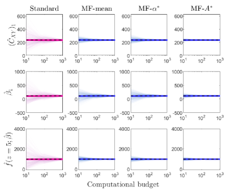
Figure 2: Analytical example: 500 realizations (semi-transparent colored lines) of estimators for first entry of $\hat{C}_{XY}$ (top row), first regression coefficient (middle row), and regression model prediction $\hat{f}(z=5;\hat{\beta})$, when true model statistics are known. Black dashed line denotes known true values and thick solid colored lines show the mean over realizations computed from different training data.

Experiments using inexact model statistics. Figures 3(b) and 3(c) plot the trace of the covariance for the 500 realizations of the standard and multifidelity regression estimators when the model statistics are estimated inexactly using pilot samples for each realization. Figure 3(b) uses a moderate pilot sample size of 100 whereas Figure 3(c) uses a small pilot sample size of 10. We find that using estimated model statistics to determine the sample allocation according to (10) yields a 1% (5%) variation in $m_{1}$ and a 5% (20%) variation in $m_{2}$ when 100 (10) pilot samples are used. Despite this variation in sample allocation, the multifidelity regression realizations have lower variance than the standard single-fidelity approach.

For this analytical example, the MF-$A^{*}$ strategy yields the greatest variance reduction even when it is computed from inexact model statistics, although the difference between its performance and that of the scalar coefficient choices becomes smaller as the model statistic estimate becomes poorer. The two choices of of scalar coefficient, MF-$\alpha^{*}$ and MF-mean, perform similarly when inexact model statistics are used in their calculation: the theoretically optimal MF-$\alpha^{*}$ barely outperforms the sub-optimal MF-mean strategy when 100 pilot samples are used, and sometimes underperforms when just 10 pilot samples are available. The good performance of the simpler MF-mean strategy in practical settings where model statistics must be estimated leads us to recommend it over the theoretically more optimal options that require estimations of more complex statistics.

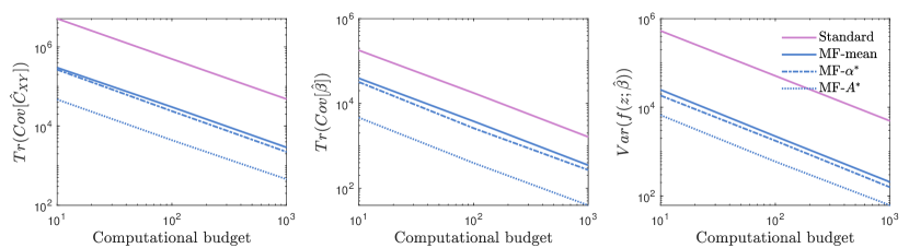
(a) True model statistics

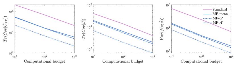
(b) 100 pilot samples

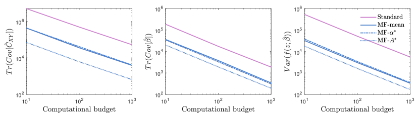
(c) 10 pilot samples

Figure 3: Comparing the effect of optimal control variate coefficients with respect to the minimization of the (generalized) variance of the estimators as described in Theorems 3.4 and 3.8 when (a) true model statistics are used compared to when model statistics are estimated from (b) 100 pilot samples and (c) 10 pilot samples for the three options proposed in Section 3.2.1 for the analytic example.

4.2 A PDE model problem

We now demonstrate our multifidelity linear regression method on a two-dimensional hydrogen combustion model with five parameters. The high- and low-fidelity models were originally developed in [5] and then used for sensitivity analysis in [56]. We follow the setup in [56], which we summarize in Section 4.2.1. Section 4.2.2 then presents results for this problem.

4.2.1 Convection-diffusion-reaction (CDR) problem

We consider a convection-diffusion-reaction model on a two-dimensional rectangular domain. The model assumes a premixed hydrogen flame at constant, uniform pressure, with constant, divergence-free velocity field, and equal, uniform molecular diffusivities for all species and temperatures. The dynamics of the system are described by a convection-diffusion-reaction equation with source terms modeled as in [12] as follows:

$$\begin{split}\frac{\partial u}{\partial t}&=\kappa\Delta u-U\nabla u+s(u,z)\\ s_{i}(u,z)&=\nu_{i}\left(\frac{W_{i}}{\rho_{\text{mix}}}\right)\left(\frac{\rho_{\text{mix}}Y_{F}}{W_{F}}\right)^{\nu_{F}}\left(\frac{\rho_{\text{mix}}Y_{O}}{W_{O}}\right)^{\nu_{O}}A_{\text{pe}}\exp\left(-\frac{E}{RT}\right),\,\quad\text{for }i=F,O,P,\\ s_{T}(u,z)&=s_{P}(u,z)Q.\end{split}$$ (27)

In (27), the thermo-chemical state is $u(z,t)=[Y_{F},Y_{O},Y_{P},T]^{\top}$, where $Y_{F}$, $Y_{O}$, and $Y_{P}$ are the mass fractions of the fuel, oxidizer, and product, respectively, and $T$ is the temperature; $\kappa$ is the molecular diffusivity, $U$ is the velocity field, and $s$ is the nonlinear reaction source term. The reaction modeled is a one-step hydrogen combustion given by $2\text{H}_{2}+\text{O}_{2}\rightarrow 2\text{H}_{2}\text{O}$, where hydrogen is the fuel, oxygen acts as the oxidizer, and water is the product. The source terms are defined using $A_{\text{pe}}$ as the pre-exponential factor of the Arrhenius equation, $E$ as the activation energy, $W_{i}$ as the molecular weight of species $i$, $\rho_{\text{mix}}$ as the density of the mixture, $R$ as the universal gas constant, and $Q$ as the heat of the reaction.

For our regression problem, the quantity of interest is the maximum temperature in the chamber at steady state. The input parameter vector for regression is given by

$$s=[A_{\text{pe}},E,T_{i},T_{0},\phi]\in[5.5\times 10^{11},1.5\times 10^{12}]\times[1.5\times 10^{3},9.5\times 10^{3}]\times[200,400]\times[850,1000]\times[0.5,1.5],$$

where $T_{i}$ is the temperature at the inlet, $T_{0}$ is the temperature of the left wall of the domain, and $\phi$ is the fuel:oxidizer ratio of the premixed inflow. The parameters $A_{\text{pe}}$ and $E$ are assumed to be log-uniformly distributed and $T_{i}$, $T_{0}$, and $\phi$ are assumed to be uniformly distributed. We fit a quadratic model to these five inputs, so that the feature vector $x$ has length 21 (one constant, five linear, and 15 quadratic features).

The high-fidelity data arises from a finite-difference solver that discretizes the spatial domain into a $73\times 37$ grid, resulting in $73\times 37\times 4=10804$ degrees of freedom that includes the mass fractions of each of the three chemical species as well as the temperature at each grid point. The low-fidelity data arises from a POD-DEIM projection-based reduced model [9] with 19 POD basis functions and 1 DEIM basis function (see [5] for details of the model reduction approach applied to this reacting flow problem). Statistics for these two models computed using a data set consisting of $2.4\times 10^{5}$ samples are presented in Table 2 [56]. This data set can be downloaded from https://github.com/elizqian/mfgsa. For all numerical experiments below, the covariance $C_{XX}$ is computed from all $2.4\times 10^{5}$ samples. The standard and multifidelity regression estimators for $\hat{C}_{XY}$ are computed by bootstrapping samples from this data set within budget constraints, assuming that high-fidelity data have cost $w_{1}=1.94$ and low-fidelity data have cost $w_{2}=6.2\text{e-}3$ as stated in [56].

model		$\mu_{i}$	$\sigma_{i}$	$\rho_{1i}$	$w_{i}$
High-fidelity (FD)	$f^{(1)}$	1406	276.1	1	1.94
Low-fidelity (POD-DEIM)	$f^{(2)}$	1349	356	0.95	6.2e-3

Table 2: High-sample model statistics for the high- and low-fidelity models for the CDR problem using $2.4\times 10^{5}$ samples [56].

4.2.2 Results: CDR problem

Results using high-sample model statistics estimates. Because analytical model statistics are not easily obtainable for this example, we first provide multifidelity regression results that use model statistics estimated from $10^{5}$ samples. For computational budgets of 10, 100, and 1000, these estimated model statistics yield the sample allocations tabulated in Table 3. Figure 4 then plots 500 realizations of the estimators for the first element of $\hat{C}_{XY}$, the first regression coefficient $\hat{\beta}_{1}$, and the learned model prediction at $z=a$ where $a$ is a given point in the input domain. The realizations are again plotted with some transparency; the mean of the estimator realizations is again shown in the solid colored line; and the estimators resulting from using $10^{5}$ high-fidelity samples is plotted using a dashed black line for reference. Figure 4 illustrates our theoretical results from Section 3: that the multifidelity estimators are unbiased (Theorem 3.1), and that when good estimates of the model statistics are known, the MF-$A^{*}$ optimal matrix coefficient $A^{*}$ yields greater variance reduction than the MF-$\alpha^{*}$ optimal scalar coefficient $\alpha^{*}$, which in turn yields greater variance reduction than the sub-optimal MF-mean $\alpha$.

Computational budget	$m_{1}$	$m_{2}$
10	4	250
100	43	2505
1000	435	24998

Table 3: Sample allocation based on (10) for the CDR problem when high-sample estimates of model statistics are available.

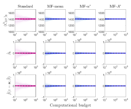
Figure 4: Illustrating unbiasedness of standard linear regression and multifidelity linear regression fits over 500 repetitions of training data for estimation of first entry of $\hat{C}_{XY}$ and regression coefficient along with the prediction $\hat{f}(z=a;\hat{\beta})$ where $a=[5.5\times 10^{11},6000,300,925,1]$ when high-sample estimates of model statistics are used for the CDR problem. Black dashed line denotes known true values and colored lines denote the estimates from 500 repetitions of training data.

Results using low-sample model statistic estimates. In Figure 5, we study the effect of using smaller pilot sample sizes to estimate the model statistics used to determine control variate coefficients and sample allocation. Figure 5(a) plots the (generalized) variance of $\hat{C}_{XY}$, $\hat{\beta}$, and $\hat{f}(z;\hat{\beta})$ when $10^{5}$ pilot samples are used, for reference. The generalized variance of the estimators is computed from 500 realizations of the standard/multifidelity linear regression estimators. Figure 5(b) shows the variance of the estimators when 100 pilot samples are used, and Figure 5(c) the results for just 10 pilot samples. We find that using estimated model statistics to determine the sample allocation according to (10) yields a 1% (10%) variation in $m_{1}$ and a 6% (25%) variation in $m_{2}$ when 100 (10) pilot samples are used. Despite this variation in sample allocation, the multifidelity regression realizations have lower variance than the standard single-fidelity approach.

For this PDE model problem, the gains from using MF-$A^{*}$ are not as significant as for the analytic example. In fact, for the smallest pilot sample size of 10 (Figure 5(c)), we see that MF-$A^{*}$ performs significantly worse than the scalar control variate coefficients. This is because the optimal $A^{*}$ choice depends on accurate estimation of the covariances $C_{12}$ and $C_{22}$ which are in $\mathbb{R}^{21\times 21}$ for this problem, and are thus difficult to estimate. This indicates that for complex engineering problems, the theoretically optimal MF-$A^{*}$ strategy should not be used when statistics must be estimated using limited pilot samples. However, multifidelity regressions using both choices of scalar coefficient perform well across different pilot sample sizes, yielding significant variance reduction when compared to standard linear regression for varying computational budgets. The optimal $\alpha^{*}$ performs better than the optimal $A^{*}$ because the choice of $\alpha^{*}$ relies only on accurate estimation of $\mathsf{Tr}(C_{12})$ and $\mathsf{Tr}(C_{22})$, which are scalar quantities which are easier to estimate from limited data. For this case, both scalar $\alpha$ multifidelity learned models trained with the lowest computational budget (just 4 high-fidelity samples) achieve a similar average error to standard learned models trained with $\mathcal{O}(100)$ high-fidelity samples, again demonstrating the efficacy of the multifidelity approach for learning robust and accurate models in the scarce data regime.

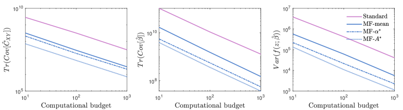
(a) High-sample model statistics using $10^{5}$ samples

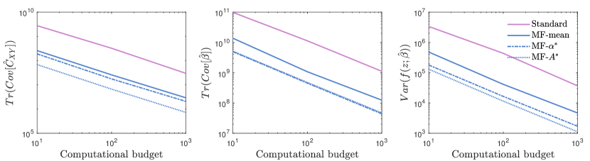
(b) 100 pilot samples

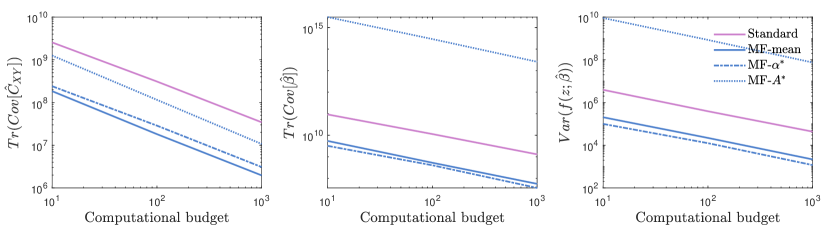
(c) 10 pilot samples

Figure 5: Comparing the effect of optimal control variate coefficients with respect to the minimization of trace of the covariance of the estimators as described in Theorems 3.4 and 3.8 when model statistics are (a) high-sample estimates using $10^{5}$ samples compared to model statistics estimated from (b) 100 pilot samples and (c) 10 pilot samples for the three options proposed in Section 3.2.1 for the CDR problem.

5 Conclusions and future work

We have introduced a multifidelity training strategy for linear regression problems which leverages data of varying fidelity and cost to improve the robustness of training to scarce high-fidelity data due to limited training budgets. Our approach is based on new multifidelity Monte Carlo estimators for the unknown linear regression coefficients, which we showed are unbiased with respect to the high-fidelity data distribution. We discussed multiple strategies for choosing the amount of data for each fidelity level, and for choosing the control variate coefficients in the multifidelity estimators, which can be viewed as hyperparameters of the method. We provide theoretical analyses showing that there are optimal choices of control variate coefficients when model statistics are known, and provide practical recommendations for choosing the hyperparameters when model statistics are unknown. Numerical experiments illustrate and verify our theoretical results and also demonstrate that the multifidelity training approach learns more robust linear regression models than a standard high-fidelity training approach when the training budget is limited and only scarce high-fidelity data are available.

Many directions exist for future work. To make this multifidelity training approach more generally applicable in scientific machine learning, new approaches must be developed for linear regression models with vector outputs as well as for nonlinear regression models. These new methods will be critical for learning surrogate models that describe dynamics of time-dependent engineering systems rather than the input-to-scalar-output map we have focused on in this work. Even within the linear regression framework that we have introduced here, several avenues for further theoretical and practical investigation remain, including analysis of the method to determine optimal budget allocations tailored to the linear regression problem (instead of using the heuristic based on mean estimation that we recommend here), and exploring hybrid or active data acquisition strategies where some data are given but more can be obtained within budget constraints.

Acknowledgments. The authors are grateful to Florian Schäfer and Rob Webber for helpful discussions. EQ acknowledges support from the US Department of Energy, Office of Advanced Scientific Computing Research (ASCR), Applied Mathematics Program, award DE-SC0024721. AC acknowledges support from the US Department of Energy (DOE) grant number DE-SC0021239.

References

- [1] Shady E Ahmed and Panos Stinis. A multifidelity deep operator network approach to closure for multiscale systems. Computer Methods in Applied Mechanics and Engineering, 414:116161, 2023.
- [2] Terrence Alsup and Benjamin Peherstorfer. Context-aware surrogate modeling for balancing approximation and sampling costs in multifidelity importance sampling and Bayesian inverse problems. SIAM/ASA Journal on Uncertainty Quantification, 11(1):285–319, 2023.
- [3] Kaushik Bhattacharya, Bamdad Hosseini, Nikola B Kovachki, and Andrew M Stuart. Model reduction and neural networks for parametric PDEs. The SMAI Journal of Computational Mathematics, 7:121–157, 2021.
- [4] Loïc Brevault, Mathieu Balesdent, and Ali Hebbal. Overview of gaussian process based multi-fidelity techniques with variable relationship between fidelities, application to aerospace systems. Aerospace Science and Technology, 107:106339, 2020.
- [5] M. Buffoni and K. Willcox. Projection-based model reduction for reacting flows. In 40th Fluid Dynamics Conference and Exhibit, page 5008, 2010.
- [6] Giuseppe Cataldo, Elizabeth Qian, and Jeremy Auclair. Multifidelity uncertainty quantification and model validation of large-scale multidisciplinary systems. Journal of Astronomical Telescopes, Instruments, and Systems, 8(3):038001, 2022.
- [7] Neil K Chada, Ajay Jasra, Kody JH Law, and Sumeetpal S Singh. Multilevel Bayesian deep neural networks. arXiv preprint arXiv:2203.12961, 2022.
- [8] Kwan J Chang, Raphael T Haftka, Gary L Giles, and Pi-Jen Kao. Sensitivity-based scaling for approximating structural response. Journal of Aircraft, 30(2):283–288, 1993.
- [9] S. Chaturantabut and D. Sorensen. Nonlinear model reduction via discrete empirical interpolation. SIAM Journal on Scientific Computing, 32(5):2737–2764, 2010.
- [10] Anirban Chaudhuri, John Jasa, Joaquim RRA Martins, and Karen E Willcox. Multifidelity optimization under uncertainty for a tailless aircraft. In 2018 AIAA Non-Deterministic Approaches Conference, page 1658, 2018.
- [11] Anirban Chaudhuri, Alexandre N Marques, and Karen Willcox. mfegra: Multifidelity efficient global reliability analysis through active learning for failure boundary location. Structural and Multidisciplinary Optimization, 64(2):797–811, 2021.
- [12] B. Cuenot and T. Poinsot. Asymptotic and numerical study of diffusion flames with variable lewis number and finite rate chemistry. Combustion and Flame, 104(1-2):111–137, 1996.
- [13] Subhayan De, Jolene Britton, Matthew Reynolds, Ryan Skinner, Kenneth Jansen, and Alireza Doostan. On transfer learning of neural networks using bi-fidelity data for uncertainty propagation. International Journal for Uncertainty Quantification, 10(6), 2020.
- [14] Subhayan De and Alireza Doostan. Neural network training using -regularization and bi-fidelity data. Journal of Computational Physics, 458:111010, 2022.
- [15] Subhayan De, Matthew Reynolds, Malik Hassanaly, Ryan N King, and Alireza Doostan. Bi-fidelity modeling of uncertain and partially unknown systems using DeepONets. arXiv preprint arXiv:2204.00997, 2022.
- [16] Maarten de Hoop, Daniel Zhengyu Huang, Elizabeth Qian, and Andrew Stuart. The cost-accuracy trade-off in operator learning with neural networks. Journal of Machine Learning, 1(3):299–341, 2022.
- [17] Nicola Demo, Marco Tezzele, and Gianluigi Rozza. A DeepONet multi-fidelity approach for residual learning in reduced order modeling. arXiv preprint arXiv:2302.12682, 2023.
- [18] Ionuț-Gabriel Farcaș, Benjamin Peherstorfer, Tobias Neckel, Frank Jenko, and Hans-Joachim Bungartz. Context-aware learning of hierarchies of low-fidelity models for multi-fidelity uncertainty quantification. Computer Methods in Applied Mechanics and Engineering, 406:115908, 2023.
- [19] M Giselle Fernández-Godino, Sylvain Dubreuil, Nathalie Bartoli, Christian Gogu, Sivaramakrishnan Balachandar, and Raphael T Haftka. Linear regression-based multifidelity surrogate for disturbance amplification in multiphase explosion. Structural and Multidisciplinary Optimization, 60:2205–2220, 2019.
- [20] Masahiro Fujisawa and Issei Sato. Multilevel Monte Carlo variational inference. The Journal of Machine Learning Research, 22(1):12741–12784, 2021.
- [21] Thomas Gerstner, Bastian Harrach, Daniel Roth, and Martin Simon. Multilevel Monte Carlo learning. arXiv preprint arXiv:2102.08734, 2021.
- [22] Michael B Giles. Multilevel Monte Carlo path simulation. Operations research, 56(3):607–617, 2008.
- [23] Michael B Giles. Multilevel Monte Carlo methods. Acta numerica, 24:259–328, 2015.
- [24] Mengwu Guo, Andrea Manzoni, Maurice Amendt, Paolo Conti, and Jan S Hesthaven. Multi-fidelity regression using artificial neural networks: Efficient approximation of parameter-dependent output quantities. Computer methods in applied mechanics and engineering, 389:114378, 2022.
- [25] Raphael T Haftka. Combining global and local approximations. AIAA journal, 29(9):1523–1525, 1991.
- [26] Jan S Hesthaven and Stefano Ubbiali. Non-intrusive reduced order modeling of nonlinear problems using neural networks. Journal of Computational Physics, 363:55–78, 2018.
- [27] Roger A Horn and Charles R Johnson. Matrix analysis. Cambridge university press, 2012.
- [28] Kurt Hornik, Maxwell Stinchcombe, and Halbert White. Multilayer feedforward networks are universal approximators. Neural networks, 2(5):359–366, 1989.
- [29] Amanda A Howard, Mauro Perego, George E Karniadakis, and Panos Stinis. Multifidelity deep operator networks. arXiv preprint arXiv:2204.09157, 2022.
- [30] Jaeyub Hyun, Anirban Chaudhuri, Karen E Willcox, and Hyunsun A Kim. Multifidelity robust topology optimization for material uncertainties with digital manufacturing. In AIAA SCITECH 2023 Forum, page 2038, 2023.
- [31] Su Jiang and Louis J Durlofsky. Use of multifidelity training data and transfer learning for efficient construction of subsurface flow surrogate models. Journal of Computational Physics, 474:111800, 2023.
- [32] Marc C Kennedy and Anthony O’Hagan. Predicting the output from a complex computer code when fast approximations are available. Biometrika, 87(1):1–13, 2000.
- [33] Duane L Knill, Anthony A Giunta, Chuck A Baker, Bernard Grossman, William H Mason, Raphael T Haftka, and Layne T Watson. Response surface models combining linear and euler aerodynamics for supersonic transport design. Journal of Aircraft, 36(1):75–86, 1999.
- [34] Loic Le Gratiet and Josselin Garnier. Recursive co-kriging model for design of computer experiments with multiple levels of fidelity. International Journal for Uncertainty Quantification, 4(5), 2014.
- [35] Zongyi Li, Nikola Kovachki, Kamyar Azizzadenesheli, Burigede Liu, Kaushik Bhattacharya, Andrew Stuart, and Anima Anandkumar. Fourier neural operator for parametric partial differential equations. ICLR 2021; arXiv:2010.08895, 2020.
- [36] Dehao Liu and Yan Wang. Multi-fidelity physics-constrained neural network and its application in materials modeling. Journal of Mechanical Design, 141(12):121403, 2019.
- [37] Lu Lu, Pengzhan Jin, Guofei Pang, Zhongqiang Zhang, and George Em Karniadakis. Learning nonlinear operators via DeepONet based on the universal approximation theorem of operators. Nature Machine Intelligence, 3(3):218–229, 2021.
- [38] Lu Lu, Raphaël Pestourie, Steven G Johnson, and Giuseppe Romano. Multifidelity deep neural operators for efficient learning of partial differential equations with application to fast inverse design of nanoscale heat transport. Physical Review Research, 4(2):023210, 2022.
- [39] Dingcheng Luo, Thomas O’Leary-Roseberry, Peng Chen, and Omar Ghattas. Efficient PDE-constrained optimization under high-dimensional uncertainty using derivative-informed neural operators. arXiv preprint arXiv:2305.20053, 2023.
- [40] Alexandre Marques, Remi Lam, and Karen Willcox. Contour location via entropy reduction leveraging multiple information sources. Advances in neural information processing systems, 31, 2018.
- [41] Mohamed Mehana, Aleksandra Pachalieva, Ashish Kumar, Javier Santos, Daniel O’Malley, William Carey, Mukul Sharma, and Hari Viswanathan. Prediction and uncertainty quantification of shale well performance using multifidelity Monte Carlo. Gas Science and Engineering, 110:204877, 2023.
- [42] Xuhui Meng and George Em Karniadakis. A composite neural network that learns from multi-fidelity data: Application to function approximation and inverse PDE problems. Journal of Computational Physics, 401:109020, 2020.
- [43] I. Mezić. Analysis of fluid flows via spectral properties of the Koopman operator. Annual Review of Fluid Mechanics, 45:357–378, 2013.
- [44] Igor Mezić. Spectral properties of dynamical systems, model reduction and decompositions. Nonlinear Dynamics, 41(1):309–325, 2005.
- [45] Christian Moya and Guang Lin. Bayesian, multifidelity operator learning for complex engineering systems–a position paper. Journal of Computing and Information Science in Engineering, 23(6), 2023.
- [46] Nicholas H Nelsen and Andrew M Stuart. The random feature model for input-output maps between banach spaces. SIAM Journal on Scientific Computing, 43(5):A3212–A3243, 2021.
- [47] Leo WT Ng and Karen E Willcox. Multifidelity approaches for optimization under uncertainty. International Journal for numerical methods in Engineering, 100(10):746–772, 2014.
- [48] Thomas O’Leary-Roseberry, Peng Chen, Umberto Villa, and Omar Ghattas. Derivative informed neural operator: An efficient framework for high-dimensional parametric derivative learning. arXiv preprint arXiv:2206.10745, 2022.
- [49] Lucia Parussini, Daniele Venturi, Paris Perdikaris, and George E Karniadakis. Multi-fidelity gaussian process regression for prediction of random fields. Journal of Computational Physics, 336:36–50, 2017.
- [50] B. Peherstorfer, K. Willcox, and M. Gunzburger. Optimal model management for multifidelity Monte Carlo estimation. SIAM Journal on Scientific Computing, 38(5):A3163–A3194, 2016.
- [51] Benjamin Peherstorfer and Karen Willcox. Data-driven operator inference for nonintrusive projection-based model reduction. Computer Methods in Applied Mechanics and Engineering, 306:196–215, 2016.
- [52] Paris Perdikaris, Maziar Raissi, Andreas Damianou, Neil D Lawrence, and George Em Karniadakis. Nonlinear information fusion algorithms for data-efficient multi-fidelity modelling. Proceedings of the Royal Society A: Mathematical, Physical and Engineering Sciences, 473(2198):20160751, 2017.
- [53] Matthias Poloczek, Jialei Wang, and Peter Frazier. Multi-information source optimization. Advances in neural information processing systems, 30, 2017.
- [54] Elizabeth Qian, Ionut-Gabriel Farcas, and Karen Willcox. Reduced operator inference for nonlinear partial differential equations. SIAM Journal on Scientific Computing, 44(4), 2022.
- [55] Elizabeth Qian, Boris Kramer, Benjamin Peherstorfer, and Karen Willcox. Lift & Learn: Physics-informed machine learning for large-scale nonlinear dynamical systems. Physica D: Nonlinear Phenomena, Volume 406, 2020.
- [56] Elizabeth Qian, Benjamin Peherstorfer, Daniel O’Malley, Velimir V Vesselinov, and Karen Willcox. Multifidelity Monte Carlo estimation of variance and sensitivity indices. SIAM/ASA Journal on Uncertainty Quantification, 6(2):683–706, 2018.
- [57] Milad Ramezankhani, Amir Nazemi, Apurva Narayan, Heinz Voggenreiter, Mehrtash Harandi, Rudolf Seethaler, and Abbas S Milani. A data-driven multi-fidelity physics-informed learning framework for smart manufacturing: a composites processing case study. In 2022 IEEE 5th International Conference on Industrial Cyber-Physical Systems (ICPS), pages 01–07. IEEE, 2022.
- [58] Reuven Y Rubinstein and Ruth Marcus. Efficiency of multivariate control variates in monte carlo simulation. Operations Research, 33(3):661–677, 1985.
- [59] Vignesh Sella, Julie Pham, Anirban Chaudhuri, and Karen E Willcox. Projection-based multifidelity linear regression for data-poor applications. In AIAA SCITECH 2023 Forum, page 0916, 2023.
- [60] Maolin Shi, Liye Lv, Wei Sun, and Xueguan Song. A multi-fidelity surrogate model based on support vector regression. Structural and Multidisciplinary Optimization, 61:2363–2375, 2020.
- [61] Yuyang Shi and Rob Cornish. On multilevel Monte Carlo unbiased gradient estimation for deep latent variable models. In International Conference on Artificial Intelligence and Statistics, pages 3925–3933. PMLR, 2021.
- [62] Dong H Song and Daniel M Tartakovsky. Transfer learning on multifidelity data. Journal of Machine Learning for Modeling and Computing, 3(1), 2022.
- [63] R. Swischuk, L. Mainini, B. Peherstorfer, and K. Willcox. Projection-based model reduction: Formulations for physics-based machine learning. Computers and Fluids, 179:704–717, 2019.
- [64] Aretha L Teckentrup, Robert Scheichl, Michael B Giles, and Elisabeth Ullmann. Further analysis of multilevel monte carlo methods for elliptic PDEs with random coefficients. Numerische Mathematik, 125:569–600, 2013.
- [65] Matthew O Williams, Ioannis G Kevrekidis, and Clarence W Rowley. A data–driven approximation of the Koopman operator: Extending dynamic mode decomposition. Journal of Nonlinear Science, 25:1307–1346, 2015.
- [66] Matthew O Williams, Clarence Worth Rowley, and Yannis Kevrekidis. A kernel-based method for data-driven Koopman spectral analysis. Journal of Computational Dynamics, 2(2):247–265, 2015.
- [67] Yiming Zhang, Nam H. Kim, Chanyoung Park, and Raphael T. Haftka. Multifidelity surrogate based on single linear regression. AIAA Journal, 56(12):4944–4952, 2018.