Environment-Induced Information Scrambling Transition with Charge Conservations

Abstract

In generic closed quantum systems, the complexity of operators increases under time evolution governed by the Heisenberg equation, reflecting the scrambling of local quantum information. However, when systems interact with an external environment, the system-environment coupling allows operators to escape from the system, inducing a dynamical transition between the scrambling phase and the dissipative phase. This transition is known as the environment-induced information scrambling transition, originally proposed in Majorana fermion systems. In this work, we advance this dicovery by investigating the transition in charge-conserved systems with space-time randomness. We construct solvable Brownian Sachdev-Ye-Kitaev models of complex fermions coupled to an environment, enabling the analytical computation of operator growth. We determine the critical dissipation strength, which is proportional to $n(1-n)$ with $n$ being the density of the complex fermions, arising from the suppression in the quantum Lyapunov exponent due to the Pauli blockade in the scattering process. We further analyze the density dependence of maximally scrambled operators at late time. Our results shed light on the intriguing interplay between information scrambling, dissipation, and conservation laws.

I Introduction

Recent years have witnessed breakthroughs in understanding the dynamics of quantum information in many-body systems. In particular, there has been considerable attention focusing on information scrambling Hayden and Preskill (2007); Sekino and Susskind (2008); Shenker and Stanford (2015); Roberts et al. (2015); Islam et al. (2015); Li et al. (2017); Gärttner et al. (2017); Brydges et al. (2019); Sánchez et al. (2019); Landsman et al. (2019); Joshi et al. (2020); Blok et al. (2021); Domínguez et al. (2021); Domínguez and Álvarez (2021); Mi et al. (2021); Cotler et al. (2022); Sánchez et al. (2022), which describes how local information disperses throughout the entire system. As an illustration, suppose we initially encode a single-qubit state $|\psi\rangle$ locally in a many-body wavefunction by preparing a product state $|\Psi\rangle=|\psi\rangle\otimes|0\rangle\otimes...\otimes|0\rangle$. We then proceed to evolve the entire system in time, described by an evolution operator $\hat{U}$. Consequently, the state of the system becomes $|\Psi(t)\rangle=\hat{U}~{}|\Psi\rangle$. In general, this evolution will build up entanglement between different qubits in the many-body system, causing the encoded information to become extended. To read off the encoded information by only observing operators $\{\hat{O}^{m}_{1}\}$ acting locally on the first qubit, one should apply to $|\Psi(t)\rangle$ the backwardly evolved operators $\{\hat{O}_{1}^{m}(-t)\equiv\hat{U}\hat{O}^{m}_{1}\hat{U}^{\dagger}\}$, which is highly complex and non-local. A quantitative measure of operator complexity is provided by the operator size distribution, extensively investigated in solvable models or through numerical simulations Roberts et al. (2015); Nahum et al. (2018); Qi and Streicher (2019); von Keyserlingk et al. (2018); Khemani et al. (2018a); Hunter-Jones (2018); Chen and Lucas (2021); Lucas (2019); Chen et al. (2020a); Lucas and Osborne (2020); Yin and Lucas (2021); Zhou and Swingle (2021); Dias et al. (2021); Wu et al. (2021); Gu et al. (2022); Zhang and Gu (2023); Liu and Zhang (2024); Gao et al. (2023, 2024). For systems with all-to-all interactions, the operator size exhibits exponential growth in the early-time regime and eventually ”thermalizes” to a maximally scrambled operator modeled by a uniform distribution among all operators.

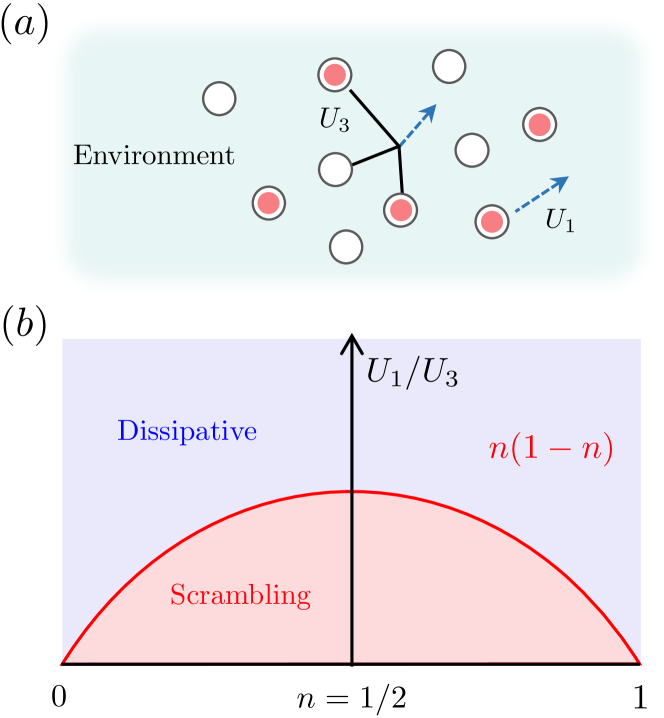
Figure 1: (a) Schematics of the all-to-all interacting systems with charge conservation. Here, each red dot corresponds to a charge occupation. $U_{3}$ corresponds to an interaction between three system fermions and a single environment fermion, and $U_{1}$ represents the hopping between the system and environment. (b) The phase diagram of the model, in which the information scrambling transition occurs at $U_{1}/U_{3}=n(1-n)$.

Later, the study of information scrambling has been extended to systems that are embedded in environments Zhang and Yu (2023); Bhattacharya et al. (2022); Liu et al. (2022); Schuster and Yao (2022); Weinstein et al. (2022). In the presence of system-environment couplings, an operator may disappear from the system and disperses into the environment. This process can be viewed as a dissipation in the operator space. Refs. Zhang and Yu (2023); Weinstein et al. (2022) propose that actually an environment-induced information scrambling transition can occur when the system-environment couplings are fine tuned; this transition separates a scrambling phase and a dissipative phase. In the scrambling phase, the operator size within the system continues to increase to an order of $N$ (where $N$ is the system size), as in closed systems. Conversely, in the dissipative phase, the size decreases exponentially over time. Additionally, it is noted that the distribution of operator sizes displays a power-law decay at the critical point. Explicit examples include random circuit models Weinstein et al. (2022) and Brownian SYK models Kitaev (2015); Maldacena and Stanford (2016); Kitaev and Suh (2018); Saad et al. (2018); Sünderhauf et al. (2019) with Majorana fermions Zhang and Yu (2023). Both models feature space-time randomness and lacking any discernible global symmetry.

However, it is well-established that conservation laws exert profound implications on the dynamics of quantum many-body systems. For instance, in systems with charge conservation, the out-of-time-order correlator Shenker and Stanford (2015); Roberts et al. (2015); Larkin and Ovchinnikov (1969); Kitaev (2014) in random circuits exhibits power-law tails attributed to the diffusion of local charges Rakovszky et al. (2018); Khemani et al. (2018b). It is also known that the Rényi entropies (with Rényi index $\alpha>1$) of a half-infinite system grow as $\leq\sqrt{t\ln t}$ Huang (2019); Rakovszky et al. (2019) after a quantum quench. In systems at low/high densities $n$, both the quantum Lyapunov exponent and the butterfly velocity are suppressed by a polynomial of $n$ due to the Pauli blockade of the effective Hilbert space Chen et al. (2020b); Zhang (2023); Agarwal and Xu (2020). Therefore, it is interesting to explore the the fate of the environment-induced information scrambling transition in systems with charge conservations.

In this work, we construct a solvable complex Brownian SYK model embedded in an environment, as illustrated in FIG. 1 (a). The total system exhibits a weak U(1) symmetry, allowing for the interchange of charges between the system and the environment. By analyzing generic system-environment couplings, we identify dominant terms in the low/high-density limit. The main contribution to the information scrambling in the system comes from a four-body interaction, yielding a quantum Lyapunov exponent $\varkappa_{\text{eff}}\propto n(1-n)U_{3}$, where $U_{3}$ is the interaction strength. For comparison, dissipation is governed by a direct hopping between the system and the environment, with an effective dissipation rate $U_{1}$ independent of the density $n$. Consequently, we expect that the information scrambling transition shall occur at $U_{1}/U_{3}\propto n(1-n)$, as sketched in FIG. 1 (b). This expectation agrees with an analytically calculation using the complex Brownian SYK model. We further analyze the late-time regime using the scramblon effective theory Gu et al. (2022); Stanford et al. (2022), which unveils the renormalization of maximally scrambled operator.

II Model and Two-point functions

We consider a Brownian SYK model of $N$ complex fermions $\hat{c}_{j}$. The Hamiltonian of the system reads

$$\hat{H}_{S}=\sum_{q}\sum_{i_{1}<...<i_{\frac{q}{2}}}\sum_{j_{1}<...<j_{\frac{q}{2}}}J_{\{i_{l},j_{l}\}}(t)\hat{c}^{\dagger}_{i_{1}}\hat{c}^{\dagger}_{i_{2}}...\hat{c}^{\dagger}_{i_{\frac{q}{2}}}\hat{c}_{j_{1}}\hat{c}_{j_{2}}...\hat{c}_{j_{\frac{q}{2}}},$$ (1)

where the coupling strengthes $J_{\{i_{l},j_{l}\}}(t)$ are independent Brownian variables with zero expectation and

$$\overline{J_{\{i_{l},j_{l}\}}(t)J_{\{i_{l},j_{l}\}}(t^{\prime})^{*}}=\frac{J_{q}\delta(t-t^{\prime})}{\frac{q}{2}!(\frac{q}{2}-1)!N^{q-1}}.$$ (2)

Here, the normalization factor is chosen to cancel the symmetry factor of self-energies. We then couple the system to a microscopic environment, which contains complex fermions $\hat{e}_{a}$ with $a\in\{1,2,...,M\}$ Chen et al. (2017); Zhang (2019); Almheiri et al. (2019). We assume $M\gg N$ to ensure that the environment contains much more degrees of freedoms. We consider a generic coupling Hamiltonian between the system and the environment

$$\hat{H}_{SE}={\sum_{\{p_{l}\}}}^{\prime}\sum_{\{i_{l},j_{l},a_{k},b_{k}\}} U_{\{i_{l},j_{l},a_{k},b_{k}\}}(t)\hat{c}^{\dagger}_{i_{1}}...\hat{c}^{\dagger}_{i_{p_{1}}}\hat{c}_{j_{1}}...\hat{c}_{j_{p_{2}}}$$ (3)

$$\times\hat{e}^{\dagger}_{a_{1}}...\hat{e}^{\dagger}_{a_{p_{3}}}\hat{e}_{b_{1}}...\hat{e}_{b_{p_{4}}},$$

where we use $(p_{1},p_{2},p_{3},p_{4})$ to count the number of $(\hat{c}^{\dagger},\hat{c},\hat{e}^{\dagger},\hat{e})$ operators. We impose the conservation of the particle number $\hat{Q}=\sum_{i}\hat{c}^{\dagger}_{i}\hat{c}_{i}+\sum_{a}\hat{e}^{\dagger}_{a}\hat{e}_{a}$ by restricting the summation over $\{p_{l}\}$ to partitions satisfying $p_{1}+p_{3}=p_{2}+p_{4}$. The variance of the system-environment couplings are

$$\overline{U_{\{i_{l},j_{l},a_{k},b_{k}\}}(t)U_{\{i_{l},j_{l},a_{k},b_{k}\}}(t^{\prime})^{*}}=\frac{p_{2}U_{\{p_{l}\}}\delta(t-t^{\prime})}{\prod_{l=1}^{4}(p_{l}!)~{}N^{p_{1}+p_{2}-1}M^{p_{3}+p_{4}}}.$$ (4)

Since the time dependence of the coupling strengths breaks time translational invariance, the only tuning parameter for the steady state of the model is the charge density $n$. Employing a grand canonical ensemble, the steady-state density matrix is given by $\rho=\mathcal{Z}^{-1}e^{-\mu\hat{Q}}$, where $\mathcal{Z}=\text{tr}[e^{-\mu\hat{Q}}]$. The density $n$ can be related to the chemical potential $\mu$ by

$$n=\langle\hat{c}^{\dagger}_{i}\hat{c}_{i}\rangle=\langle\hat{e}^{\dagger}_{a}\hat{e}_{a}\rangle=\frac{1}{e^{\mu}+1}.$$ (5)

The steady-state properties can be analyzed using a Keldysh path-integral approach, which includes a forward evolution branch $u$ and a backward evolution branch $d$:

(6)

The two-point function on this contour is a two-by-two matrix $G^{ss^{\prime}}(t)=\langle c^{s}_{i}(t)\bar{c}^{s^{\prime}}_{i}(0)\rangle$, where $s,s^{\prime}\in\{u,d\}$ labels fields on different branches. In the large-$N$ limit, the self-energy only receives contributions from melon diagrams; the Schwinger-Dyson equation reads Zhang et al. (2020)

$$\begin{pmatrix}G^{uu}&G^{ud}\\ G^{du}&G^{dd}\end{pmatrix}=\begin{pmatrix}-i\omega-\Sigma^{uu}&-\Sigma^{ud}\\ -\Sigma^{du}&i\omega-\Sigma^{dd}\end{pmatrix}^{-1},$$ (7)

with self-energies

$$\Sigma^{uu}(\omega)=\Sigma^{dd}(\omega)=-\frac{\Gamma}{2}(1-2n),$$ (8)

$$\Sigma^{ud}(\omega)=-\Gamma n,\ \ \ \ \ \ \ \Sigma^{du}(\omega)=\Gamma(1-n),$$

where we have introduced the quasi-particle lifetime

$$\Gamma=\sum_{q}J_{q}[n(1-n)]^{\frac{q}{2}-1}+{\sum_{\{p_{l}\}}}^{\prime}U_{\{p_{l}\}}[n(1-n)]^{\frac{\sum_{l}p_{l}}{2}-1}.$$ (9)

Performing the inverse Fourier transform, we find Green’s functions in the time domain

$$G(t)=\begin{pmatrix}\frac{1}{2}-n+\frac{1}{2}\text{sgn}(t)&-n\\ 1-n&\frac{1}{2}-n-\frac{1}{2}\text{sgn}(t)\end{pmatrix}e^{-\frac{\Gamma|t|}{2}}.$$ (10)

This determines the retarded and advanced Green’s functions

$$G^{\text{R/A}}(t)=\mp i\theta(\pm t)~{}\text{tr}\left[\rho\{c_{i}(t),c_{i}^{\dagger}(0)\}\right]=\mp i\theta(\pm t)e^{-\frac{\Gamma|t|}{2}}.$$ (11)

III Operator size for complex fermions

We investigate the information scrambling in our model by computing the operator size growth. Our aim is to study operator growth in systems embedded in an environment at arbitrary density $n$. To motivate its general definition, we first consider the half-filling case $\mu=0$, for which the density matrix $\rho$ can be neglected. We introduce a orthonormal basis

$$\{\hat{O}_{j}^{m}\}=\{I,\hat{c}_{j}+\hat{c}_{j}^{\dagger},i(\hat{c}_{j}-\hat{c}_{j}^{\dagger}),2\hat{c}_{j}^{\dagger}\hat{c}_{j}-1\},$$ (12)

with $m\in\{1,2,3,4\}$ on each system fermion mode Zhang (2023). Here, the addition of $-1$ to the particle number operator ensures orthogonality with the identity. We assign a size to each local basis operator as $\{s_{m}\}=\{0,1,1,2\}$. This definition matches the standard convention Roberts et al. (2018) if we split each complex fermion into two Majorana fermions. A generic operator $\hat{O}(t)$ can be expanded as

$$\hat{O}(t)=\sum_{\{m_{i}\}}C_{m_{1}m_{2}...m_{N}}(t)\hat{O}_{1}^{m_{1}}\hat{O}_{2}^{m_{2}}...\hat{O}_{N}^{m_{N}}\otimes\hat{O}_{E},$$ (13)

where $\hat{O}_{E}$ is an operator supported solely within the environment. We assume $\hat{O}$ is some simple operator, such as $\hat{c}_{1}$. We define the size of each string operator $\hat{O}_{1}^{m_{1}}...\hat{O}_{N}^{m_{N}}\otimes\hat{O}_{E}$ as a summation $s_{\{m_{i}\}}=\sum_{i=1}^{N}s_{m_{i}}$. The operator size distribution $P_{0}(n,t)$ at half-filling $\mu=0$ then reads

$$P_{0}(s,t)=\sum_{\{m_{i}\}}\left|C_{m_{1}m_{2}...m_{N}}(t)\right|^{2}\delta_{s,s_{\{m_{i}\}}}\langle\hat{O}_{E}^{\dagger}\hat{O}_{E}\rangle.$$ (14)

Here, $\langle\hat{O}\rangle\equiv 2^{-M-N}\text{tr}[\hat{O}]$ measures the norm of the environment operator. For later convenience, we further introduce its generating function $Z_{0}(\nu,t)=\sum_{s}e^{-\nu s}P_{0}(s,t)$.

By generalizing analysis in closed systems Zhang (2023), we can express $Z(\mu,t)$ as a correlation function on the doubled Hilbert space by introducing an auxiliary copy of the total system, which includes system fermions $\hat{\xi}_{j}$ and environment fermions $\eta_{a}$. We pair up $(c_{j},\xi_{j})$ and $(e_{a},\eta_{a})$ by introducing a maximally entangled state

$$|I\rangle=\otimes_{j=1}^{N}\left[\frac{|01\rangle_{j}+|10\rangle_{j}}{\sqrt{2}}\right]\otimes_{a=1}^{M}\left[\frac{|01\rangle_{a}+|10\rangle_{a}}{\sqrt{2}}\right].$$ (15)

With the help of $|I\rangle$, we can map each operator $\hat{O}(t)$ into a state $|\hat{O}(t)\rangle=\hat{O}(t)|I\rangle$. We then look for a size operator $\hat{S}_{0}=\sum_{j=1}^{N}\hat{s}_{0,j}$, which satisfies

$$\hat{s}_{0,j}|\hat{O}^{m}_{j}\rangle=s_{m}|\hat{O}^{m}_{j}\rangle.$$ (16)

It is straightforward to check that we can choose

$$\hat{s}_{0,j}=\frac{1}{2}\left[(c_{j}^{\dagger}-\xi_{j}^{\dagger})(c_{j}-\xi_{j})+(c_{j}+\xi_{j})(c_{j}^{\dagger}+\xi_{j}^{\dagger})\right].$$ (17)

Therefore, the generating function can be expressed as

$$Z_{0}(\nu,t)=\langle\hat{O}(t)|e^{-\nu\hat{S}_{0}}|\hat{O}(t)\rangle.$$ (18)

Now, we consider adding a restriction to the Hilbert space to focus on the subspace with a general density $n$. The situation here closely parallels the definition of operator size at finite temperature Gu et al. (2022); Zhang and Gu (2023). In the grand canonical ensemble, the restriction can be incorporated by replacing $|\hat{O}(t)\rangle$ with

$$|\hat{O}(t)\rangle_{\mu}\equiv\frac{|\rho^{\frac{1}{4}}\hat{O}(t)\rho^{\frac{1}{4}}\rangle}{\sqrt{\langle\rho^{\frac{1}{4}}\hat{O}(t)\rho^{\frac{1}{4}}|\rho^{\frac{1}{4}}\hat{O}(t)\rho^{\frac{1}{4}}\rangle}}=\frac{|\rho^{\frac{1}{4}}\hat{O}(t)\rho^{\frac{1}{4}}\rangle}{\sqrt{\langle\hat{O}\rho^{\frac{1}{2}}\hat{O}\rho^{\frac{1}{2}}\rangle}}.$$ (19)

Then, we choose to modify the size operator $\hat{S}_{\mu}\equiv\sum_{j=1}^{N}\hat{s}_{\mu,j}$ correspondingly such that identity operator has no size $\hat{s}_{\mu,j}|I\rangle_{\mu}=0$. A convenient choice is Zhang (2023)

$$\hat{s}_{\mu,j}={A(\mu)}\Big{[} (e^{\frac{\mu}{4}}\hat{c}_{j}^{\dagger}-e^{-\frac{\mu}{4}}\hat{\xi}_{j}^{\dagger})(e^{\frac{\mu}{4}}\hat{c}_{j}-e^{-\frac{\mu}{4}}\hat{\xi}_{j})$$ (20)

$$+(e^{-\frac{\mu}{4}}\hat{c}_{j}+e^{\frac{\mu}{4}}\hat{\xi}_{j})(e^{-\frac{\mu}{4}}\hat{c}_{j}^{\dagger}+e^{\frac{\mu}{4}}\hat{\xi}_{j}^{\dagger})\Big{]}.$$

Here, $A(\mu)$ is an overall normalization factor that should satisfy $A(0)=1/2$. The size operator $\hat{s}_{\mu,j}$ is positive semi-definite and measures ”excitations” relative to the reference state $|I\rangle_{\mu}$. In this work, we fix $A(\mu)=({2\cosh(\mu/2)})^{-1}=\sqrt{n(1-n)}$ by further requiring

$$\hat{s}_{\mu,j}|\hat{c}_{j}\rangle_{\mu}=|\hat{c}_{j}\rangle_{\mu}.$$ (21)

Putting all ingredients together, we define the generating function at finite chemical potential as

$$Z_{\mu}(\nu,t)=~{}_{\mu}\langle\hat{O}(t)|e^{-\nu\hat{S}_{\mu}}|\hat{O}(t)\rangle_{\mu},$$ (22)

and the operator size distribution $P_{\mu}(s,t)$ is its inverse Laplace transform. By definition, we have $Z_{\mu}(0,t)=1$, which fixes the normalization $\sum_{s}P_{\mu}(s,t)=1$.

IV Evolution of Operator Size

The information scrambling in chaotic systems with all-to-all interactions can be divided into two regimes: the early-time regime with $t\sim O(1)$ and the late-time regime $t\sim\ln N$. In Ref. Zhang and Yu (2023), we demonstrate the existence of the environment-induced information scrambling transition in Majorana systems by computing the size distribution for single fermion operator in the early-time regime. In this section, we extend the calculation to our complex Brownian SYK models with $\hat{O}=\hat{c}_{1}$.

The study of $Z_{\mu}(\nu,t)$ requires introducing the doubled Keldysh contour Aleiner et al. (2016). As a warm-up, we first consider the average operator size $\overline{S}$, which reads

$$\overline{S}= ~{}_{\mu}\langle\hat{c}_{1}(t)|\hat{S}_{\mu}|\hat{c}_{1}(t)\rangle_{\mu}=\sum_{j}\langle\rho^{\frac{1}{2}}\{\hat{c}_{1}(t),\hat{c}_{j}\}\rho^{\frac{1}{2}}\{\hat{c}_{1}(t),\hat{c}_{j}\}\rangle$$ (23)

$$+\sum_{j}\langle\rho^{\frac{1}{2}}\{\hat{c}_{1}(t),\hat{c}_{j}^{\dagger}\}\rho^{\frac{1}{2}}\{\hat{c}_{1}(t),\hat{c}_{j}^{\dagger}\}\rangle,$$

where, we have used $\langle\hat{c}_{1}^{\dagger}\rho^{\frac{1}{2}}\hat{c}_{1}\rho^{\frac{1}{2}}\rangle=\sqrt{n(1-n)}$. In the path-integral approach, these four-point functions correspond to

(24)

In addition to the index $s\in\{u,d\}$, we further introduce a world index $w\in\{1,2\}$ that distinguishes the two forward/backward evolution branches. Here, black dots represent the insertion of $\hat{c}_{1}$ or $\hat{c}_{1}^{\dagger}$. Red dots represent the source term due to the size operator $\hat{S}_{\mu}$. In other words, we have

$$\overline{S}= \sum_{j}\left<T_{\mathcal{C}}\,c^{u,2}_{1}(t)\overline{c}^{u,1}_{1}(t)\left[c_{j}^{u,2}(0)-c_{j}^{d,2}(0)\right]\left[\bar{c}_{j}^{d,1}(0)-\bar{c}_{j}^{u,1}(0)\right]\right>$$ (25)

$$+\left<T_{\mathcal{C}}\,c^{u,2}_{1}(t)\overline{c}^{u,1}_{1}(t)\left[\bar{c}_{j}^{u,2}(0)-\bar{c}_{j}^{d,2}(0)\right]\left[c_{j}^{d,1}(0)-c_{j}^{u,1}(0)\right]\right>.$$

Here, the minus sign arises from the anti-commutation relation of Grassmann fields, and $T_{\mathcal{C}}$ denotes the contour ordering operator. Generalizing the discussion to the generating function $Z_{\mu}(\nu,t)$, we have

$$Z_{\mu}(\nu,t) =\frac{\left<T_{\mathcal{C}}\,c^{u,2}_{1}(t)\overline{c}^{u,1}_{1}(t)e^{-\Delta I}\right>}{\sqrt{n(1-n)}},$$ (26)

with souce term

$${\Delta I}=C(\nu,\mu) \sum_{j}\Bigg{(}\left[c_{j}^{u,2}(0)-c_{j}^{d,2}(0)\right]\left[\bar{c}_{j}^{d,1}(0)-\bar{c}_{j}^{u,1}(0)\right]$$ (27)

$$-\left[\bar{c}_{j}^{u,2}(0)-\bar{c}_{j}^{d,2}(0)\right]\left[c_{j}^{d,1}(0)-c_{j}^{u,1}(0)\right]\Bigg{)},$$

where $C(\nu,\mu)=(1-e^{-\nu})A(\mu)$ denotes the strength of the source term.

To derive the equation for $Z_{\mu}(\nu,t)$, we introduce the interworld Wightmann function

$$G^{W}(t_{1},t_{2})=\left<T_{\mathcal{C}}\,c^{u,2}(t_{1})\bar{c}^{u,1}(t_{2})e^{-\Delta I}\right>,$$ (28)

Using the symmetry when interchanging two worlds, this definition can be equivalently expressed as $G^{W}(t_{1},t_{2})=\left<T_{\mathcal{C}}\,\bar{c}^{u,2}(t_{2})c^{u,1}(t_{1})e^{-\Delta I}\right>$. The interworld Wightmann function satisfies the Schwinger-Dyson equation Zhang et al. (2020); Zhang and Yu (2023)

$$G^{W}(t_{1},t_{2})=\int dt_{3}dt_{4}~{}G^{R}(t_{1}-t_{3})\Sigma^{W}(t_{3},t_{4})G^{A}(t_{4}-t_{2}).$$ (29)

with self-energy

$$\Sigma^{W}(t,t^{\prime})= \delta(t-t^{\prime})\Bigg{(}\sum_{q}J_{q}G^{W}(t,t)^{q-1}-C(\nu,\mu)\delta(t)$$ (30)

$$+{\sum_{\{p_{l}\}}}^{\prime}U_{\{p_{l}\}}G^{W}(t,t)^{p_{1}+p_{2}-1}[n(1-n)]^{\frac{p_{3}+p_{4}}{2}}\Bigg{)}.$$

Finally, we set $t_{1}=t_{2}=t$ and apply the operator $(\partial_{t}+\Gamma)$ to both sides of (29). Using the relation $G^{W}(t,t)=\sqrt{n(1-n)}Z_{\mu}(\nu,t)$, we find the differential equation for $t>0$

$$\frac{\partial Z_{\mu}}{\partial t}= \sum_{q}J_{q}[n(1-n)]^{\frac{q}{2}-1}(Z_{\mu}^{q-1}-Z_{\mu})$$ (31)

$$+{\sum_{\{p_{l}\}}}^{\prime}U_{\{p_{l}\}}[n(1-n)]^{\frac{\sum_{l}p_{l}}{2}-1}(Z_{\mu}^{p_{1}+p_{2}-1}-Z_{\mu}),$$

with initial condition $Z_{\mu}(0,\nu)=e^{-\nu}$ fixed by the source term $C(\nu,\mu)$.

V Information Scrambling Transition

The terms on the R.H.S. of (31) follow the same pattern as their counterparts for Majorana fermions Zhang and Yu (2023). Therefore, we expect the system to exhibit an environment-induced information scrambling transition, as we will now elaborate. We first study the average size $\overline{S}(t)=-\partial_{\nu}Z_{\mu}(t,0)$. Using (31), it is straightforward to derive $\overline{S}^{\prime}=\varkappa\overline{S}$, with

$$\varkappa= \sum_{q}J_{q}[n(1-n)]^{\frac{q}{2}-1}(q-2)$$ (32)

$$+{\sum_{\{p_{l}\}}}^{\prime}U_{\{p_{l}\}}[n(1-n)]^{\frac{\sum_{l}p_{l}}{2}-1}(p_{1}+p_{2}-2).$$

Therefore, terms can be divided into three groups:

1. Terms with $q=2$ or $p_{1}+p_{2}=2$ vanish, as they do not contribute to the operator growth.

2. Terms with $p_{1}+p_{2}=1$ are negative, representing the dissipation that suppreses the operator growth.

3. Terms with $q\geq 4$ or $p_{1}+p_{2}>1$ are positive, representing the system intrinsic or environment propelled scramblings respectively.

When the dissipation effect dominates, we find $\varkappa<0$, and the operator size decays exponentially in time. When scrambling dominates, we have $\varkappa>0$, and the operator size grows exponentially in the early-time regime. These two dynamical phases are separated by the transition point at $\varkappa=0$, where the average size remains constant. It is also interesting to note that the dissipation effect only manifests when the U(1) symmetry is weak, as terms with $p_{1}+p_{2}=1$ do not conserve particle numbers in the system. Therefore, systems with a strong U(1) symmetry shall always lie in the scrambling phase.

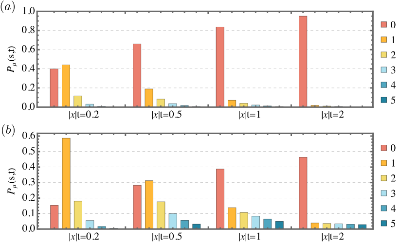
Figure 2: The early-time operator size distribution $P_{\mu}(s,t)$ for the model (3) with only $U_{1}$ and $U_{3}$ nonzero across different phases: (a) In the dissipative phase with $U_{1}=3U_{3}[n(1-n)]/2$, the operator weight rapidly decays to zero for $s\geq 1$. (b) In the scrambling phase with $U_{1}=U_{3}[n(1-n)]/2$, the operator weight at $s=0$ saturates to $P_{\mu}(0,\infty)=r=1/2$.

We further explore the fate of the scrambling transition in the low/high-density limit $n\rightarrow 0/1$. In this case, (32) is dominated by terms with the smallest $q$ or $\sum_{l}p$. For the dissipation process, we only keep $p_{1}+p_{2}=1$ and $p_{3}+p_{4}=1$ with strength $U_{1,0,0,1}\equiv U_{1}$. This represents a direct hopping between the system and the environment. The dominant scrambling process is given by $q=4$ or $\sum_{l}p_{l}=4$, which are four-fermion interactions. As an example, let us focus on a special term with $p_{1}+p_{2}=3$ and introduce its strength $U_{3}$. This corresponds to the interaction between three system fermion operators and one environment fermion operator. This environment propelled scrambling rate is proportional to $n(1-n)$ due to the Pauli blockade in the scattering process. This model is illustrated in FIG. 1, for which we have $\varkappa=U_{3}[n(1-n)]-U_{1}$, and the scrambling transition occurs at $U_{1}/U_{3}=n(1-n)$. We expect its scaling at $n\rightarrow 0/1$ to be exact in wider generic models.

To fully characterize the operator growth in this simplified model with only $U_{1}$ and $U_{3}$, we directly solve the differential equation (31). The result reads

$$Z_{\mu}(\nu,t)=1-\frac{(r-1)(1-e^{-\nu})}{e^{-\varkappa t}(r-e^{-\nu})-(1-e^{-\nu})}.$$ (33)

This takes the same form as the results of the Majorana model in Zhang and Yu (2023). Here, all density dependence is through $\varkappa$ and $r\equiv U_{1}/U_{3}[n(1-n)]$. Expanding in terms of $e^{-\nu}$, we obtain the operator size distribution

$$P_{\mu}(s,t)=\begin{cases}1-(1-r)\frac{e^{\varkappa t}}{e^{\varkappa t}-r},&(s=0)\\ (1-r)^{2}\frac{e^{\varkappa t}(e^{\varkappa t}-1)^{s-1}}{(e^{\varkappa t}-r)^{s+1}}.&(s\geq 1)\end{cases}$$ (34)

The dissipative phase corresponds to $r>1$ and $\varkappa<0$, where the operator size distribution decays exponentially in size $s$. For $|\varkappa|t\gtrsim 1$, the operator weight at $s>0$ also decays as $e^{\varkappa t}$ in time, approaching $P_{\mu}(s,\infty)=\delta_{s,0}$ in the long-time limit. As a comparison, the scrambling phase has $r<1$ and $\varkappa>0$. The operator size distribution is approximately constant for $1\leq s\lesssim e^{\varkappa t}$. In the long-time limit, we have $P_{\mu}(0,\infty)=r$, and there is always finite operator weight at $s>0$. We provide a density plot of $P_{\mu}(s,t)$ in both phases in FIG. 2.

VI Scrambling Phase at Late-time

In the scrambling phase, the growth of operator size saturates when the time $t$ greatly exceeds the scrambling time $t_{s}=\varkappa^{-1}\ln N$. In this section, we examine the operator size distribution in the late-time regime when $t\approx t_{s}$. Since a typical operator now has size $s\sim O(N)$, we take the continuum limit by introducing $\sigma=s/N\in[0,1]$ and $\mathcal{P}_{\mu}(\sigma,t)=NP_{\mu}(\sigma N,t)$ as in Majorana fermion systems Zhang and Yu (2023). As in the early-time calculation, it is convenient to introduce the generating function

$$\mathcal{S}_{\mu}(v,t)=\int_{0}^{1}d\sigma~{}\mathcal{P}_{\mu}(\sigma,t)e^{-\sigma v}=Z_{\mu}(v/N,t).$$ (35)

Due to the exponential growth factor $e^{\varkappa t}$ approaching order $N$, the traditional large-$N$ expansion becomes problematic. Consequently, Eq. (29) or (31) becomes invalid. To perform a resummation over all leading contributions for fixed $e^{\varkappa t}/N$, we employ the scramblon effective field developed in Refs. Gu et al. (2022); Stanford et al. (2022); Zhang and Gu (2023). The basic assumption is that these contributions arise due to out-of-time-ordered correlations mediated by a collective mode, known as the scramblon. This effective theory contains a set of Feynman rules for scramblons, which can be used to compute generic correlation functions. Firstly, a scramblon has an exponentially growing propagator

$$\leavevmode\hbox to64.76pt{\vbox to11.18pt{\text{[drawing]}}}=-\frac{e^{\varkappa t}}{C}\equiv-\lambda, t 0 t 0$$ (36)

which is a signature of quantum many-body chaos. Here, $C\propto N$ is a numerical factor. Secondly, scramblons can interact with a pair of fermion operators $\hat{c}_{j}$ and $\hat{c}_{j}^{\dagger}$, with scattering vertexes

$$\leavevmode\hbox to34.78pt{\vbox to29.29pt{\text{[drawing]}}}=\Upsilon^{R,m},\ \ \ \ \ \ \leavevmode\hbox to41.45pt{\vbox to29.29pt{\text{[drawing]}}}=\Upsilon^{A,m}.$$ (37)

Here, $m$ labels the number of scramblons, and $R/A$ denotes scattering in the past/future. Notice that we have not fixed the normalization of the scramblon field. There exists a transformation $C\rightarrow a^{2}C$ and $\Upsilon^{m}\rightarrow a^{m}\Upsilon^{m}$ that leaves all physical observables invariant. For systems with time-reversal symmetry (as our complex Brownian SYK model), we have $\Upsilon^{R,m}=\Upsilon^{A,m}=\Upsilon^{m}$. In particular, we have $\Upsilon^{0}=G^{W}(0,0)|_{\nu=0}=\sqrt{n(1-n)}$.

Let us first compute the generating function $\mathcal{S}_{\mu}(v,t)$ using these Feynman rules and postpone the determination of $C$ and $\Upsilon^{m}$. If we only keep out-of-time order correlations Gu et al. (2022), we can approximate

$$\mathcal{S}_{\mu}(v,t)\approx~{}_{\mu}\langle\hat{c}_{1}(t)|e^{-\frac{v}{N}\hat{S}_{\mu}^{\prime}}|\hat{c}_{1}(t)\rangle_{\mu},$$ (38)

with

$$\hat{S}_{\mu}^{\prime}=\sum_{j}{2A(\mu)}\Big{[} 2\sqrt{n(1-n)}-\hat{\xi}_{j}^{\dagger}\hat{c}_{j}-\hat{c}_{j}^{\dagger}\hat{\xi}_{j}\Big{]}.$$ (39)

Here, we retain cross terms between $(\hat{c},\hat{c}^{\dagger})$ and $(\hat{\xi},\hat{\xi}^{\dagger})$ as operators while replacing other terms with their expectation values on the reference state $|I\rangle_{\mu}$. We further represent $\mathcal{S}_{\mu}(v,t)$ using the path-integral approach:

$$\mathcal{S}_{\mu}=e^{-4A\sqrt{n(1-n)}v}\frac{\left<T_{\mathcal{C}}\,c^{u,2}_{1}(t)\overline{c}^{u,1}_{1}(t)e^{\frac{2Av}{N}\sum_{j}(\,c^{d,2}_{1}(0)\overline{c}^{d,1}_{1}(0)+\bar{c}^{d,2}_{1}(0)c^{d,1}_{1}(0))}\right>}{\sqrt{n(1-n)}},$$ (40)

We expand the source term in $\nu$, each insertion can create arbitrary number of scramblons, which interacts with $c^{u,2}_{1}(t)\overline{c}^{u,1}_{1}(t)$ in the future. Diagrammatically, we find

$$\mathcal{S}_{\mu}(v,t)= \leavevmode\hbox to65.85pt{\vbox to69.09pt{\text{[drawing]}}}=\frac{e^{-4A\sqrt{n(1-n)}v}}{\sqrt{n(1-n)}}\sum_{n=0}^{\infty}\frac{(4Av)^{n}}{n!}$$ (41)

$$\times\sum_{\{m_{j}\geq 0\}}\left(-\frac{e^{\varkappa t}}{C}\right)^{\sum_{j}m_{j}}\frac{\Upsilon^{\sum_{j}m_{j}}\Upsilon^{m_{1}}\ldots\Upsilon^{m_{n}}}{m_{1}!m_{2}!\ldots m_{n}!},$$

where we have used the fact that both $c^{d,2}_{1}(0)\overline{c}^{d,1}_{1}(0)$ and $\bar{c}^{d,2}_{1}(0)c^{d,1}_{1}(0)$ share the same scattering vertexes Zhang (2023) in our setup where the density matrix is equally split as shown in (24). In other words, $\Upsilon^{m}$ remains invariant under the particle-hole transformation. The summation can be carried out by introducing auxiliary functions $f(x)$ and $h(y)$ Gu et al. (2022), which satisfies

$$f(x)=\sum_{m=0}^{\infty}\frac{(-x)^{m}}{m!}\Upsilon^{m},\ \ \ \ \ \ f(x)=\int_{0}^{\infty}dy~{}h(y)e^{-xy}.$$ (42)

In particular, we have $f(0)=\Upsilon^{0}=\sqrt{n(1-n)}$. The summation in (41) gives

$$\mathcal{S}_{\mu}(v,t)=\int_{0}^{\infty}dy~{}\frac{h(y)}{\sqrt{n(1-n)}}e^{-4Av\left(\sqrt{n(1-n)}-f(\lambda y)\right)}.$$ (43)

Now, we determine $\Upsilon^{m}$ in the simplified model by comparing (43) with (33) in the early-time limit with $1\ll\varkappa t\ll\ln N$. Using $\eqref{eqn:resSmunut}$, we should expand $e^{\varkappa t}y/C$ to leading order, which gives

$$\mathcal{S}_{\mu}(v,t)=\frac{1}{\sqrt{n(1-n)}}f\left(\frac{4A(\mu)e^{\varkappa t}\Upsilon^{1}v}{C}\right).$$ (44)

On the other hand, expanding (33) for small $\nu=v/N$, we obtain

$$\mathcal{S}_{\mu}(v,t)=r+\frac{1-r}{1+e^{\varkappa t}v(1-r)^{-1}/N}.$$ (45)

To proceed, we use the aforementioned symmetry $C\rightarrow a^{2}C$ and $\Upsilon^{m}\rightarrow a^{m}\Upsilon^{m}$ to fix

$$\frac{4A(\mu)\Upsilon^{1}}{C}=\frac{1}{(1-r)N}.$$ (46)

In this convention, we have $f(x)=\sqrt{n(1-n)}[r+(1-r)/(1+x)]$, which corresponds to

$$\Upsilon^{0}=\sqrt{n(1-n)},\;\;\;\;\;\Upsilon^{m}=\sqrt{n(1-n)}(1-r)\,m!.$$ (47)

Using (46), this further gives $C/N=4(1-r)n(1-n)$. The scaling of $\Upsilon^{m}$ and $C$ in the low/high density limit matches their counterparts in closed Brownian SYK models Zhang (2023). We can also apply the inverse Laplace transform to $f(x)$ to determine

$$h(y)=\sqrt{n(1-n)}\left[(1-r)e^{-y}+r\delta(y)\right].$$ (48)

Using explicit expressions for both $f(x)$ and $h(y)$, the generating function reads

$$\mathcal{S}_{\mu}(v,t)=r+\int_{0}^{\infty}dy~{}(1-r)e^{-y}e^{-s_{\text{sc}}\frac{\lambda y}{1+\lambda y}},$$ (49)

where $s_{\text{sc}}=4n(1-n)(1-r)$. Performing the inverse Laplace transform, we find the continuum size distribution function $\mathcal{P}_{\mu}(\sigma,t)=r\delta(\sigma)+\mathcal{P}^{\text{r}}_{\mu}(\sigma,t)$, with

$$\mathcal{P}^{\text{r}}_{\mu}(\sigma,t) =\theta(s_{\text{sc}}-\sigma)\frac{s_{\text{sc}}(1-r)e^{\frac{\sigma}{\lambda(\sigma-s_{\text{sc}})}}}{\lambda(\sigma-s_{\text{sc}})^{2}}.$$ (50)

For systems at half-filling $n=1/2$ with $r=0$, the operator size distribution saturates to a delta function at $\sigma=s_{\text{sc}}=1$. This corresponds to the standard maximally scrambled operator in complex fermion systems, where each operator in (12) appears with the same probability, resulting in an average size of $1$. When $n\neq 1/2$, the Hilbert space restriction reduces the effective dimension of the operator space, and the saturation value becomes $4n(1-n)$, which diminishes as $n\rightarrow 0/1$. Introducing a finite $r$ further reduces $s_{\text{sc}}$ by a factor of $(1-r)$, indicating a “drag” force exerted by the environment, similar to the Majorana case Zhang and Yu (2023). Additionally, we have a singular part $r\delta(\sigma)$, representing the contribution of pure environment operators.

VII Summary

In this work, we investigate how charge conservation affects the environment-induced information scrambling transitions by examining a solvable complex Brownian SYK model embedded in an environment. After defining the size operator within our setup, we analyze the dominant processes in the low/high density limits. This analysis leads us to identify a minimal model featuring system-environment hopping, denoted as $U_{1}$, and four-fermion interactions, denoted as $U_{3}$. We determine that the scrambling transition occurs at $U_{1}/U_{3}=n(1-n)$, which separates a dissipative phase characterized by large $U_{1}$ from a scrambling phase characterized by small $U_{1}$. Furthermore, we delve into the late-time regime using the scramblon effective theory Gu et al. (2022); Stanford et al. (2022), revealing the renormalization of maximally scrambled operators with a typical size of $4n(1-n)(1-r)$.

Acknowledgment. This project is supported by the Key Area Research and Development Program of Guangdong Province (Grant No. 2019B030330001), the National Natural Science Foundation of China (Grant No. 12374477 and No. 12074440), and Guangdong Project (Grant No. 2017GC010613).

References

• Hayden and Preskill (2007) P. Hayden and J. Preskill, JHEP 09, 120 (2007), eprint 0708.4025.
• Sekino and Susskind (2008) Y. Sekino and L. Susskind, JHEP 10, 065 (2008), eprint 0808.2096.
• Shenker and Stanford (2015) S. H. Shenker and D. Stanford, JHEP 05, 132 (2015), eprint 1412.6087.
• Roberts et al. (2015) D. A. Roberts, D. Stanford, and L. Susskind, JHEP 03, 051 (2015), eprint 1409.8180.
• Islam et al. (2015) R. Islam, R. Ma, P. M. Preiss, M. Eric Tai, A. Lukin, M. Rispoli, and M. Greiner, Nature (London) 528, 77 (2015), eprint 1509.01160.
• Li et al. (2017) J. Li, R. Fan, H. Wang, B. Ye, B. Zeng, H. Zhai, X. Peng, and J. Du, Phys. Rev. X 7, 031011 (2017), eprint 1609.01246.
• Gärttner et al. (2017) M. Gärttner, J. G. Bohnet, A. Safavi-Naini, M. L. Wall, J. J. Bollinger, and A. M. Rey, Nature Phys. 13, 781 (2017), eprint 1608.08938.
• Brydges et al. (2019) T. Brydges, A. Elben, P. Jurcevic, B. Vermersch, C. Maier, B. P. Lanyon, P. Zoller, R. Blatt, and C. F. Roos, Science 364, 260 (2019), eprint 1806.05747.
• Sánchez et al. (2019) C. M. Sánchez, A. K. Chattah, K. X. Wei, L. Buljubasich, P. Cappellaro, and H. M. Pastawski, arXiv e-prints arXiv:1902.06628 (2019), eprint 1902.06628.
• Landsman et al. (2019) K. A. Landsman, C. Figgatt, T. Schuster, N. M. Linke, B. Yoshida, N. Y. Yao, and C. Monroe, Nature (London) 567, 61 (2019), eprint 1806.02807.
• Joshi et al. (2020) M. K. Joshi, A. Elben, B. Vermersch, T. Brydges, C. Maier, P. Zoller, R. Blatt, and C. F. Roos, Phys. Rev. Lett.  124, 240505 (2020), eprint 2001.02176.
• Blok et al. (2021) M. S. Blok, V. V. Ramasesh, T. Schuster, K. O’Brien, J. M. Kreikebaum, D. Dahlen, A. Morvan, B. Yoshida, N. Y. Yao, and I. Siddiqi, Phys. Rev. X 11, 021010 (2021), eprint 2003.03307.
• Domínguez et al. (2021) F. D. Domínguez, M. C. Rodríguez, R. Kaiser, D. Suter, and G. A. Álvarez, Phys. Rev. A 104, 012402 (2021), eprint 2005.12361.
• Domínguez and Álvarez (2021) F. D. Domínguez and G. A. Álvarez, Phys. Rev. A 104, 062406 (2021), eprint 2107.03870.
• Mi et al. (2021) X. Mi et al., Science 374, abg5029 (2021), eprint 2101.08870.
• Cotler et al. (2022) J. Cotler, T. Schuster, and M. Mohseni (2022), eprint 2208.02256.
• Sánchez et al. (2022) C. M. Sánchez, A. K. Chattah, and H. M. Pastawski, Phys. Rev. A 105, 052232 (2022), eprint 2112.00607.
• Nahum et al. (2018) A. Nahum, S. Vijay, and J. Haah, Phys. Rev. X 8, 021014 (2018), eprint 1705.08975.
• Qi and Streicher (2019) X.-L. Qi and A. Streicher, JHEP 08, 012 (2019), eprint 1810.11958.
• von Keyserlingk et al. (2018) C. von Keyserlingk, T. Rakovszky, F. Pollmann, and S. Sondhi, Phys. Rev. X 8, 021013 (2018), eprint 1705.08910.
• Khemani et al. (2018a) V. Khemani, A. Vishwanath, and D. A. Huse, Phys. Rev. X 8, 031057 (2018a), eprint 1710.09835.
• Hunter-Jones (2018) N. Hunter-Jones (2018), eprint 1812.08219.
• Chen and Lucas (2021) C.-F. Chen and A. Lucas, Commun. Math. Phys. 385, 1273 (2021), eprint 1905.03682.
• Lucas (2019) A. Lucas, Phys. Rev. Lett. 122, 216601 (2019), URL https://link.aps.org/doi/10.1103/PhysRevLett.122.216601.
• Chen et al. (2020a) X. Chen, Y. Gu, and A. Lucas, SciPost Phys. 9, 071 (2020a), eprint 2007.10352.
• Lucas and Osborne (2020) A. Lucas and A. Osborne, J. Math. Phys. 61, 122301 (2020), eprint 2007.07165.
• Yin and Lucas (2021) C. Yin and A. Lucas, Phys. Rev. A 103, 042414 (2021), eprint 2010.06592.
• Zhou and Swingle (2021) T. Zhou and B. Swingle (2021), eprint 2112.01562.
• Dias et al. (2021) B. C. Dias, M. Haque, P. Ribeiro, and P. McClarty (2021), eprint 2102.09846.
• Wu et al. (2021) Y. Wu, P. Zhang, and H. Zhai, Physical Review Research 3, L032057 (2021), eprint 2011.07698.
• Gu et al. (2022) Y. Gu, A. Kitaev, and P. Zhang, JHEP 03, 133 (2022), eprint 2111.12007.
• Zhang and Gu (2023) P. Zhang and Y. Gu, JHEP 10, 018 (2023), eprint 2212.04358.
• Liu and Zhang (2024) Z. Liu and P. Zhang, Phys. Rev. Lett. 132, 060201 (2024), eprint 2306.05678.
• Gao et al. (2023) Q. Gao, P. Zhang, and X. Chen (2023), eprint 2310.07043.
• Gao et al. (2024) Q. Gao, T. Zhou, P. Zhang, and X. Chen (2024), eprint 2403.03457.
• Zhang and Yu (2023) P. Zhang and Z. Yu, Phys. Rev. Lett. 130, 250401 (2023).
• Bhattacharya et al. (2022) A. Bhattacharya, P. Nandy, P. P. Nath, and H. Sahu (2022), eprint 2207.05347.
• Liu et al. (2022) C. Liu, H. Tang, and H. Zhai, arXiv e-prints arXiv:2207.13603 (2022), eprint 2207.13603.
• Schuster and Yao (2022) T. Schuster and N. Y. Yao (2022), eprint 2208.12272.
• Weinstein et al. (2022) Z. Weinstein, S. P. Kelly, J. Marino, and E. Altman (2022), eprint 2210.14242.
• Kitaev (2015) A. Kitaev, A simple model of quantum holography (2015).
• Maldacena and Stanford (2016) J. Maldacena and D. Stanford, Phys. Rev. D 94, 106002 (2016), eprint 1604.07818.
• Kitaev and Suh (2018) A. Kitaev and S. J. Suh, JHEP 05, 183 (2018), eprint 1711.08467.
• Saad et al. (2018) P. Saad, S. H. Shenker, and D. Stanford (2018), eprint 1806.06840.
• Sünderhauf et al. (2019) C. Sünderhauf, L. Piroli, X.-L. Qi, N. Schuch, and J. I. Cirac, JHEP 11, 038 (2019), eprint 1908.00775.
• Larkin and Ovchinnikov (1969) A. I. Larkin and Y. N. Ovchinnikov, Soviet Journal of Experimental and Theoretical Physics 28, 1200 (1969).
• Kitaev (2014) A. Kitaev, in Talk given at the Fundamental Physics Prize Symposium (2014), vol. 10.
• Rakovszky et al. (2018) T. Rakovszky, F. Pollmann, and C. W. von Keyserlingk, Phys. Rev. X 8, 031058 (2018), URL https://link.aps.org/doi/10.1103/PhysRevX.8.031058.
• Khemani et al. (2018b) V. Khemani, A. Vishwanath, and D. A. Huse, Phys. Rev. X 8, 031057 (2018b), URL https://link.aps.org/doi/10.1103/PhysRevX.8.031057.
• Huang (2019) Y. Huang, arXiv e-prints arXiv:1902.00977 (2019), eprint 1902.00977.
• Rakovszky et al. (2019) T. Rakovszky, F. Pollmann, and C. W. von Keyserlingk, Phys. Rev. Lett.  122, 250602 (2019), eprint 1901.10502.
• Chen et al. (2020b) X. Chen, Y. Gu, and A. Lucas, SciPost Phys. 9, 071 (2020b), URL https://scipost.org/10.21468/SciPostPhys.9.5.071.
• Zhang (2023) P. Zhang, JHEP 04, 105 (2023), eprint 2301.03189.
• Agarwal and Xu (2020) L. Agarwal and S. Xu, JHEP 22, 045 (2020), eprint 2108.05810.
• Stanford et al. (2022) D. Stanford, Z. Yang, and S. Yao, JHEP 02, 200 (2022), eprint 2107.10252.
• Chen et al. (2017) Y. Chen, H. Zhai, and P. Zhang, JHEP 07, 150 (2017), eprint 1705.09818.
• Zhang (2019) P. Zhang, Phys. Rev. B 100, 245104 (2019), eprint 1909.10637.
• Almheiri et al. (2019) A. Almheiri, A. Milekhin, and B. Swingle (2019), eprint 1912.04912.
• Zhang et al. (2020) P. Zhang, Y. Gu, and A. Kitaev, JHEP 21, 094 (2020), eprint 2012.01620.
• Roberts et al. (2018) D. A. Roberts, D. Stanford, and A. Streicher, JHEP 06, 122 (2018), eprint 1802.02633.
• Aleiner et al. (2016) I. L. Aleiner, L. Faoro, and L. B. Ioffe, Annals of Physics 375, 378 (2016).