Patching-based Deep Learning model for the Inpainting of Bragg Coherent Diffraction patterns affected by detectors’ gaps

Abstract

We propose a deep learning algorithm for the inpainting of Bragg Coherent Diffraction Imaging (BCDI) patterns affected by detector gaps. These regions of missing intensity can compromise the accuracy of reconstruction algorithms, inducing artifacts in the final result. It is thus desirable to restore the intensity in these regions in order to ensure more reliable reconstructions. The key aspect of our method lies in the choice of training the neural network with cropped sections of both experimental diffraction data and simulated data and subsequently patching the predictions generated by the model along the gap, thus completing the full diffraction peak. This provides us with more experimental training data and allows for a faster model training due to the limited size, while the neural network can be applied to arbitrarily larger BCDI datasets. Moreover, our method not only broadens the scope of application but also ensures the preservation of data integrity and reliability in the face of challenging experimental conditions.

1 Introduction

Coherent Diffraction Imaging (CDI) is a lens-less technique that exploits scattering of a coherent X-ray beam to study nano-particles with high spatial resolution [1, 2, 3]. The resulting diffraction pattern contains information about the three-dimensional (3D) electron density distribution in the material. However, since the phase information is lost during the measurement, iterative algorithms are needed to reconstruct the real-space object. This procedure, referred to as phase retrieval (PR), normally entails alternated projections between direct and reciprocal space, and the application of constraints in both spaces such that the algorithm converges towards the solution [4, 5, 6, 7, 8].

In case of crystalline samples, Bragg Coherent Diffraction Imaging (BCDI) allows to measure the internal strain of particles ranging in size from few micrometers down to 20 nm [9, 10, 11, 12]. BCDI enables to observe the strain evolution in situ during gas reactions [13, 14], in electrochemical environment [15, 16] or to observe the particle modifications over temperature variations [17]. These reactions often occur at the surface of the nano-particles, thus a good spatial resolution is required in order to follow their evolution by monitoring the effects at the particles’ surface. Since the measured intensity ($\mathbf{I}$) corresponds to the squared modulus of the object Fourier Transform (FT), the real-space resolution is inversely proportional to the extent of the recorded diffraction pattern. Consequently, there is a requirement for detectors with large sensing areas to achieve high resolution. [18].

Standard photon counting detectors are usually assembled out of pixelated chips separated by insensitive gaps. These gaps consist of a few pixel-wide lines, whose size varies according to the detector model. For example, the photon-counting MAXIPIX detector contains a cross-shaped six pixel-wide gap [19] while the Eiger2M detector [20], having a larger sensing area, has both 12 and 38 pixel-wide gaps. Technological solutions are on the horizon, e.g. the PIMEGA or through silicon via technology [21], but the majority of pixel detectors available at the time of writing have gaps between active areas.

The acquisition of the 3D BCDI pattern is obtained by rotating the sample and by stacking each 2D detected image for each rotation angle. This implies that the gap lines in each 2D image turn into gap planes of empty pixels in the full 3D pattern.

The effect of these regions of missing intensity on the recorded diffraction is the corruption of the PR algorithms that eventually leads to the presence of artifacts in the reconstructed real-space object [22] (see Supplementary Figure 1). These artefacts become more significant as the BCDI 3D array is large, thus severely limiting the reconstructed object resolution.

Here, we propose to preprocess the 3D experimental BCDI data affected by these gaps using a Deep Learning (DL) inpainting method. Our model is able to make consistent predictions of the in-gap intensity on experimental BCDI data, thus reducing artifacts in the reconstructed object.

Image inpainting has been widely explored in the field of photography and image processing for the restoration of damaged pictures. Many techniques have been developed, from classical polynomial interpolations to more advanced techniques such as diffusion-based methods or sparse representation methods [23]. More recently image inpainting has been addressed with the use of deep convolutional neural networks which have shown promising and accurate results in different fields [24].

In the field of Coherent Diffraction Imaging, and more specifically BCDI, deep learning methods have been exploited for defect identification, classification [25, 26], and for phase retrieval [27, 28, 29]. Image inpainting using DL for X-ray diffraction imaging has already been successfully tested by Bellisario et al. [30] on 2D simulated data and by Chavez et al. [31] on 2D X-ray scattering images. However, a recurrent problem in DL for BCDI is the lack of a large experimental dataset, thus the need to train the model using mostly simulated diffraction data. This limitation often biases the DL models that eventually yield poor results on experimental data. Moreover, these DL models use a fixed input-output size which is inconvenient for practical use since typical experimental BCDI data are cropped and centered during preprocessing, leading to possible different array size each time.

Here, we propose a solution that solves both the limited experimental dataset as well as the size constraint issues for the case of detector gap inpainting through the implementation of a “patching model” trained on small 32$\times$32$\times$32 pixel-size cropped portions ($\mathbf{P}$) of the diffraction patterns. This patching technique allows to use a large number of small portions from experimental BCDI data along with simulated ones. Henceforward, we can use a much lighter and rapidly trainable DL network. Our model can then be applied on large BCDI 3D array, regardless of the data size. The size of $\mathbf{P}$ was chosen such as it was larger than the usual gap size and the finite size oscillations of the intensity pattern.

2 Results

2.1 Dataset preparation

The dataset used to train the model contains a mix of simulated and experimental Bragg Coherent Diffraction patterns. Experimental data (ED) were taken from measurements performed at the ID01 beamline of The European Synchrotron (ESRF, in Grenoble, France) [32]. Simulated data (SD) have been constructed following the procedure described in Ref. [25], i.e. creating 3D face-centered-cubic (FCC) crystals from random atomic elements, crystal shapes and sizes, followed by an energy relaxation using LAMMPS [33]. The 128$\times$128$\times$128 pixel-size BCDI diffraction pattern of the (200) Bragg peak was then calculated using the PyNX package [34] with random particle orientation as well as reciprocal space step size, i.e. different oversampling ratio. However, the resulting SD are still very different compared to what was measured experimentally and could bias our DL model, diminishing its applicability to experimental data. To prevent this, we modified the SD by introducing noise in both reciprocal and real space as detailed in Supplementary section S2.

From each entire diffraction pattern, 10 portions $\mathbf{P}$ of 32$\times$32$\times$32 pixel-size have been cropped out pseudo-randomly, see Fig. 1. Having noticed poorer accuracy for the prediction around low intensity regions, portions from peripheral areas have been preferentially selected over the center of the peak. Thus the final dataset, composed of 50% ED and 50% SD, contains 30,000 of these small portions.

2.2 Data preprocessing

During the DL model training, an artificial vertical mask of zero intensity pixels, and of fixed size, was added in the middle of each single portion $\mathbf{P}$, as defined above, in order to simulate the presence of the detector gap (Fig. 1b). To include the case of cross-shaped gaps, an additional mask, of equivalent size, was applied horizontally at a random position to a certain subset of the training data (see the last example in Fig. 1b).

The last preprocessing step transforms the data to a logarithmic scale and normalises each image between 0 and 1 in order to avoid overfitting high-intensity regions over the low-intensity ones. The masked images were then used as model input while the ground truth unmasked images were used in the calculation of the loss function, as a comparison with the DL predictions.

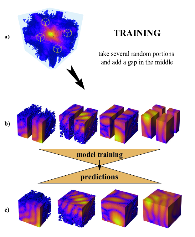
Figure 1: Sketch of the data processing and DL model training. a Large BCDI data where small 32$\times$32$\times$32 pixel-size portions are randomly selected. b Small portions in renormalized log scale and artificially masked with zeros to simulate detector’s gaps and used as input of the DL model. c DL model predictions for the corresponding masked inputs with the inpainted gap.

2.3 Network architecture and training

The adopted DL model was based on the U-Net architecture [35], see Figure 2. It consists of two main blocks, namely the encoder and the decoder. The encoder is composed of 4 convolutional layers followed by MaxPooling and leads to a reduction of the data array size from 32$\times$32$\times$32 down to 2$\times$2$\times$2. The decoder section uses other convolutional and UpSampling layers to enlarge the array back to its original size. Information is transferred between each encoder and decoder layers through skip connections, ensuring an easier search for the loss function’s absolute minimum [36]. All encoder and decoder layers use the Leaky ReLU activation function with a slope of 0.2 for negative inputs. Finally, 3 additional convolutional layers are added after the decoder as a way to avoid image smoothing by the array expansion in the decoder. The sigmoid activation function is used as last layer in order to bound the output values between 0 and 1, for the model outputs to have the same intensity range as the inputs. To improve the receptive field of the first convolutional layers and thus provide higher long-range correlation understanding in the feature extraction, dilated convolutions have been employed with variable dilation rate [37]. More precisely, as depicted in Fig. 2, in the first two encoder blocks the input was concatenated with four different convolutions of itself, each one with a different dilation rate (the d parameter in Fig.2). Standard convolutional layers were used in last two encoder blocks as the size of the inputs was already small enough to be treated with normal convolutional layers and a 3$\times$3$\times$3 pixel-size kernel.

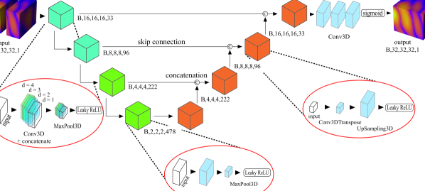
Figure 2: Architecture of the deep learning model. A modified U-Net architecture with the use of dilated convolutions in the first two encoder blocks (left red circle) where the input was concatenated to its convolutions with different dilation rates ($d$ parameter) before the MaxPooling layer. The gap-affected small portions $\mathbf{P}$, in batches (B) of 32, were used as input (top left) and progressively sent through the encoder section down to a small volume of 2x2x2 pixels. Each building block of the decoder section (orange cubes) takes as input the concatenation of its previous block’s output with the corresponding output of the encoder block of the the same size. The final output (top right) being a batch of inpainted $\mathbf{P}$.

The network was built using the Tensorflow python library [38] and was trained for 100 epochs, with ADAM optimizer [39] starting with a learning rate of 10^-3 decreasing progressively using the ReduceLROnPlateau callback available in Tensorflow. The shuffled 30,000 small portions dataset was split into a training (93.5%), validation (4%) and test (2.5%) sets. Batches of 32 images were used and training and validation losses were monitored at each epoch in order to avoid overfitting to the training dataset. Inpainted output and ground truth regions were compared using a custom loss function consisting in the sum of three main terms, namely: a Mean Absolute Error (MAE), a Structural Similarity Index perceptual loss [40], and a MAE on the image gradients.

To assess the DL model performances we used the Pearson Correlation Coefficient (PCC). This coefficient measures the linear correlation between two images and in our specific case yields an estimation of the similarity between the DL prediction and the corresponding ground truth, thus an indication of the predictive accuracy of the model. It is defined by the following:

$$PCC=\frac{\sum_{i\in\text{gap}}(\textbf{P}_{i}^{\text{true}}-\langle\textbf{P}^{\text{true}}\rangle)(\textbf{P}_{i}^{\text{pred}}-\langle\textbf{P}^{\text{pred}}\rangle)}{\sqrt{\sum_{i\in\text{gap}}(\textbf{P}_{i}^{\text{true}}-\langle\textbf{P}^{\text{true}}\rangle)^{2}}\sqrt{\sum_{i\in\text{gap}}(\textbf{P}_{i}^{\text{pred}}-\langle\textbf{P}^{\text{pred}}\rangle)^{2}}},$$ (1)

where $\mathbf{P}^{\text{true}}$ was the 32$\times$32$\times$32 pixel-size ground truth portion in log scale without gap and $\mathbf{P}^{\text{pred}}$ was the same portion where the gap region was inpainted using our DL model. The $\langle\rangle$ symbol corresponds to the average over the gap. We note that the PCC for identical images was equal to 1.

Table 1 shows the average PCC values over a batch of 1000 samples of small portions from experimental BCDI data (where gaps have been artificially added). Vertical gaps of different sizes are considered. As expected, the accuracy decreases when the gap size increases since the prediction of the in-gap fringes becomes more and more difficult. Examples of DL predictions on small BCDI regions with a 6 pixels gap are shown in Supplementary Figs. 7 and 8 for respectively simulated and experimental data, demonstrating accurate in-gap intensity prediction.

Table 1: Average DL model accuracy on 32$\times$32$\times$32 pixel-size small BCDI portions over a batch of 1000 samples. The accuracy decreases as the gap size increases.

Gap size (pixels)	3	6	9	12
Pearson Correlation Coefficient	0.989	0.977	0.955	0.946

2.4 Results in reciprocal space

In order to make a prediction of the in-gap intensity of a large 3D BCDI array of arbitrary size, we use a “patching” method. A 32$\times$32$\times$32 pixel-size portion $\mathbf{P}$ centered around the gap of the large image was used as the DL model input and the in-gap intensity was predicted in this region. $\mathbf{P}$ was then repeatedly shifted by 1 pixel at a time along the gap and the prediction was calculated again, until the whole gap intensity was reconstructed. The final step involves averaging the overlapping predicted pixels, which contributes to robust DL predictions even when applied to experimental data. This averaging process helps mitigate potential prediction errors by smoothing them out.

However, this method can be time consuming as a prediction for a cross-shaped gap on 128$\times$128$\times$128 pixel-size BCDI data can take up to 12 minutes. To speed up this process, one can shift $\mathbf{P}$ by more than 1 pixel at a time, drastically decreasing the prediction time down to 1m30s for 4 skipped pixels, without significantly worsening the accuracy. More details on this skip method are available in Section 5 of the Supplementary information.

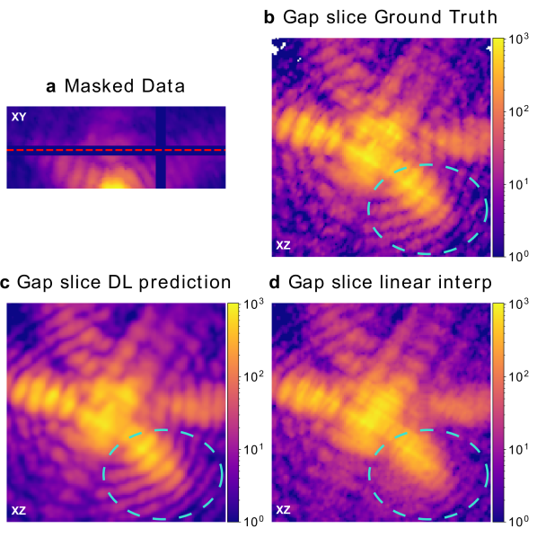
Figure 3: In-gap slice comparison between DL prediction and standard interpolation on experimental BCDI data. a 3D experimental BCDI data masked with a cross-like 6 pixel-wide gap - the red dotted line shows the location of the perpendicular ‘in-gap slices’ shown in b, c, d. In-gap slice b ground truth, c DL model prediction, d standard linear-interpolation using pixels immediately around the gap. Only our DL model was able to restore the correct fringes pattern as highlighted by the turquoise dashed circles.

In order to test the DL model accuracy on large BCDI data, we use the patching method on a large experimental BCDI array where a handmade 6 pixel-wide cross-shaped gap was added. Figure 3a displays the position of the gap in the XY plane while Fig. 3b shows the ground-truth in-gap intensity in the XZ plane. Our DL model prediction is shown in Fig. 3c, where the fringes pattern was accurately reproduced. One can notice that the ”grainy” features of the ground-truth are not reproduced due to the intrinsic denoising effect induced by the model training process [41].

As a comparison, a standard linear interpolation (LI) is shown in Fig. 3d. The cubic and nearest-neighbour interpolations are illustrated in Supplementary Fig. 9.

An improvement of the result from the DL model with respect to standard interpolation algorithms was observed in all the cases, in particular when comparing the fringes pattern in the bottom left of Figs. 3c and d. Where LI fails to reproduce the oscillations, DL succeeds. This was expected, since standard interpolations algorithms have no a priori knowledge of the oscillatory nature of diffraction fringes.

This is further demonstrated in Fig. 4 where the in-gap intensity is shown in the XY plane for a gap size of 12 pixels. The DL algorithm (Fig. 4b) was able to predict the correct fringes curvature across the gap. On the other hand, the standard interpolations (see Figs. 4c-d-e) neglect this curvature and reproduce straight oscillations perpendicular to the edges of the gap region.

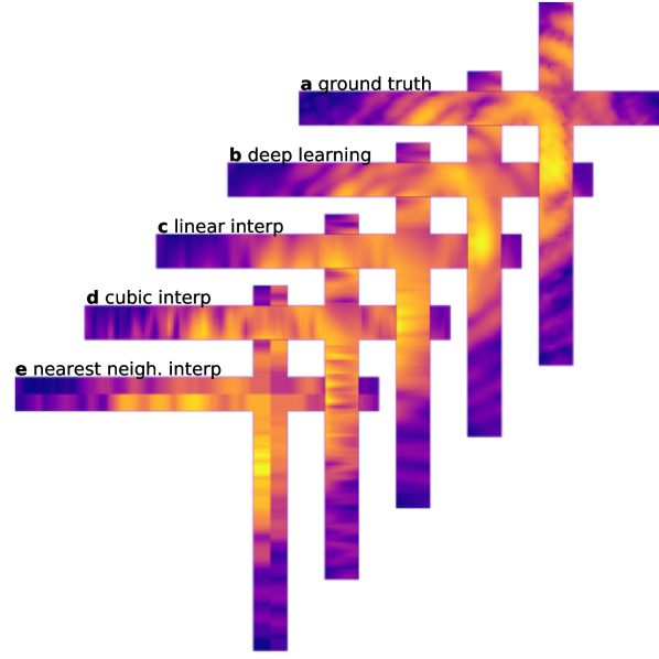
Figure 4: Comparison between DL prediction and several standard interpolations across the gap. a Ground truth intensity in the 12 pixel-wide cross-shaped gap (only the gap area is shown). b DL prediction. c, d, e respectively linear, cubic and nearest-neighbour interpolation. Only the DL model was able to recover the accurate fringes curvature across the gap.

2.5 Performances assessment

In this section we discuss the accuracy of our model with respect to: (i) the amount of intensity inside the cropped portion $\mathbf{P}$ and (ii) the oversampling ratio. In order to assess the model accuracy for the first case, we used a 128$\times$128$\times$128 pixel-size experimental diffraction pattern and we randomly cropped out 1000 portions $\mathbf{P}$ of 32$\times$32$\times$32 pixels. A vertical gap was placed in the middle of each $\mathbf{P}$ and the DL model was used to predict the in-gap intensity. The PCC accuracy as given in Table 1 was then calculated for each $\mathbf{P}$ individually and its average is shown as function of the average photon count in $\mathbf{P}$ (see Fig. 5). Lower PCC scores are obtained when the average intensity in the region is smaller, which is expected as the absence of significant features, that are lost in the Poisson noise, prevents accurate DL prediction. Moreover, as expected, from Fig. 5 emerges that the smaller the gap size, the better the accuracy of the prediction.

In order to compute the model accuracy as function of the oversampling ratio, we simulate BCDI arrays of the same region for different oversampling ratios (ORs) as shown in Figs. 6 a-b. Since a different OR implies different array size, comparing the model accuracy is not straightforward. To do so, we make the prediction of the full image using the method illustrated in Supplementary Fig. 13. For each OR, a vertical gap mask was applied to the whole BCDI array and the DL prediction was calculated. The gap was then shifted and this procedure was repeated until the whole BCDI array was predicted using our model, thus leading to a full BCDI predicted image. The PCC shown in Fig. 6c was then calculated using the whole BCDI array for different ORs and model gap sizes. As expected, the predictions are more accurate for large ORs and small gap sizes (i.e., large oscillation periods relative to the gap width). Some prediction examples are given in Supplementary Fig. 14.

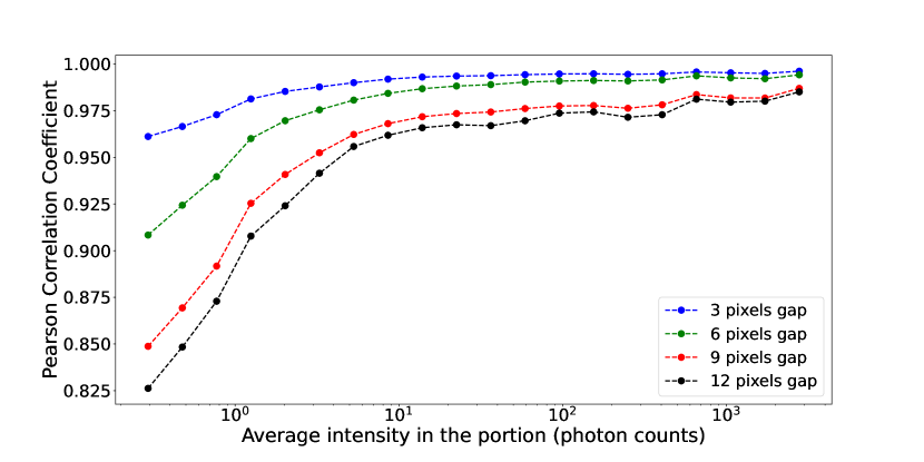
Figure 5: Prediction accuracy vs average intensity in cropped portion. The model prediction becomes more accurate as the overall intensity inside the considered portion increases. Conversely, in cases of low photon counts - indicating a prevalence of noise within the portion—the predictions were more prone to inaccuracies.

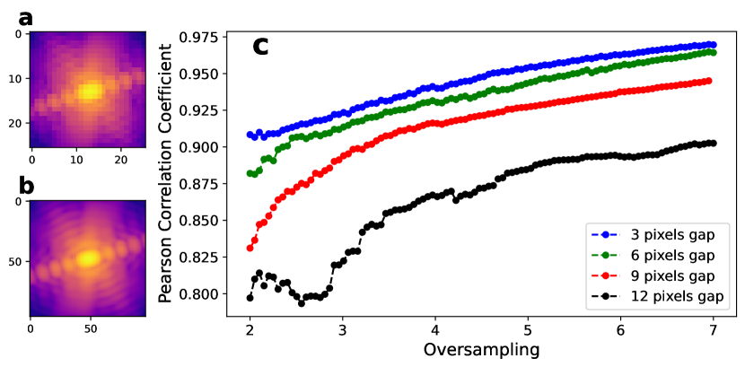
Figure 6: Prediction accuracy vs oversampling. a Low and b high oversampling simulated BCDI array of the same region. c Prediction accuracy as function of BCDI oversampling ratio for different gap size.

2.6 Reconstructions in real-space

2.6.1 Simulated real-space result

Since the final goal of the BCDI technique, before physical analysis, is the reconstruction of the real-space complex object, we assess here the reconstructed object quality before and after DL gap inpainting. A simulated BCDI array was used starting from a reconstruction by Carnis et al. [22]. After the reconstruction from experimental diffraction pattern, the real space phase of the particle was artificially set to zero (see Figures 7a-b), making the evaluation of the gap effect easier. From this reference “ground truth” object $\mathbf{O}$, the simulated diffracted amplitude correspond to $\mathbf{A}=\text{FT}\left[\mathbf{O}\right]$, where FT is the Fourier transform.

A 9 pixel-wide cross-shaped gap mask was then applied to $\mathbf{A}$ (see Supplementary Fig. 19b) and the corresponding real space object was calculated from the inverse FT (Figs. 7c-d). The presence of the gap in the diffraction pattern induces artefacts in real-space manifesting as non-zero module values outside the support region along the directions perpendicular to the gap planes (Fig. 7c). Most importantly, the gap induces variations in the object phase, and thus the reconstructed displacement field and strain [42], especially near the sample surfaces (Fig. 7d). Here, a phase variation of $\pm$0.2 radians is observed in Fig. 7d resulting in an error of $\pm$7pm in the lattice displacement field for the (111) Pt reflection. These artefacts are particularly problematic in the cases of (electro-)catalytic experiments [16] or in-situ gas experiments [43, 44, 45, 46, 14] where the chemical reactions occur at the nano-particle’s surfaces and can be studied by following the strain evolution in these regions. The presence of a large gap, or a gap close to the centre of the Bragg peak, could lead to a physical misinterpretation from a poorly reconstructed phase.

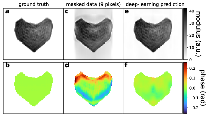
Figure 7: DL inpainting result on real-space object reconstruction. a-b Central slice of the ground truth object modulus and phase obtained from a simulated diffraction pattern with no gap. c-d Reconstruction with a 9 pixel-wide cross-like gap affected diffraction pattern. e-f Reconstruction after DL gap inpainting, drastically reducing the artefacts induced by the gap. The corresponding diffraction patterns are available in Supplementary Fig. 15. Note that in this example the phase of the ground truth object has been artificially set to zero (contrary to Fig. 8) for an easier comparison.

Afterwards, our DL model was used to predict the in-gap masked intensity (see Supplementary Fig. 15c), and the corresponding object was computed via the inverse FT using the ground truth reciprocal space phase (Figs. 7e-f). The artefacts on the reconstructed modulus disappear almost entirely. Furthermore, the reconstructed phase standard deviation is five times lower than the one calculated for the case with a gap and does not present any large variations close to the surfaces, showing that our DL method is suitable for the object reconstruction.

Referring to the work of Carnis et al. in Ref. [22], we evaluate the Root Mean Squared Error (RMSE) values of the strain for the particle in Supplementary Fig. 18 for different gap sizes. The wider the gap, the larger the variation from the mean, hence the less precise is the obtained strain distribution. However, it is clearly visible from the same figure that the restoration of the diffraction intensity using our DL method significantly reduces the error on the strain calculation. Also note that the mean value of the strain obtained from masked diffraction patterns differs from the expected zero, as depicted in Supplementary Fig. 17.

2.6.2 Experimental real-space result

In order to obtain a nano-particle reconstruction with high spatial resolution, one generally has to measure a relatively large BCDI array. With typical photon counting detectors, this leads to a region with a large gap as shown in Supplementary Fig. 1a. One common solution is to run the Phase Retrieval (PR) algorithms leaving the in-gap pixels free. However, with this approach PR algorithms often overestimate the intensity distribution inside the gap, leading to strong oscillation artefacts in the phase and strain of the reconstructed object as shown in Fig. 8b.

On the other hand, by inpainting the gap with our DL model before the PR (Fig.8a), the resulting strain map in Fig. 8c does not show any of these artefacts anymore, indicating that the in-gap prediction is accurate. Furthermore, we tested other methods for a comparison, namely: leaving pixels free only at the streaks position and setting the in-gap intensity to 0. The results are depicted in Supplementary Figs. 19-20-21, and show that DL inpainting is the best way to obtain a reliable high-resolution reconstruction from BCDI data with gaps. A second high-resolution example is shown in Supplementary Fig. 22.

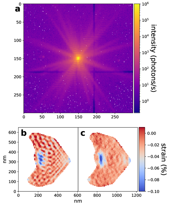
Figure 8: DL inpainting result on high-resolution experimental data containing a real gap. a DL inpainted high-resolution BCDI experimental array containing a real gap. b Object strain reconstruction leaving in-gap pixels free during PR. c Reconstructed strain using DL inpainted gap. The strong oscillation artefacts visible in b are removed by the DL inpainting.

2.7 Fine Tuning

There may be cases in which the DL model does not yield satisfactory predictions inside the gap, such as when the target image is too different from the training dataset, as shown in Fig. 9b. To overcome these situations, it is possible to fine-tune the model using a specific dataset obtained only from the target image. Our approach involves a secondary short training phase for the model, conducted on a limited dataset (6400 portions) derived from a random sub-sampling of the same 3D diffraction pattern affected by gaps that we aim to restore. This training exclusively uses portions of the detector that remain unaffected by gaps. The second training occurs typically within 2 to 5 epochs and usually takes up to one or two minutes.
By performing this fine-tuning, the model is biased on purpose to operate with specific features of the interested image (oversampling, particle shape, detector, etc) thus improving the performance on the real gap prediction (see Fig. 9c). We emphasize that this fine-tuning procedure is only advised when the prediction obtained with the pre-trained model is relatively poor.

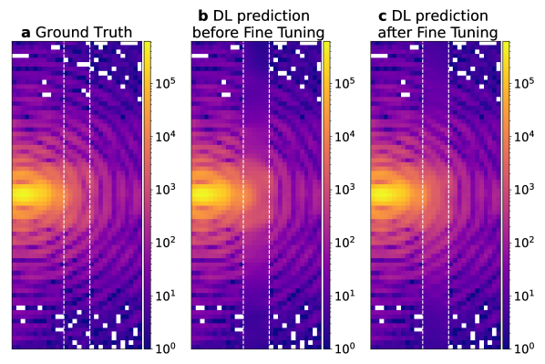
Figure 9: Fine Tuning. a The central slice of an experimental diffraction pattern in log scale. An artificial 6 pixel-wide vertical gap was added in the region between the two white dashed lines. b The corresponding slice after DL inpainting where the fringes pattern is not correctly retrieved. c The same slice of the inpainted image after 2 epochs of fine-tuning of the DL model. The fringes pattern was more reliably recovered.

3 Conclusion

In the present work, a Deep-Learning based approach for inpainting 3D BCDI arrays affected by a detector gap is proposed. The key point of our method is the use of a “patching” technique where only small portions of the BCDI arrays are used during training. This technique offers several benefits, namely: (i) it effectively removes the constraint on the size of the BCDI array, meaning that there is no need to train different models for different array sizes; (ii) given the small volume of the portions, the training of the model is faster and most importantly (iii) cropping small portions of large data leads to a drastic increase of the amount of experimental data available during the training, removing possible biases that often occur using only a simulated dataset. Our model achieves high accuracy on experimental BCDI data and was able to remove possible reconstruction artefacts on the real-space object, especially in the case of high-resolution BCDI data.

This deep learning “patching” approach could be applied to other imaging techniques with missing pixel problems and a lack of a large experimental training datasets, such as CDI, ptychography or any other techniques with image spatial correlations.

Supplementary information Supplementary information is available for this paper.

Declarations

• Funding:
  This project has been partly funded by the European Union’s Horizon 2020 Research and Innovation Programme under the Marie Sklodowska-Curie COFUND scheme with grant agreement No. 101034267 and the European Research Council (ERC) under the European’s Horizon 2020 research and innovation programme (grant agreement No. 818823).

• Availability of data and materials: The datasets used during the current study available from the corresponding author on reasonable request.

• Code availability: The codes for this study are available and accessible via this link https://github.com/matteomasto/Patching_DL

References

- \bibcommenthead
- Miao et al. [2000] Miao, J., Kirz, J., Sayre, D.: The oversampling phasing method. Acta Crystallographica Section D: Biological Crystallography 56(10), 1312–1315 (2000) https://doi.org/10.1107/S0907444900008970 . Number: 10 Publisher: International Union of Crystallography. Accessed 2022-01-10
- Miao et al. [2001] Miao, J., Hodgson, K.O., Sayre, D.: An approach to three-dimensional structures of biomolecules by using single-molecule diffraction images. Proceedings of the National Academy of Sciences of the United States of America 98(12), 6641–6645 (2001) https://doi.org/10.1073/pnas.111083998 . Accessed 2020-04-01
- Pfeifer et al. [2006] Pfeifer, M.A., Williams, G.J., Vartanyants, I.A., Harder, R., Robinson, I.K.: Three-dimensional mapping of a deformation field inside a nanocrystal. Nature 442(7098), 63–66 (2006) https://doi.org/10.1038/nature04867
- Fienup [1978] Fienup, J.R.: Reconstruction of an object from the modulus of its fourier transform. Opt. Lett. 3(1), 27–29 (1978) https://doi.org/10.1364/OL.3.000027
- Fienup and Wackerman [1986] Fienup, J.R., Wackerman, C.C.: Phase-retrieval stagnation problems and solutions. J. Opt. Soc. Am. A 3(11), 1897–1907 (1986) https://doi.org/10.1364/JOSAA.3.001897
- Favre-Nicolin et al. [2010] Favre-Nicolin, V., Mastropietro, F., Eymery, J., Camacho, D., Niquet, Y.M., Borg, B.M., Messing, M.E., Wernersson, L.E., Algra, R.E., Bakkers, E.P.A.M., Metzger, T.H., Harder, R., Robinson, I.K.: Analysis of strain and stacking faults in single nanowires using Bragg coherent diffraction imaging. New Journal of Physics 12 (2010) https://doi.org/10.1088/1367-2630/12/3/035013
- Marchesini [2007] Marchesini, S.: A unified evaluation of iterative projection algorithms for phase retrieval. Review of Scientific Instruments 78(1) (2007) https://doi.org/10.1063/1.2403783
- Miao et al. [2012] Miao, J., Sandberg, R.L., Song, C.: Coherent x-ray diffraction imaging (2012). https://doi.org/10.1109/JSTQE.2011.2157306
- Robinson and Harder [2009] Robinson, I., Harder, R.: Coherent x-ray diffraction imaging of strain at the nanoscale. Nature Materials 8(4), 291–298 (2009) https://doi.org/10.1038/nmat2400
- Richard et al. [2022] Richard, M.-I., Labat, S., Dupraz, M., Li, N., Bellec, E., Boesecke, P., Djazouli, H., Eymery, J., Thomas, O., Schülli, T.U., Santala, M.K., Leake, S.J.: Bragg coherent diffraction imaging of single 20nm Pt particles at the ID01-EBS beamline of ESRF. Journal of Applied Crystallography 55(3), 621–625 (2022) https://doi.org/10.1107/S1600576722002886
- Robinson and Harder [2009] Robinson, I., Harder, R.: Coherent X-ray diffraction imaging of strain at the nanoscale. Nature Publishing Group (2009). https://doi.org/10.1038/nmat2400
- Hofmann et al. [2017] Hofmann, F., Tarleton, E., Harder, R.J., Phillips, N.W., Ma, P.W., Clark, J.N., Robinson, I.K., Abbey, B., Liu, W., Beck, C.E.: 3D lattice distortions and defect structures in ion-implanted nano-crystals. Scientific Reports 7 (2017) https://doi.org/10.1038/srep45993
- Carnis et al. [2021] Carnis, J., Kshirsagar, A.R., Wu, L., Dupraz, M., Labat, S., Texier, M., Favre, L., Gao, L., Oropeza, F.E., Gazit, N., Almog, E., Campos, A., Micha, J.-S., Hensen, E.J.M., Leake, S.J., Schülli, T.U., Rabkin, E., Thomas, O., Poloni, R., Hofmann, J.P., Richard, M.-I.: Twin boundary migration in an individual platinum nanocrystal during catalytic co oxidation. Nature Communications 12(1), 5385 (2021) https://doi.org/10.1038/s41467-021-25625-0
- Dupraz et al. [2022] Dupraz, M., Li, N., Carnis, J., Wu, L., Labat, S., Chatelier, C., Poll, R., Hofmann, J.P., Almog, E., Leake, S.J., Watier, Y., Lazarev, S., Westermeier, F., Sprung, M., Hensen, E.J.M., Thomas, O., Rabkin, E., Richard, M.-I.: Imaging the facet surface strain state of supported multi-faceted pt nanoparticles during reaction. Nature Communications 13(1), 3003 (2022) https://doi.org/10.1038/s41467-022-30592-1
- Hua et al. [2019] Hua, W., Wang, S., Knapp, M., Leake, S.J., Senyshyn, A., Richter, C., Yavuz, M., Binder, J.R., Grey, C.P., Ehrenberg, H., Indris, S., Schwarz, B.: Structural insights into the formation and voltage degradation of lithium- and manganese-rich layered oxides. Nature Communications 10(1) (2019) https://doi.org/10.1038/s41467-019-13240-z
- Atlan et al. [2023] Atlan, C., Chatelier, C., Martens, I., Dupraz, M., Viola, A., Li, N., Gao, L., Leake, S.J., Schülli, T.U., Eymery, J., Maillard, F., Richard, M.-I.: Imaging the strain evolution of a platinum nanoparticle under electrochemical control. Nature Materials 22(6), 754–761 (2023) https://doi.org/10.1038/s41563-023-01528-x
- et al. [2023] al., C.: Unveiling core-shell structure formation in a ni3fe nanocatalyst with in situ multi-bragg coherent diffraction imaging (2023)
- Bond and Cahn [1958] Bond, F.E., Cahn, C.R.: On Sampling the Zeros of Bandwidth Limited Signals. IRE Transactions on Information Theory 4(3), 110–113 (1958) https://doi.org/10.1109/TIT.1958.1057457
- Ponchut et al. [2011] Ponchut, C., Rigal, J.M., Clément, J., Papillon, E., Homs, A., Petitdemange, S.: Maxipix, a fast readout photon-counting x-ray area detector for synchrotron applications. Journal of Instrumentation 6(01), 01069 (2011) https://doi.org/10.1088/1748-0221/6/01/C01069
- Johnson et al. [2014] Johnson, I., Bergamaschi, A., Billich, H., Cartier, S., Dinapoli, R., Greiffenberg, D., Guizar-Sicairos, M., Henrich, B., Jungmann, J., Mezza, D., Mozzanica, A., Schmitt, B., Shi, X., Tinti, G.: Eiger: a single-photon counting x-ray detector. Journal of Instrumentation 9(05), 05032 (2014) https://doi.org/10.1088/1748-0221/9/05/C05032
- Campanelli et al. [2023] Campanelli, R.B., Gomes, G.S., Fernandes, M.G., Mendes, L.H., Rosa, L.B., Reis, R.C., Antonio, E.B., Polli, J.M.: Large area hybrid detectors based on medipix3rx: commissioning and characterization at sirius beamlines. Journal of Instrumentation 18(02), 02008 (2023) https://doi.org/10.1088/1748-0221/18/02/C02008
- Carnis et al. [2019] Carnis, J., Gao, L., Labat, S., Kim, Y.Y., Hofmann, J.P., Leake, S.J., Schülli, T.U., Hensen, E.J.M., Thomas, O., Richard, M.I.: Towards a quantitative determination of strain in Bragg Coherent X-ray Diffraction Imaging: artefacts and sign convention in reconstructions. Scientific Reports 9(1) (2019) https://doi.org/10.1038/s41598-019-53774-2
- Jam et al. [2021] Jam, J., Kendrick, C., Walker, K., Drouard, V., Hsu, J.G.S., Yap, M.H.: A comprehensive review of past and present image inpainting methods. Computer Vision and Image Understanding 203 (2021) https://doi.org/10.1016/j.cviu.2020.103147
- Xiang et al. [2023] Xiang, H., Zou, Q., Nawaz, M.A., Huang, X., Zhang, F., Yu, H.: Deep learning for image inpainting: A survey. Pattern Recognition 134 (2023) https://doi.org/10.1016/j.patcog.2022.109046
- Lim et al. [2021] Lim, B., Bellec, E., Dupraz, M., Leake, S., Resta, A., Coati, A., Sprung, M., Almog, E., Rabkin, E., Schulli, T., Richard, M.I.: A convolutional neural network for defect classification in Bragg coherent X-ray diffraction. npj Computational Materials 7(1) (2021) https://doi.org/10.1038/s41524-021-00583-9
- Judge et al. [2022] Judge, W., Chan, H., Sankaranarayanan, S., Harder, R.J., Cabana, J., Cherukara, M.J.: Defect identification in simulated Bragg coherent diffraction imaging by automated AI. MRS Bulletin (2022) https://doi.org/10.1557/s43577-022-00342-1
- Cherukara et al. [2018] Cherukara, M.J., Nashed, Y.S.G., Harder, R.J.: Real-time coherent diffraction inversion using deep generative networks. Scientific Reports 8(1) (2018) https://doi.org/10.1038/s41598-018-34525-1
- Chan et al. [2021] Chan, H., Nashed, Y.S.G., Kandel, S., Hruszkewycz, S.O., Sankaranarayanan, S.K.R.S., Harder, R.J., Cherukara, M.J.: Rapid 3D nanoscale coherent imaging via physics-aware deep learning. Applied Physics Reviews 8(2) (2021) https://doi.org/10.1063/5.0031486
- Yao et al. [2022] Yao, Y., Chan, H., Sankaranarayanan, S., Balaprakash, P., Harder, R.J., Cherukara, M.J.: AutoPhaseNN: unsupervised physics-aware deep learning of 3D nanoscale Bragg coherent diffraction imaging. npj Computational Materials 8(1) (2022) https://doi.org/10.1038/s41524-022-00803-w
- Bellisario et al. [2022] Bellisario, A., Maia, F.R.N.C., Ekeberg, T.: Noise reduction and mask removal neural network for X-ray single-particle imaging. Journal of Applied Crystallography 55(1), 122–132 (2022) https://doi.org/10.1107/S1600576721012371
- Chavez et al. [2022] Chavez, T., Roberts, E.J., Zwart, P.H., Hexemer, A.: A comparison of deep-learning-based inpainting techniques for experimental X-ray scattering. Journal of Applied Crystallography 55(5), 1277–1288 (2022) https://doi.org/10.1107/S1600576722007105
- Leake et al. [2019] Leake, S.J., Chahine, G.A., Djazouli, H., Zhou, T., Richter, C., Hilhorst, J., Petit, L., Richard, M.I., Morawe, C., Barrett, R., Zhang, L., Homs-Regojo, R.A., Favre-Nicolin, V., Boesecke, P., Schülli, T.U.: The nanodiffraction beamline ID01/ESRF: A microscope for imaging strain and structure. Journal of Synchrotron Radiation 26(2), 571–584 (2019) https://doi.org/10.1107/S160057751900078X
- Plimpton [1995] Plimpton, S.: Fast Parallel Algorithms for Short-Range Molecular Dynamics. Journal of Computational Physics 117(1), 1–19 (1995) https://doi.org/10.1006/jcph.1995.1039 . Accessed 2021-03-17
- Favre-Nicolin et al. [2020] Favre-Nicolin, V., Girard, G., Leake, S., Carnis, J., Chushkin, Y., Kieffer, J., Paleo, P., Richard, M.I.: PyNX: High-performance computing toolkit for coherent X-ray imaging based on operators. Journal of Applied Crystallography 53, 1404–1413 (2020) https://doi.org/10.1107/S1600576720010985
- Ronneberger et al. [2015] Ronneberger, O., Fischer, P., Brox, T.: U-Net: Convolutional Networks for Biomedical Image Segmentation (2015)
- Li et al. [2017] Li, H., Xu, Z., Taylor, G., Studer, C., Goldstein, T.: Visualizing the Loss Landscape of Neural Nets (2017)
- Chen et al. [2017] Chen, L.-C., Papandreou, G., Schroff, F., Adam, H.: Rethinking Atrous Convolution for Semantic Image Segmentation (2017)
- Abadi [2016] Abadi, M.: Tensorflow: learning functions at scale. In: Proceedings of the 21st ACM SIGPLAN International Conference on Functional Programming, pp. 1–1 (2016)
- Kingma and Ba [2017] Kingma, D.P., Ba, J.: Adam: A Method for Stochastic Optimization (2017)
- Wang et al. [2004] Wang, Z., Bovik, A.C., Sheikh, H.R., Simoncelli, E.P.: Image quality assessment: From error visibility to structural similarity. IEEE Transactions on Image Processing 13(4), 600–612 (2004) https://doi.org/10.1109/TIP.2003.819861
- Krull et al. [2019] Krull, A., Buchholz, T.-O., Jug, F.: Noise2void-learning denoising from single noisy images. In: Proceedings of the IEEE/CVF Conference on Computer Vision and Pattern Recognition, pp. 2129–2137 (2019)
- Godard [2021] Godard, P.: On the use of the scattering amplitude in coherent X-ray Bragg diffraction imaging. Journal of Applied Crystallography 54(3), 797–802 (2021) https://doi.org/10.1107/S1600576721003113
- Ulvestad et al. [2016] Ulvestad, A., Sasikumar, K., Kim, J.W., Harder, R., Maxey, E., Clark, J.N., Narayanan, B., Deshmukh, S.A., Ferrier, N., Mulvaney, P., Sankaranarayanan, S.K.R.S., Shpyrko, O.G.: In Situ 3D Imaging of Catalysis Induced Strain in Gold Nanoparticles. The Journal of Physical Chemistry Letters 7(15), 3008–3013 (2016) https://doi.org/10.1021/acs.jpclett.6b01038 . Accessed 2018-08-22
- Kim et al. [2018] Kim, D., Chung, M., Carnis, J., Kim, S., Yun, K., Kang, J., Cha, W., Cherukara, M.J., Maxey, E., Harder, R., Sasikumar, K., K. R. S. Sankaranarayanan, S., Zozulya, A., Sprung, M., Riu, D., Kim, H. Nature Communications (1), 3422 (2018). Bandiera_abtest: a Cc_license_type: cc_by Cg_type: Nature Research Journals Number: 1 Primary_atype: Research Publisher: Nature Publishing Group Subject_term: Characterization and analytical techniques;Imaging techniques;Nanoparticles Subject_term_id: characterization-and-analytical-techniques;imaging-techniques;nanoparticles
- Abuin et al. [2019] Abuin, M., Kim, Y.Y., Runge, H., Kulkarni, S., Maier, S., Dzhigaev, D., Lazarev, S., Gelisio, L., Seitz, C., Richard, M.-I., Zhou, T., Vonk, V., Keller, T.F., Vartanyants, I.A., Stierle, A.: Coherent X-ray Imaging of CO-Adsorption-Induced Structural Changes in Pt Nanoparticles: Implications for Catalysis. ACS Applied Nano Materials 2(8), 4818–4824 (2019) https://doi.org/10.1021/acsanm.9b00764 . Accessed 2020-01-24
- Kawaguchi et al. [2019] Kawaguchi, T., Keller, T.F., Runge, H., Gelisio, L., Seitz, C., Kim, Y.Y., Maxey, E.R., Cha, W., Ulvestad, A., Hruszkewycz, S.O., Harder, R., Vartanyants, I.A., Stierle, A., You, H.: Gas-Induced Segregation in Pt-Rh Alloy Nanoparticles Observed by In Situ Bragg Coherent Diffraction Imaging. Physical Review Letters 123(24), 246001 (2019) https://doi.org/10.1103/PhysRevLett.123.246001 . Accessed 2021-05-20