short: An Action-aware Diffusion Model for Procedure Planning in Instructional Videos

Abstract

We present ActionDiffusion – a novel diffusion model for procedure planning in instructional videos that is the first to take temporal inter-dependencies between actions into account in a diffusion model for procedure planning. This approach is in stark contrast to existing methods that fail to exploit the rich information content available in the particular order in which actions are performed. Our method unifies the learning of temporal dependencies between actions and denoising of the action plan in the diffusion process by projecting the action information into the noise space. This is achieved 1) by adding action embeddings in the noise masks in the noise-adding phase and 2) by introducing an attention mechanism in the noise prediction network to learn the correlations between different action steps. We report extensive experiments on three instructional video benchmark datasets (CrossTask, Coin, and NIV) and show that our method outperforms previous state-of-the-art methods on all metrics on CrossTask and NIV and all metrics except accuracy on Coin dataset. We show that by adding action embeddings into the noise mask the diffusion model can better learn action temporal dependencies and increase the performances on procedure planning.

I Introduction

To support humans in everyday procedural tasks, such as cooking or cleaning, future autonomous robots need to be able to plan actions from visual observations of human actions and their environment – so-called procedure planning [1, 2]. Procedure planning is commonly defined as the task of predicting an action plan, i.e., a sequence of individual actions, from only a start and final observation of the overall procedure. Several previous works in robotics have investigated procedure planning from visual observations [3, 4, 5]. But these works have learnt visual representations from artificial and rather simple images, such as a simulated cart pole. Other works have used real-world images to learn action plans [6, 7] but the environment was simplified and constrained by pre-defined object-centred representations [8], for example, coloured cubes as objects on a table.

Latest works in robotics still struggle with learning plans from the natural demonstration of tasks by humans [9, 10, 11] since the human demonstrations are performed in complex, unstructured natural environments. Leveraging more advanced deep learning methods for planning procedures from instructional videos has the potential to address this limitation. In [2], the authors have used convolutional neural networks (CNNs) to extract visual features and modelled the dynamics between observations and actions in the feature space using multi-layer perceptrons (MLPs) and recurrent neural networks (RNNs). In [7], the authors followed the same paradigm of modelling the dynamics between actions and observations but used transformers instead. RL was also used in [12] to learn the action policy. Common to all of these works is their use of a separate planning algorithm (beam search or walk-through) during planning. Later works used generative models to sample action plans during the inference stage [12, 13]. Although different approaches have been developed to tackle the procedure planning task, the challenge remains open due to the complex and unstructured video observations.

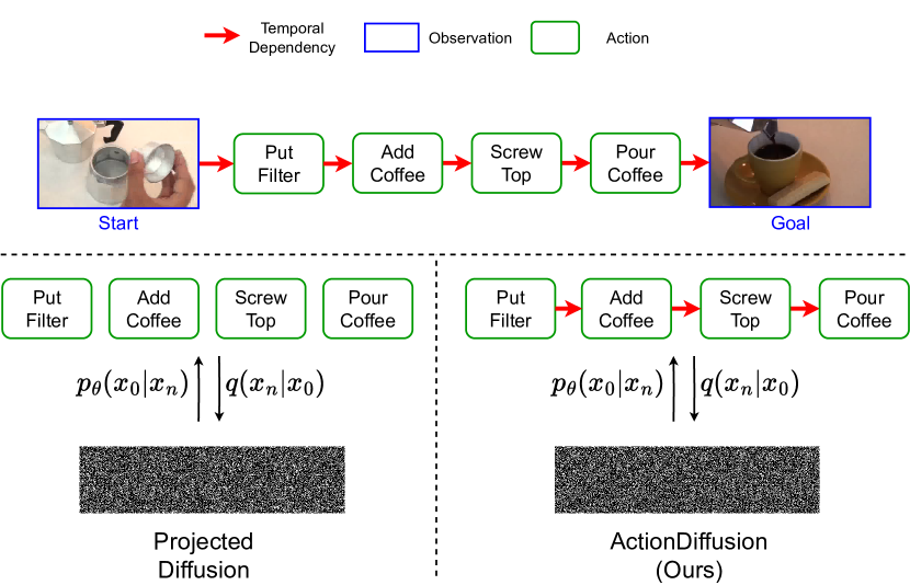
Figure 1: Procedure planning in instructional videos using diffusion models. Previous work (Projected Diffusion) [14] does not take the temporal dependencies between actions into account. Our method (ActionDiffusion) incorporates these dependencies directly into the diffusion model.

Diffusion models [15] have achieved outstanding results in many research fields such as in image generation [15, 16], text-to-image generation [17, 18, 19], trajectory planning [20, 21], video generation [22, 23], human motion prediction [24], of time series imputation [25]. The current state-of-the-art method for procedure planning in videos [14] is also based on a diffusion model. Unlike diffusion models for images, the input for diffusion-based procedure planning is a multi-dimensional matrix that consists of the visual observations of the start and goal, the sequence of actions, and task classes. At inference time, the input matrix is reconstructed and the dimension containing the action sequence is the prediction of the action plan. A key limitation of this method is that the influence of the temporal dependencies between actions, i.e. that actions are more likely to cause particular follow-up actions, has not been considered. Although the input matrix in [14] contains the action labels during training, the diffusion model still treats the input matrix as a static “image”, it does not learn its inherent temporal dependencies.

To overcome this limitation we propose Action-aware Noise Mask Diffusion (ActionDiffusion) – the first method that leverages the temporal dependencies between actions into the diffusion process (see Figure 1). Our method learns the temporal dependencies of actions in the noise space of the diffusion instead of the feature space, thereby unifying the tasks of learning temporal dependencies and generating action plans in the diffusion steps. More specifically, we first propose an action-aware noise mask for the noise-adding stage of the diffusion model. We add the action embeddings in addition to the Gaussian noise in the noise masks so that the model input is transformed into Gaussian noises by iteratively adding the action-aware noise. Second, we introduce an attention mechanism in the denoising neural network (U-Net) to learn the correlations between actions. During the inference, it then can predict action-aware noises to generate action plans. In line with previous work [13, 14], we evaluate the performance of ActionDiffusion through experiments on three popular instructional video benchmarks: CrossTask [9], Coin [10], and NIV [11] with various time horizons. Our results show that ActionDiffusion achieves State-Of-The-Art (SOTA) performances across different metrics for all time horizons on all three datasets. We demonstrate that by adding action embeddings into the noise mask, the diffusion model can effectively learn the temporal dependencies between actions and increase the performance on procedure planning in instructional videos.

The specific contributions of our work are threefold: 1) We propose ActionDiffusion, a novel method incorporating the action temporal dependencies in the diffusion model for procedure planning in instructional videos. We unify the learning of temporal dependencies and action plan generation in the noise space. 2) We add action embeddings into noise masks in the noising-adding stage of diffusion models and use a denoising neural network with self-attention to better learn and predict the action-aware noise to reconstruct the action plan in the denoising phase. 3) We evaluate our methods on CrossTask, Coin, and NIV datasets across various time horizons and achieve SOTA performances in multiple metrics and show the advantage of incorporating action temporal dependencies in the diffusion model, which previous work did not consider.

II Method

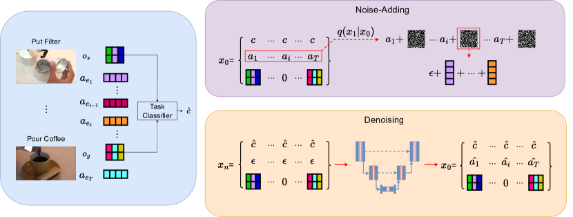
Figure 2: Overview of ActionDiffusion. From an instructional video, we extract the visual feature of the start state $o_{s}$ and the goal state $o_{g}$ as well as the features of actions $a_{e_{1:T}}$. We use the task class $c$, one-hot action class $a_{1:T}$, $o_{s}$ and $o_{g}$ as the input of the diffusion model. Note that in the training, we use the ground truth task class $c$ and predicted task class $\hat{c}$ during inference. A separate task classifier is trained to get $\hat{c}$. In the noise-adding phase in training, the noise is added on $a_{1:T}$. For each action, we add all previous action embeddings and the current action embedding in addition to the Gaussian noise. In the denoising phase during inference, we use the U-Net with attention to predict the action-aware noise to denoise $x_{n}$. The predicted action plan is the action sequence $\hat{a}_{1:T}$ from the reconstructed input $x_{0}$.

II-A Problem Formulation

We adopt the problem formulation of procedure planning used in previous work [2, 14]: Given the visual observation of the start state $o_{s}$ and the goal state $o_{g}$, the task is to predict the intermediate steps, i.e., the action plan $\pi=a_{1:T}$ for a chosen time horizon $T$. The action plan $\pi$ will transform $o_{s}$ to $o_{g}$. More formally, this task can be written as,

$$p(\pi\mid o_{s},o_{g})=\int p(\pi\mid o_{s},o_{g},\hat{c})\;p(\hat{c}\mid o_{s},o_{g})\,d\hat{c},$$ (1)

where $\hat{c}$ is the predicted task class of the video (e.g., cooking a specific meal). The planning is decomposed into two steps [14]: 1) predicting the task class $\hat{c}$ given the start state $o_{s}$ and the goal state $o_{g}$, 2) inferring the action plan $\pi$ given $o_{s}$, $o_{g}$, and $\hat{c}$ by sampling from the diffusion model.

II-B Action-aware Noise Mask Diffusion

Figure 2 provides an overview of our proposed ActionDiffusion method. Taking an instructional video as input, the method first extracts the visual features of the start state $o_{s}$, the goal state $o_{g}$, and of action embeddings $a_{e_{1:T}}$. It then uses the task class $c$, one-hot action class $a_{1:T}$, $o_{s}$, and $o_{g}$ to form the input for the diffusion model. Note that during training, we use the ground truth task class $c$ while the predicted task class $\hat{c}$ is used during inference. To obtain $\hat{c}$ we train a separate task classifier that models $p(\hat{c}\mid o_{s},o_{g})$ in Equation (1). In the noise-adding phase, during training, the noise is added on $a_{1:T}$ in the model input $x_{0}$. For each action, we add all previous as well as the current action embedding in addition to the Gaussian noise. In the denoising phase, during inference, we use a U-Net with attention to predict the action-aware noise to denoise the noisy input $x_{n}$ at step $n$. The action sequence $\hat{a}_{1:T}$ from the reconstructed input $x_{0}$ is the predicted action plan (see below for details).

II-C Diffusion Model

A diffusion model [15] takes input $x_{0}$ and performs two steps on the input: The first one is the noise-adding step, where Gaussian noise $\epsilon\sim\mathcal{N}(0,\mathbf{I})$ is added to $x_{0}$ incrementally and eventually $x_{0}$ approaches a standard Gaussian distribution in $x_{N}$. This noise-adding process $q(x_{n}\mid x_{n-1})$ for $n=N,\ldots,1$ is described by the following equation,

$$q(x_{n}\mid x_{n-1})=\mathcal{N}(x_{n};\sqrt{1-\beta_{n}}x_{n-1},\beta_{n}\mathbf{I}),$$ (2)

where $\beta_{n}\in(0,1)$ is pre-defined (see below). $\beta_{n}$ decides how much of the noise is added to $x_{n}$. A re-parameterization is then applied,

$$x_{n}=\sqrt{\bar{\alpha}_{n}}x_{0}+\sqrt{1-\bar{\alpha}_{n}}\epsilon,$$ (3)

where $\bar{\alpha}_{n}=\prod_{s=1}^{n}(1-\beta_{s})$. A cosine noise scheduling technique [16] is used to determine $\{\beta_{s}\}_{s=1}^{n}$,

$$\bar{\alpha}_{n}=\frac{f(n)}{f(0)},\\ f(n)=\text{cos}(\frac{n/N+\tau}{1+\tau}\times\frac{\pi}{2})^{2},$$ (4)

where $\tau$ is an offset value to prevent $\beta_{n}$ from becoming too small when $n$ is close to 0.

The second step is the denoising process, where the diffusion model samples $x_{N}$ from Gaussian noise $\mathcal{N}(0,\mathbf{I})$ and denoises $x_{N}$ to obtain $x_{0}$ via the denoising process

$$p_{\theta}(x_{n-1}\mid x_{n})=\mathcal{N}(x_{n-1};\mu_{\theta}(x_{n},n),\Sigma_{\theta}(x_{n},n)),$$ (5)

where $\mu_{\theta}(x_{n},n)$ is parameterised by a neural network $\epsilon_{\theta}(x_{n},n)$, and $\Sigma_{\theta}(x_{n},n)$ is calculated by using $\beta_{n}\mathbf{I}$.

II-D Action-aware Noise Mask

We follow [14] to construct the input $x_{0}$ to the diffusion model as,

$$x_{0}=\begin{bmatrix}c&c&...&c&c\\ a_{1}&a_{2}&...&a_{T-1}&a_{T}\\ o_{s}&0&...&0&o_{g}\end{bmatrix},$$ (6)

at the noise-adding step, the noise is only added to the action dimension, i.e. $a_{1:T}$ and $a_{i}$ is a one-hot vector of a number of $A$ action classes, thus $\mathbf{I}\in\mathbb{R}^{T\times A}$ in Equation (2). We design an action-aware noise mask $M_{a}$ with multiple previous actions accumulated (multi-add) as

$$M_{a}=\begin{bmatrix}0&0&...&0\\ g(a_{e_{1}})&\sum_{i=1}^{2}g(a_{e_{i}})&...&\sum_{i=1}^{T}g(a_{e_{i}})\\ 0&0&...&0\end{bmatrix},$$ (7)

where $a_{e_{1:T}}$ are the embeddings of $a_{1:T}$, and $g(\cdot)$ normalises the embeddings to the range of [-1, 1]. Essentially, in addition to the Gaussian noise applied to $x_{0}$, we add the normalised action embeddings to the noise mask. In the temporal direction, we accumulate all previous action embeddings. Our intuition is that at each $i\in[2:T]$ the noise mask knows what the previous actions are and $\epsilon_{\theta}$ can learn the temporal dependencies of actions in the denoising stage. With the action-aware noise mask, Equation (2) then becomes,

$$q(x_{n}\mid x_{n-1})=\mathcal{N}(x_{n};\sqrt{1-\beta_{n}}x_{n-1},\beta_{n}(\mathbf{I}+M_{a})),$$ (8)

we again apply re-parameterisation and update Equation (3),

$$x_{n}=\sqrt{\bar{\alpha}_{n}}x_{0}+\sqrt{1-\bar{\alpha}_{n}}\epsilon_{a}.$$ (9)

II-E Denoising Neural Network

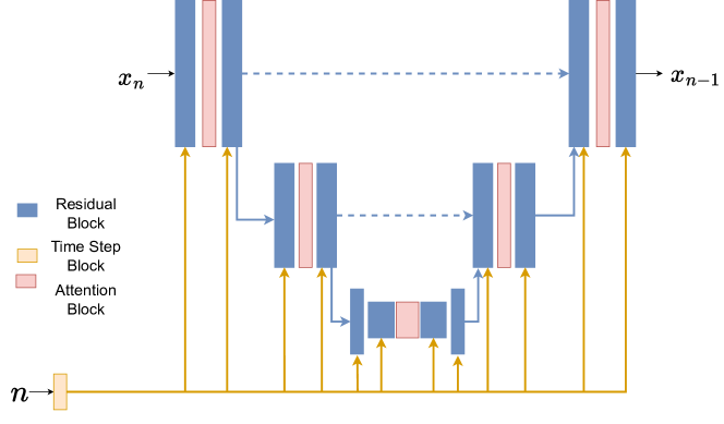
Figure 3: Architecture of the noise prediction neural network $\epsilon_{\theta}$. The network $\epsilon_{\theta}$ is based on U-Net and incorporates attention mechanisms.

Following [14], we use a U-Net as the noise prediction neural network $\epsilon_{\theta}$. To better learn the temporal dependencies between actions we further propose to incorporate an attention mechanism [26, 17]. Figure 3 shows the architecture of the U-Net with attention. As indicated in Equation (5), the U-Net takes $x_{n}$ and noise schedule time step $n$ as input. $n$ is first passed to a time step block and then is fed to all residual blocks. The attention block enables self-attention [27].

II-F Training

In the training phase, the input $x_{0}$ to the diffusion model uses ground truth task class $c$. However, during the inference phase, we need the predicted task class $\hat{c}$ since the procedure planning task has only access to $o_{s}$ and $o_{g}$ to infer $\pi$. Thus, we train an MLP for predicting $\hat{c}$ using $c$ as supervision. Next, we train the diffusion model using the following squared loss function,

$$\mathcal{L}=\sum_{n=1}^{N}(\epsilon_{\theta}(x_{n},n),x_{0})^{2}.$$ (10)

II-G Inference

During inference, only $o_{s}$ and $o_{g}$ are given and we need to sample the action plan $\pi$. We start with constructing $x_{n}$. Then, the noise prediction neural network $\epsilon_{\theta}$ predicts the noise iteratively to denoise $x_{n}$ into $x_{0}$. Here, $x_{n}$ is

$$x_{n}=\begin{bmatrix}\hat{c}&\hat{c}&...&\hat{c}&\hat{c}\\ \epsilon&\epsilon&...&\epsilon&\epsilon\\ o_{s}&0&...&0&o_{g}\end{bmatrix},$$ (11)

only the action plan is initialised with Gaussian noise and $\epsilon\in\mathcal{N}(0,\mathbf{I})$ since the noise is only added to the actions during the noise-adding stage. Although we use action-aware noise masks in the noise-adding stage, we do not need to encode action information into the Gaussian noise. The reason is that, after adding noise to $x_{0}$ with $N$ steps, $x_{N}$ already approximates Gaussian noise by construction. After $N$ steps of denoising, we take the action sequence $\hat{a}_{1:T}$ as the action plan $\pi$.

III Experiments

III-A Datasets

We evaluate ActionDiffusion on three instructional video benchmark datasets: CrossTask [9], Coin [10], and NIV [11]. The CrossTask dataset contains 2,750 videos, 18 tasks, and 105 action classes. The average number of actions per video is 7.6. The Coin dataset has a much larger number of videos, tasks, and action classes: In total, it contains 11,827 videos, 180 tasks, and 778 action classes. The average number of actions per video is 3.6. Finally, the NIV dataset is the smallest among the three datasets. It contains 150 videos, five tasks, and 18 action classes as well as 9.5 actions per video on average. We follow the data curation process used in previous work [2, 14]: For a video containing $m$ number of actions, we extract action sequences with the time horizon $T$ using a sliding window. For an extracted action sequence $[a_{i},...,a_{i+T-1}]$, each action has a corresponding video clip. We extract the video clip feature at the beginning of $a_{i}$ as the visual observation of the start state $o_{s}$ and the video clip feature at the end of $a_{i+T-1}$ as the goal state $o_{g}$. To facilitate comparability, we use the pre-extracted features from previous work [13, 14]. The features were extracted by using a model [28] which was pre-trained on the HowTo100M dataset [29]. In addition to the video clip features, the model also generated embeddings for actions corresponding to video clips. We use the action embeddings for our action-aware diffusion. We randomly use 70% of the data for training and 30% for testing.

III-B Metrics

We use three metrics for evaluation: The first metric is the Success Rate (SR). An action plan is considered correct, and thus the procedure planning is a success, only if all actions in the plan are correct and the order of the actions is correct. This is the most strict metric. The second metric is the mean Accuracy (mAcc). The accuracy is calculated based on the individual actions in the action plan. The order of the actions is not considered. The last metric is mean Single Intersection over Union (mSIoU). The calculation of IoU treats the predicted action plans and the ground truth action plans as sets and also does not consider the order of actions. The works in [2, 13, 12] calculated mIoU with all action plans in a mini-batch. However, as pointed out in [14], this calculation is dependent on the batch size. To ensure a fairer comparison, they proposed the mSIoU metric instead, which treats each single action plan as a set and is thus agnostic to the batch size. We also opted for the mSIoU metric.

III-C Baselines

We compare our method with several state-of-the-art baseline methods for procedure planning:

• DDN [2] uses MLPs and RNNs to learn the dynamics between actions and observations and uses search algorithms to sample the action plan.

• Ext-GAIL [12] models action sequence as a Markov Decision Process (MDP) and uses imitation learning to learn policies to sample actions.

• P³IV [13] uses transformers with a memory block and a generative module trained with adversarial loss was used to sample the action plan.

• PDPP [14] uses a diffusion model to generate the action plan with the task class, start observation, and goal observation as conditions.

IV Results

IV-A Comparison to SOTA Methods

IV-A1 CrossTask

TABLE I: Results on Crosstask dataset with time horizon $T=3$ and $T=4$. Numbers in Bold indicate the best results. The arrow ↑ means higher numbers are better.

	T=3			T=4
	SR(%)↑	mAcc(%)↑	mSIoU(%)↑	SR(%)↑	mAcc(%)↑	mSIoU(%)↑
DDN [2]	12.18	31.29	-	5.97	27.10	-
Ext-GAIL [12]	21.27	49.46	-	16.41	43.05	-
P3IV [13]	23.34	49.96	-	13.40	44.16	-
PDPP [14]	37.20	64.67	66.57	21.48	57.82	65.13
ActionDiffusion-Multi-Add (Ours)	37.86	65.58	67.54	22.28	59.30	65.80

Table I shows the results on the CrossTask dataset with time horizon $T=3$ and $T=4$. ActionDiffusion achieves SOTA performances for all metrics in both time horizons. Note that DNN, Ext-GAIL, and P³IV only reported mIoU, and only PDPP reported mSIoU. We also evaluate our method with the longer time horizon $T\in\{3,4,5,6\}$. Table II shows the SR for all the time horizons. We again have SOTA performances in all time horizons.

TABLE II: Results on Crosstask dataset with time horizon $T\in\{3,4,5,6\}$. Numbers in Bold indicate the best results. The arrow ↑ means higher numbers are better.

	T=3	T=4	T=5	T=6
	SR(%)↑	SR(%)↑	SR(%)↑	SR(%)↑
DDN [2]	12.18	5,97	3.10	1.20
Ext-GAIL [12]	21.27	16.41	-	-
P3IV [13]	23.34	13.40	7.21	4.40
PDPP [14]	37.20	21.48	13.45	8.41
ActionDiffusion-Multi-Add (Ours)	37.86	22.28	13.93	9.13

IV-A2 Coin

TABLE III: Results on Coin and NIV datasets with time horizon $T=3$ and $T=4$. Numbers in Bold indicate the best results. The arrow ↑ means higher numbers are better. ActionDiffusion means our method using Multi-Add mask.

		COIN			NIV
Horizon	Models	SR(%)↑	mAcc(%)↑	mSIoU(%)↑	SR(%)↑	mAcc(%)↑	mSIoU(%)↑
T=3	DDN	13.90	20.19	-	18.41	32.54	-
	Ext-GAIL	-	-	-	22.11	42.20	-
	P3IV	15.40	21.67	-	24.68	49.01	-
	PDPP	21.33	45.62	51.82	30.20	48.45	57.28
	ActionDiffusion-Multi (Ours)	23.58	45.24	53.86	32.96	49.01	57.85
T=4	DDN	11.13	17.71	-	15.97	2.73	-
	Ext-GAIL	-	-	-	19.91	36.31	-
	P3IV	11.32	18.85	-	20.14	28.36	-
	PDPP	14.41	44.10	51.39	26.67	46.89	59.45
	ActionDiffusion-Multi (Ours)	17.98	44.43	56.00	29.26	47.71	60.90

Table III shows the results on the Coin dataset with time horizon $T=3$ and $T=4$. For $T=3$, we achieved SOTA performance on SR and mSIOU. Although the mAcc is slightly lower than PDPP, our SR is still 2.25% higher than PDPP. This means that ActionDiffusion can learn the temporal dependencies better than PDPP even though the percentage of correctly predicted actions (ignoring the order) is slightly lower. When $T=4$, we have SOTA results on all metrics. Our mAcc is slightly better than PDPP, SR and mSIoU are 3.57% and 4.61% higher. This also shows our method is better at capturing the temporal dependencies.

IV-A3 NIV

The results on the NIV dataset are shown in Table III. We obtain SOTA performance on all metrics in both time horizons. The SR is 2.76% higher than PDPP when $T=3$ and 2.59% higher when $T=4$.

IV-B Ablation Study

IV-B1 Multi-Add Mask VS. Single-Add Mask

In Equation (7), we describe the Multi-Add action-aware noise mask. At each time step within the time horizon $T$, we accumulate the embeddings of all previous actions. We want to compare it with Single-Add noise mask described as follows,

$$\begin{bmatrix}0&0&...&0\\ g(a_{e_{1}})&g(a_{e_{1}})+g(a_{e_{2}})&...&g(a_{e_{T-1}})+g(a_{e_{T}})\\ 0&0&...&0\end{bmatrix},$$ (12)

where at each time step only the previous action embedding is added to the noise mask. Table IV shows the results of the Multi-Add mask and Single-Add mask on all three datasets with time horizon $T=3$ and $T=4$. Multi-Add outperforms Single-Add on all metrics on the Coin dataset and NIV dataset. On the CrossTask dataset, Single-Add only performs slightly better on SR, and Multi-Add is still better on mAcc and mSIoU. Overall, Multi-Add can better capture and preserve the temporal dependencies between actions.

TABLE IV: Comparison between multi-add noise mask and single-add noise mask on Crosstask, Coin and NIV datasets. Numbers in Bold indicate the best results. The arrow ↑ means higher numbers are better.

		T=3			T=4
Dataset	Models	SR↑	mAcc↑	mSIoU↑	SR↑	mAcc↑	mSIoU↑
Crosstask	ActionDiffusion-Multi	37.86	65.58	67.54	22.28	59.30	65.80
	ActionDiffusion-Single	38.21	65.34	67.25	22.32	58.92	65.26
Coin	ActionDiffusion-Multi	23.58	45.24	53.86	17.98	44.43	56.00
	ActionDiffusion-Single	21.52	43.13	52.98	14.97	42.56	55.04
NIV	ActionDiffusion-Multi	32.96	49.01	57.85	29.26	47.71	60.90
	ActionDiffusion-Single	30.74	47.03	56.00	25.76	44.98	57.92

IV-B2 Self-Attention in U-Net

TABLE V: Comparison between the U-Net with self-attention (w attention) and the U-Net without self-attention (w/o attention). Numbers in Bold indicate the best results. The arrow ↑ means higher numbers are better.

		T=3			T=4
Dataset	Models	SR↑	mAcc↑	mSIoU↑	SR↑	mAcc↑	mSIoU↑
Crosstask	w attention	37.86	65.58	67.54	22.28	59.30	65.80
	w/o attention	37.86	65.54	67.57	22.38	59.18	65.99
Coin	w attention	23.58	45.24	53.86	17.98	44.43	56.00
	w/o attention	23.14	44.80	54.00	18.06	44.83	56.32
NIV	w attention	32.96	49.01	57.85	29.26	47.71	60.90
	w/o attention	31.85	46.30	56.37	27.95	46.52	58.55

We study the effect of the self-attention mechanism in the U-Net in this section. We use the Multi-Add noise mask and test the U-Net with and without self-attention on all three datasets. The results are shown in Table V. ActionDiffusion with and without self-attention achieve comparable results on the CrossTask dataset. On the Coin dataset, ActionDiffusion with and without self-attention also have comparable results. ActionDiffusion with self-attention performs better on SR and mACC when $T=3$. On the NIV dataset, ActionDiffusion with self-attention outperforms the one without self-attention on all metrics with both time horizons. Overall, ActionDiffusion with self-attention performs better than without self-attention on the NIV dataset, while they have comparable performance on the other two datasets. We interpret the reason for this as the size of NIV is much smaller than the other two. ActionDiffusion with attention can better learn the temporal dependencies integrated into the noise mask when the data is limited.

V Conclusion

In this work, we propose ActionDiffusion, an action-aware diffusion model, to tackle the challenge of procedure planning in instructional videos. We integrate temporal dependencies between actions by adding action embeddings to the noise mask during the diffusion process. We achieve SOTA performances on three procedure planning datasets across multiple metrics, showing the novelty of adding action embedding in the noise mask as the modelling of temporal dependencies.

References

- [1] M. Lippi, P. Poklukar, M. C. Welle, A. Varava, H. Yin, A. Marino, and D. Kragic, “Latent space roadmap for visual action planning of deformable and rigid object manipulation,” in 2020 IEEE/RSJ International Conference on Intelligent Robots and Systems (IROS). IEEE, 2020, pp. 5619–5626.
- [2] C.-Y. Chang, D.-A. Huang, D. Xu, E. Adeli, L. Fei-Fei, and J. C. Niebles, “Procedure planning in instructional videos,” in European Conference on Computer Vision. Springer, 2020, pp. 334–350.
- [3] Y. Han, W. Hao, and U. Vaidya, “Deep learning of koopman representation for control,” in 2020 59th IEEE Conference on Decision and Control (CDC). IEEE, 2020, pp. 1890–1895.
- [4] B. van der Heijden, L. Ferranti, J. Kober, and R. Babuška, “Deepkoco: Efficient latent planning with a task-relevant koopman representation,” in 2021 IEEE/RSJ International Conference on Intelligent Robots and Systems (IROS). IEEE, 2021, pp. 183–189.
- [5] D. Hafner, T. Lillicrap, I. Fischer, R. Villegas, D. Ha, H. Lee, and J. Davidson, “Learning latent dynamics for planning from pixels,” in International conference on machine learning. PMLR, 2019, pp. 2555–2565.
- [6] K. Fang, Y. Zhu, A. Garg, S. Savarese, and L. Fei-Fei, “Dynamics learning with cascaded variational inference for multi-step manipulation,” arXiv preprint arXiv:1910.13395, 2019.
- [7] J. Sun, D.-A. Huang, B. Lu, Y.-H. Liu, B. Zhou, and A. Garg, “Plate: Visually-grounded planning with transformers in procedural tasks,” IEEE Robotics and Automation Letters, vol. 7, no. 2, pp. 4924–4930, 2022.
- [8] N. Kumar, W. McClinton, R. Chitnis, T. Silver, T. Lozano-Pérez, and L. P. Kaelbling, “Learning efficient abstract planning models that choose what to predict,” in Conference on Robot Learning. PMLR, 2023, pp. 2070–2095.
- [9] D. Zhukov, J.-B. Alayrac, R. G. Cinbis, D. Fouhey, I. Laptev, and J. Sivic, “Cross-task weakly supervised learning from instructional videos,” in Proceedings of the IEEE/CVF Conference on Computer Vision and Pattern Recognition, 2019, pp. 3537–3545.
- [10] Y. Tang, D. Ding, Y. Rao, Y. Zheng, D. Zhang, L. Zhao, J. Lu, and J. Zhou, “Coin: A large-scale dataset for comprehensive instructional video analysis,” in Proceedings of the IEEE/CVF Conference on Computer Vision and Pattern Recognition, 2019, pp. 1207–1216.
- [11] J.-B. Alayrac, P. Bojanowski, N. Agrawal, J. Sivic, I. Laptev, and S. Lacoste-Julien, “Unsupervised learning from narrated instruction videos,” in Proceedings of the IEEE Conference on Computer Vision and Pattern Recognition, 2016, pp. 4575–4583.
- [12] J. Bi, J. Luo, and C. Xu, “Procedure planning in instructional videos via contextual modeling and model-based policy learning,” in Proceedings of the IEEE/CVF International Conference on Computer Vision, 2021, pp. 15 611–15 620.
- [13] H. Zhao, I. Hadji, N. Dvornik, K. G. Derpanis, R. P. Wildes, and A. D. Jepson, “P3iv: Probabilistic procedure planning from instructional videos with weak supervision,” in Proceedings of the IEEE/CVF Conference on Computer Vision and Pattern Recognition, 2022, pp. 2938–2948.
- [14] H. Wang, Y. Wu, S. Guo, and L. Wang, “Pdpp: Projected diffusion for procedure planning in instructional videos,” in Proceedings of the IEEE/CVF Conference on Computer Vision and Pattern Recognition, 2023, pp. 14 836–14 845.
- [15] J. Ho, A. Jain, and P. Abbeel, “Denoising diffusion probabilistic models,” Advances in neural information processing systems, vol. 33, pp. 6840–6851, 2020.
- [16] A. Q. Nichol and P. Dhariwal, “Improved denoising diffusion probabilistic models,” in International Conference on Machine Learning. PMLR, 2021, pp. 8162–8171.
- [17] R. Rombach, A. Blattmann, D. Lorenz, P. Esser, and B. Ommer, “High-resolution image synthesis with latent diffusion models,” in Proceedings of the IEEE/CVF conference on computer vision and pattern recognition, 2022, pp. 10 684–10 695.
- [18] L. Zhang, A. Rao, and M. Agrawala, “Adding conditional control to text-to-image diffusion models,” in Proceedings of the IEEE/CVF International Conference on Computer Vision, 2023, pp. 3836–3847.
- [19] N. Ruiz, Y. Li, V. Jampani, Y. Pritch, M. Rubinstein, and K. Aberman, “Dreambooth: Fine tuning text-to-image diffusion models for subject-driven generation,” in Proceedings of the IEEE/CVF Conference on Computer Vision and Pattern Recognition, 2023, pp. 22 500–22 510.
- [20] M. Janner, Y. Du, J. B. Tenenbaum, and S. Levine, “Planning with diffusion for flexible behavior synthesis,” arXiv preprint arXiv:2205.09991, 2022.
- [21] S. Huang, Z. Wang, P. Li, B. Jia, T. Liu, Y. Zhu, W. Liang, and S.-C. Zhu, “Diffusion-based generation, optimization, and planning in 3d scenes,” in Proceedings of the IEEE/CVF Conference on Computer Vision and Pattern Recognition, 2023, pp. 16 750–16 761.
- [22] J. Ho, W. Chan, C. Saharia, J. Whang, R. Gao, A. Gritsenko, D. P. Kingma, B. Poole, M. Norouzi, D. J. Fleet, et al., “Imagen video: High definition video generation with diffusion models,” arXiv preprint arXiv:2210.02303, 2022.
- [23] Z. Luo, D. Chen, Y. Zhang, Y. Huang, L. Wang, Y. Shen, D. Zhao, J. Zhou, and T. Tan, “Videofusion: Decomposed diffusion models for high-quality video generation,” in Proceedings of the IEEE/CVF Conference on Computer Vision and Pattern Recognition, 2023, pp. 10 209–10 218.
- [24] H. Yan, Z. Hu, S. Schmitt, and A. Bulling, “Gazemodiff: Gaze-guided diffusion model for stochastic human motion prediction,” arXiv preprint arXiv:2312.12090, 2023.
- [25] Y. Tashiro, J. Song, Y. Song, and S. Ermon, “Csdi: Conditional score-based diffusion models for probabilistic time series imputation,” Advances in Neural Information Processing Systems, vol. 34, pp. 24 804–24 816, 2021.
- [26] P. Dhariwal and A. Nichol, “Diffusion models beat gans on image synthesis,” Advances in neural information processing systems, vol. 34, pp. 8780–8794, 2021.
- [27] A. Vaswani, N. Shazeer, N. Parmar, J. Uszkoreit, L. Jones, A. N. Gomez, Ł. Kaiser, and I. Polosukhin, “Attention is all you need,” Advances in neural information processing systems, vol. 30, 2017.
- [28] A. Miech, J.-B. Alayrac, L. Smaira, I. Laptev, J. Sivic, and A. Zisserman, “End-to-end learning of visual representations from uncurated instructional videos,” in Proceedings of the IEEE/CVF Conference on Computer Vision and Pattern Recognition, 2020, pp. 9879–9889.
- [29] A. Miech, D. Zhukov, J.-B. Alayrac, M. Tapaswi, I. Laptev, and J. Sivic, “Howto100m: Learning a text-video embedding by watching hundred million narrated video clips,” in Proceedings of the IEEE/CVF international conference on computer vision, 2019, pp. 2630–2640.