Machine Learning Optimized Orthogonal Basis Piecewise Polynomial Approximation

Abstract

Piecewise Polynomials (PPs) are utilized in several engineering disciplines, like trajectory planning, to approximate position profiles given in the form of a set of points. While the approximation target along with domain-specific requirements, like $\mathcal{C}^{k}$-continuity, can be formulated as a system of equations and a result can be computed directly, such closed-form solutions posses limited flexibility with respect to polynomial degrees, polynomial bases or adding further domain-specific requirements. Sufficiently complex optimization goals soon call for the use of numerical methods, like gradient descent. Since gradient descent lies at the heart of training Artificial Neural Networks (ANNs), modern Machine Learning (ML) frameworks like TensorFlow come with a set of gradient-based optimizers potentially suitable for a wide range of optimization problems beyond the training task for ANNs. Our approach is to utilize the versatility of PP models and combine it with the potential of modern ML optimizers for the use in function approximation in 1D trajectory planning in the context of electronic cam design. We utilize available optimizers of the ML framework TensorFlow directly, outside of the scope of ANNs, to optimize model parameters of our PP model. In this paper, we show how an orthogonal polynomial basis contributes to improving approximation and continuity optimization performance. Utilizing Chebyshev polynomials of the first kind, we develop a novel regularization approach enabling clearly improved convergence behavior. We show that, using this regularization approach, Chebyshev basis performs better than power basis for all relevant optimizers in the combined approximation and continuity optimization setting and demonstrate usability of the presented approach within the electronic cam domain.

1 Introduction

1.1 Motivation

PPs are of special interest in several science and engineering disciplines, where the latter are particularly interesting, as they come with additional physical constraints. Path and trajectory planning for machines in the field of mechatronics are just two examples. Path planning is the task of finding possible waypoints of a robot or automated machine to move through its environment without collision. Trajectory planning computes time-dependent positional, velocity or acceleration profiles that hold setpoints for controllers of robots or automated machines to move joints from one waypoint to the other. Electronic cams are a subfield of the latter, describing repetitive motion executed by servo drives within industrial machines. In this context, positional, velocity or acceleration profiles are defined as input point clouds and approximated by PPs, which are then processed by industrial servo drives, like B&R Industrial Automation’s ACOPOS series. Conventionally, the approximation target along with domain-specific requirements such as continuity, cyclicity or periodicity are formulated as a system of equations and a closed-form solution is computed. While computational effort may be low for computing such closed-form solutions, they posses limited flexibility with respect to polynomial degrees, polynomial bases or adding further domain-specific requirements. Sufficiently complex optimization goals soon call for the use of numerical methods, like gradient descent.

Training an ANN is the iterative process of adapting weights of node connections in order to fit given training data. With the advent of ML frameworks, this iterative training task is commonly carried out by calculating gradients using automatic differentiation and updating weights according to the gradient descent algorithm. Since gradient descent lies at the heart of this process, modern ML frameworks like TensorFlow or PyTorch therefore come with a set of gradient-based optimizers potentially suitable for a wide range of optimization problems beyond the training task for ANNs. Since advances in deep learning rely on these optimizers, state-of-the art insights within the field are continuously implemented, holding the potential of better performance than classical gradient descent optimizers.

Our approach therefore is to utilize the versatility of PP models and combine it with the potential of modern ML optimizers for the use in function approximation in 1D trajectory planning in the context of electronic cam design. We utilize available optimizers of the ML framework TensorFlow directly, outside of the scope of ANNs, to optimize model parameters of our PP model. This allows for an optimization of trajectories with respect to dynamic criteria using state of the art methods, while at the same time working with an explainable model, allowing to directly derive physical properties like velocity, acceleration or jerk. Although our work documented in [6] shows that our approach is basically feasible, experiments show that clean convergence especially regarding continuity optimization requires further practical considerations and regularization techniques. In an attempt to overcome these shortcomings, in this paper, we show how an orthogonal polynomial basis contributes to significantly improving approximation and continuity optimization performance.

1.2 An Orthogonal Basis

Orthogonal polynomial sets are beneficial for determining the best polynomial approximation to an arbitrary function $f$ in the least squares sense, resulting from the fact that every polynomial in such an orthogonal system possesses a minimal $L_{2}$ property with respect to the system’s weight function, see [8] for details. Among different sets of orthogonal polynomials, Chebyshev polynomials of the first kind are of special interest. Besides favorable numerical properties, like the absolute values such polynomials evaluate to staying within the unit interval, their roots are well known as nodes (Chebyshev nodes) in polynomial interpolation to minimize the problem of Runge’s phenomenon. This effect is interesting for us, as we are anticipating reduced oscillating behavior beneficial for our electronic cam approximation setting. Additionally and contrary to Chebyshev polynomials of the second kind, numerous efficient algorithms exist for the conversion between orthogonal basis and power basis representations [2]. (We need this in the end, since our solution targets servo drives like B&R Industrial Automation’s ACOPOS series processing cam profiles as a power basis PP function.) With respect to potential future work, the relationship of Chebyshev series to Fourier cosine series has the potential of allowing a more straightforward formal approach to spectral analysis and optimization of generated cam profiles (e.g. to reduce resonance vibrations), since it inherits theorems and properties of Fourier series, allowing for a Chebyshev transform analogue to Fourier transform [4]. These arguments make Chebyshev polynomials of the first kind an attractive subject of investigation for this paper.

1.3 Related work

There is a lot of published work on approximation using PP in the cam approximation domain that rely on a closed-form expression in order to non-iteratively calculate a solution, like [9]. Although computational effort is reduced using such approaches, as mentioned earlier, they posses limited flexibility with respect to polynomial degrees, bases and complexity of loss functions. There also is work on PP approximation using “classical” gradient based approaches. In [3], Voronoi tessellation is used for partitioning the input space before approximating given 2D surfaces using a gradient-based approach with multivariate PPs. The authors state that an orthogonal basis is beneficial for this task, however, develop their approach using power basis. Contrary to our work, the loss function only comprises the approximation error, which implies that continuity is not achieved by their approach. Furthermore, the authors state that magnitudes of derivatives of the error function may vary greatly, thus making classical gradient descent approaches unusable. We show in this paper, that regularization may mitigate this effect, at least for continuity optimization in the 1D setting.

Other work utilizes parametric functions for approximation of given input data, like B-Spline or NURBS curves, as in [10]. This has some benefits over non-parametric PPs: For one, $\mathcal{C}^{k}$-continuity is given simply by the choice of order of the curve. For another, fewer parameters (usually control points) need to be optimized. However, PP models are utilized in several engineering disciplines and conversion from parametric curves is not generally possible. As an example, servo drives, like B&R Industrial Automation’s ACOPOS series, process electronic cams in a PP format.

ANNs are investigated for the use in function approximation. In [1], the authors provide an overview of the state-of-the art with respect to aspects like numerical stability or accuracy and develop a computational framework for examining the performance of ANNs in this respect. Although results look promising and other recent works, like [11], already provide algorithmic bounds for the ANN approximation setting, one of the main drivers for the use of a PP model outside of the context of neural networks for our work is explainability. When utilizing Artificial Intelligence (AI) methods in the domain of electronic cams, there is a strong necessity for explainability, mainly rooted in the fact that movement of motors and connected kinematic chains like robotic arms affects its physical environment with the potential of causing harm, therefore calling for predictable movement. This, in turn, calls for a “predictable model”, that allows to reliably derive physical properties and generate statements about expected behavior. Another recent development tackling these challenges are Physics-informed Neural Networks (PINNs), where resulting ANNs can be described using partial differential equations. For the domain of 1D electronic cam approximation covered in this work, however, using PP models is simpler and more intuitive considering that servo drives directly utilize PPs.

There are some preliminary non-scientific texts (e.g. personal blog articles) on gradient descent optimization for polynomial regression utilizing ML optimizers for a single polynomial segment. However, to the best of our knowledge, there is no published work on utilizing gradient descent optimizers of modern ML frameworks for $\mathcal{C}^{k}$-continuous PP approximation other than our previous research published in [6].

1.4 Contributions

Although Chebyshev basis holds the potential of improved approximation optimization performance, our experiments show that clean convergence, especially regarding continuity optimization, requires further practical considerations and regularization techniques. In this work, we therefore

1. adapt our base approach introduced in [6] to utilize an orthogonal basis using Chebyshev polynomials of the first kind,

2. develop a novel regularization approach enabling clearly improved convergence behavior,

3. show that, using this regularization approach, Chebyshev basis performs better than power basis for all relevant optimizers in the combined approximation and continuity optimization setting and

4. demonstrate usability of the presented approach within the electronic cam domain by comparing remaining approximation and continuity losses to least squares optima and strictly establishing continuity via an algorithm with impact only on local polynomial segments.

We do so by studying convergence behavior and properties of generated curves in the context of controlled experiments utilizing the popular ML framework TensorFlow. All experimental results discussed in this work are available at [12].

2 Piecewise Polynomial Model

Let $d\in\mathbb{N}_{0}$. The Chebyshev polynomials of the first kind are defined via the recurrence relation $2x\;T_{d-1}(x)-T_{d-2}(x)$, with $T_{d}(x)=1$ if $d=0$ and $T_{d}(x)=x$ for $d=1$. The Chebyshev polynomials form an orthogonal set of functions on the interval $[-1,1]$ with respect to the weighting function $w(x)=\frac{1}{\sqrt{1-x^{2}}}$. This means that two Chebyshev polynomials $T_{c}(x)$ and $T_{d}(x)$ are orthogonal with respect to the inner product $T_{d}(x)\rangle=\int_{-1}^{1}T_{c}(x)T_{d}(x)\;\frac{dx}{\sqrt{1-x^{2}}}$.

Considering $n$ samples at $x_{1}\leq\dots\leq x_{n}\in\mathbb{R}$ with respective values $y_{i}\in\mathbb{R}$, we ask for a PP $f\colon I\to\mathbb{R}$ on the interval $I=[x_{1},x_{n}]$ approximating the input samples well and fulfilling additional domain-specific properties, like $\mathcal{C}^{k}$-continuity. The polynomial boundaries of $f$ are denoted by $\xi_{0}\leq\dots\leq\xi_{m}$ , where $\xi_{0}=x_{1}$ and $\xi_{m}=x_{n}$. With $I_{i}=[\xi_{i-1},\xi_{i}]$, the PP $f$ is modeled by $m$ polynomials $p_{i}\colon I\to\mathbb{R}$ that agree with $f$ on $I_{i}$ for $1\leq i\leq m$. The Chebyshev polynomials up to $d$ form a basis of the vector space of real-valued polynomials up to degree $d$ in the interval $[-1,1]$. This means that an arbitrary real-valued polynomial $p(x)$ up to degree $d$ defined on the interval $[-1,1]$ can be expressed as a linear combination of Chebyshev polynomials of the first kind. We therefore can adapt our PP model introduced in [6] and construct each polynomial segment $p_{i}$ via Chebyshev polynomials of the first kind as

$$p_{i}=\sum_{j=0}^{d}c_{i,j}T_{j}(x-\mu_{i}).$$ (1)

We rescale input data and shift polynomials to the mean of the respective segment by $\mu_{i}=\frac{\xi_{i-1}+\xi_{i}}{2}$, as outlined in Sect. 3. The $c_{i,j}$ are the to be trained model parameters of the PP ML model. We investigate the convergence of these model parameters $c_{i,j}$ with respect to the loss function defined below.

2.1 Loss function

We utilize the loss function

$$\ell=\alpha\ell_{\text{CK}}+(1-\alpha)\ell_{2}$$ (2)

with $0\leq\alpha\leq 1$ in order to establish $\mathcal{C}^{k}$-continuity and allow for curve fitting via least squares approximation, where the approximation error $\ell_{2}$ is defined as

$$\ell_{2}=\frac{1}{n}\sum_{i}|f(x_{i})-y_{i}|^{2}.$$ (3)

Note that, as outlined in Sect. 3.3, optimization results with $\alpha=0$ are of less practical relevance, because remaining approximation errors are significantly higher after strictly establishing continuity utilizing the algorithm introduced in Sect. 2.3. Summing up discontinuities at all $\xi_{i}$ across relevant derivatives as

$$\ell_{\text{CK}}=\frac{1}{m-1}\sum_{i=1}^{m-1}\sum_{j=0}^{k}\left(\frac{\Delta_{i,j}}{r_{k}}\right)^{2}\quad\text{with}\quad\Delta_{i,j}=p^{(j)}_{i+1}(\xi_{i})-p^{(j)}_{i}(\xi_{i})$$ (4)

quantifies the amount of discontinuity throughout the overall PP function. This loss definition allows for a straightforward extension towards $\mathcal{C}^{k}$-cyclicity or periodicity commonly required for electronic cam profiles: We can achieve periodicity in (4) by adapting $m-1$ to $m$ and generalizing $\delta_{i,j}=p^{(j)}_{1+(i\bmod m)}(\xi_{i\bmod m})-p^{(j)}_{i}(\xi_{i})$. For cyclicity, we ignore the case $j=0$ when $i=m$. (While periodicity requires matching the values of all derivatives at the endpoints of a motion profile, with cyclicity, we can have a positional offset.) For the sake of generality, we define $\ell_{\text{CK}}=0$ for $m=1$.

Experiments documented in Sect. 3 show that the derivative-specific regularization factor $r_{k}$ is required in order to reduce oscillating behavior and improve convergence behavior. In the following, we develop a formula describing this derivative-specific regularization factor.

2.2 Regularization of Loss

Magnitudes of discontinuities at boundary points may vary significantly between derivatives, with higher derivatives potentially having higher magnitudes, thus impairing convergence. With polynomials, the potentially highest contributing factor is the one of the highest order term. We can express a derivative $k$ of a polynomial of degree $d$ in power basis form using Horner’s method as $p_{i}=\sum_{i=k}^{d}c_{i}x^{i-k}\cdot R_{k}$, where $R_{k}=(i\cdot(i-1)\cdot(i-2)\cdot...\cdot(i-k-1))$. For the highest order term, this leaves us with

$$r_{k} =\frac{d!}{(d-k)!}.$$ (5)

Our approach is to regularize each derivative by $r_{k}$ defined in eq. 5 as outlined in eq. 4. We could apply a similar approach to Chebyshev basis. Since, for calculating $\ell_{CK}$, we are only interested in functional values at the boundaries of individual polynomial segments, due to symmetry properties of Chebyshev polynomials, we receive the same absolute values at both ends of the interval $[-1,1]$. We therefore don’t need a closed formula also for Chebyshev basis, but could simply evaluate $\|T_{d}(1)\|$ in order to retrieve the regularization factor for derivative $d$. However, experiments indicate that $r_{k}$ defined in eq. 5 performs better also for Chebyshev basis. We therefore utilize this factor for regularization of continuity loss $\ell_{\text{CK}}$ with both polynomial bases.

2.3 Enforcing Continuity

We can eliminate possible remaining discontinuities, i.e., $\ell_{\text{CK}}>0$ in the sense of eq. 4, by applying corrective polynomials that strictly enforce $\Delta(\xi_{i})=0$ at all $\xi_{i}$. Iterating through polynomial segments from left to right, we construct a corrective polynomial $q_{i}$ of degree $2k+1$ by formulating a system of equations taking the values of $k+1$ derivatives per endpoint, respectively, as shown in Algorithm 1 in Appendix A. Note that the corrective polynomials themselves are of degree at most $d$.

A favorable property of Algorithm 1 is that it only has local effects: only derivatives relevant for $\mathcal{C}^{k}$-continuity are modified, while other derivatives remain unchanged. This allows us to apply the corrections at each $\xi_{i}$ independently as they have only local impact. This is a nice property in contrast to interpolation methods like natural cubic splines or parametric curves lacking the local control property, like Bézier curves. For an extension towards $\mathcal{C}^{k}$-cyclicity or periodicity commonly required for electronic cam profiles, we can naturally modify the first cases of $b^{L}$ and $b^{R}$ of Algorithm 1 as outlined in Sect. 2.1, respectively.

2.4 Discussion of Continuity Loss Characteristics

Let us denote by $\theta$ the list of model parameters $c_{1,0},c_{1,1},\dots,c_{m,d}$ and let us denote by $f_{\theta}$ the resulting PP. Using the mean-square-error loss function outlined in eq. 3, a natural approach would be to solve the optimization problem

$$\theta^{*}=\operatorname*{arg\,min}_{\theta}\ell_{2},$$ (6)

to obtain the optimal model parameters $\theta^{*}$. Since this problem is convex, there is a unique solution. However, $f_{\theta^{*}}$ is in general not $\mathcal{C}^{k}$-continuous, or even $\mathcal{C}^{0}$-continuous, as the individual $p_{i}$ are optimized individually.

We can capture the amount by which $\mathcal{C}^{k}$-continuity is violated by the $\ell_{\text{CK}}$ loss defined in eq. 4. Note that $\Delta_{i,j}$ captures the discontinuity of the $j$-th derivative at $\xi_{i}$. Also note that $\ell_{\text{CK}}=0$ iff $\mathcal{C}^{k}$-continuity holds.

Then we ask for the $\ell_{2}$-minimizing $\mathcal{C}^{k}$-continuous PP, which is the solution of the constrained optimization problem

$$\begin{aligned} \min_{\theta}\quad&\ell_{2}\\ \textrm{s.t.}\quad&\ell_{\text{CK}}=0.\end{aligned}$$ (7)

We turn this into an unconstrained optimization problem by adding $\ell_{\text{CK}}$ to the loss function in eq. 2 and obtain

$$\begin{aligned} \theta^{*}_{\alpha}=\operatorname*{arg\,min}_{\theta}\ell\end{aligned}$$ (8)

with $0\leq\alpha\leq 1$. For $\alpha=0$, we again have the problem in eq. 6. If $\alpha=1$ then any $\mathcal{C}^{k}$-continuous PP is an optimal solution, such as the zero function, but also the solution of eq. 7. Any $\alpha>0$ leaves us, in general, with a non-convex optimization problem prone of getting stuck in local optima. Let us denote by $f^{*}_{\alpha}$ a solution of eq. 8 with a fixed $\alpha$. In this sense, we are interested in a $f^{*}_{\alpha}$ approximating the input point set well after running the algorithm introduced in Sect. 2.3, since the result is guaranteed to be numerically continuous. In Sect. 3 we therefore perform experiments analyzing suitable initialization methods and $\alpha$ values for different input point sets and preconditions, with a subsequent strict establishment of continuity via Algorithm 1.

3 Experimental Results

The Chebyshev polynomials up to $d$ form a basis of the vector space of real-valued polynomials up to degree $d$ in the interval $[-1,1]$. We therefore rescale the $x$-axis of input data so that every segment is of span $2$. Considering this, for a PP consisting of $4$ polynomial segments, as an example, we scale the input data such that $I=[0,8]$. Splitting the interval equally into $4$ segments we receive a width of $2$ for each individual segment, and, by $\mu_{i}$ in eq. 1, we shift polynomials to the mean of the respective segment, leading to $I_{i}=[-1,1]$ for each respective PP segment. We do the same for power basis and skip back-transformation as we would do in production code. (In our experiments, convergence is not significantly impaired for interval widths of $2\pm 0.5$ for Chebyshev basis with tested data sets.)

Considering our focus on the electronic cam domain, a position profile with high acceleration values leads to the kinematic system being exposed to high forces. A position profile with high jerk values, on the other hand, will make the system prone to vibration and excessive wear [7]. In order to address the latter, continuos jerk curves are highly beneficial, if not a prerequisite. We therefore look closer at $\mathcal{C}^{3}$-continuity in all conducted experiments with $\alpha>0$. Looking at Algorithm 1, this implies a PP of degree $7$. We utilize the Tensorflow GradientTape environment for the creation of custom training loops utilizing available optimizers directly, as outlined in [6]. All experimental results discussed in this section where created with TensorFlow version $2.13.0$, Python $3.10$ and are available at [12].

3.1 Input Data and Optimization Goal

Computing eq. 6 for each polynomial segment, we denote by

$$\begin{aligned} \ell_{2}^{*}=\min_{\theta}\quad&\ell_{2}\end{aligned}$$ (9)

the segment-wise approximation loss optimum. The resulting PP is not $C^{k}$-continuous, since each polynomial segment is fitted individually. Utilizing method CKMIN described in Algorithm 1, we enforce continuity for this result and denote by $\widetilde{\ell_{2}^{*}}=\ell_{2}(\text{ckmin}(\operatorname*{arg\,min}_{\theta}\ell_{2}))$ its approximation loss. It is easy to see that $\ell_{2}^{*}\leq\widetilde{\ell_{2}^{*}}$. Considering this, our optimization goal is for results to lie in the margin between $\ell_{2}^{*}$ and $\widetilde{\ell_{2}^{*}}$. The closer a result is to $\ell_{2}^{*}$, the better. The value of $\ell_{2}^{*}$ depends on the amount of variance / noise in the input data along with the choice of number of polynomial segments. In the following, we therefore refer to the value of $\ell_{2}^{*}$ as variance, i.e., input data with a higher value of $\ell_{2}^{*}$ is referred to as input data with higher variance. Table 1 gives an overview of input data used for our experiments along with the respective baseline values of $\ell_{2}^{*}$ and $\widetilde{\ell_{2}^{*}}$ when enforcing $\mathcal{C}^{3}$-continuity. In addition to the input data described in Table 1, we utilize two different noise levels for each dataset, generated by adding random samples from a normal Gaussian distribution using the package numpy.normal with scales $0.1$ and $0.5$, respectively, and a fixed seed of $0$ for reproducibility.

Dataset	$I$	$n$	$m$	$\ell_{2}^{*}$	$\widetilde{\ell_{2}^{*}}$
A: $\sin(x)$	$[0,\frac{\pi}{2}]$	$50$	$2$	$4.110\cdot 10^{-21}$	$8.450\cdot 10^{-17}$
B: $\sin(x)$	$[0,2\pi]$	$100$	$2$	$2.240\cdot 10^{-11}$	$3.630\cdot 10^{-7}$
C: $\sin(x^{2}4\pi)$	$[0,1]$	$100$	$3$	$3.540\cdot 10^{-6}$	$4.230\cdot 10^{-2}$

Table 1: Different input data sets used for performing experiments.

3.2 Optimizing $\ell_{2}$ only

We first compare performance of Chebyshev basis and power basis in the single approximation target scenario, i.e., one polynomial segment and $\alpha=0$. With rising polynomial degree, the remaining $\ell_{2}$ optimum approximation error gets lower. This is in accordance with Chebyshev basis performance observed in our experiments, where results manage to converge to a lower loss with rising degree. This is not the case for power basis. While performance with degree $5$ is competitive, higher degrees perform clearly worse than the Chebyshev basis counterparts. As expected, higher polynomial degrees generally require more epochs to converge for both bases. For Chebyshev basis, however, results generally converge to lower remaining losses, and, for all observed degrees ($[3,9]$), within $1000$ epochs. Experiments also show that a learning rate of $1.0$ is a reasonable choice for all observed degrees and both observed polynomial bases in the sole approximation optimization target scenario. Raising the number of input points has no effect to the highest learning rate we can achieve. Of course, the number of input points has to be sufficiently high for a polynomial degree to enable a well-conditioned fit in the first place. Looking at the impact of the amount of variance in the input data, generally speaking, it takes longer to converge to the optimal approximation result for both observed polynomial bases with less noise in the input data. However, while optimization with Chebyshev basis reaches the least squares optimum for all observed noise levels, power basis is only competitive with noise added to the input curve. The experimental test run documenting this behavior for dataset A is depicted in Fig. 1.

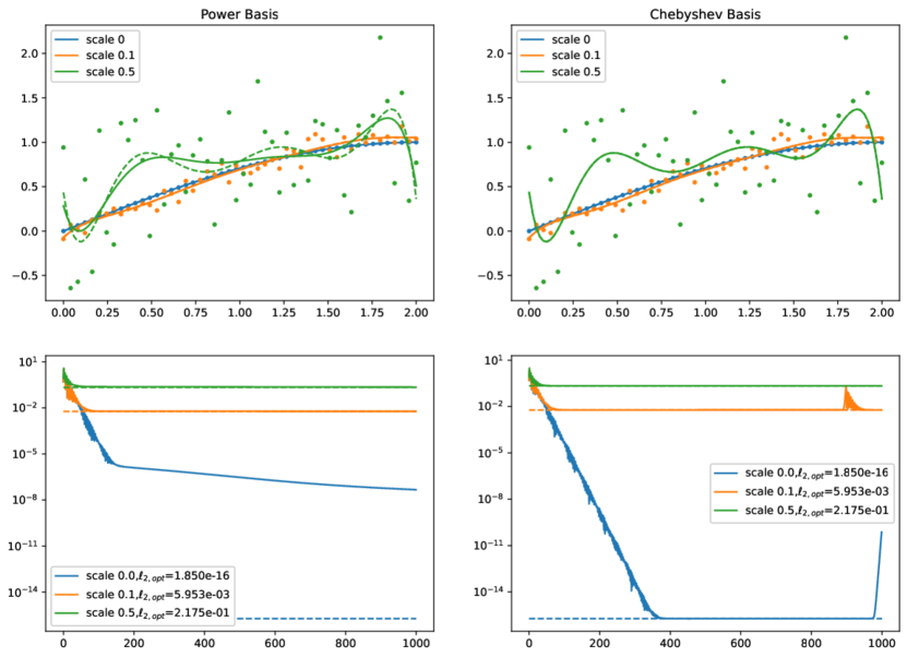
Figure 1: Results for different noise levels, AMSGrad optimizer, learning rate $1.0$, dataset A, $1$ segment, $1000$ epochs, $\alpha=0$. Top: Derivative $0$ curve shapes. Bottom: $\ell_{2}$ losses. Optima at dashed lines.

Looking at the performance of all optimizers available with TensorFlow version $2.13.0$ shows that Chebyshev basis clearly outperforms power basis with all observed datasets and optimizers converging to the optimum within $5000$ epochs. While none of the optimizers manage to reach the $\ell_{2}$ optimum with power basis in the given $5000$ epochs, there are several optimizers achieving this with Chebyshev basis. Interestingly, with Chebyshev basis, Vanilla SGD is outperforming more “elaborate” adaptive optimizers, like AMSGrad and other Adam-based optimizers. Sorted by quickest convergence, candidate optimizers are Nadam, Adagrad, FTRL, Vanilla SGD, SGD with Nesterov momentum, Adam, Adamax, AMSGrad SGD with momentum and Adadelta. As our main goal is performing combined approximation and continuity optimization, we do not look into optimizing hyperparameters of individual optimizers in the sole approximation optimization target scenario.

3.3 Optimizing $\ell$

Contrary to the single approximation target discussed in the previous section, we see that a lower learning rate of $0.1$ is beneficial. Chebyshev basis results again converge to lower losses, however, now $2000$ epochs are required. Increasing the number of segments does not affect the highest possible learning rates.

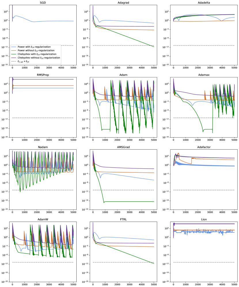
Figure 3: Losses over epochs with different optimizers with learning rate = $0.1$, $\alpha=0.1$, dataset A, $2$ segments. Dashed lines denote $\ell_{2}+\ell_{CK}$ for the respective segment-wise least squares optimum.

Looking at the performance of all optimizers available with TensorFlow version $2.13.0$, Chebyshev basis is again clearly outperforming power basis in regard to all relevant optimizers and input point sets. Fig. 3 in Appendix B shows this in more detail for dataset A: While none of the optimizers manage to surpass $\ell_{2}^{*}$ with power basis in the given $5000$ epochs, there are several optimizers achieving this with Chebyshev basis. Interestingly, however, with Chebyshev basis, SGD does not converge in this combined approximation and continuity optimization target any longer. Results with regularization of $\mathcal{C}^{k}$-loss, as introduced in Sect. 2.2, clearly outperform results without $\mathcal{C}^{k}$-loss regularization for candidate optimizers.

Running experiments with all datasets and noise levels defined in Table 1, we see the trend that more optimizers (also with power basis) manage to surpass the $\ell_{2}^{*}$ baseline for input data with higher $\ell_{2}^{*}$ values. Experiments also clearly show that results with regularization of $\mathcal{C}^{k}$-loss outperform results without $\mathcal{C}^{k}$-loss regularization for candidate optimizers also for datasets other than dataset A. The higher $\ell_{2}^{*}$ of the input data, the closer is the gap between regularized and non-regularized losses, as well as power basis and Chebyshev basis results. Considering all observed input data, AMSGrad with default parameters is the best candidate for both polynomial bases in this combined approximation and continuity optimization target. Since spikes in its total loss curve frequently occur after the optimizer has reached lowest remaining losses, however, early stopping with reverting to the best PP coefficients achieved for the training run is strongly recommended. Investigating different methods of initializing polynomial coefficients ($\ell_{2}$ optimum, zero, random), $\ell_{2}$ optimum initialization turns out to be the best choice.

A simple approach for $\mathcal{C}^{k}$-continuous solutions would be to apply Algorithm 1 to the segment-wise $\ell_{2}$ optimum. However, looking at $\ell_{2}$ versus $\ell_{CK}$ error for different datasets, as depicted in Fig. 2 for dataset A, we find that strictly establishing continuity using Algorithm 1 for a result with $\alpha=0$ increases the remaining approximation error significantly. Strictly establishing continuity for an optimization result with $\alpha>0$, on the other hand, affects prior approximation errors only mildly. This is an important finding, as it not only substantiates the need for $\ell_{CK}$ optimization, but also tells us that if we strictly establish continuity after optimization, it is beneficial to choose an $\alpha$ value that is greater but close to $0$.

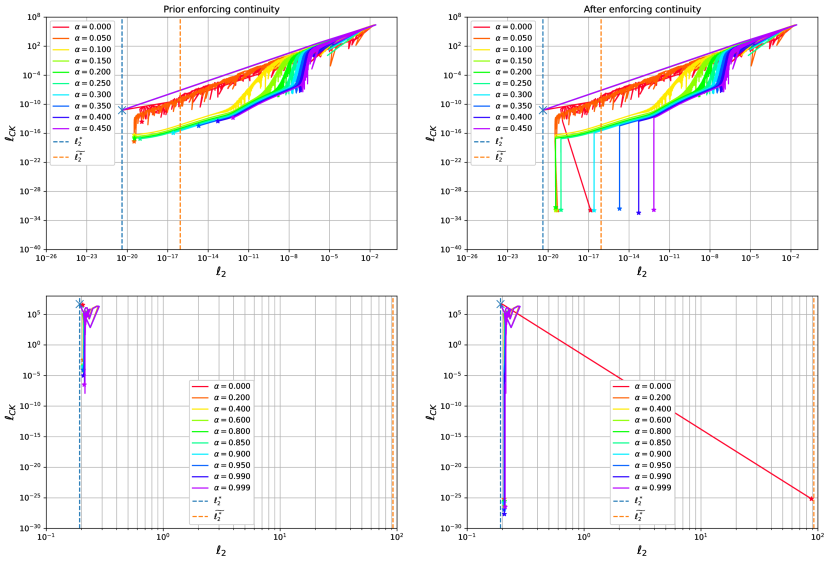
Figure 2: Continuity over approximation error for $\ell_{2}$ initialization with learning rate = $0.1$, $\alpha=0.1$, dataset A, $2$ segments, $2000$ epochs and early stopping enabled with a patience of $500$. Top: Noise scale = $0$. Bottom: Noise scale = $0.5$.

Looking at the experimental setup of Fig. 2, the margin between remaining approximation error $\ell_{2}^{*}$ of a conventional segment-wise least squares fit and approximation error $\widetilde{\ell_{2}^{*}}$ of this fit after strictly establishing continuity via algorithm is higher for input data with higher variance. Taking this margin as a baseline, higher variance input data leaves us with with a wider band of where our optimization leads to better results than performing a conventional segment-wise least squares fit with strict continuity establishment. In case of a wider band, we can also have a wider range of $\alpha$ values that make sense. Leaving out some scenarios where local optima of higher $\alpha$ values have a lower approximation error than lower ones, we generally see a tendency of rising approximation errors with rising $\alpha$ values. Considering the experimental setup of Fig. 2, the two bottom plots show results for input dataset A with a noise scale of $0.5$. Here, we observe results that lie within the aforementioned margin throughout the complete $\alpha$ range $0\leq\alpha\leq 1$. Without noise, as shown in the two top plots, the $\ell_{2}^{*}$ value of the input data is lower, and we see $\alpha$ values of $>\approx 0.3$ tendentially having ever higher approximation errors, thus leaving the margin, which leaves us with a smaller range of possible values of $\alpha$ that make sense.

4 Conclusion and Outlook

Our results show that optimization of PPs utlizing Chebyshev basis clearly outperforms power basis with tested data sets and various noise levels. Increasing the number of polynomial segments can further boost this advantage, as Chebyshev basis benefits from input data with lower variance. Considering its better performance with degree $7$ polynomials, this also makes Chebyshev basis the favorable candidate for the generation of $\mathcal{C}^{3}$-continuos PP position profiles for the use in electronic cam approximation, as a polynomial degree of $7$ is required to strictly establish $\mathcal{C}^{3}$-continuity after optimization using Algorithm 1. Looking at Chebyshev basis convergence results for different data sets, we see that the regularization method introduced in Sect. 2.2 is required to reduce oscillating behavior and boost optimizer performance.

As outlined in section Sect. 2.4, setting $\alpha>0$ leaves us with a non-convex optimization problem prone of getting stuck in unfavorable local optima. Experimental results documented in Sect. 3 show, however, that we can effectively guard against this by (i) pre-initializing polynomial coefficients with the segment-wise $\ell_{2}$ optimum, (ii) applying early stopping and reverting to best PP coefficients achieved during the training run and (iii) strictly establishing continuity after optimization with $\alpha>0$ running the algorithm introduced in Sect. 2.3. Our results show that strictly establishing continuity for a result with $\alpha=0$ increases the remaining approximation error significantly, while a result with $\alpha>0$ is only affected mildly. This substantiates the need for $\ell_{CK}$ optimization also when strictly establishing continuity after optimization.

Looking at possible future work, additional terms in $\ell$ can accommodate for further domain-specific goals. For instance, we can reduce oscillations in $f$ by penalizing the strain energy $\ell_{\text{strain}}=\int_{I}f^{\prime\prime}(x)^{2}\;\mathrm{d}{x}\,$, which, in the context of electronic cams, can reduce induced forces and energy consumption. While our approach benefits from optimizers provided with modern ML frameworks, it also has the potential of contributing back to the field of ANNs. In their preprint [5], Daws and Webster initialize Neural Networks via polynomial approximation using Legendre basis and show that subsequent training results benefit from such an initialization. Our approach could be used for such an initialization. Also, our approach is compatible to other iterative ML methods. In this way, we can utilize it for Reinforcement Learning (RL) methods based on policy gradients, like Trust Region Policy Optimization or Proximal Policy Optimization, and model the policy landscape using multivariate polynomials in an effort of improving sample efficiency of modern RL algorithms.

Appendix A Strictly Establishing Continuity

Algorithm 1 CKMIN: Strictly Establish $\mathcal{C}^{k}$-Continuity

Input: $PP,k$ $\triangleright$ Piecewise polynomial, continuity class

1:procedure CKMIN()

2:     $(p_{1},\dots,p_{m})\leftarrow PP$ $\triangleright$ $m$ polynomial pieces

3:     for $i\leftarrow 1$ to $m$ do $\triangleright$ Correct all $p_{i}$ over $[\xi_{i-1},\xi_{i}]$

4:         $A^{L}\leftarrow\left(\frac{j!}{(l-j)!}\xi_{i-1}^{l-j}\right)_{j,l=0,j}^{k,2k+1}$ $\triangleright$ Left conditions at $\xi_{i-1}$

5:         $A^{R}\leftarrow\left(\frac{j!}{(l-j)!}\xi_{i}^{l-j}\right)_{j,l=0,j}^{k,2k+1}$ $\triangleright$ Right conditions at $\xi_{i}$

6:         $b^{L}\leftarrow\left(\begin{cases}0&\text{if }i=0\\ p^{(j)}_{i-1}(\xi_{i-1})-p^{(j)}_{i}(\xi_{i-1})&\text{otherwise}\end{cases}\right)_{j=0}^{k}$ $\triangleright$ Match $p_{i-1}$

7:         $b^{R}\leftarrow\left(\begin{cases}0&\text{if }i=m\\ \frac{p^{(j)}_{i+1}(\xi_{i})-p^{(j)}_{i}(\xi_{i})}{2}&\text{otherwise}\par\end{cases}\right)_{j=0}^{k}$ $\triangleright$ Match mean of $p_{i},p_{i+1}$

8:         $A,b\leftarrow\begin{pmatrix}A^{L}\\ A^{R}\end{pmatrix},\begin{pmatrix}b^{L}\\ b^{R}\end{pmatrix}$ $\triangleright$ Stacking equation systems

9:         $c\leftarrow A^{-1}\cdot b$ $\triangleright$ Solve $A\cdot c=b$ for $c$

10:         $q_{i}\leftarrow\sum_{j=0}^{2k+1}c_{j}x^{j}$ $\triangleright$ Corrective polynomial

11:         $p_{i}\leftarrow p_{i}+q_{i}$ $\triangleright$ Apply correction

12:     end for

13:     return $(p_{1},\dots,p_{m})$ $\triangleright$ $\mathcal{C}^{k}$-continuous piecewise polynomial

14:end procedure

Appendix B Optimizer Performance

References

- [1] Adcock, B., Dexter, N.: The Gap between Theory and Practice in Function Approximation with Deep Neural Networks. SIAM Journal on Mathematics of Data Science 3(2), 624–655 (2021). https://doi.org/10.1137/20M131309X
- [2] Bostan, A., Salvy, B., Schost, E.: Fast conversion algorithms for orthogonal polynomials. Linear Algebra and its Applications 432(1), 249–258 (2010). https://doi.org/https://doi.org/10.1016/j.laa.2009.08.002
- [3] Chen, Z., Xiao, Y., Cao, J.: Approximation by piecewise polynomials on Voronoi tessellation. Graphical Models 76(5), 522–531 (2014). https://doi.org/https://doi.org/10.1016/j.gmod.2014.04.006, https://www.sciencedirect.com/science/article/pii/S1524070314000320, Geometric Modeling and Processing 2014
- [4] Datta, K., Mohan, B.: Orthogonal Functions In Systems And Control. Advanced Series In Electrical And Computer Engineering, World Scientific Publishing Company (1995)
- [5] Daws, J., Webster, C.G.: A Polynomial-Based Approach for Architectural Design and Learning with Deep Neural Networks (2019). https://doi.org/https://doi.org/10.48550/arXiv.1905.10457
- [6] Huber, S., Waclawek, H.: -continuous Spline Approximtion with TensorFlow Gradient Descent Optimizers. In: EUROCAST 2022. pp. 577–584. Springer Nature Switzerland, Cham (2023)
- [7] Josephs, H., Huston, R.: Dynamics of Mechanical Systems. CRC Press, USA, 1 edn. (2002)
- [8] Mason, J., Handscomb, D.: Chebyshev Polynomials. CRC Press (2002)
- [9] Mermelstein, S., Acar, M.: Optimising cam motion using piecewise polynomials. Engineering With Computers 19, 241–254 (02 2004). https://doi.org/10.1007/s00366-003-0264-0
- [10] Nguyen, T., Kurtenbach, S., Hüsing, M., Corves, B.: A general framework for motion design of the follower in cam mechanisms by using non-uniform rational B-spline. Mechanism and Machine Theory 137, 374–385 (2019). https://doi.org/https://doi.org/10.1016/j.mechmachtheory.2019.03.029, https://www.sciencedirect.com/science/article/pii/S0094114X18321852
- [11] Shen, Z., Yang, H., Zhang, S.: Deep Network Approximation Characterized by Number of Neurons. Communications in Computational Physics 28(5), 1768–1811 (2020). https://doi.org/https://doi.org/10.4208/cicp.OA-2020-0149, http://global-sci.org/intro/article_detail/cicp/18396.html
- [12] Waclawek, H., Huber, S.: Experimental results for publication “Machine Learning Optimized Orthogonal Basis Piecewise Polynomial Approximation”. https://github.com/hawaclawek/ml-optimized-orthogonal-basis-pp (2024), accessed: 2024-02-15